Constrain the GRB jet opening angle based on the very steep decay phase
Abstract
Thanks to the rapid follow-up observations by Swift/XRT, a good part of Gamma-Ray Bursts (GRBs) high latitude emission have been observed in X-ray band. Some of them even show a dropdown decay after this period, which strongly indicates the edge of the jet is corresponding to the breaking time. This study constrains the jet opening angles of GRBs by analyzing the very steep decay phase in the early X-ray afterglow. Using data from Swift/XRT, we identified GRBs with significant breaks in their light curves and applied a broken power-law model to describe the decay phases. Assuming a spherical and isotropic emitting surface, we set constraints on the radiation radius () to estimate jet opening angles () from the breaking time. Our results indicate that jet opening angles can be constrained, although they are sensitive to the assumed radiation radius. This approach provides yet another method for estimating GRB jet opening angles.
1 Introduction
Gamma-ray bursts (GRBs) are among the most energetic explosions in the universe, releasing tremendous amounts of energy across the entire electromagnetic spectrum over a brief period of time. These intense bursts of gamma rays are believed to originate from the collapsed remnants of massive stars (long GRBs) or the merging of compact object binaries such as neutron stars or black holes (short GRBs; see Piran 2004; Kumar & Zhang 2015 for reviews).
A key characteristic of GRBs is the existence of narrowly collimated relativistic jets produced during the explosion (Rhoads, 1999; Sari et al., 1999). The ultra-relativistic nature of these jets, with Lorentz factors typically in the range of 100-1000, is required to overcome the “compactness problem” and allow the emission of gamma rays (Lithwick & Sari, 2001). The jet’s high bulk Lorentz factor () also helps explain the non-thermal spectra observed in GRBs via particle acceleration in internal shocks within the jet (Rees & Meszaros, 1994; Daigne & Mochkovitch, 1998). In addition to the Lorentz factor, the opening angle () of the GRB jet plays a crucial role in understanding the true energetics and event rates of these phenomena (Frail et al., 2001; Bloom et al., 2003).
One of the primary methods to constrain the jet opening angle is through the observation of a “jet break” in the afterglow light curve. This jet break occurs when the relativistic beaming angle () becomes comparable to the jet opening angle (), causing a steepening in the light curve (Rhoads, 1999; Sari et al., 1999). Observations of such jet breaks in the afterglows of GRBs have provided estimates of , leading to important insights into the true energy scale of GRBs (Frail et al., 2001; Bloom et al., 2003).
The high latitude emission may emerge once the emitting shell ceases in the prompt phase. It has been observed as a steep decay phase in the early stage of the X-ray emission (Zhang et al., 2006). This happens when the photons emit from the high latitude with angle . With later time, the emitting region comes from higher latitude . Once it reaches the edge of the jet (), there should be an abrupt drop in the light curve as no more emission from even larger . We call it the dropdown decay phase. There are quite a few GRBs show such property with the decaying index down to -10.
In this work, we concentrate on this scenario. Because of the rapid response of XRT on board Swift satellite (Gehrels et al., 2004), the high latitude emission can be seen on many GRBs with XRT observations (Zhang et al., 2006). Some of them show the dropdown decay after the steep decay. This break indicates the edge of the jet, and the opening angle can be inferred in principle. We introduce the details of the model in Section 2, the data and results are given in Section 3, and the conclusions and discussions are given in section 4.
2 Model
Based on the internal shock model of the GRB emission, the prompt -rays are emitted from the shocked shells. However, the higher latitude emission may also reach to the observer at later times, and the frequency of the emission is lower as Doppler transformation effect. This shows as a steep decaying phase in the early X-ray afterglow (Zhang et al., 2006). The decay rate obeys the so-called curvature effect relation , where is the spectral index, i.e., (Kumar & Panaitescu, 2000). Considering the opening angle of the jet, once after the time the emission comes from the edge of the jet, there is no more emission can be seen from an even higher latitude. The emission drops abruptly. Other emission such as the cooling tail of the emitting region may take over the decay, and we see a dropdown () decay in the light curve. Once we find the breaking time , the opening angle of the jet can generally be determined.
The scenario is based on the following assumption. First, we assume that the emitting surface at radius is spherical and that the emission is isotropic in the comoving frame. Secondly, the jet is assumed to pointing to the observer, which is . This is roughly true, otherwise, the prompt emission of the GRBs may not be seen. Thirdly, other origins of the emission, such as the Electron-positron pair-enriched ejecta, reverse shock emission, and the energy injection (Barniol Duran & Kumar, 2009) are not considered. Otherwise, there may not exist a dropdown phase. That means, this method is not suitable for those GRBs for constraining the opening angle. We will just omit those GRBs in this work.
The breaking time from steep decay to dropdown decay is related to the jet opening angle as follows (see Hascoët et al., 2012, for example),
| (1) |
The breaking time can solely determine the combination . If we want to get the opening angle, should be determined first. However, the most commonly used relation , where is the Lorentz factor of the internal shocked jet, and is the timescale of the prompt light curve, is model dependent and parameter dependent. Here, we use the upper limit and the lower limit of to make constraints on the opening angle .
We set the lower limit based on the compactness problem, which is that the high-energy photons should be absorbed by the lower energetic photons if the radius is too small. Though, it is often used to constrain the lower limit of the Lorentz factor of GRB jet (Fenimore et al., 1993).
The other constraint on the lower limit is that the ray photons cannot escape if the optical depth is greater than 1. This induces the radius should be greater than (see equation (27) in Piran, 1999).
| (2) |
where is the isotropic equivalent kinetic energy of the GRB. is used in the whole paper. All quantities are in cgs units. Based on both constraints, we choose cm as the lower limit of the radiation radius.
For the upper limit, we set it being the deceleration radius . If is larger than , most energy should have been released through the deceleration by the circum-burst medium, and the radiation is afterglow-like, i.e., the light curve is smoother compared with the very variable prompt emission. The deceleration radius for uniform circum-burst density is (see equatoin (7.79) in Zhang, 2018)
| (3) |
where is the isotropic equivalent kinetic energy of the GRB, and is the number density of the circum-burst medium. Considering the typical is in order of ergs for a whole GRB, ergs is a proper typical isotropic equivalent kinetic energy of a certain shell. The initial Lorentz factor is a typical value. And the number density is also a typical value. Here, we set cm as a typical upper limit of . Notice for individual GRB, the upper limit could vary (not much) depending on the energy, the circum-burst density etc.
Once the is obtained, one can get the lower and upper limits of based on the upper and lower limits of given above.
3 Sample and Results
The data are selected from the light curves of Swift/XRT 111https://www.swift.ac.uk/xrt_curves/allcurves.php, with GRBs starting from GRB 041223 until GRB 231230A. In total, there are, 1422 GRBs. We visually inspected the light curves of each GRB and selected those bursts with noticeable break in the early afterglow as our preliminary data samples, as the light curve with no break can be clearly ruled out. Then we fit the light curves and classified them into golden sample, silver sample and those not included based on the criteria described later on in this section.
The behavior patterns before and after the jet break222Notice this jet break is different from the commonly called jet break during the late afterglow stage, though they are both breaks caused by jet. can be described using a broken power-law function:
| (4) |
where is a normalization term, and represent the decay indices before and after the jet break, and is the breaking time. For each GRB, the starting time () and ending time () of the two decaying stages before and after the jet break are determined through visual inspection. Then, data within this period are selected for fitting. The jet break time can be determined through the fitting. Given the time range [, ], the spectral index () before the jet break can be obtained by using the data supplied by the UK Swift Science Data Centre at the University of Leicester (Evans et al., 2009). Once the closure relation is satisfied, we confirm the decay is the high latitude emission and the fitted is the jet break time. Then can be determined through Equation (1). As discussed above in Equations (2) and (3), we choose cm and cm as the lower and upper bounds of . Consequently, the lower and upper limits for the jet opening angle are obtained through Equation (1).
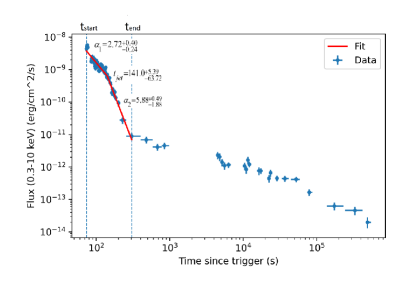
We take GRB 100425A as an example, which is shown in Figure 1. Data within the time of 70-400 s are selected for fitting. and respectively represent the times corresponding to the first and last data points within the selected time window. For GRB 100425A, = 73.7 s, = 304.4 s. Monte Carlo Markov Chain (MCMC) is employed for parameter estimation. The prior distributions of the parameters are as follows: The decay index follows a uniform distribution between 0 and 5, follows a uniform distribution between 3 and 10, the jet break time has a flat prior within the selected time window. For each GRB, the number of walkers is set to 100, and the MCMC chain length is 2000. The fitting results for GRB 100425A are , , s, which align with our expectations. Then, we can calculate using Equation (1) and constrain the jet opening angle. The calculation results for GRB 100425A show that its minimum jet opening angle , its maximum jet opening angle . is the spectral index for the time interval same as for . The values of are taken from the Swift/XRT website, by imputing the time interval (73.7 s to 141.0 s) for time-sliced spectrum (Evans et al., 2009) 333https://www.swift.ac.uk/xrt_curves/allcurves.php. We get . If , we can say the emission at this time interval is the high latitude emission tail of the prompt ray emission. However, for GRB 100425A, make the phase not likely from high latitude emission. The jet angle constraint on this GRB is doubtful.
The results for golden sample and silver sample are listed in Tables 1 and 2, respectively. The golden sample includes the GRBs with a clear break and a followed steep decay. The silver sample includes the GRBs with either a smoother break or the steep decay phase, just contains a few observing data. Both of them should satisfy the closure relation, i.e., . Otherwise, the ‘normal’ steep decay maybe does not come from the high latitude emission. Consequently, the follow-up decay maybe does not come from the jet break neither. To tolerate the possible errors, we select the GRBs with .
For those GRBs outside this region, we also list them in Tables 3 and 4, respectively. The violation of the closure relation might be that there is evolution of the spectrum, or the jet structure is not spherical. The break may still be caused by the jet edge. However, these constraints are not robustly reliable then.
It is worth checking whether the break is from the changing of the spectral index , which is measured during the period . In this case, after the break, the light curve still obeys the closure relation, i.e., . This is very unlikely for the golden samples as the breaking index is quite large, which means should be very large. For example, GRB 050814, with , is the smallest in the golden sample. for earlier WT mode photons, and for later PC mode photons. However, is similar to . It does not satisfy . This could happen for the silver samples, as is not so large for some of them. GRBs 120219A and 171209A are the two examples, with being around 1.14 and 1.46 respectively. For 120219A, for earlier WT mode photons, and for later PC mode photons, while . They marginally follow the . For GRB 171209A, there are only WT photons at this stage. , while . It is neither a confidentially high-latitude emission at a changed spectral segment. Therefore, though there are no decisive examples in the chosen data, one may be cautioned for those bursts with the even steeper decay not so steep. Checking the closure relation should be necessary before stating that the break is a jet break. We list all the values of in all 4 tables. For GRBs with both WT and PC data, we only include of the WT data, as they are always closer to the break time and should be used to investigate the spectral crossing effect.
In addition to GRBs with not enough data, we do not include GRBs with the following features: 1. The dropdown decay index is not steep enough () (e.g., GRB 080721) because the decay itself might be caused by high-latitude emission. 2. The phase does not follow a single power law decay (e.g., GRB 060202) because it is very likely not from high latitude emission. 3. The steep decay is followed by a clear flare or flares clearly dominate the whole X-ray emissions (e.g., GRB 121031A) because the jet break might be covered by the flares, even if it exists. 4. The dropdown decay exists, while the high latitude emission is missing (e.g., GRB 060428B). In this case, upper limit can be obtained as the jet break time should be smaller than the .
In table 3, for fitting the spectral index of GRB 210725A, two data modes (WT mode and PC mode) are contained in that time interval. and , and the corresponding observed flux are around and , for WT mode data and PC mode data, respectively. As the WT mode data slightly dominate the whole time interval, we choose the spectral index of the WT mode. For all other selected GRBs, there is no such issue, as the data are either only in WT mode or are clearly dominating by WT mode.
From Tables 1 and 2, one can see the combination of radius and jet opening angle is quite concentrating at cm. The distribution is cm for the golden sample, where the error is the standard deviation, cm for the silver sample, and cm for both of them. Considering Eq. (1), is actually directly related to . Therefore, the distribution of is tightly concentrated. However, this concentration is likely because of the selection effect. For shorter or longer , the break is likely covered by the X-ray flares or afterglow emissions.
Notice, in the whole work, we did not consider the redshift of each GRB. The reason is that only very few of them have redshift observations. Only 3 out of 12 GRBs in the whole golden and silver samples, while these 3 GRBs all have only photometric redshifts. Those are (photometric) for GRB 050814 (Curran et al., 2008), (photometric) for GRB 081230 (Krühler et al., 2011), and (photometric) for GRB 090404 (Perley & Perley, 2013). If the redshift is considered for these 4 GRBs, the concentration of is looser, which makes the tight distribution being intrinsic less likely.
As there are no robust methods to constrain the radius , the range of is loosely constrained, consequently. It can be seen in the last two columns of the tables.
| GRB | (s) | (s) | (s) | (cm) | ||||||
|---|---|---|---|---|---|---|---|---|---|---|
| 050814 | 166.6 | 841.4 | 0.011 | 0.464 | ||||||
| 081230 | 131.3 | 262.1 | 0.009 | 0.289 | ||||||
| 090404 | 92.0 | 196.7 | 0.008 | 0.272 | ||||||
| 150428B | 102.0 | 539.0 | 0.010 | 0.317 | ||||||
| 210818A | 53.3 | 146.9 | 0.008 | 0.269 | ||||||
| 230420A | 81.0 | 300.6 | 0.007 | 0.313 | ||||||
| 231129A | 102.1 | 281.2 | 0.009 | 0.293 |
| GRB | (s) | (s) | (s) | (cm) | ||||||
|---|---|---|---|---|---|---|---|---|---|---|
| 080503 | 82.1 | 707.6 | 0.011 | 0.371 | ||||||
| 080613B | 77.4 | 258.2 | 0.010 | 0.332 | ||||||
| 120219A | 119.3 | 582.9 | 0.009 | 0.379 | ||||||
| 160313A | 158.9 | 571.7 | 0.012 | 0.430 | ||||||
| 171209A | 93.9 | 452.9 | 0.012 | 0.381 |
| GRB | (s) | (s) | (s) | (cm) | ||||||
|---|---|---|---|---|---|---|---|---|---|---|
| 050724 | 80.3 | 471.5 | 0.011 | 0.396 | ||||||
| 060502A | 86.6 | 206.9 | 0.008 | 0.327 | ||||||
| 081221 | 73.3 | 298.7 | 0.008 | 0.257 | ||||||
| 100425A | 73.7 | 304.4 | 0.007 | 0.296 | ||||||
| 101030A | 72.9 | 224.2 | 0.008 | 0.248 | ||||||
| 101219B | 138.7 | 589.3 | 0.015 | 0.501 | ||||||
| 111123A | 94.3 | 787.5 | 0.015 | 0.501 | ||||||
| 120213A | 45.1 | 395.6 | 0.009 | 0.280 | ||||||
| 120308A | 120.6 | 299.7 | 0.011 | 0.367 | ||||||
| 151228B | 41.4 | 269.3 | 0.009 | 0.292 | ||||||
| 160501A | 120.1 | 1110.4 | 0.010 | 0.405 | ||||||
| 160804A | 138.4 | 895.2 | 0.018 | 0.560 | ||||||
| 170127A | 90.0 | 375.0 | 0.012 | 0.392 | ||||||
| 180314A | 150.9 | 382.9 | 0.012 | 0.438 | ||||||
| 180925A | 101.4 | 381.6 | 0.011 | 0.354 | ||||||
| 190219A | 91.6 | 320.7 | 0.009 | 0.292 | ||||||
| 200219A | 58.9 | 230.4 | 0.010 | 0.321 | ||||||
| 210421A | 82.7 | 404.5 | 0.007 | 0.323 | ||||||
| 210725A | 118.0 | 643.7 | 0.015 | 0.506 |
| GRB | (s) | (s) | (s) | (cm) | ||||||
|---|---|---|---|---|---|---|---|---|---|---|
| 071227 | 108.8 | 464.1 | 0.010 | 0.338 | ||||||
| 080123 | 110.4 | 549.0 | 0.011 | 0.362 | ||||||
| 100725A | 84.1 | 345.3 | 0.011 | 0.359 | ||||||
| 120326A | 52.9 | 232.0 | 0.007 | 0.259 | ||||||
| 160412A | 69.1 | 255.1 | 0.008 | 0.262 | ||||||
| 171007A | 76.7 | 374.4 | 0.010 | 0.327 | ||||||
| 181203A | 66.6 | 147.0 | 0.007 | 0.237 | ||||||
| 210912A | 49.7 | 109.4 | 0.006 | 0.212 |
4 Conclusion and discussion
In this work, we investigated the jet opening angles of Gamma-Ray Bursts (GRBs) by analyzing the steep decay phase and the dropdown decay phase observed in the early X-ray afterglow, which is attributed to high latitude emission and the edge of the jet, respectively. Using data from the Swift/XRT, we identified GRBs exhibiting a noticeable break in their light curves and employed a broken power-law model to characterize the decay before and after the break.
Our analysis is based on the assumption that the emitting surface is spherical and isotropic in the comoving frame, and that the jet is oriented towards the observer. We constrained the radiation radius using both lower and upper limits based on the compactness problem and deceleration radius, respectively. The jet opening angle was then inferred from the breaking time, which marks the transition from steep to dropdown decay.
We applied this method to GRBs with steep decays, and used a Monte Carlo Markov Chain (MCMC) for parameter estimation. The results demonstrated that the jet opening angles could be constrained within a certain range, although the exact values are dependent on the assumed radiation radius. Once there are reliable ways to constrain the radiation radius, the jet opening angle can be well determined. One should be cautioned that the even steeper decay phase () being caused by spectral crossing. In this case, the closure relation still obeys, and the break cannot be used to constrain the jet opening angle.
It is worth constraining and jointly with multi-method. Once the is determined, one may use it to determine the radius . Notice that the timescale of each GRB is easy to obtain, though the uncertainty is high and the diversity of each pulse high. However, since there are different methods to determine (see Zou et al., 2011, and references therein), and different methods might be used for different GRBs, it is difficult to find a unified method to constrain all GRBs. Therefore, one may look into the details of each burst and try to find a proper method to constrain both the and .
Acknowledgements
We thank the anonymous referee for the insightful suggestions and comments. Y.-C. Z. thanks Rodolfo Barniol Duran for the valuable discussion. This work was supported by the National SKA Program of China (2022SKA0130100). The computation was completed on the HPC Platform of Huazhong University of Science and Technology.
References
- Barniol Duran & Kumar (2009) Barniol Duran, R., & Kumar, P. 2009, MNRAS, 395, 955, doi: 10.1111/j.1365-2966.2009.14584.x
- Bloom et al. (2003) Bloom, J. S., Frail, D. A., & Kulkarni, S. R. 2003, ApJ, 594, 674, doi: 10.1086/376961
- Curran et al. (2008) Curran, P. A., Wijers, R. A. M. J., Heemskerk, M. H. M., et al. 2008, A&A, 490, 1047, doi: 10.1051/0004-6361:200810545
- Daigne & Mochkovitch (1998) Daigne, F., & Mochkovitch, R. 1998, MNRAS, 296, 275, doi: 10.1046/j.1365-8711.1998.01305.x
- Evans et al. (2009) Evans, P. A., Beardmore, A. P., Page, K. L., et al. 2009, MNRAS, 397, 1177, doi: 10.1111/j.1365-2966.2009.14913.x
- Fenimore et al. (1993) Fenimore, E. E., Epstein, R. I., & Ho, C. 1993, A&AS, 97, 59
- Frail et al. (2001) Frail, D. A., Kulkarni, S. R., Sari, R., et al. 2001, ApJ, 562, L55, doi: 10.1086/338119
- Gehrels et al. (2004) Gehrels, N., Chincarini, G., Giommi, P., et al. 2004, ApJ, 611, 1005, doi: 10.1086/422091
- Hascoët et al. (2012) Hascoët, R., Daigne, F., & Mochkovitch, R. 2012, A&A, 542, L29, doi: 10.1051/0004-6361/201219339
- Krühler et al. (2011) Krühler, T., Schady, P., Greiner, J., et al. 2011, A&A, 526, A153, doi: 10.1051/0004-6361/201015327
- Kumar & Panaitescu (2000) Kumar, P., & Panaitescu, A. 2000, ApJ, 541, L51, doi: 10.1086/312905
- Kumar & Zhang (2015) Kumar, P., & Zhang, B. 2015, Phys. Rep., 561, 1, doi: 10.1016/j.physrep.2014.09.008
- Lithwick & Sari (2001) Lithwick, Y., & Sari, R. 2001, ApJ, 555, 540, doi: 10.1086/321455
- Perley & Perley (2013) Perley, D. A., & Perley, R. A. 2013, ApJ, 778, 172, doi: 10.1088/0004-637X/778/2/172
- Piran (1999) Piran, T. 1999, Phys. Rep., 314, 575, doi: 10.1016/S0370-1573(98)00127-6
- Piran (2004) —. 2004, Reviews of Modern Physics, 76, 1143, doi: 10.1103/RevModPhys.76.1143
- Rees & Meszaros (1994) Rees, M. J., & Meszaros, P. 1994, ApJ, 430, L93, doi: 10.1086/187446
- Rhoads (1999) Rhoads, J. E. 1999, ApJ, 525, 737, doi: 10.1086/307907
- Sari et al. (1999) Sari, R., Piran, T., & Halpern, J. P. 1999, ApJ, 519, L17, doi: 10.1086/312109
- Zhang (2018) Zhang, B. 2018, The physics of gamma-ray bursts (Cambridge University Press)
- Zhang et al. (2006) Zhang, B., Fan, Y. Z., Dyks, J., et al. 2006, ApJ, 642, 354, doi: 10.1086/500723
- Zou et al. (2011) Zou, Y.-C., Fan, Y.-Z., & Piran, T. 2011, ApJ, 726, L2, doi: 10.1088/2041-8205/726/1/L2