Dynamic Localisation of Spatial-Temporal Graph Neural Network
Abstract.
Spatial-temporal data, fundamental to many intelligent applications, reveals dependencies indicating causal links between present measurements at specific locations and historical data at the same or other locations. Within this context, adaptive spatial-temporal graph neural networks (ASTGNNs) have emerged as valuable tools for modelling these dependencies, especially through a data-driven approach rather than pre-defined spatial graphs. While this approach offers higher accuracy, it presents increased computational demands. Addressing this challenge, this paper delves into the concept of localisation within ASTGNNs, introducing an innovative perspective that spatial dependencies should be dynamically evolving over time. We introduce DynAGS, a localised ASTGNN framework aimed at maximising efficiency and accuracy in distributed deployment. This framework integrates dynamic localisation, time-evolving spatial graphs, and personalised localisation, all orchestrated around the Dynamic Graph Generator, a light-weighted central module leveraging cross attention. The central module can integrate historical information in a node-independent manner to enhance the feature representation of nodes at the current moment. This improved feature representation is then used to generate a dynamic sparse graph without the need for costly data exchanges, and it supports personalised localisation. Performance assessments across two core ASTGNN architectures and nine real-world datasets from various applications reveal that DynAGS outshines current benchmarks, underscoring that the dynamic modelling of spatial dependencies can drastically improve model expressibility, flexibility, and system efficiency, especially in distributed settings.
1. Introduction
Spatial-temporal data underpins many contemporary, intelligent web applications. Often, these data exhibit spatial and temporal dependencies, indicating that the present measurement at a specific location (in either physical or abstract spaces) is causally dependent on the historical status at the same and other locations. Understanding these spatial and temporal dependencies is a crucial aspect of spatial-temporal data mining and is critical to spatial-temporal inference. Consequently, spatial-temporal graph neural networks (STGNNs) have emerged as a potent tool for modelling these dependencies, demonstrating significant success across various fields.
A subclass of STGNN, known as adaptive spatial-temporal graph neural network (ASTGNN), has brought a new perspective to the modelling of these dependencies. Unlike traditional STGNNs that use pre-defined spatial graphs containing prior knowledge, ASTGNNs adopt a data-driven approach. They start with complete graphs and learn the spatial dependency based on the data. This method allows for a more accurate and flexible representation of the spatial-temporal data. However, this approach also introduces higher computational overhead due to the usage of complete graphs.
A recent study (Duan et al., 2023b) has proposed a promising solution to this challenge through the concept of localisation. Localisation involves pruning the spatial graph to lessen the overall data exchange between nodes and the computational overhead. This reduction is feasible due to the redundancy of information provided by spatial dependency compared to temporal dependency.
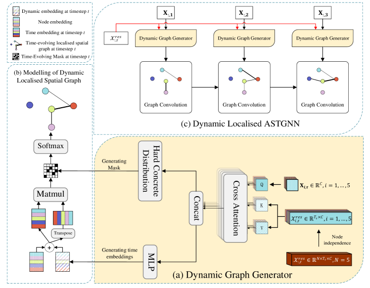
In this paper, we explore further the concept of localisation within ASTGNNs. We propose an innovative approach that transcends static spatial dependencies. We argue that the necessary spatial dependencies, modelled by the sparsified spatial graph of an ASTGNN, should not remain static across the entire time interval. Instead, these spatial dependencies, and thus the required data exchange between nodes, should be dynamically changing over time. This concept is illustrated in the section with an orange background in Figure 1: the topology and edge weights of the spatial graph are time-evolving.
Moreover, the localisation of ASTGNN is particularly useful for distributed deployments, where a reduction of data exchange between nodes can significantly enhance overall system efficiency. Existing dynamic spatial-temporal graph modeling techniques can achieve time-varying sparse graphs, but we argue this will undermine the advantages of localised ASTGNN in distributed deployment. This is because they require node-to-node data exchange at each interval to compute the spatial graph, leading to significant communication overhead, especially with large-scale and high-frequency spatial-temporal data. To this end, we proposed DynAGS, a localised ASTGNN framework designed for optimal efficiency and accuracy in distributed deployment. DynAGS has the following features:
-
•
DynAGS allows for dynamic localisation, which can further decrease the amount of data exchange by a substantial margin. Each node in our framework has the autonomy to decide whether and to which other nodes they need to send data. Importantly, this decision is made using only locally available historical data, making our framework perfectly suited for distributed deployment.
-
•
DynAGS introduces a time-evolving spatial graph, in which both the topology of the spatial graph, represented by a mask matrix, and the edge weights of the spatial graph, represented by the adjacency matrix, are dynamic. This feature guarantees optimal expressibility and flexibility of the model, and results in the minimal data exchange necessary to sustain the desired performance.
-
•
DynAGS supports personalised localisation, permitting each node to select a personalised trade-off between data traffic and inference accuracy. This flexibility allows each node to maximise its performance based on the available resources, thereby optimising the efficiency and performance of the entire heterogeneous system.
To achieve these features, the DynAGS is designed around a central module known as the Dynamic Graph Generator (DGG). Central to this module is a cross-attention mechanism. This mechanism adeptly amalgamates patch-level historical data with point-level current observational data to synthesize representations pertinent to the present time. Such representations are then utilised to generate time-evolving spatial graphs. These representations adept in the comprehensive integration of multi-scale temporal dependencies. This integration facilitates more nuanced modeling of temporal dependencies, spanning both long-term and short-term spectra, encapsulating elements such as periodicity, proximity, and trend dynamics. Consequently, this leads to an enhanced calibration of incoming weights and connections for each respective node in the system. An overview of DynAGS is illustrated in Figure 1. The main contributions of our work are as follows:
-
•
We introduce DynAGS, a novel ASTGNN framework designed for optimal efficiency and inference accuracy in distributed deployment. This framework features dynamic localisation, time-evolving spatial graphs, and personalised localisation to reduce data exchange, enhance model flexibility, and allow nodes to optimise performance based on their own available resources.
-
•
The performance of DynAGS is assessed using two backbone ASTGNN architectures across nine real-world spatial-temporal datasets. The experimental findings indicate that DynAGS significantly outperforms the state-of-the-art across various localisation degrees, ranging from 80% to 99.9%. Specifically, DynAGS, when operating at a localisation degree of 99.5%, produces results that are comparable to or even superior to those of the current leading baseline at a localisation degree of 80%. This results in a considerable decrease in communication overhead, reducing it by no less than 30 times.
-
•
The efficacy of DynAGS in diverse evaluation experiments substantiates our proposition that spatial dependency is intrinsically time-dependent. This means that the necessary spatial dependencies, and hence the required data exchange between nodes, should continually evolve over time rather than remain static. By embracing this dynamic approach in modelling spatial dependencies within ASTGNNs, we enhance the model’s expressibility and flexibility, and optimise system efficiency - a particularly significant improvement in distributed deployments.
2. Related Work
2.1. Spatial-Temporal Graph Neural Networks
STGNNs excel at uncovering hidden patterns in spatial-temporal data (Wu et al., 2020), primarily by modeling spatial dependencies among nodes through adjacency matrices. These matrices are constructed using either pre-defined or self-learned methods.
Pre-defined STGNNs use topological structures (Guo et al., 2021; Yu et al., 2018a) or specific metrics (e.g., POI similarity) to build graphs (Geng et al., 2019; Yao et al., 2018), but they rely heavily on domain knowledge and graph quality. Given the implicit and complex nature of spatial-temporal relationships, self-learned methods for graph generation have risen in prominence. These methods provide innovative approaches to capture intricate spatial-temporal dependencies, offering a significant advantage over traditional pre-defined models.
Self-learned STGNNs are divided into two primary categories: feature-based and random initialized methods. Feature-based approaches, like PDFormer (Jiang et al., 2023a) and DG (Peng et al., 2021), generate dynamic graphs from time-varying inputs, enhancing model accuracy. Random initialized STGNNs, or ASTGNNs, perform adaptive graph generation via randomly initialized learnable node embeddings. Graph WaveNet (Wu et al., 2019) propose an AGCN layer to learn a normalized adaptive adjacency matrix, and AGCRN (Bai et al., 2020) designs a Node Adaptive Parameter Learning enhanced AGCN (NAPL-AGCN) to learn node-specific patterns. Due to its notable performance, NAPL-AGCN has been integrated into various recent models (Jiang et al., 2023b; Choi et al., 2022; Chen et al., 2022). However, their static node embeddings limit the adaptability of the graphs. Recent advancements like DGCRN(Li et al., 2023) and DMSTGCN (Han et al., 2021) introduce dynamic node embeddings, allowing for more flexible graph generation in ASTGNNs. Despite these advancements, most self-learned STGNNs generate complete graphs with high computational and communication overheads. Methods such as GTS and ASTGAT mitigate this by employing strategies like Top-K and Gumbel-softmax for partial adjacency matrix retention, enabling discrete and sparse graph generation with dynamic topologies.
Yet, these approaches still require computation of all node pair connections to determine if there are edges between them, leading to a quadratic increase in data exchange and computational overhead. Our work addresses these challenges in dynamic graph generation, proposing a novel approach in localised STGNNs. By implementing dynamic localisation, we enhance model expressiveness and flexibility, while considerably reducing data exchange requirements and computational overhead. This results in a more efficient balance between model efficiency and accuracy.
2.2. Graph Sparsification for GNNs
With the increasing size of graphs, the computational cost of training and inference for GNNs also rises. This escalating cost has spurred interest in graph sparsification, which aims to create a smaller sub-graph while preserving the essential properties of the original graph (Duan et al., 2023b). SGCN (Li et al., 2020b) is the pioneering work in graph sparsification for GNNs, which involves eliminating edges from the input graph and learning an additional DNN surrogate model. More recent works, such as UGS (Chen et al., 2021b) and GBET (You et al., 2022), examine graph sparsification from the perspective of the lottery ticket hypothesis.
The aforementioned works only studied graph sparsification for standard GNNs with non-temporal data and pre-defined graphs. AGS (Duan et al., 2023b) extended this concept to spatial-temporal GNNs with adaptive graph architectures, known as the localisation of ASTGNNs. However, AGS localises an ASTGNN by learning a fixed mask, overlooking the fact that spatial dependency varies over time. This approach led to sub-optimal generalisation on unseen data. Unlike AGS, DynAGS allows the dynamic localisation of ASTGNNs.
3. PRELIMINARIES
3.1. Notations and Problem Definition
Frequently used notations are summarised in Table 1.
| Notation | Definition |
| the spatial graph used for modelling the spatial dependency | |
| the adjacency matrix of | |
| the number of nodes | |
| features of the -th node at timestep | |
| the normalised adaptive adjacency matrix | |
| dynamic adaptive adjacency matrix at timestep | |
| dynamic mask to localise ASTGNN at timestep | |
| the look-back period length of the task | |
| the dimension of node embedding | |
| the dimension of node feature | |
| the dimension of output feature of ASTGNN | |
| kernel and stride size of 1D average pooling | |
| weighting factor of -norm | |
Following the conventions in related works (Seo et al., 2018; Yu et al., 2018b; Yan et al., 2018; Bai et al., 2019; Huang et al., 2020), we denote the spatial-temporal data as a sequence of frames: , where a single frame is the -dimensional data collated from different locations at time . For a chosen task time , we aim to learn a function mapping the historical observations into the future observations in the next timesteps:
| (1) |
3.2. Localised ASTGNN
3.2.1. Graph Convolution Network
A basic method to model the spatial dependency at time is the Graph Convolutional Network (GCN) (Wu et al., 2019; Bai et al., 2019; Huang et al., 2020). A graph convolutional layer processing one data frame is defined as (Zhang et al., 2019):
| (2) |
where is the activation function, is the adjacency matrix of the graph with added self-connections (with the original adjacency matrix being ), and is the diagonal degree matrix of . is a trainable parameter matrix. is the layer output, with indicating the number of output feature dimensions for each node.
3.2.2. Adaptive Spatial-Temporal Graph Neural Network (ASTGNN)
A crucial enhancement in modeling the spatial network is the adoption of Adaptive Graph Convolution Networks (AGCNs). These networks capture the dynamics within the graph, paving the way for the development of Adaptive Spatial-Temporal Graph Neural Networks (ASTGNNs) (Wu et al., 2019; Bai et al., 2020; Chen et al., 2021a; Choi et al., 2022; Chen et al., 2022).
In the subsequent discussion, we provide a brief overview of two representative ASTGNN models: (i) The Adaptive Graph Convolutional Recurrent Network (AGCRN) (Bai et al., 2020); (ii) STG-NCDE (Choi et al., 2022), which is an extension of AGCRN with neural controlled differential equations (NCDEs).
-
•
AGCRN. AGCRN enhances the GCN layer by merging the normalised self-adaptive adjacency matrix with Node Adaptive Parameter Learning (NAPL), creating an integrated module known as NAPL-AGCN.
(3) In this context, , , and consequently . represents the normalised self-adaptive adjacency matrix (Wu et al., 2019). denotes the embedding dimension. Each row of embodies the embedding of a node. The embedding of the -th node, represented by the -th row in , is denoted as . During training, is updated to encapsulate the spatial dependencies among all nodes. Rather than learning the shared parameters in (2), NAPL-AGCN employs to learn parameters specific to each node. To capture both spatial and temporal dependencies, AGCRN combines NAPL-AGCN and Gated Recurrent Units (GRU), replacing the MLP layers in NAPL-AGCN with GRU layers.
-
•
STG-NCDE. STG-NCDE extends AGCRN by incorporating two neural controlled differential equations (NCDEs): a temporal NCDE and a spatial NCDE.
3.2.3. Localisation of ASTGNN
We denote an ASTGNN model as , where encompasses all the learnable parameters, and represents the spatial graph. The graph is characterised by its adjacency matrix , as derived from (3). The localisation of is accomplished by pruning the spatial graph . This can be mathematically expressed as the Hadamard product of the adjacency matrix and a mask matrix . Consequently, the pruned graph has the adjacency matrix . During the pruning process, is obtained by minimising the following objective:
| (4) |
Here, is the training loss function calculated with the pruned spatial graph, is the -norm, and the weighting factor regulates the degree of pruning. As is not differentiable, Adaptive Graph Sparsification (AGS) (Duan et al., 2023b), a recent localisation framework for ASTGNNs, resolves this issue by optimising the differentiable approximation of the -regularisation of .
However, in this paper, we contend that a static mask and a static adjacency matrix disregard the fact that spatial dependencies are dynamic over time, resulting in sub-optimal performance on unseen data. Consequently, we aim to achieve dynamic localisation by learning dynamic and , which are adapted to the timestep .
4. Method
To enable dynamic localisation, it is necessary to generate the time-evolving mask matrix and adaptive adjacency matrix as mentioned in Sec. 3.2. To achieve this, we have designed a framework, DynAGS, built around a core module known as the Dynamic Graph Generator (DGG). An overview of the DynAGS framework is provided in Figure 1.
4.1. Dynamic Graph Generator (DGG)
As outlined in Sec. 3.1, in most spatial-temporal tasks, the look-back period is typically much shorter than the entire time interval covered by the available data. Previous studies have predominantly utilized point-level data from the look-back period for the generation of dynamic graphs, where . This approach, however, lacks the integration of multi-scale information within the temporal dimension and falls short in modeling long-term dependencies. Accordingly, for the -th node at a chosen task time , our DGG fuses the observations in the look-back period with insights from residual historical data by a cross attention. For the -th node at a chosen task time , we define the residual historical data: .
For the -th node at timestep , a cross attention accepts the node-specific residual historical data as key and value, and the observation at the moment as the query. The cross attention then output an vector , which is subsequently utilised to determine the incoming weights and connections of the corresponding node, as detailed in Sec. 4.2. Note that in practice, we put an upper-limit on the length of based on datasets to ensure that the computational cost is acceptable. This may change the to .
4.1.1. Down-sampling and Patching
The first challenge lies in efficiently representing the residual historical data, given that the length of this data, , is extremely large. Several studies on time-series processing propose reducing the input length via down-sampling or patching. In this case, we employ a combination of both methods to significantly decrease the length of the encoder input. For the -th node, given the residual historical data , we first apply 1D average pooling with a kernel and stride over on the time dimension to down-sample it into of its original slice:
| (5) |
Next, we divide into non-overlapping patches of length to obtain a sequence of the residual historical patches , . With the use of down-sampling and patching, the number of tokens can be reduced from to .
Down-sampling and patching are applied for several reasons:
-
•
To manage residual historical data within time and memory constraints, down-sampling and patching are essential.
-
•
Down-sampling effectively retains key periodic and seasonal information from spatial-temporal data, which often includes redundant temporal details (Duan et al., 2023a).
-
•
From a temporal perspective, spatial-temporal mining seeks to understand the correlation between data at each time step. Patching captures comprehensive semantic information that is not available at the point-level by aggregating time steps into subseries-level patches (Nie et al., 2023).
4.1.2. Cross Attention
We utilise a cross-attention to process the residual historical patches and standard historical observations. These patches and observations are initially processed by two trainable linear layers, respectively. During inference, for the -th node at timestep :
| (6) |
where and , is the position embeddings. Then, we apply cross-attention operations in the temporal dimension to model the interaction between:
| (7) |
In the end, the cross-attention outputs from the nodes are stacked together to form a matrix This matrix is used later to generate the time-evolving and , which is explained in details in Sec. 4.2.
In summary, the attention mechanism within DGG selectively concentrates on sequences of historical data patches most pertinent to the current input. This process culminates in the final fused feature representation, , a thorough amalgamation of both current observation and historical data characteristics. The influence of historical data on the model’s performance is elaborated in Sec. 6.1.
4.2. Dynamic Localised ASTGNNs
Given a task time (as defined in Section 3.1), at the timestep , we need to facilitate dynamic localisation by generating of the time-evolving mask matrices and adaptive adjacency matrices .
4.2.1. Dynamic Mask Generation
The process of generating the mask matrix, , at timestep begins with a linear transformation applied to :
| (8) |
where is a trainable parameter matrix. The output of this transformation, , is then utilised to generate through hard concrete distribution sampling. Each entry is converted into binary ”gates” using the hard concrete distribution. This distribution is a continuous relaxation of a discrete distribution and can approximate binary values. The computation of the binary ”gates” is expressed as follows:
| (9) | ||||
In this equation, is randomly sampled from a uniform distribution and represents the temperature value. Following (Duan et al., 2023b), we set and in practice.
For the -th node, the corresponding can be mapped into , the -th row of . This vector determines whether the -th node needs to send data to other nodes, and this decision is solely dependent on . In other words, the -th node can independently decide whether to send data to other nodes without requiring any additional prior data exchange. The mask , which determines the topology of the spatial graph, evolves over time as it is computed from the cross attention output at time .
4.2.2. Dynamic Adaptive Graph Generation
The NAPL-AGCN employed in ASTGNN only supports a static adjacency matrix, . In order to accommodate a time-evolving , we modify the node embedding used to generate in (3) as follows:
| (10) |
Here, is the time-evolving embedding, are learnable parameters. signifies the time-evolving modification applied to the original node embedding . It’s worth noting that even though the computation is expressed in matrix forms, each row’s computation in , or , solely depends on . This implies that the computation of the node-specific time-evolving embedding, , is performed purely locally without the need for previous data exchange. This process is akin to dynamic mask generation.
To avoid calculating the entire matrix multiplication as in (3), which would necessitate all nodes to share their own time-evolving embedding with each other at every timestep, thereby causing substantial communication overhead, we propose using the locally available time-evolving mask vector . This vector already determines for the -th node which neighbours it needs to communicate with at time . Consequently, each element in the time-evolving adjacency matrix is calculated in a similar fashion to the graph attention network (GAT) (Velickovic et al., 2018):
| (11) |
Here is a set of the -th node’s neighbours in the sparse spatial graph. Even though the computation in (11) still necessitates the exchange of the time-evolving node embedding among neighboring nodes, this requirement has been significantly reduced. Moreover, the node embedding is quite small in comparison to the volume of data exchanged between adjacent nodes. Consequently, the total communication overhead necessary to support the dynamic spatial graph is minimal.
Finally, we substitute for in (3) to obtain the dynamic localised ASTGNN:
| (12) |
4.2.3. Dynamic Adaptive Graph Sparsification
Combining the time-evolving mask matrices and adjacency matrices , we define the procedure for dynamic adaptive graph sparsification as follows:
| (13) |
In this equation, represents the training loss function computed with the dynamically pruned graph, which is masked by at timestep . is the objective function that can be trained end-to-end using the Adam optimiser.
4.3. Further Enhancements
Here we discuss two additional enhancements made to our DynAGS, which improve its efficiency further.
4.3.1. Efficient Dynamic Localisation
The generation of a dynamic mask increases the time complexity to during inference. To address this, we significantly enhance the efficiency of DynAGS by initiating from a sparse spatial graph, pre-localised using AGS. Given a pre-defined graph sparsity , we first train a -localised ASTGNN or use a predefined adjacency matrix with a sparsity of (if available) to achieve efficient inference. Here, represents the graph sparsity ( means totally sparse), and is a mask matrix with a sparsity of . Based on the -localised ASTGNN, we only need to map entries into the corresponding . This reduces the time complexity to during inference, which is significant considering that is normally larger than 80%.
4.3.2. Personalised Adaptive Graph Sparsification
In real-world systems, the resources available to different nodes can vary. Consequently, we have implemented personalised localisation instead of global localisation. The node-independent processing of cross attention allows us to assign a unique weighting factor, , to adjust the degree of localisation for each node :
| (14) |
4.4. Efficiency Analysis
4.4.1. Complexity Analysis
Dynamic localization notably decreases the complexity involved in generating dynamic graphs in ASTGNNs. The inference time complexity of unpruned NAPL-AGCN layers per timestep is . After sparsification, the inference time complexity of NAPL-AGCN layers is . where denotes the number of nodes, is the number of layers, is the size of node embedding, is the size of node feature, and is the number of remaining edges. For more comparative analysis on the complexity of AGS and DynAGS, please refer to Appendix A.2.
4.4.2. Communication Analysis
This section presents a theoretical analysis of the communication costs for DynAGS and unpruned ASTGNNs. For unpruned ASTGNNs, the communication overhead during inference is:
| (15) |
In contrast, DynAGS significantly reduces this overhead:
| (16) |
We also experiment the reduction of communication costs in real-world application in Sec. 5.3.
5. Experiments
5.1. Experimental Setup
Datasets. DynAGS was evaluated on nine real-world spatial-temporal datasets from four web applications: transportation, blockchain, and biosurveillance forecasting. For a more comprehensive evaluation of the generalisation ability, particularly extrapolation to new data, it was necessary to introduce distribution shifts into the training and testing data. This goal was achieved by using more challenging settings rather than standard ones in these domains:
-
•
The training/validation/testing sets are split by time. Consequently, less data is used for both training and testing. This approach creates a larger time gap between the training set and testing set than the standard setting. This type of dataset splitting introduces a distribution shift between training and testing data, as the distributions of spatial-temporal data change over time.
-
•
We use longer input and output lengths for historical observations (inputs) to predict future observations (outputs). The spatial-temporal dependencies of inputs and outputs may differ over a large time span, as time progresses. This approach can introduce a more significant temporal shift between input and output.
Detailed information for each datasets and their configurations are provided in Appendix A.1.
Baseline. AGS(Duan et al., 2023b) was selected as the sole baseline because, to the best of our knowledge, AGS is currently the only method specifically designed for the localisation of ASTGNNs. Moreover, it represents a state-of-the-art method that was published recently. We benchmarked the performance of DynAGS against AGS using two representative ASTGNN backbone architectures: AGCRN and STG-NCDE. AGCRN stands out as the most representative ASTGNN for spatial-temporal forecasting, while STG-NCDE serves as a state-of-the-art extension of AGCRN.
Implementation. The dataset-specific hyperparameters of AGCRN and STG-NCDE, followed the same setup as in the original papers. Other dataset-specific hyperparameters for reproducibility are provided in Appendix A.3.
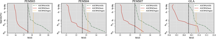
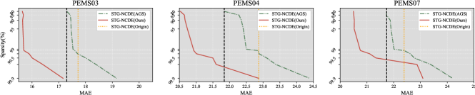
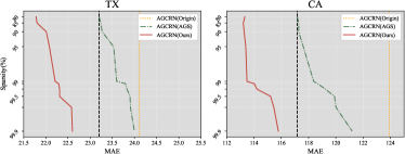
5.2. Test Accuracies
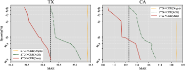
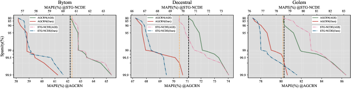
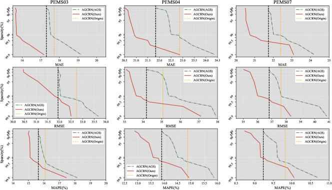
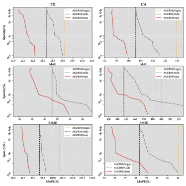
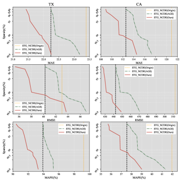
Test accuracies (MAE) of AGCRN and STG-NCDE, localized by DynAGS and AGS across localisation degrees from to , are presented in Figure 2 , Figure 3 and Figure 4 for transportation,biosurveillance and blockchain datasets, respectively. From these results, the following observations can be made:
-
•
DynAGS is adept at capturing dynamic spatial-temporal dependencies and delivers promising predictions for unseen data. Additionally, our DynAGS enhances the performance of AGS noticeably. For the same localisation degree, ours surpasses AGS by up to less error across all datasets.
-
•
DynAGS excels in the trade-off between data exchange and accuracy. When compared to AGS at a localisation degree of , DynAGS at a localisation degree of frequently attains comparable or even superior accuracies, implying that nearly 40 times less communication is needed to sustain the same performance.
-
•
The results from the GLA dataset indicate that DynAGS consistently outperforms AGS. This demonstrates that DynAGS can be scaled up to large-scale spatial-temporal data.
-
•
The accuracy of DynAGS does not always decrease as sparsity increases (e.g., Figure 6). We believe this is due to the regularization effect of sparsifying the spatial graph, which suggests that non-localized AGCRNs and STG-NCDEs suffer from overfitting to a certain degree.
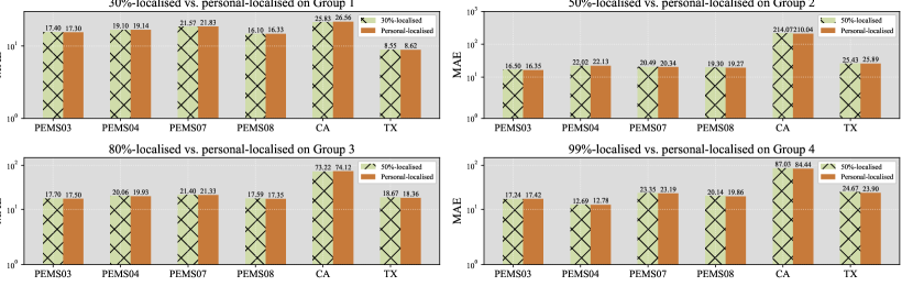
5.3. Impact on Resource Efficiency
As highlighted in Sec. 5.2, an ASTGNN localised via DynAGS to the degree of 99.5% (average degree over timesteps) delivers results comparable or even better than that with AGS to a localisation degree of 80%. Thus, we evaluated the computational demand during the inference of 99.5%-localised AGCRN and STG-NCDE via DynAGS and during the inference of 80%/99.5%-localised AGCRN and STG-NCDE via AGS. We also simulated the distributed computation of DynAGS using Python’s multiprocessing library and compared the communication cost during inference of 99.5%-localised AGCRN via DynAGS and during the inference of 80%/99.5%-localised AGCRN via AGS, as shown in Table 4. The detailed description of simulation can be found in Appendix A.6.
Our findings reveal that (i) both DynAGS and AGS can effectively reduce the computation required for inference, (ii) comparing DynAGS and AGS shows that DynAGS has a marginally higher computing cost for AGCRN but is more efficient for STG-NCDE when performance is similar, and (iii) DynAGS cuts communication cost by a factor of nearly 40 relative to AGS. Additionally, when the sparsity is the same, the computational overhead of DynAGS is still slightly higher than that of AGS, but the performance of the former is significantly better than the latter.
In real-world distributed deployment scenarios, a significant portion of resources is allocated to communication between nodes, often overshadowing local computation costs (Li et al., 2009; abd Li Rongcong, 2019). In this light, the marked reduction in communication cost by DynAGS becomes especially significant. The minor rise in local computation by DynAGS is less concerning, given that local computation is generally less resource-intensive than inter-node communication.
Thus, these outcomes affirm that the advantages of DynAGS, predominantly the substantial communication cost savings, more than compensate for the occasional minor upticks in computational demand. This positions DynAGS as a more resource-efficient solution in real-world distributed deployment contexts.
6. Ablation Studies
| Methods | Computation Cost for Inference (GFLOPs) | ||||||
| PEMS03 | PEMS04 | PEMS07 | GLA | By/De/Go | CA | TX | |
| Original AGCRN | 5.40 | 4.25 | 24.71 | 192.69 | 0.16 | 0.89 | 5.49 |
| 80%-localised AGCRN(AGS) | 2.26(2.40) | 1.93(2.20) | 5.57(4.43) | 48.18(4.00) | 0.09(1.78) | 0.81(1.11) | 3.69(1.49) |
| 99.5%-localised AGCRN(AGS) | 2.05(2.63) | 1.80(2.36) | 4.07(6.07) | 12.96(14.86) | 0.09(1.78) | 0.78(1.14) | 3.64(1.51) |
| 99.5%-localised AGCRN(Ours) | 2.63(2.05) | 2.26(1.88) | 6.51(3.80) | 13.52(14.24) | 0.12(1.39) | 0.85(1.05) | 3.88(1.41) |
| Original STG-NCDE | 21.63 | 18.55 | 53.36 | – | 3.16 | 0.47 | 2.14 |
| 80%-localised STG-NCDE(AGS) | 15.96(1.36) | 14.38(1.28) | 18.87(2.83) | – | 2.91(1.09) | 0.44(1.08) | 1.44(1.48) |
| 99.5%-localised STG-NCDE(AGS) | 14.58(1.48) | 13.37(1.39) | 10.46(5.10) | – | 2.90(1.09) | 0.44(1.08) | 1.36(1.57) |
| 99.5%-localised STG-NCDE(Ours) | 14.93(1.45) | 13.67(1.35) | 11.2(4.76) | 8.85(1.16) | 2.96(1.07) | 0.46(1.02) | 1.42(1.50) |
| Model | PEMS03 | PEMS04 | PEMS07 | ||||||
| Metric | MAE | RMSE | MAPE(%) | MAE | RMSE | MAPE(%) | MAE | RMSE | MAPE(%) |
| Z-GCNET | 18.59 | 34.08 | 18.72 | 23.15 | 36.21 | 15.97 | 26.47 | 42.13 | 11.23 |
| STG-NCDE | 17.83 | 33.72 | 17.51 | 23.44 | 35.34 | 15.21 | 25.87 | 40.41 | 10.63 |
| TAMP-S2GCNets | 17.72 | 32.74 | 16.08 | 23.40 | 36.43 | 14.88 | 22.39 | 37.63 | 9.82 |
| 99.5-localised AGCRN(via DynAGS) | 16.24 | 32.61 | 15.59 | 22.87 | 34.84 | 15.53 | 21.88 | 38.01 | 9.53 |
| Method | AGCRN | 80%-localised(AGS) | 99.5%-localised(AGS &Ours) |
| GLA | 168.22 | 33.64 | 0.91 |
| PEMS07 | 8.92 | 1.78 | 0.05 |
6.1. Impact of Residual Historical Data and Dynamic Graph
We evaluated the effects of residual historical data and dynamic graph on AGCRN (on PEMS07, Bytom, and TX datasets) by comparing DynAGS with its variants, DynAGS and DynAGS . The variant DynAGS is obtained by removing the cross attention, thereby eliminating the residual historical data. In contrast, the DynAGS variant uses only the node embedding to generate a static mask, similar to AGS, resulting in a fixed spatial graph topology over time.
As observed from Table 5, DynAGS consistently outperforms DynAGS and DynAGS by a significant margin. These results confirm that (i) the large-scale temporal features and global information provided by the residual historical data contribute positively to the performance of DynAGS, and (ii) dynamic graph modeling, which captures evolving spatial-temporal dependencies, significantly improves prediction performance.
6.2. DynAGS vs. Other Non-Localised ASTGNNs
Recent advancements in ASTGNNs have introduced improved architectures of AGCRN, including Z-GCNETs (Chen et al., 2021a), STG-NCDE (Choi et al., 2022), and TAMP-S2GCNets (Chen et al., 2022), tailored for various applications. This motivates us to evaluate how our localised AGCRNs compare to these advanced variations.Results are shown in Table 3. Our results demonstrate that the localised AGCRNs consistently achieve superior inference performance, even surpassing state-of-the-art architectures, while significantly reducing computational complexity, thereby underscoring their efficacy and practicality.
| Method | Sparsity | PEMS07 | Bytom | TX | ||
| MAE | MAPE(%) | MAPE(%) | MAE | MAPE(%) | ||
| AGCRN (DynAGS) | 50% | 21.63 | 9.22 | 62.36 | 23.24 | 96.21 |
| 80% | 21.00 | 8.91 | 61.99 | 23.20 | 96.80 | |
| 99% | 21.29 | 10.43 | 65.10 | 23.80 | 98.30 | |
| AGCRN (DynAGS ) | 50% | 23.63 | 11.03 | 65.12 | 24.50 | 98.21 |
| 80% | 22.89 | 10.57 | 65.23 | 24.37 | 98.42 | |
| 99% | 23.17 | 10.86 | 66.78 | 24.77 | 101.69 | |
| AGCRN (DynAGS ) | 50% | 24.06 | 11.41 | 66.07 | 24.99 | 100.09 |
| 80% | 23.17 | 11.27 | 67.63 | 24.24 | 99.53 | |
| 99% | 24.29 | 11.95 | 67.98 | 26.01 | 103.79 | |
6.3. Personalised Localisation
To further validate our personalised localisation approach, we conducted an additional ablation study. We divided all nodes into distinct groups, with each group assigned a specific in-degree compression ratio. Instead of merely testing these groups, we introduced a variation: while keeping a group’s in-degree compression ratio unchanged, we adjusted the ratios of the other groups. The results from this exercise were clear. The performance of a particular group remained unaffected by the in-degree sparsity alterations of other groups.
This experimental evidence underscores the fact that personalising the localisation of ASTGNNs doesn’t detract from performance, but rather presents a compelling and practical method. Further details of this experiment can be found in Appendix A.7.
7. Conclusion
This study introduced DynAGS, an innovative ASTGNN framework that dynamically models spatial-temporal dependencies. Through the integration of dynamic localisation and a time-evolving spatial graph, DynAGS has proven superior in performance across various real-world datasets, demonstrating significant reductions in communication overhead. Our findings underscore the intrinsic time-dependent nature of spatial dependencies and advocate for a shift from static to dynamic representations in spatial-temporal data analysis. Looking ahead, DynAGS paves the way for future advancements in the realm of spatial-temporal data mining, emphasising both adaptability and efficiency.
8. Acknowledgment
We thank the reviewers for their constructive comments. Wenying Duan and Shujun Guo’s research was supported in part by Jiangxi Provincial Natural Science Foundation No. 20242BAB20066. Wei Huang’s research was supported by NSFC No.62271239, and Jiangxi Double Thousand Plan No.JXSQ2023201022. Zimu Zhou’s research was supported by Chow Sang Sang Group Research Fund No. 9229139. Sincere thanks to Xiaoxi and Wenying’s mutual friend, Te sha, for providing the academic exchange platform.
References
- (1)
- abd Li Rongcong (2019) Liang Liwei abd Li Rongcong. 2019. Research on intelligent energy saving technology of 5G base station based on A. Mobile Communications 43, 12 (2019), 32–36.
- Bai et al. (2019) Lei Bai, Lina Yao, Salil S. Kanhere, Xianzhi Wang, and Quan Z. Sheng. 2019. STG2Seq: Spatial-Temporal Graph to Sequence Model for Multi-step Passenger Demand Forecasting. In Proceedings of the Twenty-Eighth International Joint Conference on Artificial Intelligence, IJCAI 2019, August 10-16, 2019, Sarit Kraus (Ed.). ijcai.org, Macao, China, 1981–1987.
- Bai et al. (2020) Lei Bai, Lina Yao, Can Li, Xianzhi Wang, and Can Wang. 2020. Adaptive graph convolutional recurrent network for traffic forecasting. In Advances in Neural Information Processing Systems. Virtual Event, 17804–17815.
- Chen et al. (2001) Chao Chen, Karl Petty, Alexander Skabardonis, Pravin Varaiya, and Zhanfeng Jia. 2001. Freeway Performance Measurement System: Mining Loop Detector Data. Transportation Research Record 1748, 1 (2001), 96–102. https://doi.org/10.3141/1748-12
- Chen et al. (2021b) Tianlong Chen, Yongduo Sui, Xuxi Chen, Aston Zhang, and Zhangyang Wang. 2021b. A Unified Lottery Ticket Hypothesis for Graph Neural Networks. In Proceedings of the 38th International Conference on Machine Learning, ICML 2021, 18-24 July 2021, Virtual Event (Proceedings of Machine Learning Research, Vol. 139), Marina Meila and Tong Zhang (Eds.). PMLR, 1695–1706.
- Chen et al. (2022) Yuzhou Chen, Ignacio Segovia-Dominguez, Baris Coskunuzer, and Yulia R. Gel. 2022. TAMP-S2GCNets: Coupling Time-Aware Multipersistence Knowledge Representation with Spatio-Supra Graph Convolutional Networks for Time-Series Forecasting. In The Tenth International Conference on Learning Representations, ICLR 2022, Virtual Event, April 25-29, 2022.
- Chen et al. (2021a) Yuzhou Chen, Ignacio Segovia-Dominguez, and Yulia R. Gel. 2021a. Z-GCNETs: Time Zigzags at Graph Convolutional Networks for Time Series Forecasting. In Proceedings of the 38th International Conference on Machine Learning, ICML 2021, 18-24 July 2021, Virtual Event (Proceedings of Machine Learning Research, Vol. 139), Marina Meila and Tong Zhang (Eds.). PMLR, 1684–1694.
- Choi et al. (2022) Jeongwhan Choi, Hwangyong Choi, Jeehyun Hwang, and Noseong Park. 2022. Graph Neural Controlled Differential Equations for Traffic Forecasting. In Thirty-Sixth AAAI Conference on Artificial Intelligence, AAAI 2022, Thirty-Fourth Conference on Innovative Applications of Artificial Intelligence, IAAI 2022, The Twelveth Symposium on Educational Advances in Artificial Intelligence, EAAI 2022 Virtual Event, February 22 - March 1, 2022. AAAI Press, 6367–6374.
- Duan et al. (2023a) Wenying Duan, Xiaoxi He, Lu Zhou, Lothar Thiele, and Hong Rao. 2023a. Combating Distribution Shift for Accurate Time Series Forecasting via Hypernetworks. In 2022 IEEE 28th International Conference on Parallel and Distributed Systems (ICPADS). 900–907. https://doi.org/10.1109/ICPADS56603.2022.00121
- Duan et al. (2023b) Wenying Duan, Xiaoxi He, Zimu Zhou, Lothar Thiele, and Hong Rao. 2023b. Localised Adaptive Spatial-Temporal Graph Neural Network. In Proceedings of the 29th ACM SIGKDD Conference on Knowledge Discovery and Data Mining, KDD 2023, Long Beach, CA, USA, August 6-10, 2023. ACM, 448–458. https://doi.org/10.1145/3580305.3599418
- Geng et al. (2019) Xu Geng, Yaguang Li, Leye Wang, Lingyu Zhang, Qiang Yang, Jieping Ye, and Yan Liu. 2019. Spatiotemporal multi-graph convolution network for ride-hailing demand forecasting. In Proceedings of the AAAI conference on artificial intelligence, Vol. 33. 3656–3663.
- Guo et al. (2021) Shengnan Guo, Youfang Lin, Huaiyu Wan, Xiucheng Li, and Gao Cong. 2021. Learning dynamics and heterogeneity of spatial-temporal graph data for traffic forecasting. IEEE Transactions on Knowledge and Data Engineering 34, 11 (2021), 5415–5428.
- Han et al. (2021) Liangzhe Han, Bowen Du, Leilei Sun, Yanjie Fu, Yisheng Lv, and Hui Xiong. 2021. Dynamic and Multi-Faceted Spatio-Temporal Deep Learning for Traffic Speed Forecasting. In Proceedings of the 27th ACM SIGKDD Conference on Knowledge Discovery & Data Mining (Virtual Event, Singapore) (KDD ’21). Association for Computing Machinery, New York, NY, USA, 547–555. https://doi.org/10.1145/3447548.3467275
- Huang et al. (2020) Rongzhou Huang, Chuyin Huang, Yubao Liu, Genan Dai, and Weiyang Kong. 2020. LSGCN: Long Short-Term Traffic Prediction with Graph Convolutional Networks. In Proceedings of the Twenty-Ninth International Joint Conference on Artificial Intelligence, IJCAI 2020, Christian Bessiere (Ed.). ijcai.org, 2355–2361.
- Jiang et al. (2023a) Jiawei Jiang, Chengkai Han, Wayne Xin Zhao, and Jingyuan Wang. 2023a. PDFormer: Propagation Delay-Aware Dynamic Long-Range Transformer for Traffic Flow Prediction. In Thirty-Seventh AAAI Conference on Artificial Intelligence, AAAI 2023, Thirty-Fifth Conference on Innovative Applications of Artificial Intelligence, IAAI 2023, Thirteenth Symposium on Educational Advances in Artificial Intelligence, EAAI 2023, Washington, DC, USA, February 7-14, 2023, Brian Williams, Yiling Chen, and Jennifer Neville (Eds.). AAAI Press, 4365–4373. https://ojs.aaai.org/index.php/AAAI/article/view/25556
- Jiang et al. (2023b) Renhe Jiang, Zhaonan Wang, Jiawei Yong, Puneet Jeph, Quanjun Chen, Yasumasa Kobayashi, Xuan Song, Shintaro Fukushima, and Toyotaro Suzumura. 2023b. Spatio-Temporal Meta-Graph Learning for Traffic Forecasting. In Thirty-Seventh AAAI Conference on Artificial Intelligence, AAAI 2023, Thirty-Fifth Conference on Innovative Applications of Artificial Intelligence, IAAI 2023, Thirteenth Symposium on Educational Advances in Artificial Intelligence, EAAI 2023, Washington, DC, USA, February 7-14, 2023, Brian Williams, Yiling Chen, and Jennifer Neville (Eds.). AAAI Press, 8078–8086. https://doi.org/10.1609/aaai.v37i7.25976
- Li et al. (2023) Fuxian Li, Jie Feng, Huan Yan, Guangyin Jin, Fan Yang, Funing Sun, Depeng Jin, and Yong Li. 2023. Dynamic graph convolutional recurrent network for traffic prediction: Benchmark and solution. ACM Transactions on Knowledge Discovery from Data 17, 1 (2023), 1–21.
- Li et al. (2009) Jian Li, Amol Deshpande, and Samir Khuller. 2009. Minimizing Communication Cost in Distributed Multi-query Processing. In Proceedings of the 25th International Conference on Data Engineering, ICDE 2009, March 29 2009 - April 2 2009, Shanghai, China, Yannis E. Ioannidis, Dik Lun Lee, and Raymond T. Ng (Eds.). IEEE Computer Society, 772–783. https://doi.org/10.1109/ICDE.2009.85
- Li et al. (2020b) Jiayu Li, Tianyun Zhang, Hao Tian, Shengmin Jin, Makan Fardad, and Reza Zafarani. 2020b. SGCN: A Graph Sparsifier Based on Graph Convolutional Networks. In Advances in Knowledge Discovery and Data Mining - 24th Pacific-Asia Conference, PAKDD 2020, Singapore, May 11-14, 2020, Proceedings, Part I (Lecture Notes in Computer Science, Vol. 12084), Hady W. Lauw, Raymond Chi-Wing Wong, Alexandros Ntoulas, Ee-Peng Lim, See-Kiong Ng, and Sinno Jialin Pan (Eds.). Springer, 275–287. https://doi.org/10.1007/978-3-030-47426-3_22
- Li et al. (2020a) Yitao Li, Umar Islambekov, Cuneyt Gurcan Akcora, Ekaterina Smirnova, Yulia R. Gel, and Murat Kantarcioglu. 2020a. Dissecting Ethereum Blockchain Analytics: What We Learn from Topology and Geometry of the Ethereum Graph?. In Proceedings of the 2020 SIAM International Conference on Data Mining, SDM 2020, Cincinnati, Ohio, USA, May 7-9, 2020, Carlotta Demeniconi and Nitesh V. Chawla (Eds.). SIAM, 523–531. https://doi.org/10.1137/1.9781611976236.59
- Liu et al. (2023) Xu Liu, Yutong Xia, Yuxuan Liang, Junfeng Hu, Yiwei Wang, Lei Bai, Chao Huang, Zhenguang Liu, Bryan Hooi, and Roger Zimmermann. 2023. LargeST: A Benchmark Dataset for Large-Scale Traffic Forecasting. In Advances in Neural Information Processing Systems.
- Nie et al. (2023) Yuqi Nie, Nam H. Nguyen, Phanwadee Sinthong, and Jayant Kalagnanam. 2023. A Time Series is Worth 64 Words: Long-term Forecasting with Transformers. In The Eleventh International Conference on Learning Representations, ICLR 2023, Kigali, Rwanda, May 1-5, 2023. OpenReview.net. https://openreview.net/pdf?id=Jbdc0vTOcol
- Peng et al. (2021) Hao Peng, Bowen Du, Mingsheng Liu, Mingzhe Liu, Shumei Ji, Senzhang Wang, Xu Zhang, and Lifang He. 2021. Dynamic graph convolutional network for long-term traffic flow prediction with reinforcement learning. Inf. Sci. 578 (2021), 401–416. https://doi.org/10.1016/J.INS.2021.07.007
- Seo et al. (2018) Youngjoo Seo, Michaël Defferrard, Pierre Vandergheynst, and Xavier Bresson. 2018. Structured Sequence Modeling with Graph Convolutional Recurrent Networks. In Neural Information Processing - 25th International Conference, ICONIP 2018, Siem Reap, Cambodia, December 13-16, 2018, Proceedings, Part I (Lecture Notes in Computer Science, Vol. 11301), Long Cheng, Andrew Chi-Sing Leung, and Seiichi Ozawa (Eds.). Springer, 362–373. https://doi.org/10.1007/978-3-030-04167-0_33
- Velickovic et al. (2018) Petar Velickovic, Guillem Cucurull, Arantxa Casanova, Adriana Romero, Pietro Liò, and Yoshua Bengio. 2018. Graph Attention Networks. In 6th International Conference on Learning Representations, ICLR 2018, Vancouver, BC, Canada, April 30 - May 3, 2018, Conference Track Proceedings. OpenReview.net.
- Wu et al. (2020) Zonghan Wu, Shirui Pan, Fengwen Chen, Guodong Long, Chengqi Zhang, and S Yu Philip. 2020. A comprehensive survey on graph neural networks. IEEE Transactions on Neural Networks and Learning Systems 32, 1 (2020), 4–24.
- Wu et al. (2019) Zonghan Wu, Shirui Pan, Guodong Long, Jing Jiang, and Chengqi Zhang. 2019. Graph Wavenet for Deep Spatial-Temporal Graph Modeling. In Proceedings of the 28th International Joint Conference on Artificial Intelligence (Macao, China) (IJCAI’19). AAAI Press, 1907–1913.
- Yan et al. (2018) Sijie Yan, Yuanjun Xiong, and Dahua Lin. 2018. Spatial Temporal Graph Convolutional Networks for Skeleton-Based Action Recognition. In Proceedings of the Thirty-Second AAAI Conference on Artificial Intelligence, (AAAI-18), the 30th innovative Applications of Artificial Intelligence (IAAI-18), and the 8th AAAI Symposium on Educational Advances in Artificial Intelligence (EAAI-18), New Orleans, Louisiana, USA, February 2-7, 2018, Sheila A. McIlraith and Kilian Q. Weinberger (Eds.). AAAI Press, 7444–7452.
- Yao et al. (2018) Huaxiu Yao, Fei Wu, Jintao Ke, Xianfeng Tang, Yitian Jia, Siyu Lu, Pinghua Gong, Jieping Ye, and Zhenhui Li. 2018. Deep multi-view spatial-temporal network for taxi demand prediction. In Proceedings of the AAAI conference on artificial intelligence, Vol. 32.
- You et al. (2022) Haoran You, Zhihan Lu, Zijian Zhou, Yonggan Fu, and Yingyan Lin. 2022. Early-Bird GCNs: Graph-Network Co-optimization towards More Efficient GCN Training and Inference via Drawing Early-Bird Lottery Tickets. In Thirty-Sixth AAAI Conference on Artificial Intelligence, AAAI 2022, Thirty-Fourth Conference on Innovative Applications of Artificial Intelligence, IAAI 2022, The Twelveth Symposium on Educational Advances in Artificial Intelligence, EAAI 2022 Virtual Event, February 22 - March 1, 2022. AAAI Press, 8910–8918. https://ojs.aaai.org/index.php/AAAI/article/view/20873
- Yu et al. (2018a) Bing Yu, Haoteng Yin, and Zhanxing Zhu. 2018a. Spatio-Temporal Graph Convolutional Networks: A Deep Learning Framework for Traffic Forecasting. In Proceedings of the Twenty-Seventh International Joint Conference on Artificial Intelligence, IJCAI 2018, July 13-19, 2018, Stockholm, Sweden, Jérôme Lang (Ed.). ijcai.org, 3634–3640. https://doi.org/10.24963/IJCAI.2018/505
- Yu et al. (2018b) Bing Yu, Haoteng Yin, and Zhanxing Zhu. 2018b. Spatio-Temporal Graph Convolutional Networks: A Deep Learning Framework for Traffic Forecasting. In Proceedings of the Twenty-Seventh International Joint Conference on Artificial Intelligence, IJCAI 2018, July 13-19, 2018, Stockholm, Sweden, Jérôme Lang (Ed.). ijcai.org, 3634–3640.
- Zhang et al. (2019) Si Zhang, Hanghang Tong, Jiejun Xu, and Ross Maciejewski. 2019. Graph convolutional networks: a comprehensive review. Computational Social Networks 6, 1 (2019), 1–23.
Appendix A Appendix
A.1. Additional Dataset Details
| Datasets | #Nodes | Range |
| PEMS03 | 358 | 09/01/2018 - 30/11/2018 |
| PEMS04 | 307 | 01/01/2018 - 28/02/2018 |
| PEMS07 | 883 | 01/07/2017 - 31/08/2017 |
| GLA | 3,834 | 01/01/2019 - 31/12/2019 |
| Bytom | 100 | 27/07/2017 - 07/05/2018 |
| Decentral | 100 | 14/10/2017 - 07/05/2018 |
| Golem | 100 | 18/02/2017 - 07/05/2018 |
| CA | 55 | 01/02/2020 - 31/12/2020 |
| TX | 251 | 01/02/2020 - 31/12/2020 |
Table 6 summarise the specifications of the datasets used in our experiments. The detailed datasets and configurations are as follows:
-
•
Transportation: We analyze three widely-studied traffic forecasting datasets from the Caltrans Performance Measurement System (PEMS): PEMS03, PEMS04, and PEMS07 (Chen et al., 2001). Additionally, we use the GLA (Greater Los Angeles) dataset from the recent LargeST benchmark (Liu et al., 2023), currently recognized as the second largest spatio-temporal dataset. In our experiments, PEMS03, PEMS04, PEMS07, and GLA are partitioned in the ratio of 4.5:4:1.5 for training, validation, and testing, respectively. This partitioning scheme deviates from the standard ratio of 6:2:2. For PEMS03, PEMS04, and PEMS07, traffic flows are aggregated in 5-minute intervals, and we perform a 24-sequence-to-24-sequence forecasting, differing from the standard 12-sequence-to-12-sequence approach. For GLA, traffic flows are aggregated in 15-minute intervals. Here, we adhere to the standard 12-sequence-to-12-sequence forecasting format for this dataset. Model accuracy is assessed using the Mean Absolute Error (MAE), Root Mean Square Error (RMSE), and Mean Absolute Percentage Error (MAPE).
-
•
Blockchain: We use three Ethereum price datasets: Bytom, Decentral, and Golem (Li et al., 2020a). These datasets are represented as graphs, where nodes and edges signify user addresses and digital transactions, respectively. The interval between two consecutive timestamps is one day. In our settings, Bytom, Decentraland, and Golem token networks are divided with a ratio of 6:3:1 for training, validation, and testing. This differs from the original setting, which uses a ratio of 8:2 for training and testing (Chen et al., 2022). We use 14 days of historical data to forecast the subsequent 14 days. This differs from the original setting, which uses 7 days historical data to predict future 7 days data. Given that MAE and RMSE values for these datasets are exceedingly small and don’t reflect performance accurately, only MAPE is used, following (Chen et al., 2022).
-
•
Biosurveillance: We adopt the California (CA) and Texas (TX) COVID-19 biosurveillance datasets (Chen et al., 2022) for forecasting the number of hospitalised patients. The data’s time interval is one day. CA and TX datasets are split with a 6:3:1 ratio for training, validation, and testing. 6 days of historical data are used to predict the next 30 days. These differ from the original settings (Chen et al., 2022), which split CA and TX datasets with an 8:2 ratio for training and testing and use 3 days of historical datat to predict the next 15 days. Both MAE and MAPE are utilised as accuracy metrics.
A.2. Comparative Analysis on the Complexity of DynAGS and AGS
The time complexity of DynAGS is:
| (17) |
while the time complexity of AGS is . In contrast, the time complexity of unpruned ASTGNN is .
It is evident that the additional time complexity introduced by DynAGS is , which encompasses the cross attention terms and graph generation terms. Given that and , we have . As mentioned in Sec. 5.2, compared to AGS at a localization degree of 80%, DynAGS at a localization degree of 99.5% achieves comparable or even superior accuracies. This demonstrates that DynAGS can effectively reduce the time complexity of ASTGNN, as the time complexity is reduced by , given that the computational overhead of graph convolution is significantly higher than the additional complexity introduced by DynAGS. Furthermore, there is no data exchange during the computation of cross attention and graph generation. Overall, DynAGS provides a highly efficient sparse dynamic graph learning method that requires very few resources.
A.3. Experiment Details
The hyperparameter setups specific to each dataset are provided in Table 7. We optimise all models across all datasets using the Adam optimiser for up to 200 epochs. We employ an early stopping strategy with a patience of 30 epochs.
| Dataset Type | Datasets |
|
|
|
|
Learning rate | |||||||||
| AGCRN | STG | ||||||||||||||
| Traffic | PEMS03 | 4032 | 12 | 24 | 64 | 1e-3 | 1e-3 | ||||||||
| PEMS04 | 4032 | 12 | 24 | 64 | 1e-3 | 1e-3 | |||||||||
| PEMS07 | 4032 | 12 | 24 | 64 | 1e-3 | 1e-3 | |||||||||
| GLA | 4032 | 4 | 24 | 32 | 1e-3 | – | |||||||||
| Ethereum | Decentraland | 56 | 1 | 7 | 8 | 1e-2 | 1e-2 | ||||||||
| Bytom | 56 | 1 | 7 | 8 | 1e-2 | 1e-2 | |||||||||
| Golem | 56 | 1 | 7 | 8 | 1e-2 | 1e-2 | |||||||||
| COVID-19 | TX | 56 | 1 | 7 | 16 | 1e-1 | 1e-2 | ||||||||
| CA | 56 | 1 | 7 | 16 | 1e-2 | 1e-2 | |||||||||
A.4. Computing Infrastructure
All experiments are implemented using Python and PyTorch 1.8.2. Training and testing were executed on a server equipped with an Nvidia A6000 (48GB memory). The simulation of distributed computing was executed on a server equipped with 96 Intel 6348H 2.3GHz CPU cores and 1024GB of memory.
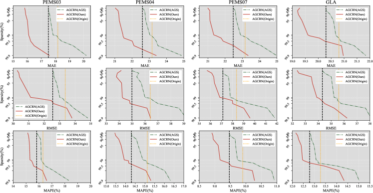
A.5. Additional Experimental Results
Test performances in all metrics of AGCRN and STG-NCDE, localized by DynAGS and AGS across localisation degrees from to , are respectively presented in Figure 6 and Figure 7 for transportation dataset.
A.6. Description of Distributed Simulation
We used Python’s Multiprocessing module to simulate distributed deployment, with each process representing a device. To facilitate and save memory, we created a shared memory ASTGNN model and dataset. It should be noted that in actual deployment, each device is equipped with an ASTGNN model and only has access to the data corresponding to its own nodes before sending communication requests. However, the simulation can still accurately calculate the communication overhead.
A.7. Personalised Localisation Experiment Details
We categorised all nodes into four distinct groups, labeled as \@slowromancapi@, \@slowromancapii@, \@slowromancapiii@, and \@slowromancapiv@. In a personalised setup using DynAGS, these groups achieved in-degree compression ratios of 30%, 50%, 80%, and 99%, respectively.
To draw a meaningful comparison, for each group, we also trained a separate global-localised AGCRN using DynAGS, where every node in the network was subjected to the same in-degree compression ratio specific to that group. For instance, for Group \@slowromancapiii@ with an in-degree compression ratio of 80%, we trained a model where all nodes, regardless of their group, had an in-degree compression ratio of 80%.
The crux of our findings, depicted in Figure 5, is that each group’s performance in the personalised setting mirrored its performance in the corresponding global sparsity setup. For example, the Group \@slowromancapiii@ nodes in the personalised model performed as well as when every node in the system was globally set to an 80% in-degree compression. This demonstrates that the individualised sparsity configurations of other groups did not hinder the performance of any specific group.
In essence, these results affirm that personalising the localisation of ASTGNNs doesn’t compromise performance. Instead, it offers an effective and pragmatic approach.