Computation and Communication Co-scheduling for Timely Multi-Task Inference at the Wireless Edge

Abstract

In multi-task remote inference systems, an intelligent receiver (e.g., command center) performs multiple inference tasks (e.g., target detection) using data features received from several remote sources (e.g., edge sensors). Key challenges to facilitating timely inference in these systems arise from (i) limited computational power of the sources to produce features from their inputs, and (ii) limited communication resources of the channels to carry simultaneous feature transmissions to the receiver. We develop a novel computation and communication co-scheduling methodology which determines feature generation and transmission scheduling to minimize inference errors subject to these resource constraints. Specifically, we formulate the co-scheduling problem as a weakly-coupled Markov decision process with Age of Information (AoI)-based timeliness gauging the inference errors. To overcome its PSPACE-hard complexity, we analyze a Lagrangian relaxation of the problem, which yields gain indices assessing the improvement in inference error for each potential feature generation-transmission scheduling action. Based on this, we develop a maximum gain first (MGF) policy which we show is asymptotically optimal for the original problem as the number of inference tasks increases. Experiments demonstrate that MGF obtains significant improvements over baseline policies for varying tasks, channels, and sources.

I Introduction

The simultaneous advances in machine learning and communication technologies have spurred demand for intelligent networked systems across many domains [1, 2]. These systems, whether for commercial or military purposes, often rely on timely information delivery to a remote receiver for conducting several concurrent decision-making and control tasks [3]. For example, consider intelligence, surveillance, and reconnaissance (ISR) [4] objectives within military operations. A command center may employ signals transmitted from several dispersed military assets, e.g., unmanned aerial vehicles (UAVs), to simultaneously classify friendly versus hostile agents, track the positions of targets, and detect anomalous sensor data. Similarly, in intelligent transportation [5], near real-time prediction of road conditions, vehicle trajectories, and other tasks is crucial for traffic management and safety.

As the number and complexity of learning tasks in such applications continues to rise, there are two salient challenges to facilitating timely multi-task remote inference (MTRI). First, there are limited wireless resources (e.g., orthogonal frequency channels) available for information transmission from sources to the receiver at the network edge. As a result, the sources may locally construct low-dimensional feature representations of their high-dimensional signal observations (e.g., video streams) to send in lieu of the raw measurements. This may be developed, for example, by splitting the neural network for each task at a designated cut layer, and implementing the two parts at the source and receiver, respectively [6]. However, this also leads to the second challenge: the sources, often edge devices, have heterogeneous on-board computational capabilities, limiting their ability to simultaneously construct multiple features required by different tasks. Due to these resource limitations, the features at the receiver may not always reflect the freshest source information.

It is thus critical to ascertain which tasks require feature updates most urgently at any given time, i.e., to determine where to focus available MTRI resources. Age of Information (AoI), introduced in [7, 8], can provide a useful measure of information freshness of the receiver. Specifically, consider packets sent from a source to a receiver: if $U(t)$ is the generation time of the most recently received packet by time $t$, then the AoI at time $t$ is the difference between $t$ and $U(t)$. Recent works on remote inference [9, 3, 10, 11] have shown that the inference errors for different tasks can be expressed as functions of AoI, and that surprisingly, these functions are not always monotonic. Additionally, AoI can be readily tracked in an MTRI system on a per-task basis, making it a promising metric for determining how to prioritize resource allocation.

Motivated by this, we pose the following research question:

How can we develop a computation and communication co-scheduling methodology for MTRI systems that leverages AoI indicators of timeliness to minimize the inference errors across tasks while adhering to network resource constraints?

I-A Outline and Summary of Contributions

• We formulate the MTRI policy optimization problem to minimize discounted infinite horizon inference errors subject to source feature computation and transmission constraints (Sec. II&III-A). This optimization considers the dependency of the inference error on AoI measures for each task’s features and their impact on the prediction results.

• We show how the co-scheduling problem can be modeled as a weakly-coupled Markov Decision Process (MDP) (Sec. III-B). Weakly-coupled MDPs are extensions of restless bandits by allowing for multiple resource constraints. To overcome the associated PSPACE-hard complexity, we derive a Lagrangian relaxation of the original problem, and establish its optimal decision (Sec. IV, Lemma 1). Analyzing the dual problem allows us to obtain a gain index for each task, which quantifies the reduction in inference error from scheduling it.

• Leveraging these gain indices, we propose a novel maximum gain first (MGF) policy to solve the original problem, iteratively scheduling features/tasks with maximum gain until capacity is reached (Sec. V-A). The MGF policy is a special case of the re-optimized fluid (ROF) policy introduced in [12] for general weakly coupled MDPs. We prove that in the MTRI problem, our MGF policy achieves asymptotic optimality at a rate of $O(\frac{1}{\sum_{m=1}^{M}\sqrt{rk_{m}}})$, where $rk_{m}$ is the number of inference tasks per source $m$ and $M$ is the total number of sources (Theorem 1, Sec. V-B). Notably, this optimality gap is tighter than the $O(\frac{1}{\sqrt{\sum_{m=1}^{M}rk_{m}}})$ bound established in [12]. Our scheduling results are applicable to any bounded penalty functions of AoI with multiple resource constraints.

• We conduct numerical experiments to demonstrate our policy on both synthetic and real-world inference tasks (Sec. VI). In the latter case, we consider vehicular inference tasks (image segmentation and traffic prediction) where roadside sensors equipped with cameras are used as the MTRI sources. We find that MGF significantly outperforms baseline policies in terms of cumulative errors as the number of tasks, channels, and sources are varied. A widening margin is observed as the number of tasks increases, consistent with our optimality analysis.

I-B Related Works

AoI has become a widely-used metric in the analysis and optimization of systems including communication networks [13, 14], control systems [15, 16], remote estimation [17, 18, 19], and remote inference [20, 9, 3]. Previous works [20, 9, 3] have demonstrated that the performance of remote inference systems depends on the AoI of the features they utilize; specifically, representing inference error as a function of AoI. In this paper, we consider the more challenging MTRI case with multiple information sources, an edge receiver, and multiple inference tasks for each source. Motivated by the prior work, we consider the dependency of inference error for each task on the AoI of features delivered to the receiver. Notably, the inference error function in our case can be monotonic or non-monotonic with AoI.

Researchers have explored scheduling policies to minimize linear and non-linear functions of AoI in multi-source networked intelligent systems [21, 22, 23, 24, 25, 13, 26, 27, 10, 3, 19]. Early studies focused on systems with limited communication resources and binary actions for each source [21, 22, 23, 24, 25, 13, 26, 27, 19]. More recent research has expanded to consider scenarios with multiple actions per source [10, 3]. These scheduling problems have been formulated as restless multi-armed bandit (RMAB) problems, with either binary or multiple actions. While RMABs are weakly coupled MDPs, which are in general PSPACE-hard, Whittle index [21, 22, 23, 24, 25, 13, 26, 3] and gain index [27, 19, 10] approaches have been shown to yield asymptotically optimal policies under certain conditions, notably the global attractor condition [28, 3, 29]. However, these previous works have not addressed the presence of computation resource constraints and multiple inference tasks characteristic of MTRI systems. By considering these factors, our MTRI computation and communication co-scheduling problem becomes a weakly coupled MDP that is more general than RMAB and requires new approaches to solve it.

Recently, a few works [12, 30] have developed re-optimized fluid policies which are asymptotically optimal for general weakly-coupled MDPs, using linear programming solutions. Our work builds upon the approach provided in [12] to develop scheduling policies for MTRI systems with multiple sources, channels, and inference tasks, which we also show are asymptotically optimal. Importantly, the optimality gap obtained in our paper is tighter than the bound established in [12]. Beyond minimizing inference errors, our gain indicies-based policy is more generally applicable to the minimization of any bounded penalty function of AoI which involves multiple actions per source/task and multiple resource constraints.

II System Model

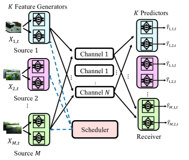
Figure 1: An MTRI system with $M$ sources, $N$ channels, $k_{m}$ feature generators per source $m$ (in this figure, $k_{m}=2$), and $K$ predictors.

II-A Overview

We consider the multi-task remote inference (MTRI) system in Fig. 1. $M$ sources are connected to an intelligent receiver via $N$ wireless channels. For example, in an ISR system, UAVs equipped with cameras can act as sources, transmitting processed video frames to a central command center for further analysis. At every time slot $t$, each source $m$ observes a time-varying signal $X_{m,t}\in\mathcal{X}_{m}$, where $\mathcal{X}_{m}$ represents the set of possible observations, e.g., possible values of video frames captured by a camera. Sources will progressively generate low-dimensional feature representations of their observations for communication-efficient transmission over the $N$ wireless channels when they are scheduled.

At each time $t$, the receiver employs multiple predictors trained to infer targets based on received source features. Specifically, for each source $m$, the receiver aims to infer $k_{m}$ targets $(Y_{m,1,t},Y_{m,2,t},\ldots,Y_{m,k_{m},t})$. These targets can represent various inference tasks, e.g., object detection or segmentation, depending on the nature of the observations and the goals of the MTRI system. In the system, there are a total of $K=\sum_{m=1}^{M}k_{m}$ inference tasks. The tuple $(m,j)$ uniquely identifies the $j$-th inference task of source $m$.

II-B Computation Model

Each source $m$ is equipped with $k_{m}$ pre-trained feature generators. The $j$-th feature generator of source $m$, designed for the $(m,j)$-th inference task, is denoted by a function $\phi_{m,j}:\mathcal{X}_{m}\mapsto\mathcal{Z}_{m,j}$. This function takes the observation $X_{m,t}\in\mathcal{X}_{m}$ as input and generates a feature $F_{m,j,t}=\phi_{m,j}(X_{m,t})\in\mathcal{Z}_{m,j}$, where $\mathcal{Z}_{m,j}$ is the set of possible features generated by $\phi_{m,j}(\cdot)$. To account for computational resource limitations, we assume it is not feasible to activate all feature generators at every time slot. Specifically, for source $m$, at most $C_{m}$ feature generators can be activated at any given time.

II-C Communication Model

As illustrated in Fig. 1, $N$ wireless channels are shared among the $M$ sources. If scheduled at time $t$, the $(m,j)$-th feature generator produces $F_{m,j,t}$ and transmits to the receiver using $n_{m,j}$ channels. For simplicity, we assume perfect channels, i.e., features sent at time slot $t$ are delivered error-free at time slot $t+1$. However, our results can be extended to accommodate erasure channels, where data loss may occur.

Due to the limited number of channels, at any given time $t$, only features for a subset of inference tasks can be transmitted. Consequently, the receiver may not have fresh features for all tasks. If the most recently delivered feature for the $(m,j)$-th inference task was generated $\Delta_{m,j}(t)$ time slots ago, then the feature at the receiver is represented as

$$F_{m,j,t-\Delta_{m,j}(t)}=\phi_{m,j}(X_{m,t-\Delta_{m,j}(t)}),$$

where $\Delta_{m,j}(t)$ is its age of information (AoI) [8, 3]. Let $U_{m,j}(t)$ be the generation time of the most recent delivered feature. Then, the AoI can be formally defined as:

$$\Delta_{m,j}(t)=t-U_{m,j}(t),$$ (1)

which is the difference between the current time $t$ and the generation time $U_{m,j}(t)$.

II-D Inference Model

The receiver is equipped with $K$ pre-trained predictors, where $\psi_{m,j}:\mathcal{Z}_{m,j}\times\mathbb{Z}^{+}\mapsto\mathcal{Y}_{m,j}$ is the predictor function for the $(m,j)$-th inference task. Specifically, predictor $\psi_{m,j}(\cdot,\cdot)$ takes the most recently delivered feature $\phi_{m,j}(X_{m,t-\Delta_{m,j}(t)})\in\mathcal{Z}_{m,j}$ and its AoI $\Delta_{m,j}(t)\in\mathbb{Z}^{+}$ as inputs and generates the predicted result $\hat{Y}_{m,j,t}\in\mathcal{Y}_{m,j}$. In other words, we assume the predictor may in general adjust/calibrate the inference based on the AoI.

We make the following assumptions:

Assumption 1.

The processes $\{(Y_{m,j,t},X_{m,t}),t=0,1,\ldots\}$ and $\{\Delta_{m,j}(t),t=0,1,\ldots\}$ are independent for all $(m,j)$.

Assumption 2.

The process $\{(Y_{m,j,t},X_{m,t}),t=0,1,\ldots\}$ is stationary for all $(m,j)$, i.e., the joint distribution of $(Y_{m,j,t},X_{m,t-k})$ does not change over time $t$ for all $k\geq 0$.

Assumption 1 is satisfied for signal-agnostic scheduling policies in which the scheduling decisions are made based on AoI and the distribution of the process, but not on the values taken by the process [3]. Assumption 2 is utilized to ensure that the inference error is a time-invariant function of the AoI, as we will see in (II-D). It is practical to approximate time-varying functions as time-invariant functions in the scheduler design. Moreover, the scheduling policy developed for time-invariant AoI functions serves as a valuable foundation for studying time-varying AoI functions [31].

Under Assumptions 1-2, given an AoI $\Delta_{m,j}(t)=\delta$, the inference error for the $(m,j)$-th inference task at time slot $t$ can be represented as a function of AoI $\delta$ [3, 9]:

$$p_{m,j}(\delta)$$

$$=\mathbb{E}_{Y,X\sim P_{Y_{m,j,t},X_{m,t-\delta}}}\bigg{[}L_{m,j}(Y,\psi_{m,j}(\phi_{m,j}(X),\delta))\bigg{]},$$ (2)

where $P_{Y_{m,j,t},X_{m,t-\delta}}$ is the joint distribution of the target $Y_{m,j,t}$ and the observation $X_{m,t-\delta}$, and $L_{m,j}(y,\hat{y})$ is the loss function for the task that measures the loss incurred when the actual target is $y$ and the inference result is $\hat{y}$ (e.g., cross-entropy loss for a classification task).

III Scheduling Problem Formulation

III-A Scheduling Policy and Optimization

We denote the scheduling policy as

$$\pi=(\pi_{m,j}(0),\pi_{m,j}(1),\ldots)_{\forall(m,j)},$$

where $\pi_{m,j}(t)\in\{0,1\}$. At time slot $t$, if $\pi_{m,j}(t)=1$, the features for the $(m,j)$-th inference task are generated and transmitted to the receiver; otherwise, if $\pi_{m,j}(t)=0$, this generation and transmission does not occur. We let $\Pi$ denote the set of all signal-agnostic and causal scheduling policies $\pi$ that satisfy three conditions: (i) the scheduler knows the AoIs up to the present time, i.e., $\{\Delta_{m,j}(k)\}_{\forall m,j,k\leq t}$, (ii) the scheduler does not know signal values $\{X_{m,t},Y_{m,j,t}\}_{\forall m,j,t}$, and (iii) the scheduler has access to the inference error functions $p_{m,j}(\delta)$ for all $(m,j)$.

Under any scheduling policy $\pi$, the AoI $\Delta_{m,j}(t)$ for each inference task $(m,j)$ evolves according to:

$$\!\!\Delta_{m,j}(t+1)=\begin{cases}1,&\text{if}~\pi_{m,j}(t)=1\\ \Delta_{m,j}(t)+1,&\text{otherwise}.\end{cases}$$ (3)

We assume that the initial AoI of each task $(m,j)$ is a finite constant, e.g., $\Delta_{m,j}(0)=1$.

Our goal is to find a policy $\pi\in\Pi$ that minimizes the infinite horizon discounted sum of inference errors over the $K$ tasks:

$$\bar{p}_{opt}=$$

$$\;\inf_{\pi\in\Pi}\sum_{t=0}^{\infty}\frac{\gamma^{t}}{K}\sum_{m=1}^{M}\sum_{j=1}^{k_{m}}\mathbb{E}_{\pi}\left[w_{m,j}p_{m,j}(\Delta_{m,j}(t))\right],$$ (4)

$$~\mathrm{s.t.}\sum_{j=1}^{k_{m}}\pi_{m,j}(t)\leq C_{m},t=0,1,\ldots,m=1,\ldots,M,$$ (5)

$$~~~~\sum_{m=1}^{M}\sum_{j=1}^{k_{m}}\pi_{m,j}(t)n_{m,j}\leq N,~~t=0,1,2,\ldots,$$ (6)

where $w_{m,j}\geq 0$ is the weight (e.g., priority) associated with the $(m,j)$-th inference task, and the discount factor $0<\gamma<1$ quantifies the diminishing importance of an inference task over time. At most $C_{m}$ feature generators for source $m$ can compute features at time $t$. Transmitting features for the $(m,j)$-th inference task requires $n_{m,j}$ of the $N$ wireless channels available. For each task, its inference error, $p_{m,j}(\Delta_{m,j}(t))$, depends on its AoI $\Delta_{m,j}(t)$ at time slot $t$, indicating the freshness of the feature used for inference.

III-B Weakly Coupled MDP Formulation

The problem (III-A)-(6) is a weakly coupled Markov decision process (MDP) [12, 30, 32] with $K$ sub-MDPs (referred to as arms in the bandit literature), one per inference task $(m,j)$ across sources $m$. The state of each $(m,j)$-th MDP at each time $t$ is represented by the AoI $\Delta_{m,j}(t)$. The action is $\pi_{m,j}(t)$, and its per-timeslot cost is $\gamma^{t}p_{m,j}(\Delta_{m,j}(t))$ with discount factor $0<\gamma<1$. We can see that the state evolution defined in (3) and the cost of each MDP depends only on its current state and action. However, the actions for all MDPs $(\pi_{m,j}(t))_{\forall m,j}$ need to satisfy the constraints in (5)-(6). This interdependence of actions across MDPs through multiple resource constraints, despite independent state transitions and costs, makes the overall problem (III-A)-(6) a weakly coupled MDP [12, 30, 32]. Weakly coupled MDPs are PSPACE-hard because the number of states and actions grow exponentially with the number of sub-MDPs.

The restless multi-armed bandit (RMAB) problem is a special case of the weakly coupled MDP in (III-A)-(6). RMAB considers a single resource constraint, whereas our problem involves multiple resource constraints (5)-(6). The PSPACE-hard complexity of RMABs can be overcome by using Whittle indices [28, 9, 3, 24, 21, 33, 26], gain indices [10, 19, 27], and linear programming-based indices [34] to construct asymptotically optimal policies, provided indexability and/or global attractor conditions are satisfied. However, these RMAB policies cannot be directly applied to our more general problem due to the presence of multiple resource constraints, which requires us to develop a new solution approach.

Solution approach. In Sec. IV&V, we follow the approach depicted in Fig. 2 to solve (III-A)-(6). We begin by deriving a relaxed Lagrangian problem. We then utilize the resulting solution to construct a maximum gain first (MGF) policy (Algorithm 1) for (III-A)-(6). Theorem 1 will demonstrate that the MGF policy becomes asymptotically optimal as the number of inference task $k_{m}$ for each source $m$ increases.

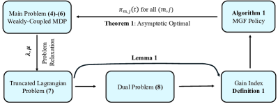
Figure 2: Overview of our process to design the scheduling policy.

IV Problem Relaxation

IV-A Lagrangian Relaxation and Dual Problem

To develop an asymptotically optimal policy for (III-A)-(6), following recent techniques for weakly coupled MDPs [32, 12], we first relax the problem using Lagrange multipliers. We associate a vector of non-negative Lagrange multipliers $\boldsymbol{\lambda}_{t}=(\lambda_{1,t},\lambda_{2,t},\ldots,\lambda_{M,t})$ with constraints (5) and a non-negative Lagrange multiplier $\mu_{t}$ with constraint (6) at each time $t$. To avoid an infinite number of Lagrange multipliers associated with the constraints over the infinite time horizon from $t=0$ to $t=\infty$, we truncate the problem to a finite time horizon $T$ as shown in (IV-A). Due to bounded inference error function, the performance loss resulting from this truncation becomes negligible for sufficiently large values of $T$.

The truncated problem is given by

$$\bar{p}(\boldsymbol{\lambda},\boldsymbol{\mu};\tau:T)=$$

$$\;\inf_{\pi\in\Pi}\sum_{t=\tau}^{T}\sum_{m=1}^{M}\sum_{j=1}^{k_{m}}\frac{\gamma^{t}\mathbb{E}_{\pi}\left[w_{m,j}p_{m,j}(\Delta_{m,j}(t))\right]}{K}$$

$$+\sum_{t=\tau}^{T}\sum_{m=1}^{M}{\lambda_{m,t}}\frac{\gamma^{t}}{K}\left(\left(\sum_{j=1}^{k_{m}}\pi_{m,j}(t)\right)-C_{m}\right)$$

$$+\sum_{t=\tau}^{T}{\mu_{t}}\frac{\gamma^{t}}{K}\left(\left(\sum_{m=1}^{M}\sum_{j=1}^{k_{m}}\pi_{m,j}(t)n_{m,j}\right)-N\right),$$ (7)

where $\boldsymbol{\lambda}=(\boldsymbol{\lambda}_{\tau},\boldsymbol{\lambda}_{\tau+1},\ldots,\boldsymbol{\lambda}_{T})$, $\boldsymbol{\mu}=(\mu_{0},\mu_{1},\ldots,\mu_{T})$, $\bar{p}(\boldsymbol{\lambda},\boldsymbol{\mu};\tau:T)$ is the optimal value of (IV-A), and $\tau=0,1,\ldots,T$.

The dual problem to (IV-A) is given by

$$(\boldsymbol{\lambda}^{*},\boldsymbol{\mu}^{*})=\operatorname*{arg\,max}_{(\boldsymbol{\lambda},\boldsymbol{\mu})\geq 0}\bar{p}(\boldsymbol{\lambda},\boldsymbol{\mu};\tau:T),$$ (8)

where $(\boldsymbol{\lambda}^{*},\boldsymbol{\mu}^{*})$ is the optimal dual solution.

IV-B Optimal Solution to (IV-A)

The problem (IV-A) can be decomposed into $K$ sub-problems, one per task, in which the $(m,j)$-th sub-problem is given by

$$\bar{p}_{m,j}(\boldsymbol{\lambda}_{m},\boldsymbol{\mu};\tau:T)$$

$$= \inf_{\pi_{m,j}\in\Pi_{m,j}}\sum_{t=\tau}^{T}\gamma^{t}\mathbb{E}_{\pi_{m,j}}\bigg{[}w_{m,j}p_{m,j}(\Delta_{m,j}(t))$$

$$+\lambda_{m,t}\pi_{m,j}(t)+\mu_{t}\pi_{m,j}(t)n_{m,j}\bigg{]},$$ (9)

where $\bar{p}_{m,j}(\boldsymbol{\lambda}_{m},\mu;\tau:T)$ is the optimal objective value of the sub-problem, $\boldsymbol{\lambda}_{m}=(\lambda_{m,\tau},\lambda_{m,\tau+1},\ldots,\lambda_{m,T}),$ $\pi_{m,j}=(\pi_{m,j}(\tau),\ldots,\pi_{m,j}(T))$ is a scheduling policy for the task, and $\Pi_{m,j}$ is the set of all causal signal-ignorant policies. The Lagrange multipliers $\boldsymbol{\lambda}_{m}$ and $\boldsymbol{\mu}$ correspond to the computation cost and the communication cost terms, respectively.

By solving the sub-problem (IV-B) for each $(m,j)$-th MDP and combining the solutions, we get an optimal policy for (IV-A). Following this approach, we present an optimal policy to the sub-problem (IV-B) in Lemma 1.

Lemma 1.

There exists an optimal policy for (IV-B) in which the optimal decision $\pi^{*}_{m,j}(t)$ at each time $t$ is determined by

$$\pi^{*}_{m,j}(t)=\operatorname*{arg\,min}_{\pi_{m,j}(t)\in\{0,1\}}Q^{\boldsymbol{\lambda}_{m},\boldsymbol{\mu}}_{m,j,t}(\Delta_{m,j}(t),\pi_{m,j}(t)),$$ (10)

where the action value function $Q^{\boldsymbol{\lambda}_{m},\boldsymbol{\mu}}_{m,j,t}(\cdot,\cdot)$ is given by

$$Q^{\boldsymbol{\lambda}_{m},\boldsymbol{\mu}}_{m,j,t}(\delta,a) =w_{m,j}p_{m,j}(\delta)+(1-a)\gamma V^{\boldsymbol{\lambda}_{m},\boldsymbol{\mu}}_{m,j,t+1}(\delta+1)$$

$$+a\left(\lambda_{m,t}+\mu_{t}n_{m,j}+\gamma V^{\boldsymbol{\lambda_{m}},\boldsymbol{\mu}}_{m,j,t+1}(1)\right),$$ (11)

the value function $V^{\boldsymbol{\lambda}_{m},\boldsymbol{\mu}}_{m,j,t}(\cdot)$ for all $\delta\in\mathbb{Z}^{+}$ and $t=\tau,\tau+1,\ldots,T$ is given by

$$V^{\boldsymbol{\lambda}_{m},\boldsymbol{\mu}}_{m,j,t}(\delta)=\min_{a\in\{0,1\}}Q^{\boldsymbol{\lambda}_{m},\boldsymbol{\mu}}_{m,j,t}(\delta,a),$$ (12)

and for $t=T+1,$

$$V^{\boldsymbol{\lambda}_{m},\boldsymbol{\mu}}_{m,j,T+1}(\delta)=0.$$ (13)

Proof.

The action $\pi^{*}_{m,j}(t)$ is optimal because it satisfies the Bellman optimality equation [35, 36]:

$$\!\!\!\!\!V^{\boldsymbol{\lambda}_{m},\boldsymbol{\mu}}_{m,j,t}(\delta)$$

$$\!\!=\min_{a\in\{0,1\}}w_{m,j}p_{m,j}(\delta)+a\left(\lambda_{m,t}+\mu_{t}n_{m,j}\right)$$

$$\!\!\!\!\!+\gamma\mathbb{E}\!\left[V^{\boldsymbol{\lambda}_{m},\boldsymbol{\mu}}_{m,j,t+1}(\Delta_{m,j}(t+1))\bigg{|}\Delta_{m,j}(t)\!=\!\delta,\!\pi_{m,j}(t)\!=a\!\right].$$ (14)

∎

Lemma 1 establishes an optimal decision $\pi^{*}_{m,j}(t)$ for problem (IV-B) by using dynamic programming method. The backward induction method to compute the value function $V^{\boldsymbol{\lambda}_{m},\boldsymbol{\mu}}_{m,j,t}(\delta)$ for $t=\tau,\tau+1,\ldots,T$ is given by

$$V^{\boldsymbol{\lambda}_{m},\boldsymbol{\mu}}_{m,j,t}(\delta)\! =\!w_{m,j}p_{m,j}(\delta)+\!\min_{a\in\{0,1\}}\bigg{\{}\!(1-a)\gamma V^{\boldsymbol{\lambda}_{m},\boldsymbol{\mu}}_{m,j,t+1}(\delta+1)$$

$$+a\left(\lambda_{m,t}+\mu_{t}n_{m,j}+\gamma V^{\boldsymbol{\lambda}_{m},\boldsymbol{\mu}}_{m,j,t+1}(1)\right)\bigg{\}}.$$ (15)

However, if the AoI $\delta$ can take infinite values, this is computationally intractable. Thus, we restrict the computation of value function to a finite range $\delta=1,2,\ldots,\bar{\delta}$, and approximate $V^{\boldsymbol{\lambda}_{m},\boldsymbol{\mu}}_{m,j,t}(\delta)\approx V^{\boldsymbol{\lambda}_{m},\boldsymbol{\mu}}_{m,j,t}(\bar{\delta})$ for values exceeding this range. In reality, this truncation will have a negligible effect since (i) higher AoI values are rarely visited in practice [37], and (ii) the inference error $p_{m,j}(\delta)$ tends to converge to an upper bound as AoI becomes large, as seen in some recent works [3, 9, 10] and our machine learning experiments in Fig. 4. The backward induction algorithm has a time complexity of $O(\bar{\delta}T)$.

IV-C Solution to (8)

Next, we solve the dual problem (8). We can reformulate the dual problem as

$$\max_{\boldsymbol{\lambda}\geq 0,\boldsymbol{\mu}\geq 0} \sum_{t=\tau}^{T}\sum_{m=1}^{M}\sum_{j=1}^{k_{m}}V^{\boldsymbol{\lambda}_{m},\boldsymbol{\mu}}_{m,j,t}(\Delta_{m,j}(t))$$

$$-\sum_{t=\tau}^{T}\sum_{m=1}^{M}\gamma^{t-\tau}\lambda_{m,t}C_{m}+\sum_{t=\tau}^{T}\gamma^{t-\tau}\mu_{t}N,$$ (16)

where $V^{\boldsymbol{\lambda}_{m},\boldsymbol{\mu}}_{m,j,t}(\Delta_{m,j}(t))$ is obtained by using (IV-B).

V Scheduling Policy

V-A Maximum Gain First (MGF) Scheduler

While the decision $\pi^{*}_{m,j}(t)$ provided in Lemma 1 may violate constraints (5)-(6), we exploit the structure of the decision $\pi^{*}_{m,j}(t)$ to develop a scheduling policy for the original problem (III-A)-(6). The proposed policy utilizes the notion of gain indices discussed in some recent papers [3, 19, 27]. To determine gain indices for our MTRI problem at time $t$, we use the action value function $Q^{\boldsymbol{\lambda}^{*}_{m},\boldsymbol{\mu}^{*}}_{m,j,t}(\cdot)$ associated with Lagrange multipliers $\lambda^{*}_{m,t},\lambda^{*}_{m,t+1},\ldots,\lambda^{*}_{m,T}$ and $\mu^{*}_{t},\mu^{*}_{t+1},\ldots,\mu^{*}_{T}$.

Definition 1 (Gain Index).

[3] Given an AoI value $\Delta_{m,j}(t)=\delta$, the gain index $\alpha_{m,j,t}(\delta)$ for the $(m,j)$-th task at time $t$ is the difference of two actions values, determined by

$$\alpha_{m,j,t}(\delta)=Q^{\boldsymbol{\lambda}^{*}_{m},\boldsymbol{\mu}^{*}}_{m,j,t}(\delta,0)-Q^{\boldsymbol{\lambda}^{*}_{m},\boldsymbol{\mu}^{*}}_{m,j,t}(\delta,1),$$ (17)

where $(\boldsymbol{\lambda}^{*}_{m},\boldsymbol{\mu}^{*})$ is an optimal solution to (IV-A) after substituting $\tau=t$ in (IV-A).

The gain index $\alpha_{m,j,t}(\delta)$ quantifies the discounted total reduction in inference errors when action $\pi_{m,j}(t)=1$ is chosen over $\pi_{m,j}(t)=0$, where the latter implies no resource allocation for the $(m,j)$-th inference task at time $t$. This metric enables strategic resource utilization at each time slot to enhance overall system performance.

Algorithm 1 presents our maximum gain first (MGF) scheduler for solving the main problem (III-A)-(6). At each time $t$, the policy $\pi_{\text{MGF}}$ prioritizes generating and transmitting features ($\pi_{m,j}(t)=1$) for the inference tasks with highest gain index, while adhering to the available communication and computation resources. Formally, at time $t$, let

$$A(t)=\bigg{\{}(m,j):\alpha_{m,j,t}(\Delta_{m,j}(t))>0\bigg{\}}$$ (18)

be the set of inference tasks with positive gain indices. Our policy then proceeds as follows:

• Select the inference task $(m^{*},j^{*})$ that satisfies

  $$(m^{*},j^{*})=\operatorname*{arg\,min}_{(m,j)\in A(t)}\alpha_{m,j,t}(\Delta_{m,j}(t)).$$ (19)

  Source $m^{*}$ generates and transmits its features for the $(m^{*},j^{*})$-th inference task, provided that the resource budget has not been exhausted.

• Remove the tuple $(m^{*},j^{*})$ from $A(t)$, i.e., $A(t)=A(t)\setminus(m^{*},j^{*})$. Repeat (1) until the set $A(t)$ is empty.

Comparing (10), (17), and (19), we observe that our policy closely approximates the optimal solution to the Lagrangian relaxed problem (IV-A), aiming to make as close to full use of the resource constraints as possible.

V-B Performance Analysis

We now analyze the performance of our policy relative to the original problem (III-A)-(6). Following standard practice in the weakly-coupled MDP literature [12, 30], we consider a set of sub-problems at source $m$ to be in the same class if they share identical penalty functions, weights, and transition probabilities, where each sub-problem is indexed by the $(m,j)$-th inference task.

Definition 2 (Asymptotic optimality).

Consider a “base” MTRI system with $N$ channels, $M$ sources, $k_{m}$ classes of sub-problems per source $m$, and a computation resource budget $C_{m}$ for source $m$. Let $\bar{p}^{r}_{{\text{MGF}}}$ represent the discounted infinite horizon sum of inference errors under policy $\pi_{\text{MGF}}$ for a system with computation resource budget $rC_{m}$, communication resource budget $rN$, and $k_{m}$ classes of sub-problems per source $m$ in which each class of sub-problems contain $r$ inference tasks while maintaining a constant $M$ sources. The policy $\pi_{\text{MGF}}$ is asymptotically optimal if $\bar{p}^{r}_{{\text{MGF}}}=\bar{p}_{{\pi}^{r}_{opt}}$ for all $\pi\in\Pi$ as inference task per class $r$ approaches $\infty$.

First, we provide Lemma 2, which is a key tool to showing asymptotic optimality. Let the policy $\pi^{*}=(\pi^{*}_{m,j}(t))_{\forall m,j,t\leq T}$ be an optimal solution to (IV-A), where the action $\pi^{*}_{m,j}(t)$ is obtained by using Lemma 1 and by getting the optimal Lagrange multipliers of (8) with $\tau=t$. Using (10) and (17), we can verify that $\pi^{*}_{m,j}(t)=1$ if and only if $\alpha_{m,j,t}(\Delta_{m,j}(t))>0$.

Lemma 2.

For any time $t$ and AoI values, the expected number of inference tasks $(m,j)$ with different actions under the MGF policy and the policy $\pi^{*}$ is bounded above by $\sum_{m=1}^{M}\sqrt{k_{m}}+\sqrt{\sum_{m=1}^{M}k_{m}}$.

Proof.

See Appendix A. ∎

Then, we can obtain our main theoretical result:

Theorem 1.

If the weighted functions $w_{m,j}p_{m,j}(\delta)$ are bounded for all tasks $(m,j)$ and

$$T\geq\log_{\frac{1}{\gamma}}\left(\sum_{m=1}^{M}\sqrt{rk_{m}}\right),$$ (20)

then the MGF policy is asymptotically optimal as the number of inference tasks $r$ per class of sub-problems increases. Specifically, we have

$$\bar{p}^{r}_{{\text{MGF}}}-\bar{p}^{r}_{\text{opt}} \leq\frac{1}{\sum_{m=1}^{M}\sqrt{rk_{m}}}\left(\frac{2M(\bar{p}_{h}-\bar{p}_{l})\gamma}{(1-\gamma)^{3}}+\frac{(\bar{p}_{h}-\bar{p}_{l})\gamma}{(1-\gamma)}\right)$$

$$=O\bigg{(}\frac{1}{\sum_{m=1}^{M}\sqrt{rk_{m}}}\bigg{)},$$ (21)

where $k_{m}$ is the number of sub-problems per source, $M$ is the number of sources, $\gamma$ is the discount factor, and $\bar{p}_{h}$ and $\bar{p}_{l}$ are finite constants such that $\bar{p}_{l}\leq w_{m,j}p_{m,j}(\delta)\leq\bar{p}_{h}$ for any sub-problem $(m,j)$ and AoI value $\delta=1,2,\ldots.$

Proof.

See Appendix B. ∎

According to Theorem 1 and Definition 2, our policy approaches the optimal as the number of inference tasks $r$ per class of sub-problems increases asymptotically.

While prior work has introduced gain-index-based policies for RMAB problems [19, 27, 10], these cannot be directly applied to general weakly-coupled MDPs. Our gain-index-based policy, a specialized re-optimized fluid policy (Definition 3) [12], achieves tighter asymptotic optimality for MTRI systems (see (1)) compared to the $O(\frac{1}{\sqrt{\sum_{m=1}^{M}rk_{m}}})$ bound in [12]. This improvement is obtained by using Lemma 2, which strengthens the result [12, Lemma EC1.1] by exploiting the MTRI constraint structure: sub-problems utilize only their source’s computational resources. Unlike the general system in [12] where all resources are globally shared, MTRI systems have local (computational) and global (communication) resources, yielding a tighter bound. For example, a sub-problem associated with source $m_{1}$ would only consume computational resources from source $m_{1}$ and not from another source $m_{2}$, unlike in [12], where all sub-problems share all resources in the system.

1 for $t=0,1,\ldots$ do

2   Update $\Delta_{m,j}(t)$ for all $(m,j)$

3    Initialize $\pi_{m,j}(t)\leftarrow 0$ for all $(m,j)$

4    Get $\boldsymbol{\lambda}^{*}$ and $\mu^{*}$ that maximizes $\bar{p}(\boldsymbol{\lambda},\boldsymbol{\mu};t:T)$

5    $\alpha_{m,j}\leftarrow\alpha_{m,j,t}(\Delta_{m,j}(t))$ for all $(m,j)$

6    $C_{m,\text{curr}}\leftarrow 0$ and $N_{\text{curr}}\leftarrow 0$

7    $A(t)\leftarrow\{(m,j):\alpha_{m,j}>0)\}$

8    while $A(t)$ is not empty do

9       $(m^{*},j^{*})\leftarrow\operatorname*{arg\,max}_{m,j}\alpha_{m,j}$

10       $c\leftarrow C_{m^{*},\text{curr}}+1$ and $n\leftarrow N_{\text{curr}}+n_{m^{*},j^{*}}$

11       if $c\leq C_{m^{*}}$ and $n\leq N$ then

12         Update $\pi_{m^{*},j^{*}}(t)\leftarrow 1$

13          Update $C_{m^{*},\text{curr}}\leftarrow c$ and $N_{\text{curr}}\leftarrow n$

14      $A(t)=A(t)\setminus(m^{*},j^{*})$

Algorithm 1 Maximum Gain First (MGF) Policy

VI Numerical Experiments

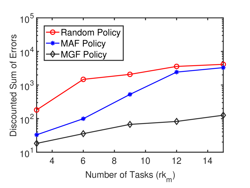
(a) Dis. Sum of Errors vs. $rk_{m}$

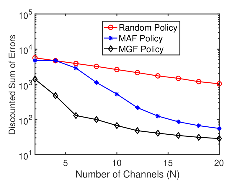
(b) Dis. Sum of Errors vs. $N$

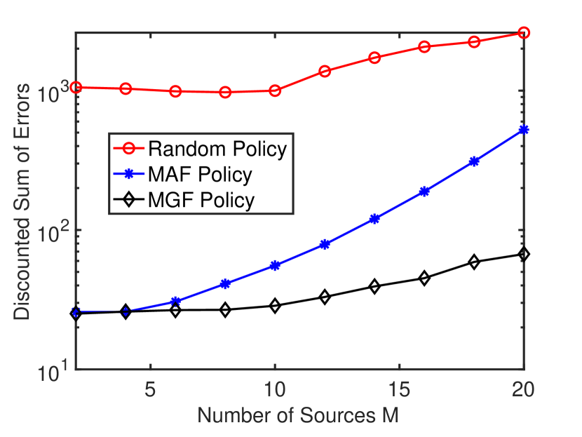
(c) Dis. Sum of Errors vs. $M$

Figure 3: Model-based evaluations: (a) discounted sum of errors vs. number of tasks per source $rk_{m}$, (b) discounted sum of errors vs. number of channels $N$, and (c) discounted sum of errors vs. number of sources $M$. The MGF policy has the potential to achieve a discounted sum of inference errors up to 26 and 32 times lower than the MAF and Random policies, respectively.

We consider the following three policies for evaluation:

• Maximum Gain First (MGF) Policy: The scheduling decision under this policy follows Algorithm 1.

• Maximum Age First (MAF) Policy: At each time slot $t$, the MAF policy selects the inference task $(m,j)$ with the highest AoI from the set of all inference tasks $A_{1}(t)$ with non-zero AoI. If constraints permit, the policy generates and transmits the feature for the selected task. Then, $(m,j)$ is removed from $A_{1}(t)$. This process repeats until $A_{1}(t)$ is empty. AoI-based priority policies are commonly used as baselines in the literature [38, 3, 39].

• Random Policy: At each time slot $t$, the random policy selects one inference task $(m,j)$ from the set of all tasks $A_{2}(t)$ following a uniform distribution. If constraints permit, the policy generates and transmits the feature for the selected task. The task $(m,j)$ is then removed from $A_{2}(t)$. This process repeats until $A_{2}(t)$ becomes empty.

We evaluate these three policies under two scenarios:

• Synthetic evaluations: We assess the policies assuming synthetic AoI penalty functions for all inference tasks (Sec. VI-A).

• Real-world evaluations: We conduct two machine learning experiments and incorporate the resulting inference error functions into the simulation (Sec. VI-B).

VI-A Synthetic Evaluations

In this section, we use three AoI penalty functions: $p_{m,j}(\delta)=\delta,\exp(0.5\delta),10\text{log}(\delta)$. Each function is assigned to one-third of the inference tasks in each source $m$.

Fig. 3(a) illustrates the discounted sum of inference errors versus the number of tasks per source ($rk_{m}$) over a time horizon of $T=100$. Referring to Definition 2, we set $k_{m}=3$ and vary $r$. The additional simulation parameters are $M=20$, $N=10$, $\gamma=0.9$, $n_{m,j}=1$ for all tasks $(m,j)$, $C_{m}=2$ for all sources $m$, and $w_{m,j}=0.01$ for half of the tasks and $1$ for the other half. We see that, when $rk_{m}=15$, the total discounted penalty for the MAF policy is $26$x higher than that of the MGF policy, while the random policy incurs $32$x higher penalty. The performance of the MAF policy deteriorates more rapidly than the MGF policy as the number of tasks per source increases, aligning with our findings in Theorem 1.

In Fig. 3(b), we plot the discounted sum of errors against the number of channels $N$. Here, $k_{m}=3$ and $r=3$ for each source $m$, and the rest of the parameters are the same as in Fig. 3(a). We see that increasing $N$ improves performance for all policies, but more rapidly for MGF. When $N=2$, the MAF policy incurs four times penalty of the MGF policy. This performance gap narrows as $N$ increases, but even with $N=20$, the MAF policy’s inference error remains twice that of the MGF policy.

In Fig. 3(c), we plot the discounted sum of errors against the number of sources $M$, with other parameters the same as in Fig. 3(a)&(b). As the number of sources increases, we see that the performance gap between MAF and MGF policies widens. This shows that MGF is more effective as the number of sources competing for MTRI resources increases.

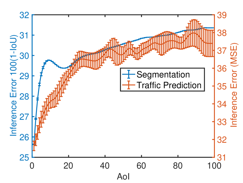
(a) Inference Error vs AoI

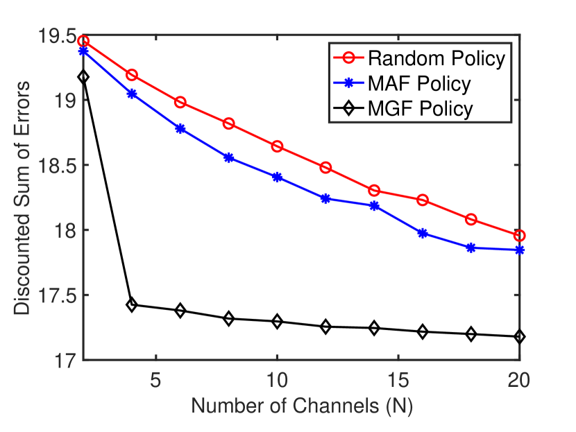
(b) Dis. Sum of Errors vs. $N$

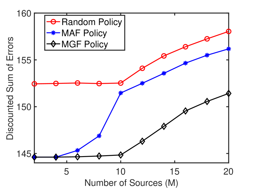
(c) Dis. Sum of Errors vs. $M$

Figure 4: Data-driven evaluations: (a) Inference error vs. AoI for segmentation task (left), where we use 100 (1-IoU) loss function, and for traffic prediction (right), where we use quadratic loss function. (b) Discounted sum of errors vs. number of channels $N$ in which two inference tasks are given priority with weight $1$ and the others have weight $0.01$. (c) Discounted sum of errors vs. number of sources $M$ in which half of the inference tasks given priority with weight $1$ and the others have weight $0.01$. MGF outperforms the other two policies.

VI-B Real-World Evaluations

VI-B1 Machine Learning Experiments

We consider two machine learning tasks: (i) scene segmentation and (ii) traffic prediction. To collect the inference error functions, we employ the NGSIM dataset [40, 41, 42, 43], which contains video recordings from roadside unit (RSU) cameras installed above four different US road surfaces. These videos capture traffic from various camera angles around the road surfaces and were recorded at different times of the day, each for a duration of 15 minutes.

In our experiments, each source is modeled as an RSU. Each RSU generates features for the two inference tasks: video frame segmentation and traffic prediction. We define a time slot as the duration of two video frames, during which feature generation and transmission are completed. We randomly select $4$ videos for our analysis.

Scene Segmentation: For image segmentation, we utilize the Segment Anything Model (SAM) released by Meta AI [44]. We adopt the medium ViT-L model as a pre-trained model to segment each frame into distinct areas. We split the ViT-L model into two parts: a feature generator and a predictor. The predictor model takes feature generated at time $t-\delta$ as input to predict the segmentation for frame at time $t$, where $\delta$ is the AoI value. By taking feature produced at time $t$, we generate ground truth for loss calculation. We employ the Intersection over Union 100(1-IoU) loss metric, where $\text{IoU}=\frac{\hat{S}\cap S}{\hat{S}\cup S}$, $S$ is the ground truth segmentation of the frame containing combined masks for all distinct segments, and $\hat{S}$ is the predicted segmented frame. We use the loss function over the selected videos from the dataset to generate inference error.

Traffic Prediction: For traffic prediction, we leverage image pre-processing techniques and pre-trained state-of-the-art (SOTA) models. Each frame is duplicated, with one copy undergoing SAM-based segmentation mask application and the other undergoing grayscaling, edge enhancement, resizing, and blurring. Both processed frames are then fed into a pre-trained YOLOv8 [45] image detection model to identify all vehicles. The detected vehicles from both frames are combined, removing any overlaps, and their positions are saved, creating the final data sequences. Combined SAM-YOLOv8 model, along with pre-processing, serves as feature generator.

After generating the data sequences, we split them into 80% training and 20% inference datasets. Our prediction framework utilizes a separate LSTM model for each AoI value $\delta$, with hyperparameters detailed in Table I. For a given AoI $\delta$, the input to the corresponding LSTM model is the sequence of vehicle counts from $\delta-l$ to $\delta$ frames ago, with the goal of predicting the current vehicle count. We train each model for $50$ epochs. Using the trained LSTM models, we record inference errors for each AoI $\delta=1,2,\dots,100$.

Hyperparameter	Value
Hidden Layers	16
Input and Output Size	1
Batch Size	32
Window Size ($l$)	3
Optimizer	Adam
Learning Rate	0.0001

TABLE I: Hyperparameters used for the LSTM models.

Fig. 4(a) illustrates the resulting inference errors vs. AoI.

VI-B2 Evaluations of Scheduling Policies

We now evaluate the scheduling policies employing these inference error functions. In Fig. 4(b), we plot the discounted sum of errors against the number of channels $N$ over a time horizon of $T=100$, with two inference tasks $k_{m}=2$ per source and scaling factor $r=1$. We set $M=20$, $\gamma=0.9$, $n_{m,j}=1$, and $C_{m}=2$ for all sources. Task weights $w_{m,j}$ are set to 1 for tasks (1,2) and (5,1), and 0.01 for the rest. As expected, increasing $N$ is seen to improve performance across all policies. Notably, when $N=4$, the MGF policy outperforms the MAF policy by $10\%$. Additionally, Fig. 4(b) clearly demonstrates the consistently poor performance of the random policy.

Fig. 4(c) illustrates the performance of the scheduling policies as the number of sources $M$ increases, over a finite horizon of $T=100$. Each source has two inference tasks $k_{m}=2$ and $r=1$, with other simulation parameters set to $N=10$, $\gamma=0.9$, $n_{m,j}=1$, and $C_{m}=1$. We assign weights $w_{m,j}$ of $1$ to half the inference tasks and $0.01$ to the rest. We see that while the MAF and MGF policies perform similarly with a small number of sources, the MGF policy becomes better as the number of sources increases.

VI-C Discussion

Synthetic evaluations (Sec. VI-A) demonstrate that the MGF policy significantly outperforms both the MAF and random policies, achieving up to 26x and 32x better performance, respectively. The improvement is particularly evident as the number of tasks per source increases, thus validating Theorem 1. Real-world data-driven evaluations (Sec. VI-B) further confirm the MGF policy’s superiority, though the gains are not as high as the gains achieved in synthetic evaluations. This is due to limitations in the inference tasks, specifically, the small number of tasks per source (only 2) and the small variation in the inference error functions as AoI increases (Fig. 4(a)). This limited variation is attributed to the dataset’s unchanging background scene and consistent number of vehicles over time. However, with more tasks or greater variability in inference difficulty, MGF’s advantage would be expected to increase. In scenarios where feature freshness impacts inference difficulty, MGF’s adaptability will be especially beneficial. Under such conditions, MGF’s performance gains should approach those seen in synthetic evaluations. Overall, the simulation results highlight strong performance of the MGF policy compared to baselines.

VII Conclusion

In this paper, we studied the problem co-scheduling computation and communication in MTRI systems to minimize inference errors under resource constraints. We formulated this problem as a weakly-coupled MDP with inference errors described as penalty functions of AoI. To address the resulting PSPACE-hard complexity, we developed a novel MGF policy, which our theoretical analysis proved to be asymptotically optimal as the number of inference tasks increases. Numerical evaluations using both synthetic and real-world datasets further validated MGF’s superior performance compared to baseline policies.

Appendix A Proof of Lemma 2

In this proof, we use $n_{m,j}=1$ for the simplicity of analysis. Denote $\pi^{\text{MGF}}_{m,j}(t)$ as the action under MGF policy. Define

$$I_{t}=\bigg{\{}(m,j):\pi^{\text{MGF}}_{m,j}(t)\neq\pi^{*}_{m,j}(t)\bigg{\}},$$

$$C^{*}_{m}(t)=\sum_{j=1}^{k_{m}}\pi^{*}_{m,j}(t),N^{*}(t)=\sum_{m=1}^{M}\sum_{j=1}^{k_{m}}\pi^{*}_{m,j}(t)$$ (22)

Case 1: At time $t$, all constraints are satisfied under policy $\pi^{*}$. In this case, we have $|I_{t}|=0.$ Case 2: At least one constraint does not satisfy under policy $\pi^{*}$. In this case, if any sub-problem $(m,j)\in I_{t}$, then $\pi^{*}_{m,j}(t)=1$ and $\pi^{\text{MGF}}_{m,j}(t)=0$ due to resource limitation, i.e., $C^{*}_{m}(t)>C_{m}$ or $N^{*}(t)>N$ or both. Because the active action $\pi^{*}_{m,j}(t)=1$ consumes one communication and one computation resource, we have

$$|I_{t}|\leq\sum_{m=1}^{M}(C^{*}_{m}(t)-C_{m})^{+}+(N^{*}(t)-N)^{+}.$$ (23)

By taking average over all possible AoI values, we have

$$\mathbb{E}[(C^{*}_{m}(t)-C_{m})^{+}]^{2}\overset{(a)}{\leq}\mathbb{E}[(C^{*}_{m}(t)-\mathbb{E}[C^{*}_{m}(t)])^{+}]^{2}$$

$$\!\!\!\!\!\!\!\overset{(b)}{\leq}\text{Var}(C^{*}_{m}(t))\overset{(c)}{\leq}\sum_{j=1}^{k_{m}}\bigg{(}E[\pi^{*}_{m,j}(t)]-\mathbb{E}[\pi^{*}_{m,j}(t)]^{2}\bigg{)}{\leq}k_{m},$$ (24)

where (a) holds because on average $\mathbb{E}[C^{*}_{m}(t)]\leq C_{m}$, see [12, Proposition 3.2(c)], (b) holds due to Jensen’s inequality, (c) is because of Bhatia-Davis inequality. Similarly, we can have

$$\mathbb{E}[(N^{*}(t)-N)^{+}]^{2}\leq\text{Var}(N^{*}(t))\leq\sum_{m=1}^{M}k_{m}.$$ (25)

By taking an average on (23) and substituting (A) and (25) into (23), we obtain

$$\mathbb{E}[|I_{t}|]\leq\sum_{m=1}^{M}\sqrt{k_{m}}+\sqrt{\sum_{m=1}^{M}k_{m}}.$$ (26)

Appendix B Proof of Theorem 1

To prove this theorem, we begin with a definition of re-optimized fluid (ROF) policy [12]. Leveraging Propositions 3.2 and 3.4 of [12], which establish the equivalence of optimal actions under dynamic fluid and Lagrangian relaxations, we define the re-optimized fluid (ROF) policy:

Definition 3 (Re-optimized Fluid Policy[12]).

Any reoptimized feasible fluid policy $\pi$ up to a finite time $T$ satisfies:

• At every time $t$, the policy updates $\Delta_{m,j}(t)$ and generates an action $\pi^{*}_{m,j}(t)$ independently across all sub-problems that is optimal to (IV-A) with optimal Lagrange multipliers.

• Assigns $\pi_{m,j}(t)=0$ for all $(m,j)$. Then, in any pre-defined order among all sub-problems $(m,j)$, update action $\pi_{m,j}(t)=\pi^{*}_{m,j}(t)$ if all constraints are satisfied. In this paper, we employ maximum gain index first strategy for ordering the sub-problems.

Algorithm 1 and Definition 3 implies that MGF belongs to ROF policies. The ROF policies are proven to be asymptotically optimal [12]. We prove Theorem 1 for our problem with tighter bound than that established in [12]. Firstly, we omit $r$ for the simplicity of presentation. We use $n_{m,j}=1$ for the simplicity of analysis.

Because $p_{m,j}(\delta)$ is bounded, there exist finite constants $\bar{p}_{h}$ and $\bar{p}_{l}$ such that $\bar{p}_{l}\leq w_{m,j}p_{m,j}(\delta)\leq\bar{p}_{h}$. Let $\bar{p}_{opt}(T)$ and $\bar{p}_{{\text{MGF}}}(T)$ denote the discounted sum of inference errors under an optimal policy to (III-A)-(6) and the MGF policy, respectively, truncated at time $T$. Then, we have

$$\bar{p}_{{\text{MGF}}}-\bar{p}_{opt}$$

$${\leq}~\bar{p}_{{\text{MGF}}}(T)-\bar{p}(\boldsymbol{\lambda^{*}},\boldsymbol{\mu^{*}};T)+\frac{\gamma^{T+1}(\bar{p}_{h}-\bar{p}_{l})}{1-\gamma},$$ (27)

where the inequality holds because the penalty functions are bounded and the weak duality $\bar{p}(\boldsymbol{\lambda^{*}},\boldsymbol{\mu^{*}};T)\leq\bar{p}_{opt}(T)$.

Let $B_{t}$ denote the expected number of inference tasks $(m,j)$ with different actions under the MGF policy and the policy $\pi^{*}$. We have

$$B_{t} \overset{a}{\leq}\sum_{m=1}^{M}\sqrt{k_{m}}+\sqrt{\sum_{m=1}^{M}k_{m}}\overset{b}{\leq}2\sum_{m=1}^{M}\sqrt{k_{m}},$$ (28)

where $(a)$ holds due to Lemma 2 and (b) holds because $\|\mathbf{x}\|_{2}\leq\|\mathbf{x}\|_{1}$ for the vector $\mathbf{x}=[\sqrt{k}_{1},\sqrt{k}_{2},\ldots,\sqrt{k}_{m}]$.

Similar to [12, corollary 4.4], we can show the following Lemma:

Lemma 3.

For our re-optimized fluid policy, we have

$$\bar{p}_{{\text{MGF}}}(T)-\bar{p}(\boldsymbol{\lambda^{*}},\boldsymbol{\mu^{*}};T)\leq\frac{\gamma(\bar{p}_{h}-\bar{p}_{l})max_{t}B_{t}}{(1-\gamma)^{3}\sum_{m=1}^{M}k_{m}}.$$ (29)

By using similar proof steps provided by [12], we can prove Lemma 3. By combining (28) and Lemma 3, we can establish

$$\bar{p}_{{\text{MGF}}}(T)-\bar{p}(\boldsymbol{\lambda^{*}},\boldsymbol{\mu^{*}};T)\leq\frac{2(\bar{p}_{h}-\bar{p}_{l})\gamma\sum_{m=1}^{M}\sqrt{k_{m}}}{(1-\gamma)^{3}\sum_{m=1}^{M}k_{m}}$$

$$\!\!\!\!\!\!\leq\frac{2M(\bar{p}_{h}-\bar{p}_{l})\gamma\sum_{m=1}^{M}\sqrt{k_{m}}}{(1-\gamma)^{3}(\sum_{m=1}^{M}\sqrt{k_{m}})^{2}}\leq\frac{2M(\bar{p}_{h}-\bar{p}_{l})\gamma}{(1-\gamma)^{3}\sum_{m=1}^{M}\sqrt{k_{m}}},$$ (30)

where the second inequality holds due to $\frac{1}{\|\mathbf{x}\|_{2}^{2}}\leq\frac{M}{\|\mathbf{x}\|_{1}^{2}}$.

By substituting (B) and $T=\log_{\frac{1}{\gamma}}\sum_{m=1}^{M}\sqrt{k_{m}}$ into (B), we obtain

$$\bar{p}_{{\text{MGF}}}-\bar{p}_{opt}\leq\frac{2M(\bar{p}_{h}-\bar{p}_{l})\gamma}{(1-\gamma)^{3}\sum_{m=1}^{M}\sqrt{k_{m}}}+\frac{(\bar{p}_{h}-\bar{p}_{l})\gamma}{(1-\gamma)\sum_{m=1}^{M}\sqrt{k_{m}}}$$

$$\leq\frac{1}{\sum_{m=1}^{M}\sqrt{k_{m}}}\left(\frac{2M(\bar{p}_{h}-\bar{p}_{l})\gamma}{(1-\gamma)^{3}}+\frac{(\bar{p}_{h}-\bar{p}_{l})\gamma}{(1-\gamma)}\right).$$ (31)

By substituting $k_{m}=rk_{m}$, $C_{m}=rC_{m}$, $N=rN$, and maintaining $M$ sources and $k_{m}$ class of sub-problems constant, we arrive at Theorem 1. Note that changing $M$ sources and $k_{m}$ class of sub-problems would alter the optimal Lagrange multipliers. This concludes the proof.

References

- [1] M. Giordani, M. Polese, M. Mezzavilla, S. Rangan, and M. Zorzi, “Toward 6G networks: Use cases and technologies,” IEEE Communications Magazine, vol. 58, no. 3, pp. 55–61, 2020.
- [2] R. Akter, M. Golam, V.-S. Doan, J.-M. Lee, and D.-S. Kim, “Iomt-net: Blockchain-integrated unauthorized uav localization using lightweight convolution neural network for internet of military things,” IEEE Internet of Things Journal, vol. 10, no. 8, pp. 6634–6651, 2022.
- [3] M. K. C. Shisher, Y. Sun, and I. Hou, “Timely inference over communication networks,” IEEE/ACM Transactions on Networking, 2024.
- [4] C. K. Peterson, D. W. Casbeer, S. G. Manyam, and S. Rasmussen, “Persistent intelligence, surveillance, and reconnaissance using multiple autonomous vehicles with asynchronous route updates,” IEEE Robotics and Automation Letters, vol. 5, no. 4, pp. 5550–5557, 2020.
- [5] V. P. Chellapandi, L. Yuan, C. G. Brinton, S. H. Żak, and Z. Wang, “Federated learning for connected and automated vehicles: A survey of existing approaches and challenges,” IEEE Transactions on Intelligent Vehicles, 2023.
- [6] W. Wu, M. Li, K. Qu, C. Zhou, X. Shen, W. Zhuang, X. Li, and W. Shi, “Split learning over wireless networks: Parallel design and resource management,” IEEE Journal on Selected Areas in Communications, vol. 41, no. 4, pp. 1051–1066, 2023.
- [7] X. Song and J. W.-S. Liu, “Performance of multiversion concurrency control algorithms in maintaining temporal consistency,” in Fourteenth Annual International Computer Software and Applications Conference. IEEE, 1990, pp. 132–133.
- [8] S. Kaul, R. Yates, and M. Gruteser, “Real-time status: How often should one update?” in IEEE INFOCOM, 2012, pp. 2731–2735.
- [9] M. K. C. Shisher and Y. Sun, “How does data freshness affect real-time supervised learning?” ACM MobiHoc, 2022.
- [10] M. K. C. Shisher, B. Ji, I.-H. Hou, and Y. Sun, “Learning and communications co-design for remote inference systems: Feature length selection and transmission scheduling,” IEEE Journal on Selected Areas in Information Theory, vol. 4, pp. 524–538, 2023.
- [11] M. K. C. Shisher and Y. Sun, “On the monotonicity of information aging,” IEEE INFOCOM ASoI Workshop, 2024.
- [12] D. B. Brown and J. Zhang, “Fluid policies, reoptimization, and performance guarantees in dynamic resource allocation,” Operations Research, 2023, online: https://pubsonline.informs.org/doi/10.1287/opre.2022.0601.
- [13] I. Kadota, A. Sinha, E. Uysal-Biyikoglu, R. Singh, and E. Modiano, “Scheduling policies for minimizing age of information in broadcast wireless networks,” IEEE/ACM Trans. Netw., vol. 26, no. 6, pp. 2637–2650, 2018.
- [14] I. Kadota, A. Sinha, and E. Modiano, “Scheduling algorithms for optimizing age of information in wireless networks with throughput constraints,” IEEE/ACM Trans. Netw., vol. 27, no. 4, pp. 1359–1372, 2019.
- [15] M. Klügel, M. H. Mamduhi, S. Hirche, and W. Kellerer, “AoI-penalty minimization for networked control systems with packet loss,” in IEEE INFOCOM Age of Information Workshop, 2019, pp. 189–196.
- [16] J. P. Champati, M. H. Mamduhi, K. H. Johansson, and J. Gross, “Performance characterization using aoI in a single-loop networked control system,” in IEEE INFOCOM 2019-IEEE Conference on Computer Communications Workshops (INFOCOM WKSHPS), 2019, pp. 197–203.
- [17] Y. Sun, Y. Polyanskiy, and E. Uysal, “Sampling of the Wiener process for remote estimation over a channel with random delay,” IEEE Trans. Inf. Theory, vol. 66, no. 2, pp. 1118–1135, 2020.
- [18] T. Z. Ornee and Y. Sun, “Sampling and remote estimation for the ornstein-uhlenbeck process through queues: Age of information and beyond,” IEEE/ACM Trans. on Netw., vol. 29, no. 5, pp. 1962–1975, 2021.
- [19] T. Z. Ornee, M. K. C. Shisher, C. Kam, and Y. Sun, “Context-aware status updating: Wireless scheduling for maximizing situational awareness in safety-critical systems,” in IEEE Military Communications Conference (MILCOM), 2023, pp. 194–200.
- [20] M. K. C. Shisher, H. Qin, L. Yang, F. Yan, and Y. Sun, “The age of correlated features in supervised learning based forecasting,” in IEEE INFOCOM Age of Information Workshop, 2021.
- [21] V. Tripathi and E. Modiano, “A Whittle index approach to minimizing functions of age of information,” in IEEE Allerton, 2019, pp. 1160–1167.
- [22] I. Kadota, A. Sinha, and E. Modiano, “Optimizing age of information in wireless networks with throughput constraints,” in IEEE INFOCOM, 2018, pp. 1844–1852.
- [23] Y. Hsu, “Age of information: Whittle index for scheduling stochastic arrivals,” in IEEE ISIT, 2018, pp. 2634–2638.
- [24] T. Z. Ornee and Y. Sun, “A Whittle index policy for the remote estimation of multiple continuous Gauss-Markov processes over parallel channels,” ACM MobiHoc, 2023.
- [25] J. Sun, Z. Jiang, B. Krishnamachari, S. Zhou, and Z. Niu, “Closed-form Whittle’s index-enabled random access for timely status update,” IEEE Transactions on Communications, vol. 68, no. 3, pp. 1538–1551, 2019.
- [26] G. Chen, S. C. Liew, and Y. Shao, “Uncertainty-of-information scheduling: A restless multiarmed bandit framework,” IEEE Trans. Inf. Theory, vol. 68, no. 9, pp. 6151–6173, 2022.
- [27] G. Chen and S. C. Liew, “An index policy for minimizing the uncertainty-of-information of Markov sources,” IEEE Transactions on Information Theory, vol. 70, no. 1, pp. 698–721, 2023.
- [28] P. Whittle, “Restless bandits: Activity allocation in a changing world,” Journal of applied probability, vol. 25, no. A, pp. 287–298, 1988.
- [29] N. Gast, B. Gaujal, and C. Yan, “LP-based policies for restless bandits: necessary and sufficient conditions for (exponentially fast) asymptotic optimality,” arXiv:2106.10067, 2021.
- [30] ——, “Reoptimization nearly solves weakly coupled markov decision processes,” arXiv:2211.01961, 2024.
- [31] V. Tripathi and E. Modiano, “An online learning approach to optimizing time-varying costs of aoi,” in Proceedings of the Twenty-second International Symposium on Theory, Algorithmic Foundations, and Protocol Design for Mobile Networks and Mobile Computing, 2021, pp. 241–250.
- [32] S. Nadarajah and A. A. Cire, “Self-adapting network relaxations for weakly coupled markov decision processes,” Management Science, 2024.
- [33] I. Kadota, A. Sinha, E. Uysal-Biyikoglu, R. Singh, and E. Modiano, “Scheduling policies for minimizing age of information in broadcast wireless networks,” IEEE/ACM Transactions on Networking, vol. 26, no. 6, pp. 2637–2650, 2018.
- [34] Y. Chen and A. Ephremides, “Scheduling to minimize age of incorrect information with imperfect channel state information,” Entropy, vol. 23, no. 12, p. 1572, 2021.
- [35] D. Bertsekas, Dynamic programming and optimal control: Volume I. Athena scientific, 2017.
- [36] M. L. Puterman, Markov decision processes: discrete stochastic dynamic programming. John Wiley & Sons, 2014.
- [37] E. T. Ceran, D. Gündüz, and A. György, “Reinforcement learning for minimizing age of information over wireless links,” in Age of Information: Foundations and Applications, Cambridge University Press, p. 327–363, 2023.
- [38] Y. Zou, K. T. Kim, X. Lin, and M. Chiang, “Minimizing age-of-information in heterogeneous multi-channel systems: A new partial-index approach,” in ACM MobiHoc, 2021, pp. 11–20.
- [39] Y. Sun and S. Kompella, “Age-optimal multi-flow status updating with errors: A sample-path approach,” J. Commun. Netw., vol. 25, no. 5, pp. 570–584, 2023.
- [40] U.S. Department of Transportation Federal Highway Administration, “Next generation simulation (ngsim) program i-80 videos,” http://doi.org/10.21949/1504477, 2016, [Dataset]. Provided by ITS DataHub through Data.transportation.gov.
- [41] ——, “Next generation simulation (ngsim) program us-101 videos,” http://doi.org/10.21949/1504477, 2016, [Dataset]. Provided by ITS DataHub through Data.transportation.gov.
- [42] ——, “Next generation simulation (ngsim) program lankershim boulevard videos,” http://doi.org/10.21949/1504477, 2016, [Dataset]. Provided by ITS DataHub through Data.transportation.gov.
- [43] ——, “Next generation simulation (ngsim) program peachtree street videos,” http://doi.org/10.21949/1504477, 2016, [Dataset]. Provided by ITS DataHub through Data.transportation.gov.
- [44] A. Kirillov, E. Mintun, N. Ravi, H. Mao, C. Rolland, L. Gustafson, T. Xiao, S. Whitehead, A. C. Berg, W.-Y. Lo, P. Dollár, and R. Girshick, “Segment anything,” arXiv:2304.02643, 2023.
- [45] G. Jocher, A. Chaurasia, and J. Qiu, “Ultralytics YOLO,” Jan. 2023. [Online]. Available: https://github.com/ultralytics/ultralytics