Constraints as Rewards:
Reinforcement Learning for Robots without Reward Functions

Abstract

Reinforcement learning has become an essential algorithm for generating complex robotic behaviors. However, to learn such behaviors, it is necessary to design a reward function that describes the task, which often consists of multiple objectives that needs to be balanced. This tuning process is known as reward engineering and typically involves extensive trial-and-error. In this paper, to avoid this trial-and-error process, we propose the concept of Constraints as Rewards (CaR). CaR formulates the task objective using multiple constraint functions instead of a reward function and solves a reinforcement learning problem with constraints using the Lagrangian-method. By adopting this approach, different objectives are automatically balanced, because Lagrange multipliers serves as the weights among the objectives. In addition, we will demonstrate that constraints, expressed as inequalities, provide an intuitive interpretation of the optimization target designed for the task. We apply the proposed method to the standing-up motion generation task of a six-wheeled-telescopic-legged robot and demonstrate that the proposed method successfully acquires the target behavior, even though it is challenging to learn with manually designed reward functions.

I INTRODUCTION

Recent advances in the field of reinforcement learning have enabled robots to generate complex manipulation and locomotion behaviors that were previously considered challenging [1, 2, 3, 4, 5]. However, these successes are not solely due to algorithmic progress; they also depend on the tuning of reward functions conducted by the authors. For example, Taylor et al. [1] designed a reward function consisting of four different objectives and tuned the weights among these objectives to achieve locomotion behavior in a bipedal robot that imitates human movement. Currently, there is no established systematic method for this tuning process, and therefore success often relies on the individual reward designer’s expertise. For further advancement of robots utilizing reinforcement learning, we argue that we need to avoid this tuning process, widely known as reward engineering, and establish a design method that does not heavily rely on individual designers.

In this paper, to avoid the trial-and-error involved in designing a reward function, we propose a new approach to train robots with reinforcement learning: Constraints as Rewards (CaR). CaR exclusively uses constraints to solve the reinforcement learning problem. Specifically, CaR formulates the robot’s task solely from constraint functions and removes the reward function from the reinforcement learning formulation. By applying this transformation and solving the problem using the Lagrangian-method [6], we can automatically tune the weights among different objectives. As an algorithm to solve the reinforcement learning problem using CaR, we propose QRSAC-Lagrangian, an extension of the QRSAC algorithm [7]. We show that QRSAC-Lagrangian achieves faster and more stable learning compared to previous algorithms [4, 8, 9]. Furthermore, to facilitate constraint design, we propose four specific designs of constraint functions. The proposed constraint functions enable an intuitive interpretation of the task objective. As a result, we can design each constraint more objectively compared to the design of a conventional reward function.

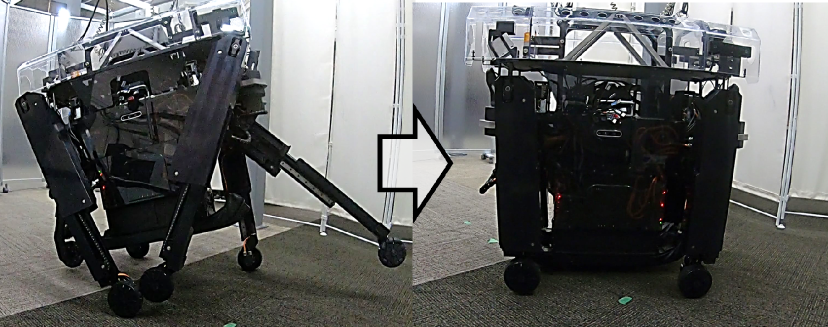
Figure 1: Standing-up motion generation task of a six-wheeled-telescopic-legged robot: Tachyon 3. The initial pose (Left) is set randomly, and the robot is requested to transition safely to the upright pose (Right).

We evaluate the effectiveness of our proposed method by applying it to the standing-up motion generation task of a six-wheeled-telescopic-legged robot: Tachyon 3 [10] (Fig. 1). To enable the robot to stand up, it is necessary to coordinate each leg, which requires more complex control than conventional quadruped robots. In addition, the task requires the robot’s controller to satisfy multiple conditions to stand up safely without damaging the hardware. We show that the task is challenging to learn with manually designed reward functions, but the proposed method succeeds in acquiring the desired behavior. Furthermore, we apply the trained policy to the robot in a real environment and demonstrate that the learned policy successfully achieves the task as it did in the simulation.

In summary, our contributions are as follows:

• Proposal of Constraints as Rewards (CaR), a new approach to train robots with reinforcement learning that enables the automatic tuning of weights among objectives by composing the task solely from constraints.

• Proposal of four specific designs of constraint function that enable an intuitive interpretation of the task objective.

• Proposal of the QRSAC-Lagrangian algorithm, which achieves fast and stable learning in reinforcement learning with CaR.

• Evaluation of the effectiveness of the proposed method in both real and simulated environments through the standing-up motion generation task of a six-wheeled-telescopic-legged robot: Tachyon 3.

II RELATED WORK

II-A Reinforcement Learning with Constraints

Constraints have been used widely in the field of reinforcement learning to restrict the training policy from deviating from the desired state. One of the main purposes of constraints is to ensure the safety of the learning policy [11]. In [8, 9], constraints are employed to define safety requirements, and the Lagrangian method is utilized to solve reinforcement learning problems with constraints. Zhang et al. converted the constraints into penalties and solved an unconstrained optimization problem to ensure safety [12]. Liu et al. [13] constrained the policy to operate in a space tangent to the unsafe region to ensure safe exploration. Constraints are also used for purposes beyond ensuring safety. Algorithms such as TRPO [14] and PPO [15] constrain the learning policy from deviation using KL-divergence as a metric. In the well-known SAC algorithm [16, 17], constraints were introduced to automatically tune the temperature parameter. Similar to our work, Elliot et al. proposed Constraints as Terminations (CaT) [4], which transform constraints into episode terminations. However, the problem formulation in previous research still focus on maximizing cumulative rewards and require manual tuning of the weights that balance different task objectives. In this paper, we propose composing tasks solely from constraints to avoid reward engineering and to automatically tune the weights among task objectives.

II-B Deep Reinforcement Learning for Legged Robots

There is no doubt that recent progress in generating complex locomotion behavior in legged robots has been achieved through deep reinforcement learning techniques. Taylor et al. [1] succeessfully retargeted human motion capture data to a small bipedal robot. Similarly, Jemin et al. [5] succeeded in making a quadruped robot stand up from a fallen pose. A quadruped robot can now perform parkour using a controller trained with reinforcement learning [3]. Furthermore, various studies have demonstrated the effectiveness of reinforcement learning [17, 4, 18, 19]. However, we assert that there may have been a significant trial-and-error process involved in reward tuning behind these successes, which is often not described in the papers. In this work, we propose a new approach to compose the task objective to mitigate this trial-and-error process. We applied the proposed approach to the standing-up motion generation task of a six-wheeled-telescopic-legged robot, Tachyon 3 [10], and demonstrated its effectiveness.

III PRELIMINARIES

In this research, we consider the finite-horizon reinforcement learning problem [20]. The objective of the problem is to find an optimal policy $\pi^{\ast}$ that maximizes the sum of discounted rewards over the horizon $T$:

$$\max_{\pi}\mathbb{E}_{\pi}[\sum_{t=0}^{T}\gamma^{t}r(s_{t},a_{t})].$$ (1)

Here, $s_{t}$, $a_{t}$, $\gamma$, and $r$ denote the state at time $t$, the action at time $t$, the discount factor, and the reward function, respectively. In this work, we revisit the design of the reward function $r(s,a)$.

As previously mentioned, in many practical applications, the reward function $r(s,a)$ is designed as a weighted sum of multiple functions $r_{n}(s,a)\ (n=1,\dots,N)$

$$r(s,a)=\sum_{n=1}^{N}w_{n}r_{n}(s,a).$$ (2)

Therefore, the actual problem that needs to be solved is:

$$\max_{\pi}\sum_{n=1}^{N}w_{n}\mathbb{E}_{\pi}\biggl{[}\sum_{t=0}^{T}\gamma^{t}r_{n}(s_{t},a_{t})\biggr{]}.$$ (3)

From this equation, we can confirm that we need to tune both weights $w_{n}$ and functions $r_{n}$ for successful learning. However, there is no systematic procedure to tune these parameters.

In this work, to alleviate the trial-and-error involved in the design of the reward function, we consider solving reinforcement learning problem with constraints. The reinforcement learning problem with constraints is defined as follows:

$$\begin{split}\max_{\pi}\ &\mathbb{E}_{\pi}\biggl{[}\sum_{t=0}^{T}\gamma^{t}r(s_{t},a_{t})\biggr{]}\\ \text{s.t.}\ &\mathbb{E}_{\pi}\biggl{[}\sum_{t=0}^{T}\gamma^{t}g_{m}(s_{t},a_{t})\biggr{]}\geq 0,\ m=1,\dots,M.\end{split}$$ (4)

Here, $g_{m}(s_{t},a_{t})$ is the $m$-th constraint function. In the next section, we will show that we can eliminate the tuning process required in the original problem using this formulation.

IV METHOD

IV-A Constraints as Rewards (CaR)

In this section, we will describe in detail the idea of Constraints as Rewards (CaR). In CaR, we transform the reinforcement learning problem with constraints described in eq. (4) into an unconstrained problem by incorporating the Lagrange dual function $L(\pi,\boldsymbol{\lambda})$ [6]:

$$\max_{\lambda_{m}>0\ \forall{m}}\max_{\pi}L(\pi,\boldsymbol{\lambda}).\\$$ (5)

Where $\boldsymbol{\lambda}=[\lambda_{1},\dots,\lambda_{M}]^{\mathsf{T}}$ are the Lagrange multipliers, and

$$\begin{split}&L(\pi,\boldsymbol{\lambda})\\ &\triangleq\mathbb{E}_{\pi}\biggl{[}\sum_{t=0}^{T}\gamma^{t}r(s_{t},a_{t})\biggr{]}+\sum_{m=1}^{M}\lambda_{m}\mathbb{E}_{\pi}\biggl{[}\sum_{t=0}^{T}\gamma^{t}g_{m}(s_{t},a_{t})\biggr{]}.\end{split}$$ (6)

The transformed problem is known as the Lagrange dual of the original problem [6]. The core idea of CaR is to set the reward function in eq. (6) to $r(s_{t},a_{t})\triangleq 0$. By doing so, we obtain the following problem to solve:

$$\max_{\lambda_{m}>0\ \forall{m}}\max_{\pi}\sum_{m=1}^{M}\lambda_{m}\mathbb{E}_{\pi}\biggl{[}\sum_{t=0}^{T}\gamma^{t}g_{m}(s_{t},a_{t})\biggr{]}.\\$$ (7)

We can see that this formulation is identical to the standard reinforcement learning problem with a reward function (eq. (3)) except for the operator $\max_{\lambda_{m}>0\ \forall{m}}$. The new formulation suggests that Lagrange multipliers, which serves as weights among constraints, can be tuned automatically. Therefore, if we design the learning objective in terms of constraints, we can obtain the desired policy without tuning the weights among different objectives.

IV-B Constraint Function Design

To compose the learning objective with constraints, we propose the following four designs of constraint function $g(s,a)$. Each design provides an intuitive interpretation for the optimization target. Timestep constraints enable constraining the robot at specific timestep (e.g., constraining the final pose of the robot.), while episode constraints enable constraining the robot during an episode (e.g., constraining the robot from hitting an obstacle.). We expect that having an intuitive interpretation will make it easier for the task designer to compose the objective. In our experiments, we composed the task objective using a combination of these functions. Please note that the inequality in each constraint can be reversed by setting the constraint function to $-g(s,a)$. See the appendix section for the derivation of each function.

1. Timestep probability constraint: Constrain the probability of an event at specific timestep $t=t^{\prime}$ to be less than or equal to $p_{\epsilon}\in[0\dots 1]$: $p_{\epsilon}\geq P_{\pi}(s_{t^{\prime}}\in\mathcal{S}^{\prime},a_{t^{\prime}}\in\mathcal{A}^{\prime})$. With:

   $$g(s,a)=\begin{cases}0\quad(t\neq t^{\prime})\\ p_{\epsilon}-\mathbf{1}_{s\in\mathcal{S}^{\prime},a\in\mathcal{A}^{\prime}}\quad(t=t^{\prime}).\end{cases}$$ (8)

2. Timestep value constraint: Constrain the value computed from a state and/or action in expectation at specific timestep $t=t^{\prime}$ to be less than or equal to $\epsilon$: $\epsilon\geq\mathbb{E}_{\pi}[\hat{g}(s_{t^{\prime}},a_{t^{\prime}})]$. With:

   $$g(s,a)=\begin{cases}0\quad(t\neq t^{\prime})\\ \epsilon-\hat{g}(s,a)\quad(t=t^{\prime}).\end{cases}$$ (9)

3. Episode probability constraint: Constrain the probability of an event during an episode to be less than or equal to $p_{\epsilon}\in[0\dots 1]$: $p_{\epsilon}\geq P_{\pi,\gamma}(s\in\mathcal{S}^{\prime},a\in\mathcal{A}^{\prime})$. With:

   $$g(s,a)=p_{\epsilon}-\mathbf{1}_{s\in\mathcal{S}^{\prime},a\in\mathcal{A}^{\prime}}.$$ (10)

4. Episode value constraint: Constrain the value computed from a state and/or action during an episode in expectation to be less than or equal to $\epsilon$: $\epsilon\geq\mathbb{E}_{\pi,\gamma}[\hat{g}(s,a)]$. With:

   $$g(s,a)=\epsilon-\hat{g}(s,a).$$ (11)

Here, $\mathcal{S}^{\prime}$ and $\mathcal{A}^{\prime}$ are the sets of events of particular interest, $\mathbf{1}$ is the indicator function, $P_{\pi}$ and $P_{\pi,\gamma}$ are the undiscounted and discounted state-action probabilities, and $\mathbb{E}_{\pi,\gamma}$ is the expectation under the discounted state-action distribution.

IV-C QRSAC-Lagrangian

We propose QRSAC-Lagrangian, an extension of QRSAC [7], to solve the reinforcement learning problem when using CaR. We extended QRSAC because we expect that the quantile function, which estimates the distribution of Q values, is effective in our problem setting. In CaR, the algorithm needs to periodically update the Lagrange multipliers. Therefore, the distribution of the target Q value changes during training. In such situations, direct estimation of Q values performed using conventional algorithms may become unstable. We will compare the performance of QRSAC-Lagrangian, when used in conjunction with CaR, with variants of Lagrangian-based algorithms, such as SAC-Lagrangian [3] and PPO-Lagrangian [8], and show that QRSAC-Lagrangian achieves faster convergence compared to these algorithms. The pseudo code of the algorithm is shown in Algorithm 1. In Algorithm 1, $\pi_{\theta}$ is the training policy, $d$ is the multiplier update interval, and $p(s_{t+1}|a_{t},s_{t})$ is the state transition distribution.

Algorithm 1 QRSAC-Lagrangian

1:Initialize policy parameters $\theta$, set replay buffer to $\mathcal{D}=\{\}$, and set Lagrange multipliers $\boldsymbol{\lambda}=\mathbf{0}$.

2:for each iteration $i$ do

3:  $a_{t}\sim\pi_{\theta}(a_{t}|s_{t})$

4:  $s_{t+1}\sim p(s_{t+1}|a_{t},s_{t})$

5:  $\mathcal{D}\leftarrow\mathcal{D}\ \cup\ \{(s_{t},a_{t},r(s_{t},a_{t}),g_{1,\dots,M}(s_{t},a_{t}),s_{t+1})\}$

6:  Update policy $\pi_{\theta}$ with QRSAC using $\mathcal{D}$ and $\boldsymbol{\lambda}$

7:  if $i\bmod d$ then

8:   for each $m$ do

9:     $\lambda_{m}\leftarrow\lambda_{m}-Adam(\alpha_{\lambda},\nabla_{\lambda_{m}}L(\pi,\boldsymbol{\lambda}))$

10:     $\lambda_{m}\leftarrow\max(\lambda_{m},0)$

11:   end for

12:  end if

13:end for

V IMPLEMENTATION

Our robot has six telescopic legs, four with driving wheels and two with omnidirectional passive wheels. Each leg has a hip joint with a range of motion of $45\text{\,}\mathrm{d}\mathrm{e}\mathrm{g}$ and a $500\text{\,}\mathrm{m}\mathrm{m}$ expandable prismatic knee joint. The policy must coordinate each leg to enable the robot to stand up during the task. In this section, we will describe the design of the constraint functions used in training and the controller design for this robot. For hardware details of the robot, please refer to [10].

V-A Constraint Function Design for Standing Up Task

We designed the following five constraints for the task:

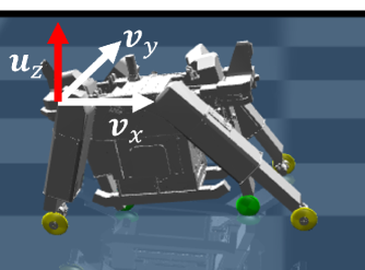
Figure 2: Relationship between $\mathbf{u}_{z}$, $\mathbf{v}_{x}$ and $\mathbf{v}_{y}$.

1. Final pose constraint:

   $$g(s,a)=\begin{cases}0\quad(t\neq T)\\ 10^{-3}-|s_{\text{target}}-s_{\text{angle/position}}|\quad(t=T).\end{cases}$$ (12)

   Existing research [5] uses an episodic reward that penalizes the robot’s pose at every timestep to facilitate standing up. However, from the perspective of constraints, the intermediate pose of the robot should be arbitrary. Therefore, we constrain the hip joint angle and knee position of the robot’s leg only at the final timestep $T$ to be below ${10}^{-3}\text{\,}\mathrm{r}\mathrm{a}\mathrm{d}$ and ${10}^{-3}\text{\,}\mathrm{m}$. $s_{\text{target}}$ is the target joint angle/knee position and $s_{\text{angle/position}}$ is the actual joint angle/knee position. We apply this constraint to each leg, resulting in a total of 12 pose constraints.

2. Fall down constraint:

   $$g(s,a)=\begin{cases}0\quad(t\neq T)\\ -\mathbf{1}_{\text{robot is in a fall-down state.}}\quad(t=T).\end{cases}$$ (13)

   This function constrains the probability of falling down to 0. The robot is considered to be in a fall-down state whenever more than five wheel joints are higher than the hip joints. The task terminates when the robot falls down: therefore, the indicator function is evaluated at $t=T$.

3. Body contact constraint:

   $$g(s,a)=-\mathbf{1}_{\text{robot's body hits the floor.}}.$$ (14)

   This function constrains the probability of the robot’s body making contact with the floor to 0.

4. Leg swing constraint:

   $$g(s,a)=-\mathbf{1}_{\text{Angular velocity exceeds 2.0 rad/s.}}$$ (15)

   This function constrains the angular velocity of the robot’s hip joint to be less than $2.0\text{\,}\mathrm{r}\mathrm{a}\mathrm{d}\mathrm{/}\mathrm{s}$, preventing dangerous leg swinging actions. To evaluate this constraint, we terminated the episode whenever the joint’s angular velocity exceeds $2.0\text{\,}\mathrm{r}\mathrm{a}\mathrm{d}\mathrm{/}\mathrm{s}$.

5. Inclination constraint:

   $$g(s,a)=\begin{cases}0\quad(t\neq T)\\ 10^{-2}-|\mathbf{u}_{z}^{\mathsf{T}}\mathbf{v}_{x,y}|\quad(t=T).\end{cases}$$ (16)

   We add this constraint to ensure that the final pose of the robot remains parallel to the floor. We constrain the robot’s body to be perpendicular to the z-axis. Here, $\mathbf{u}_{z}=[0,0,1]^{\mathsf{T}}$ is the unit vector along the z-axis, and $\mathbf{v}_{x}$ and $\mathbf{v}_{y}$ are the normalized vectors connecting the leg joints (Fig. 2).

V-B Robot Controller Design

TABLE I: Network structure of $\pi_{\theta}$

Input layer	state input
Middle layer 1	Fully-connected followed by ReLU (256 dim)
Middle layer 2	Fully-connected followed by ReLU (256 dim)
Middle layer 3	Fully-connected followed by ReLU (256 dim)
Output layer	Gaussian mean (12 dim) and variance (12 dim)

Our robot is controlled with a PID controller that receives the target joint angles and positions of each leg. Therefore, we trained a controller $\pi_{\theta}$ that outputs the target joint angles and positions to be input to this PID-controller. Table I shows its network architecture. The policy inputs a vector consisting of the following features:

• Hip joint angles (6 dim)

• Knee joint positions (6 dim)

• Hip joint angular velocities (6 dim)

• Knee joint velocities (6 dim)

• Robot’s angular velocities and accelarations (6 dim)

• Timestep since the beginning of the task (1 dim)

• History of policy’s output (12 dim$\times H$ steps).

The output of the policy is squashed and normalized using the tanh function to fit within the range of $[-1,1]$. Therefore, we rescaled the policy’s output before feeding it to the PID-controller. We fixed the robot’s wheel velocity to 0 for the standing-up task. We set $H=3$ in the simulation and $H=5$ in the real robot experiment.

VI EXPERIMENTS

VI-A Experimental Setup

TABLE II: Reward functions for comparison. $\boldsymbol{p}_{t}$ denotes a vector at time $t$ that consists of joint angles, joint angular velocities, knee positions, and knee velocities of each leg. The target value of $\boldsymbol{p}$ at upright pose is $\boldsymbol{p}=\bf{0}$.

Reward design 1
Pose reward	$\begin{cases}1/(||\boldsymbol{p}_{t}||+1)\quad(t=T)\\ 0\quad(t\neq T)\end{cases}$
Fall down penalty	-1
Reward design 2
Pose penalty	$-w\times||\boldsymbol{p}_{t}||\quad(w=0.001)$
Fall down penalty	-1
Reward design 3
Pose reward	$\begin{cases}1/(||\boldsymbol{p}_{t}||+1)\quad(t=T)\\ 1/(||\boldsymbol{p}_{t}||+1)-1/(||\boldsymbol{p}_{t-1}||+1)\quad(t\neq T)\end{cases}$
Fall down penalty	-1
Reward design 4
Pose reward	$1/(||\boldsymbol{p}_{t}||+1)$
Fall down penalty	-1
Reward design 5
Pose reward	$\exp(-||\boldsymbol{p}_{t}||)$
Fall down penalty	-1

In the experiment, we trained the policy to make the robot transition from an arbitrary initial pose to an upright pose (See Fig. 1) and tested its performance using 10 different initial poses. We built a simulation environment using MuJoCo [21] and trained the policy for 1 million iterations. To facilitate faster convergence, we performed curriculum training, starting from an initial pose near the upright position and gradually increasing the distance from the upright pose. We did not perform parallel simulations to train the policy and used only one simulated robot to collect data during training. In all experiments, the trained controller operates at $10\text{\,}\mathrm{H}\mathrm{z}$. See the appendix for the hyperparameters used in the experiment.

In the simulation, we evaluated the proposed method comparing it with:

• A policy learned using manually designed reward functions: Table II shows the five different reward functions designed based on the task’s learnability.

• A policy learned using conventional methods: We compared the proposed QRSAC-Lagrangian with conventional algorithms such as SAC-Lagrangian [9], PPO-Lagrangian [8], and CaT [4].

Additionally, we assessed the robustness of the policy by testing it on terrains different from the trained environment. Furthermore, we conducted an ablation study to evaluate the efficacy of each constraint designed in the previous section.

For the real robot experiment, we ran the policy trained with the proposed method without any fine-tuning on real data and evaluated its performance.

VI-B Evaluation Results

	(0.679)	(0.477)	(0.750)	(0.670)	(0.640)	(0.930)
	(0.420)	(0.476)	(0.751)	(0.671)	(0.458)	(0.930)
	Design 1	Design 2	Design 3	Design 4	Design 5	CaR (ours)
Initial pose	Final pose (The number in parenthesis is the final pose score.)

Figure 3: Final poses of the robot. Leftmost figure shows the initial pose of each row. The policy trained with manually designed rewards fails to transition to the upright pose. In contrast, our proposed method (CaR) succeeds in standing up.

Fig. 3 shows the final pose of the robot when running policies trained with manually designed rewards and the proposed method. The pose score $1/(||\boldsymbol{p}_{t}||+1)$ is also shown in parenthesis. From the figure, we can confirm that CaR succeeds in transitioning to the target pose. In contrast, policies trained with manually designed rewards fail to transition to the target pose. Among the policies trained with manually designed rewards, Design 3 exhibits the highest final pose score; however, this score remains lower compared to the proposed method. We do not claim that there is no reward function that can achieve this task. However, from the experiment, we can confirm that designing a reward function is not a straightforward task, and the proposed method is effective even in such situations.

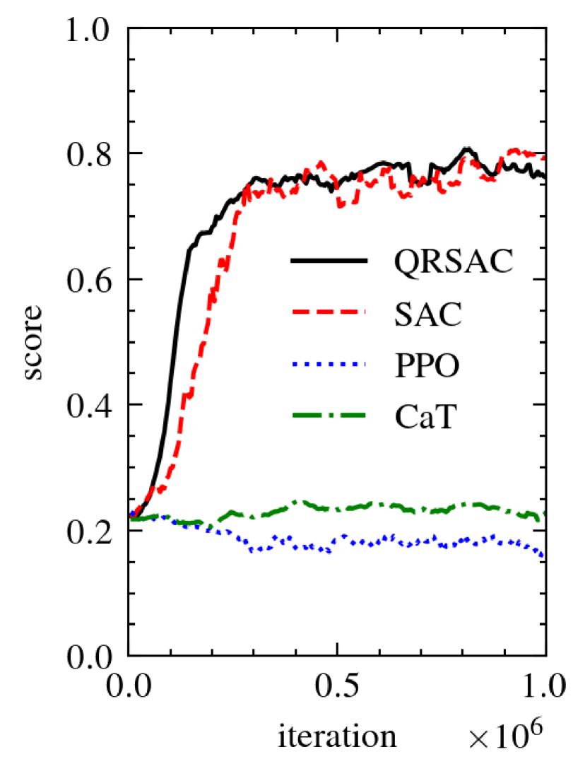
(a) Algorithm learning curve.

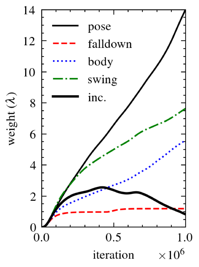
(b) Weight parameters.

Figure 4: Algorithm learning curve and tuning history of weight parameters. The learning curve shows the average of 5 runs initialized with different random seeds. The weight of the pose parameter shown on the right is the weight of the left-front hip joint (Other weight parameters for pose constraints also exhibited similar changes).

Fig. 4 shows the learning curve of the proposed algorithm and comparison algorithms in the task. From the figure, we can confirm that the proposed QRSAC-Lagrangian achieves faster and more robust convergence compared to conventional algorithms. PPO-Lagrangian and CaT failed to learn the task. SAC-Lagrangian achieves similar final performance, but its convergence is slower compared to QRSAC-Lagrangian. The difference between SAC-Lagrangian and QRSAC-Lagrangian lies solely in the underlying reinforcement learning algorithm. This result suggest that the quantile function introduced in QRSAC is effective in the setting of CaR, where the distrubution of the target Q value dynamically changes during training. Also, refer to the appendix for results confirming similar findings in the classic inverted pendulum task. Fig. 4 shows the tuning results of weight parameters conducted by the proposed algorithm. We can confirm that weight parameters were tuned dynamically during training. The weight for fall-down constraint converged quickly because the robot learned to avoid falling down at the beginning of training. In contrast, the weights for the pose constraint, body constraint, and swing constraint gradually incresed during the course of training. This result indicates that these constraints were challenging for the policy to meet. The weight for inclination constraint increased from the beginning to the middle of training but decreased towards the end. This is because the policy succeeded in keeping the final pose parallel to the floor by the middle of training, and the algorithm decreased its weight towards the end to prioritize the pose, body, and swing constraints more.

(0.902)	(0.902)	(0.903)
Flat	Rough	Slope

Figure 5: Policy execution results on different types of terrain. (Top) Initial pose. (Bottom) Final pose. Policy is only trained in a flat terrain environment but works on different types of terrain. The score in parenthesis is the final pose score.

Fig. 5 shows the execution results of the trained policy in three different environments. The flat terrain environment is the trained environment. The rough terrain environment has a random height of up to $0.05\text{\,}\mathrm{m}$. The slope terrain environment has a slope of $10\text{\,}\mathrm{d}\mathrm{e}\mathrm{g}$. From the figure, we can confirm the robustness of the policy. The trained policy succeeds in completing the task even in environments different from the original trained environment.

TABLE III: Ablation results. Each value is the average of 10 runs. Contact is the ratio of robot’s body making contact with the floor during the task. Max $\omega_{\text{joint}}$ is the maximum angular velocity of the leg joint recorded during the task. $\theta_{T,\text{roll}}$ and $\theta_{T,\text{pitch}}$ are the roll and pitch angles of the robot at the final timestep. $\uparrow$ and $\downarrow$ indicate that a higher value is better and a lower value is better, respectively. (P: Pose constraint, F: Fall-down constraint, C: Contact constraint, S: Swing constraint, I: Inclination constraint)

	Pose	Contact	Max $\omega_{\text{joint}}$	$\theta_{T}^{\text{roll}}$	$\theta_{T}^{\text{pitch}}$
	score $\uparrow$	[%] $\downarrow$	[rad/s] $\downarrow$	[deg] $\downarrow$	[deg] $\downarrow$
P+F	0.925	0.5	3.038	3.896	5.672
P+F+C	0.920	0.1	8.937	6.933	3.782
P+F+C+S	0.901	1.0	1.136	3.839	4.698
P+F+C+S+I	0.896	0.6	1.673	0.057	0.057

Table III shows the results of the ablation study on the designed constraint functions. From the table, we can confirm that each constraint succeeded in improving the performance of the corresponding metric. Additionally, while it is challenging to perfectly satisfy each constraint, the average performance of the policy trained with all five constraints appears reasonable. Based on these results, we used the policy trained with all five constraints in the real robot experiment.

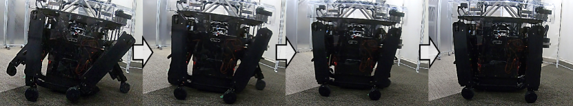
Figure 6: Policy execution result on the real robot. (Top) Pose used in simulation. (Bottom) Challenging pose with expanded knees.

Fig. 6 shows the execution result of the trained policy in a real environment. From the figure, we can confirm that the policy succeeds in completing the task on the real robot. We tested 10 poses used in the simulation and 9 challenging poses with expanded knees, and confirmed that the policy successfully transitions to the upright pose from all poses.

VII CONCLUSION AND FUTURE WORK

In this paper, we introduced the concept of Constraints as Rewards (CaR) to mitigate the extensive trial-and-error involved in tuning a reward function. Instead of designing a reward function, CaR composes the task objective solely from constraint functions. In this approach, unlike conventional reward function design, we do not need to manually tune the weights among task objectives; the weights are adjusted automatically during the training process. In addition, to simplify the design of constraint functions, we proposed four specific designs that provide an intuitive interpretation of the task objective. Furthermore, we introduced QRSAC-Lagrangian algorithm to solve this reinforcement learning problem with constraints. We demonstrated the effectiveness of our method by applying it to the standing-up motion generation task of a six-wheeled-telescopic-legged robot, Tachyon 3. While this task is challenging to learn with manually designed reward functions, our proposed method enabled the robot to effectively learn the target behavior.

We believe that CaR is effective for a wide range of robotic tasks. However, CaR requires the task to be expressed solely in terms of constraint functions. Therefore, it might be challenging to apply in tasks where pure maximization is required (e.g., make the robot walk as fast as possible). In such cases, it would be beneficial to combine reward functions with constraint functions. Exploring an effective objective design method for such tasks could be a promising direction for future work.

Appendix A Constraint function derivation

In the derivation, we assume discrete state and action sets but the results can also be applied to continuous settings.

A-A Derivation of timestep probability constraint

By substituting eq. (5) into the optimization objective, we get:

$$\mathbb{E}_{\pi}[\sum_{t=0}^{T}\gamma^{t}g(s_{t},a_{t})]$$

$$= \mathbb{E}_{\pi}[\gamma^{t^{\prime}}(p_{\epsilon}-\mathbf{1}_{s\in\mathcal{S}^{\prime},a\in\mathcal{A}^{\prime}})]\quad(\because\ g(s_{t},a_{t})=0\ t\neq t^{\prime})$$

$$= \gamma^{t^{\prime}}(p_{\epsilon}-\mathbb{E}_{\pi}[\mathbf{1}_{s\in\mathcal{S}^{\prime},a\in\mathcal{A}^{\prime}}])$$

$$= \gamma^{t^{\prime}}(p_{\epsilon}-P_{\pi}(s\in\mathcal{S}^{\prime},a\in\mathcal{A}^{\prime})).$$

Therefore, the constraint can be expressed as follows:

$$\gamma^{t^{\prime}}(p_{\epsilon}-P_{\pi}(s\in\mathcal{S}^{\prime},a\in\mathcal{A}^{\prime}))\geq 0\rightarrow p_{\epsilon}\geq P_{\pi}(s\in\mathcal{S}^{\prime},a\in\mathcal{A}^{\prime}).$$

A-B Derivation of timestep value constraint

Similar to the above derivation, by substituting eq.6 into the optimization objective, we get:

$$\gamma^{t^{\prime}}(\epsilon-\mathbb{E}_{\pi}[\hat{g}(s_{t^{\prime}},a_{t^{\prime}})])\geq 0\rightarrow\epsilon\geq\mathbb{E}_{\pi}[\hat{g}(s_{t^{\prime}},a_{t^{\prime}})].$$

A-C Derivation of episode probability constraint

First, we reformulate the optimization objective as follows:

$$\mathbb{E}_{\pi}[\sum_{t=0}^{T}\gamma^{t}g(s_{t},a_{t})]$$

$$= \sum_{t=0}^{T}\sum_{s_{0}\in\mathcal{S},\dots,a_{T}\in\mathcal{A}}p(s_{0},a_{0},\dots,s_{T},a_{T})\gamma^{t}g(s_{t},a_{t})$$

$$= \sum_{t=0}^{T}\sum_{s\in\mathcal{S}}\sum_{a\in\mathcal{A}}p_{t}^{\pi}(s,a)\gamma^{t}g(s,a)$$

$$= \sum_{s\in\mathcal{S}}\sum_{a\in\mathcal{A}}g(s,a)\sum_{t=0}^{T}p^{\pi}_{t}(s,a)\gamma^{t}$$

$$= \frac{1-\gamma^{T+1}}{1-\gamma}\sum_{s\in\mathcal{S}}\sum_{a\in\mathcal{A}}g(s,a)\sum_{t=0}^{T}p^{\pi}_{t}(s,a)\frac{1-\gamma}{1-\gamma^{T+1}}\gamma^{t}.$$

Here, $p^{\pi}_{t}(s,a)$ is the state-action probability distribution at time $t$ under policy $\pi$. By defining the discounted state-action distribution as:

$$p_{\pi,\gamma}(s,a)\triangleq\sum_{t=0}^{T}p^{\pi}_{t}(s,a)\frac{1-\gamma}{1-\gamma^{T+1}}\gamma^{t},$$

the original expectation can be rewritten as:

$$\mathbb{E}_{\pi}\biggr{[}\sum_{t=0}^{T}\gamma^{t}g(s_{t},a_{t})\biggl{]}\propto\mathbb{E}_{(s,a)\sim p_{\pi,\gamma}}\biggr{[}g(s,a)\biggl{]}$$

Next, by substituting eq. (7), we get:

$$\mathbb{E}_{\pi}[\sum_{t=0}^{T}\gamma^{t}g(s_{t},a_{t})] \propto\mathbb{E}_{(s,a)\sim p_{\pi,\gamma}}\biggr{[}g(s,a)\biggl{]}$$

$$=\mathbb{E}_{(s,a)\sim p_{\pi,\gamma}}\biggr{[}(p_{\epsilon}-\mathbf{1}_{s\in\mathcal{S}^{\prime},a\in\mathcal{A}^{\prime}})\biggl{]}$$

$$=(p_{\epsilon}-\mathbb{E}_{(s,a)\sim p_{\pi,\gamma}}\biggr{[}\mathbf{1}_{s\in\mathcal{S}^{\prime},a\in\mathcal{A}^{\prime}}\biggl{]})$$

$$=p_{\epsilon}-P_{\pi,\gamma}(s\in\mathcal{S}^{\prime},a\in\mathcal{A}^{\prime}).$$

Therefore, the constraint can be expressed as follows:

$$p_{\epsilon}-P_{\pi,\gamma}(s\in\mathcal{S}^{\prime},a\in\mathcal{A}^{\prime})\geq 0.\rightarrow p_{\epsilon}\geq P_{\pi,\gamma}(s\in\mathcal{S}^{\prime},a\in\mathcal{A}^{\prime}).$$

A-D Derivation of episode value constraint

Similar to the above derivation, by sustituting eq. (8) into the optimization objective, we get:

$$\frac{1-\gamma^{T+1}}{1-\gamma}(\epsilon-\mathbb{E}_{\pi,\gamma}[\hat{g}(s,a)])\geq 0\rightarrow\epsilon\geq\mathbb{E}_{\pi,\gamma}[\hat{g}(s,a)].$$

Here, $\mathbb{E}_{\pi,\gamma}$ is the expectation under the discounted state-action distribution $p_{\pi,\gamma}$.

Appendix B Hyperparameters and experimental settings

TABLE IV: QRSAC-Lagrangian hyperparameters

Adam parameters	$\beta_{1}=0.9$, $\beta_{2}=0.999$
Model learning rate	$3.0\times 10^{{}^{-}4}$
Multiplier learning rate ($\alpha_{\lambda}$)	0.1
Multiplier update interval ($d$)	5000
Discount factor $\gamma$	0.99
Batch size	256
Quantile points	32
Network update coefficient $\tau$	0.005

TABLE V: Network structure of quantile function

Input layer	state and action input
Middle layer 1	Fully-connected followed by relu (256 dim)
Middle layer 2	Fully-connected followed by relu (256 dim)
Middle layer 3	Fully-connected followed by relu (256 dim)
Output layer	Quantile values (32 dim)

TABLE VI: Noise applied to model input during training. $\mathcal{N}(\mu,\sigma^{2})$ is a Gaussian distribution with mean $\mu$ and variance $\sigma^{2}$.

Joint angle noise	$\mathcal{N}(\mu=0,\sigma^{2}=0.005)$
Knee position noise	$\mathcal{N}(\mu=0,\sigma^{2}=0.005)$
Joint angular velocity noise	$\mathcal{N}(\mu=0,\sigma^{2}=0.01)$
Knee velocity noise	$\mathcal{N}(\mu=0,\sigma^{2}=0.01)$
Robot’s angular velocity noise	$\mathcal{N}(\mu=0,\sigma^{2}=0.01)$
Robot’s accelaration noise	$\mathcal{N}(\mu=0,\sigma^{2}=0.1)$
Timestep noise	$\mathcal{N}(\mu=0,\sigma^{2}=0.1)$

Hyperparameters and settings used in the experiments are listed in Table IV,Table V, and Table VI.

Appendix C Extra experimental results

We present the evaluation results of the proposed algorithm in the classic inverted pendulum task implemented in Gym [22]. We trained the model using two different constraint functions:

$$g(s,a)=10^{-2}-|\theta_{p}|$$ (17)

and

$$g(s,a)=\begin{cases}0\quad(t\neq T)\\ 10^{-2}-|\theta_{p}|\quad(t=T).\end{cases}$$ (18)

Here, $\theta_{p}$ is the angle of the pendulum.

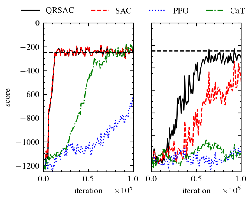
Figure 7: Learning curve of each algorithm trained with eq. (17) (Left) and eq. (18) (Right). Dotted line is the score when trained with original reward function.

Fig. 7 shows the learning curves during training. From the figure, we can confirm that conventional PPO-Lagrangian and CaT failed to learn with the constraint function in eq. (18). This result suggests that PPO-Lagrangian and CaT are not effective in environments with constraint functions of the form in eq. (18). Conversely, SAC-Lagrangian and QRSAC-Lagrangian succeeded in learning in both settings. As in the experiment section, QRSAC-Lagrangian converged faster than SAC-Lagrangian.

References

- [1] M. Taylor, S. Bashkirov, J. F. Rico, I. Toriyama, N. Miyada, H. Yanagisawa, and K. Ishizuka, “Learning bipedal robot locomotion from human movement,” in 2021 IEEE International Conference on Robotics and Automation (ICRA), 2021, pp. 2797–2803.
- [2] E. Kaufmann, L. Bauersfeld, A. Loquercio, M. Müller, V. Koltun, and D. Scaramuzza, “Champion-level drone racing using deep reinforcement learning,” Nature, vol. 620, no. 7976, pp. 982–987, 2023.
- [3] Z. Zhuang, Z. Fu, J. Wang, C. Atkeson, S. Schwertfeger, C. Finn, and H. Zhao, “Robot parkour learning,” in Conference on Robot Learning (CoRL), 2023.
- [4] E. Chane-Sane, P.-A. Leziart, T. Flayols, O. Stasse, P. Souères, and N. Mansard, “Cat: Constraints as terminations for legged locomotion reinforcement learning,” in IEEE/RSJ International Conference on Intelligent Robots and Systems (IROS), 2024.
- [5] J. Hwangbo, J. Lee, A. Dosovitskiy, D. Bellicoso, V. Tsounis, V. Koltun, and M. Hutter, “Learning agile and dynamic motor skills for legged robots,” Science Robotics, vol. 4, no. 26, 2019.
- [6] S. Boyd and L. Vandenberghe, Convex optimization. Cambridge university press, 2004.
- [7] P. Wurman, S. Barrett, K. Kawamoto, J. MacGlashan, K. Subramanian, T. Walsh, R. Capobianco, A. Devlic, F. Eckert, F. Fuchs, L. Gilpin, P. Khandelwal, V. Kompella, H. Lin, P. MacAlpine, D. Oller, T. Seno, C. Sherstan, M. Thomure, and H. Kitano, “Outracing champion gran turismo drivers with deep reinforcement learning,” Nature, vol. 602, pp. 223–228, 02 2022.
- [8] J. Achiam and D. Amodei, “Benchmarking safe exploration in deep reinforcement learning,” 2019. [Online]. Available: https://api.semanticscholar.org/CorpusID:208283920
- [9] S. Ha, P. Xu, Z. Tan, S. Levine, and J. Tan, “Learning to walk in the real world with minimal human effort,” in Proceedings of the 2020 Conference on Robot Learning, ser. Proceedings of Machine Learning Research, J. Kober, F. Ramos, and C. Tomlin, Eds., vol. 155. PMLR, 16–18 Nov 2021, pp. 1110–1120.
- [10] N. Takasugi, M. Kinoshita, Y. Kamikawa, R. Tsuzaki, A. Sakamoto, T. Kai, and Y. Kawanami, “Real-time perceptive motion control using control barrier functions with analytical smoothing for six-wheeled-telescopic-legged robot tachyon 3,” in IROS. IEEE, 2024.
- [11] J. García, Fern, and o Fernández, “A comprehensive survey on safe reinforcement learning,” Journal of Machine Learning Research, vol. 16, no. 42, pp. 1437–1480, 2015.
- [12] L. Zhang, L. Shen, L. Yang, S. Chen, X. Wang, B. Yuan, and D. Tao, “Penalized proximal policy optimization for safe reinforcement learning,” 07 2022, pp. 3719–3725.
- [13] P. Liu, D. Tateo, H. B. Ammar, and J. Peters, “Robot reinforcement learning on the constraint manifold,” in Proceedings of the 5th Conference on Robot Learning, ser. Proceedings of Machine Learning Research, A. Faust, D. Hsu, and G. Neumann, Eds., vol. 164, 2022, pp. 1357–1366.
- [14] J. Schulman, S. Levine, P. Abbeel, M. Jordan, and P. Moritz, “Trust region policy optimization,” in Proceedings of the 32nd International Conference on Machine Learning, ser. Proceedings of Machine Learning Research, F. Bach and D. Blei, Eds., vol. 37. Lille, France: PMLR, 07–09 Jul 2015, pp. 1889–1897.
- [15] J. Schulman, F. Wolski, P. Dhariwal, A. Radford, and O. Klimov, “Proximal policy optimization algorithms,” CoRR, vol. abs/1707.06347, 2017. [Online]. Available: http://arxiv.org/abs/1707.06347
- [16] T. Haarnoja, A. Zhou, P. Abbeel, and S. Levine, “Soft actor-critic: Off-policy maximum entropy deep reinforcement learning with a stochastic actor,” in Proceedings of the 35th International Conference on Machine Learning, ser. Proceedings of Machine Learning Research, J. Dy and A. Krause, Eds., vol. 80. PMLR, 10–15 Jul 2018, pp. 1861–1870.
- [17] T. Haarnoja, A. Zhou, K. Hartikainen, G. Tucker, S. Ha, J. Tan, V. Kumar, H. Zhu, A. Gupta, P. Abbeel, and S. Levine, “Soft actor-critic algorithms and applications,” 2019. [Online]. Available: https://arxiv.org/abs/1812.05905
- [18] J. Lee, L. Schroth, V. Klemm, M. Bjelonic, A. Reske, and M. Hutter, “Evaluation of constrained reinforcement learning algorithms for legged locomotion,” CoRR, vol. abs/2309.15430, 2023. [Online]. Available: https://doi.org/10.48550/arXiv.2309.15430
- [19] T. Haarnoja, B. Moran, G. Lever, S. H. Huang, D. Tirumala, J. Humplik, M. Wulfmeier, S. Tunyasuvunakool, N. Y. Siegel, R. Hafner, M. Bloesch, K. Hartikainen, A. Byravan, L. Hasenclever, Y. Tassa, F. Sadeghi, N. Batchelor, F. Casarini, S. Saliceti, C. Game, N. Sreendra, K. Patel, M. Gwira, A. Huber, N. Hurley, F. Nori, R. Hadsell, and N. Heess, “Learning agile soccer skills for a bipedal robot with deep reinforcement learning,” Science Robotics, vol. 9, no. 89, 2024.
- [20] R. S. Sutton and A. G. Barto, Reinforcement Learning: An Introduction, 2nd ed. The MIT Press, 2018.
- [21] E. Todorov, T. Erez, and Y. Tassa, “Mujoco: A physics engine for model-based control.” in IROS. IEEE, 2012.
- [22] G. Brockman, V. Cheung, L. Pettersson, J. Schneider, J. Schulman, J. Tang, and W. Zaremba, “Openai gym,” 2016. [Online]. Available: arXiv:1606.01540