Optimal qubit-mediated quantum heat transfer via non-commuting operators and strong coupling effects

Abstract

Heat transfer in quantum systems is a current topic of interest due to emerging quantum technologies that attempt to miniaturize engines and examine fundamental aspects of thermodynamics. In this work, we consider heat transfer between two thermal reservoirs in which a central spin degree of freedom mediates the process. Our objective is to identify the system-bath coupling operators that maximize heat transfer at arbitrary system-bath coupling strengths. By employing a Markovian embedding method in the form of the reaction-coordinate mapping, we study numerically heat transfer at arbitrary system-bath coupling energy and for general system-bath coupling operators between the baths and the central qubit system. We find a stark contrast in the conditions required for optimal heat transfer depending on whether the system is weakly or strongly coupled to the heat baths. In the weak-coupling regime, optimal heat transfer requires identical coupling operators that facilitate maximum sequential transport, resonant with the central qubit. In contrast, in the strong-coupling regime, non-commuting system-bath coupling operators between the hot and cold reservoirs are necessary to achieve optimal heat transfer. We further employ the Effective Hamiltonian theory and gain partial analytical insights on the observed phenomena. We discuss the limitations of this approximate method in capturing the behavior of the heat current for non-commuting coupling operators, calling for its future extensions to capture transport properties in systems with general interaction Hamiltonians.

I Introduction

State-of-the-art technologies operating at the nanoscale attempt to employ exciting phenomena, such as the harnessing of quantum resources Goold et al. (2016), to manipulate energy transfer in quantum thermal machines Kosloff and Levy (2014); Benenti et al. (2017); Mitchison (2019). Conversely, thermal machines can be used to generate and manipulate quantum states Khandelwal et al. (2020); Tavakoli et al. (2020). In such configurations, one typically considers multiple thermal reservoirs held at different temperatures coupled to a central quantum system operating autonomously as a working medium. Beyond fundamental aspects at the level of our understanding of the thermodynamics, quantum thermal machines are experimentally realized in different platforms. In trapped-ion experiments Rossnagel et al. (2016); Maslennikov et al. (2019); von Lindenfels et al. (2019); Van Horne et al. (2020) the degree of control allows for single-atom working media. Nano-mechanical engines showed efficiencies beyond the standard Carnot limit—when coupled to squeezed thermal noise  Klaers et al. (2017). Nitrogen vacancy centers in diamond Maze et al. (2008); Bar-Gill et al. (2012) also allow experimental testbeds for quantum thermal machines, in which quantum coherence plays a central role in thermal efficiency Klatzow et al. (2019). More recently, demonstrations with noisy intermediate quantum computers allowed for a higher degree of control with respect to the working media in quantum thermal machines and their interactions with the bath Chen et al. (2024). Simulating true thermal reservoirs still appears to be a challenge in such platforms, although progress has been made in this direction with current hardware Motta et al. (2020). Interestingly, superconducting qubits Ronzani et al. (2018); Senior et al. (2020); Upadhyay et al. (2024) and molecular junctions Tan et al. (2011) also provide a platform for quantum heat engines with a focus on strong coupling effects. For example, in molecular junctions, the interactions between the molecule and the metal electrodes dictate the strength of the system-bath coupling. By controlling the chemical bonds at the contacts, it becomes possible to engineer strongly-coupled system-bath setups.

Fundamentally, a particular limit of interest is whenever the interaction energy of the coupling between the system and the baths is a small energy scale with respect to the system’s energy scale and temperature, and the internal dynamics of the baths is fast relative to the system’s characteristic relaxation timescale. In this case, the usual Born-Markov approximation ubiquitous in open systems theory Breuer and Petruccione (2007) is justified. Assuming the system is coupled to two baths kept at different temperatures, in the limit of long times, the system reaches a non-equilibrium steady state (NESS). For central single-spin systems and bosonic reservoirs, it follows that in this weak coupling Markovian limit, the energy current in the NESS behaves as $j_{\rm NESS}\propto\lambda^{2}$, where $\lambda$ is a parameter that dictates the energy scale of the system-bath coupling configuration Segal and Nitzan (2005); Segal (2006). Furthermore, in this limit, the heat exchange processes are fully resonant, with energy quanta transferred between the baths in resonance with the central spin frequency. With respect to the central system, the consensus is that for single-atomic/qubit systems, it is required that the baths induce maximal sequential transport within the system such that optimal energy transfer can be achieved through these transitions Kosloff (2013); Kosloff and Levy (2014). If the working medium, instead, corresponds to a many-body system; the transport properties of the entire system-bath configuration will typically depend on the microscopic details of the model. Heat transport may be coherent (ballistic) or incoherent (diffusive or anomalous) depending on the relevance of non-linear interactions among each constituent of the many-body system Lepri et al. (2003); Dhar (2008); Chen et al. (2014); Brenes et al. (2020); Barra (2015); Žnidarič (2010, 2011).

As the system-bath coupling parameter $\lambda$ is increased, the heat current increases due to the enhancement of the excitation/relaxation processes—until it turns over and becomes suppressed at higher values of $\lambda$. This behavior, and other strong-coupling aspects of heat transport, have been demonstrated by developing and implementing a plethora of analytical and numerical techniques, including wavefunction based simulations Velizhanin et al. (2008), path integral methods Kilgour et al. (2019); Chen (2023), Majorana fermion representations Agarwalla and Segal (2017), tensor network representations Brenes et al. (2020); Popovic et al. (2021), Markovian embeddings Anto-Sztrikacs and Segal (2021); Ivander et al. (2022), hierarchical equations of motion Kato and Tanimura (2016, 2018); Xu et al. (2021); Pleasance and Petruccione (2024), approximate analytical techniques Nicolin and Segal (2011); Segal (2014), mixed quantum-classical approaches Liu et al. (2018); Carpio-Martínez and Hanna (2021); Kelly (2019), quantum master equations Wang et al. (2015, 2017); Magazzù et al. (2024), variational polaron transformations Xu and Cao (2016); Hsieh et al. (2019) and the Effective Hamiltonian method Anto-Sztrikacs et al. (2023a, b). At strong coupling, non-Markovian effects may be prominent, which hinder the applicability of Markovian theories.

The scenario typically studied in the references mentioned before considers system-bath coupling operators that do not commute with the central system Hamiltonian. This condition is required for heat transfer Kosloff (2013); Kosloff and Levy (2014). However, in most studies of quantum transport through impurities, the operators of the system that couple to the baths are equivalent for the cold ($\hat{S}^{C}$) and hot ($\hat{S}^{H}$) baths, such that (trivially) these operators commute with each other, $[\hat{S}^{C},\hat{S}^{H}]=0$. A less explored direction corresponds to the case whenever $[\hat{S}^{C},\hat{S}^{H}]\neq 0$, and particularly at a strong system-bath coupling energy. Previous studies have explored scenarios where the system-bath coupling operators are non-commuting Duan et al. (2020); Anto-Sztrikacs et al. (2022); Zhang et al. (2024), focusing on specific choices of $\hat{S}^{C}$ and $\hat{S}^{H}$. However, these works did not address the general configuration needed to determine the conditions for optimal heat transfer.

In this work, we consider quantum heat transfer across a junction in which the central system is composed of a single spin degree of freedom. We select a general class of system-baths coupling operators including cases in which $[\hat{S}^{C},\hat{S}^{H}]\neq 0$, in order to investigate if different system-baths coupling operators have an effect on heat transfer at arbitrary system-baths coupling energy. Beyond the weak system-bath coupling energy limit, evaluating heat currents is usually a complicated task as non-resonant and non-Markovian effects may be prominent. To study the heat current at an arbitrary coupling energy, we consider a Markovian embedding method Woods et al. (2014) known as the reaction coordinate mapping Iles-Smith et al. (2014); Strasberg et al. (2016); Anto-Sztrikacs and Segal (2021); Hughes et al. (2009a, b). This numerical approach has been shown to lead to correct behavior at arbitrary system-baths coupling energy, when tested for a specific model of the baths spectral function Iles-Smith et al. (2014); Strasberg et al. (2016); Anto-Sztrikacs and Segal (2021).

We observe a striking contrast in the behavior of the heat current depending on the energy scale of the system-bath coupling. At weak coupling, optimal heat transfer occurs when the system-bath coupling operators maximize sequential-resonant transport utilizing the energy transitions of the spin, achieved when the system is coupled to the two baths through specific identical operators. However, at arbitrary coupling strength, this is no longer the case. In fact, the coupling operators $\hat{S}$ that optimize heat transfer in weak couplings lead to insulating behavior in strong coupling. To maximize the heat current in the strong coupling regime, different coupling operators are required for hot and cold baths, satisfying $[\hat{S}^{C},\hat{S}^{H}]\neq 0$. To address this behavior, we employ the recently developed Effective Hamiltonian theory for non-commuting system-bath coupling operators Garwoła and Segal (2024). Through the dressing of operators, the method reveals the symmetry of specific configurations that promote optimal transport at strong coupling. As for the heat current, while the Effective method performs well for commuting operators, even in the strong-coupling regime, it fails to predict the correct behavior of the steady state heat current when $[\hat{S}^{C},\hat{S}^{H}]\neq 0$. To understand this limitation, we present an analysis based on the eigenvalues of the relevant polaron-transformed system Hamiltonian.

The rest of this article is organized as follows. Sec. II provides the fundamental description of the heat currents in the NESS for a generic open quantum system. It also includes a description of our numerical methodology to study strong-coupling thermodynamics, and results of simulations at weak and arbitrary strong system-baths coupling energies. Sec III is devoted to the analytical Effective Hamiltonian theory for non-commuting system-bath coupling operators. We introduce the method and explain its predictions and limitations. We conclude with final remarks and future aspects in Sec. IV.

II Heat transport with non-commuting coupling operators

We consider the out-of-equilibrium dynamics of a quantum system $S$ coupled to two bosonic baths, each of which contains an infinite number of bosonic degrees of freedom. The total Hamiltonian is described by ($\hbar=1$)

$$\hat{H}=\hat{H}_{S} +\hat{H}_{I}+\hat{H}_{B}$$

$$=\hat{H}_{S} +\sum_{\alpha=L,R}\hat{S}^{\alpha}\sum_{k}t_{k,\alpha}\left(\hat{c}_{k,\alpha}^{\dagger}+\hat{c}_{k,\alpha}\right)$$

$$+\sum_{\alpha=L,R}\sum_{k}\nu_{k,\alpha}\hat{c}_{k,\alpha}^{\dagger}\hat{c}_{k,\alpha}.$$ (1)

We denote by $\alpha=L,R$ the left and right baths, respectively. Furthermore; $\hat{H}_{S}$ is the system Hamiltonian, the set $\{\hat{c}_{k,n}\}$ are bosonic destruction operators for the $\alpha$-th bath, while $\nu_{k,\alpha}$ and $t_{k,\alpha}$ are the frequencies and the environment-system couplings between the $k$-th bosonic mode in the $\alpha$-th bath and the system, respectively. $\hat{S}^{\alpha}$ denotes the interaction operators, dubbed system-bath coupling operators, with support over the system’s degrees of freedom. These system operators are coupled to the displacement operators of the baths. It is common to consider $\hat{S}^{L}=\hat{S}^{R}$; such that, trivially, $[\hat{S}^{L},\hat{S}^{R}]=0$. In this work, however, we investigate models in which $[\hat{S}^{L},\hat{S}^{R}]\neq 0$. Environmental effects are typically described via a spectral density function, which we define as $J^{\alpha}(\omega)=\sum_{k}|t_{k,\alpha}|^{2}\delta(\omega-\nu_{k,\alpha})$.

To induce steady-state heat transfer, each bath is kept at different canonical equilibrium states,

$$\hat{\rho}^{\alpha}=\frac{e^{-\beta_{\alpha}\hat{H}_{B,\alpha}}}{Z_{\alpha}},$$ (2)

where $\beta_{\alpha}=1/T_{\alpha}$ is the inverse temperature of the $\alpha$-th bath, $\hat{H}_{B,\alpha}=\sum_{k}\nu_{k,\alpha}\hat{c}_{k,\alpha}^{\dagger}\hat{c}_{k,\alpha}$ and $Z_{\alpha}=\mathrm{Tr}[e^{-\beta_{\alpha}\hat{H}_{B,\alpha}}]$ is the partition function for the $\alpha$-th bath.

In Sec. II.1, we focus on the weak coupling approach to quantum heat transport. In Sec. II.2 we target the general coupling regime. To capture strong-coupling processes, we introduce the reaction coordinate mapping and the resulting Markovian embedding tool. Sec. II.3 presents results spanning the weak- to strong-coupling regimes.

II.1 Non-equilibrium steady states and heat currents

The out-of-equilibrium configuration imposed on the baths induces a non-equilibrium steady state onto the system. These states occur generically whenever the system Hamiltonian is time-independent. Such states may be understood from the dynamics of the entire system-baths configuration.

Under the Born-Markov approximations, a master equation of the Redfield type may be obtained for the dynamics of the reduced state of the system $\hat{\rho}(t)$. The equation is given by Nitzan (2013)

$$\frac{{\rm d}\rho_{mn}}{{\rm d}t} =-\mathrm{i}\omega_{mn}\rho_{mn}$$

$$-\sum_{\alpha jk}\left[R^{\alpha}_{mj,jk}(\omega_{kj})\rho_{kn}+[R^{\alpha}_{nk,kj}(\omega_{jk})]^{*}\rho_{mj}\right.$$

$$-\left.R^{\alpha}_{kn,mj}(\omega_{jm})\rho_{jk}-[R^{\alpha}_{jm,nk}(\omega_{kn})]^{*}\rho_{jk}\right],$$ (3)

where $\omega_{m}$ are eigenenergies of the system Hamiltonian, from $\hat{H}_{S}\ket{\omega_{m}}=\omega_{m}\ket{\omega_{m}}$. In Eq. (II.1), the subindices refer to the matrix elements in the energy eigenbasis of $\hat{H}_{S}$, while $R_{ab,cd}$ are the elements in this basis of the Redfield tensor. In the above expression, we have defined $\omega_{mn}=\omega_{m}-\omega_{n}$. In deriving the Redfield equation, one relies on the assumption that the initial state of the total system+baths configuration at time $t=t_{0}$ is a tensor product of the system and each individual bath; i.e., there are no system-bath or bath-bath correlations at time $t=t_{0}$ Breuer and Petruccione (2007).

The Redfield tensor is evaluated from the bath equilibrium correlation functions and, crucially, it depends on the system-bath coupling operators via

$$R^{\alpha}_{mn,jk}(\omega) =S^{\alpha}_{mn}S^{\alpha}_{jk}\int_{0}^{\infty}{\rm d}\tau e^{\mathrm{i}\omega\tau}\langle\hat{B}^{\alpha}(\tau)\hat{B}^{\alpha}(0)\rangle,$$ (4)

where $\hat{B}^{\alpha}(\tau)=\sum_{k}t_{k,\alpha}\left(\hat{c}_{k,\alpha}^{\dagger}e^{\mathrm{i}\nu_{k,\alpha}\tau}+\hat{c}_{k,\alpha}e^{-\mathrm{i}\nu_{k,\alpha}\tau}\right)$ corresponds to the interaction operator with support over the bath degrees of freedom. We note that we have assumed that the baths are stationary, with the condition $[\hat{\rho}^{\alpha},\hat{H}_{B,\alpha}]=0$, such that the elements of the Redfield tensor do not depend explicitly on time Breuer and Petruccione (2007).

In the continuum limit, we have

$$R^{\alpha}_{mn,jk}(\omega) =S^{\alpha}_{mn}S^{\alpha}_{jk}\left[\Gamma^{\alpha}(\omega)+\mathrm{i}\delta^{\alpha}(\omega)\right],$$ (5)

where $\Gamma^{\alpha}(\omega)$ is the symmetric part of the correlation function and $\delta^{\alpha}(\omega)$ is the Lamb shift term. We neglect the latter term in our calculations Correa and Glatthard (2023). In order to evaluate $\Gamma^{\alpha}(\omega)$, one needs to consider a spectral function. In our calculations, we look at a Brownian spectral density

$$J^{\alpha}(\omega)=\frac{4\gamma_{\alpha}\Omega_{\alpha}^{2}\lambda_{\alpha}^{2}\omega}{(\omega^{2}-\Omega_{\alpha}^{2})^{2}+(2\pi\gamma_{\alpha}\Omega_{\alpha}\omega)^{2}},$$ (6)

which is peaked at $\Omega_{\alpha}$ with a width parameter $\gamma_{\alpha}$. In this notation, $\lambda_{\alpha}$ corresponds to the system-bath coupling to the $\alpha$-th bath. In Sec. II.2, we shall see that this spectral function is amenable to study strong-coupling thermodynamics.

Eq. (II.1) describes the entire dynamics of the reduced state of the system $\hat{\rho}(t)$, however, in this work we are interested in the long-time limit. In this limit, the state becomes independent of time and gives rise to the non-equilibrium steady state

$$\lim_{t\to\infty}\hat{\rho}(t)=\hat{\rho}_{\rm NESS}.$$ (7)

In a more succinct representation, we may express Eq. (II.1) as

$$\frac{{\rm d}\hat{\rho}(t)}{{\rm d}t}=-\mathrm{i}[\hat{H}_{S},\hat{\rho}(t)]+\mathcal{R}^{L}\{\hat{\rho}(t)\}+\mathcal{R}^{R}\{\hat{\rho}(t)\},$$ (8)

where we have split the contributions to the dynamics of the system into a coherent part and the dissipative effect of both left and right baths, by the actions of the superoperators $\mathcal{R}^{L}$ and $\mathcal{R}^{R}$. Note that this is an equivalent representation to the one shown in Eq. (II.1). However, this representation allows us to evaluate the heat currents. In the NESS, we have

$$j^{\alpha}_{\rm NESS}=\mathrm{Tr}[\mathcal{R}^{\alpha}\{\hat{\rho}_{\rm NESS}\}\hat{H}_{S}].$$ (9)

Without loss of generality, we shall consider the cases in which $T_{L}>T_{R}$ such that the heat flows from the left bath to the right bath. The NESS is characterized by $j^{L}_{\rm NESS}=-j^{R}_{\rm NESS}=j_{\rm NESS}$.

It is then left to define how to evaluate the NESS. One could evaluate the dynamics of the reduced state of the system generated by Eq. (II.1) up to times long enough up until the condition $j^{L}_{\rm NESS}=-j^{R}_{\rm NESS}$ is satisfied. However, there is a better procedure that yields the NESS with lower computational cost. With the eigendecomposition in Eq. (II.1), one can express the reduced density matrix of the state $\hat{\rho}(t)$ as a vector by concatenating the columns of the density matrix, with $\mathcal{R}$ a corresponding matrix that acts as an operator in the vectorized representation. It follows that the Redfield equation may be written as

$$\frac{{\rm d}\mathinner{\mkern-2.0mu\left|{\hat{\rho}(t)}\right\rangle\kern-2.25002pt\rangle}}{{\rm d}t}=\hat{L}\mathinner{\mkern-2.0mu\left|{\hat{\rho}(t)}\right\rangle\kern-2.25002pt\rangle},$$ (10)

where $\mathinner{\mkern-2.0mu\left|{\hat{\rho}(t)}\right\rangle\kern-2.25002pt\rangle}$ is the vectorized density matrix and $\hat{L}$ is the matrix representation of the superoperator that contains the coherent and incoherent contributions from internal and bath degrees of freedom. In the NESS, we have

$$\hat{L}\mathinner{\mkern-2.0mu\left|{\hat{\rho}_{\rm NESS}}\right\rangle\kern-2.16669pt\rangle}=0,$$ (11)

since the state is stationary in time. We can obtain this solution by solving a system of linear equations constrained to the trace-preserving property of the density matrix $\mathinner{\langle\kern-1.93335pt\left\langle{\mathds{1}}\right|\mkern-2.0mu}\mathinner{\mkern-2.0mu\left|{\hat{\rho}}\right\rangle\kern-2.16669pt\rangle}=\mathrm{Tr}[\hat{\rho}]=1$, where $\mathinner{\mkern-2.0mu\left|{\mathds{1}}\right\rangle\kern-1.93335pt\rangle}$ is the vectorized identity. One can then define $\tilde{L}=\hat{L}+\mathinner{\mkern-2.0mu\left|{0}\right\rangle\kern-1.93335pt\rangle}\mathinner{\langle\kern-1.93335pt\left\langle{\mathds{1}}\right|\mkern-2.0mu}$ such that

$$\tilde{L}\mathinner{\mkern-2.0mu\left|{\hat{\rho}_{\rm NESS}}\right\rangle\kern-2.16669pt\rangle}=\hat{L}\mathinner{\mkern-2.0mu\left|{\hat{\rho}_{\rm NESS}}\right\rangle\kern-2.16669pt\rangle}+\mathinner{\mkern-2.0mu\left|{0}\right\rangle\kern-1.93335pt\rangle}\mathinner{\langle\kern-1.93335pt\left\langle{\mathds{1}}\right|\mkern-2.0mu}\mathinner{\mkern-2.0mu\left|{\hat{\rho}_{\rm NESS}}\right\rangle\kern-2.16669pt\rangle}$$

$$\implies \tilde{L}\mathinner{\mkern-2.0mu\left|{\hat{\rho}_{\rm NESS}}\right\rangle\kern-2.16669pt\rangle}=\mathinner{\mkern-2.0mu\left|{0}\right\rangle\kern-1.93335pt\rangle},$$ (12)

where $\mathinner{\mkern-2.0mu\left|{0}\right\rangle\kern-1.93335pt\rangle}$ is the vectorized form of the first state in the vector space. This choice is arbitrary and any other state would suffice. Eq. (II.1) can then be readily solved by standard techniques such as $LU$ decomposition followed by back-substitution to obtain the NESS.

II.2 Strong coupling

The procedure described in Sec. II.1 rests on the assumption that the coupling energy ($\lambda_{\alpha}$, in our notation) is the smallest energy scale in the problem, such that the Born-Markov assumptions can be justified and the standard open systems theory may be applied Breuer and Petruccione (2007). At strong system-bath coupling energy, these assumptions cannot be justified.

We may, however, study strong-coupling thermodynamics including non-Markovian effects via a Markovian embedding theory. Within this framework, some degrees of freedom of the bath are explicitly included as part of the system. The resulting system+baths configuration after this procedure is carried out can be investigated under the Born-Markov approximation, so long as the coupling between the extended system and the residual baths now becomes a perturbative energy scale. There exist different formalisms that are based on this procedure, one of which corresponds to the reaction coordinate (RC) mapping.

The RC mapping starts by extracting a single mode from each bath and including it as part of the system. After the mapping, Eq. (II) translates to Hughes et al. (2009a, b); Martinazzo et al. (2011); Iles-Smith et al. (2014, 2016); Strasberg et al. (2016); Anto-Sztrikacs and Segal (2021); Anto-Sztrikacs et al. (2023a); Correa et al. (2019); Restrepo et al. (2019)

$$\hat{H}^{\rm{RC}}=\hat{H}_{S}+\sum_{\alpha}\left[\Omega_{\alpha}\hat{a}^{\dagger}_{\alpha}\hat{a}_{\alpha}+\lambda_{\alpha}\hat{S}^{\alpha}\left(\hat{a}^{\dagger}_{\alpha}+\hat{a}_{\alpha}\right)\right]$$

$$+\sum_{\alpha k}f_{k,\alpha}\left(\hat{a}^{\dagger}_{\alpha}+\hat{a}_{\alpha}\right)\left(\hat{b}_{k,\alpha}^{\dagger}+\hat{b}_{k,\alpha}\right)+\sum_{\alpha k}\omega_{k,\alpha}\hat{b}_{k,\alpha}^{\dagger}\hat{b}_{k,\alpha}.$$ (13)

The bosonic operators $\hat{a}_{\alpha}$ and $\hat{a}^{\dagger}_{\alpha}$ refer to the reaction coordinates of the $\alpha$-th bath with frequencies $\Omega_{\alpha}$; while $\lambda_{\alpha}$ is the coupling between the original system $\hat{H}_{S}$ and both reaction coordinates. We recall that $\hat{S}^{\alpha}$ refers to the system’s coupling operator to the baths, however, in this representation, the coupling occurs directly to the reaction coordinates. The so-called enlarged system is now composed of $\hat{H}_{S}$, the reaction coordinates, and their coupling,

$$\hat{H}^{\rm{RC}}_{S}=\hat{H}_{S}+\sum_{\alpha}\left[\Omega_{\alpha}\hat{a}^{\dagger}_{\alpha}\hat{a}_{\alpha}+\lambda_{\alpha}\hat{S}^{\alpha}\left(\hat{a}^{\dagger}_{\alpha}+\hat{a}_{\alpha}\right)\right].$$ (14)

The remaining terms in Eq. (II.2) correspond to the residual baths and the coupling between these baths and the reaction coordinates. The coupling is now represented by a different spectral function $J^{\alpha}_{\rm RC}(\omega)=\sum_{k}|f_{k,\alpha}|^{2}\delta(\omega-\omega_{k})$. The harmonic modes of the residual bath are represented via the canonical operators $\{\hat{b}_{k}\}$ with frequencies $\omega_{k}$. One can derive both $\lambda_{\alpha}$ and $\Omega_{\alpha}$ from the original spectral function via $\lambda^{2}_{\alpha}=\frac{1}{\Omega}_{\alpha}\int_{0}^{\infty}{\rm{d}}\omega\;\omega J^{\alpha}(\omega)$ and $\Omega^{2}_{\alpha}=\frac{\int_{0}^{\infty}{\rm{d}}\omega\;\omega^{3}J^{\alpha}(\omega)}{\int_{0}^{\infty}{\rm{d}}\omega\;\omega J^{\alpha}(\omega)}$ Iles-Smith et al. (2014). The mapping is general and can be used for different spectral functions. However, for our choice of Brownian spectral function in Eq. (6), the resulting spectral function after the mapping has been shown to be Ohmic Iles-Smith et al. (2014),

$$J^{\alpha}_{\rm RC}(\omega)=\gamma_{\alpha}\omega e^{-\omega/\Lambda_{\alpha}},$$ (15)

where $\Lambda_{\alpha}$ is a large energy cut-off and $\gamma_{\alpha}$ is a dimensionless parameter representing the coupling to the $\alpha$-th residual bath. Importantly, the spectral density function after the reaction coordinate mapping does not depend on the original coupling parameter $\lambda$. As such, enhancing this interaction increases terms within the extended-system Hamiltonian, but not between the extended system and the residual bath.

With the spectral function of the mapped model, $\Gamma^{\alpha}(\omega)$ can be evaluated directly to obtain

$$\Gamma_{\rm RC}^{\alpha}(\omega)=\begin{cases}\pi J^{\alpha}_{\rm RC}(|\omega|)n(|\omega|)&\omega<0\\ \pi J^{\alpha}_{\rm RC}(\omega)[n(\omega)+1]&\omega>0\\ \pi\gamma_{\alpha}/\beta&\omega=0,\end{cases}$$ (16)

where we have defined $n(\omega)=(e^{\beta\omega}-1)^{-1}$ as the Bose-Einstein distribution function.

Under the assumption that the coupling of the extended system to the residual bath is weak, one employs the same Redfield Eq. (II.1) to study strong coupling thermodynamics, with an arbitrary large $\lambda$. In fact, all the steps described in Sec. II.1 follow at strong coupling via this Markovian embedding. The differences to be noted correspond to the extended system Hamiltonian Eq. (14), which comprises both the original system and the reaction coordinates. Furthermore, the interaction Hamiltonian of the residual baths is now given by $\hat{S}^{\alpha}_{\rm res}=\hat{a}^{\dagger}_{\alpha}+\hat{a}_{\alpha}$, which is employed to evaluate the Redfield tensor in Eq. (5).

Finally, we note that, in the absence of a general analytical solution to Eq. (II.1) for generic system-bath coupling operators and system Hamiltonian, we approach the problem numerically. Specifically, using simulations, we solve Eq. (II.1) to obtain the NESS and then Eq. (9) to evaluate the heat currents. This numerical approach requires truncating the number of reaction-coordinate levels to a finite value, $M$.

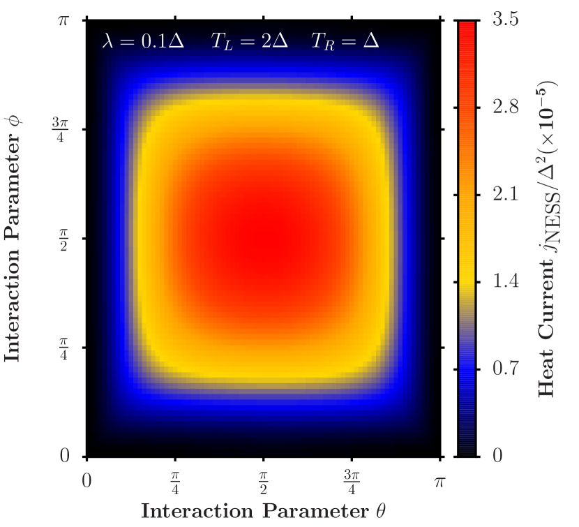
Figure 1: Heat current in the NESS flowing from left ($T_{L}=2\Delta$) towards right bath ($T_{R}=\Delta$) at weak system-bath coupling $\lambda_{L}=\lambda_{R}=\lambda=0.1\Delta$ as a function of the interaction parameters $(\theta,\phi)$. For this calculation we used $\Omega_{L}=\Omega_{R}=\Omega=8\Delta$, $M=6$ and $\gamma_{L}=\gamma_{R}=0.05/\pi$.

II.3 Results

II.3.1 Heat transfer at weak coupling

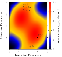
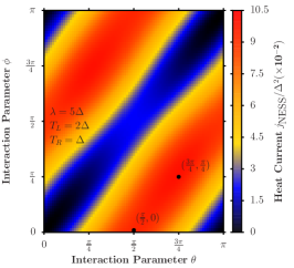
Figure 2: Heat current in the NESS flowing from left ($T_{L}=2\Delta$) towards right bath ($T_{R}=\Delta$) at strong system-bath (from left to right) $\lambda_{L}=\lambda_{R}=\lambda=\Delta,5\Delta,10\Delta$ as a function of the interaction parameters $(\theta,\phi)$. For this calculation we used $\Omega_{L}=\Omega_{R}=\Omega=8\Delta$, $M=6$ and $\gamma_{L}=\gamma_{R}=0.05/\pi$ (note that the values of the current have been rescaled by a different constant value in each panel).

We now turn to investigating the NESS heat currents evaluated from Eq. (II.1) and Eq. (9) in our dual-bath configuration. We are interested in the general case such that $[\hat{S}^{L},\hat{S}^{R}]\neq 0$. Our central system is a single spin degree of freedom

$$\hat{H}_{S}=\Delta\hat{\sigma}^{z},$$ (17)

where $\Delta$ denotes the spin-splitting energy. In order to consider a general set of non-commuting system-bath coupling operators, we define

$$\hat{S}^{L} =\cos(\theta)\hat{\sigma}^{z}+\sin(\theta)\hat{\sigma}^{x},$$

$$\hat{S}^{R} =\cos(\phi)\hat{\sigma}^{z}+\sin(\phi)\hat{\sigma}^{x},$$ (18)

such that we can control non-commutativity between the $\hat{S}_{L,R}$ operators via two angle parameters $(\theta,\phi)$.

At weak coupling, transport takes place through the eigenstates of the system Hamiltonian; which in this case are $\ket{\uparrow}$ and $\ket{\downarrow}$. Effectively, energy transfer is induced by the transitions between the energy levels of the system, and transport is sequential and resonant with the qubit splitting $2\Delta$, see discussion in Appendix C.

In Fig. 1, we present simulations of the heat current in the weak coupling regime, displayed as a function of the interaction angles $(\theta,\phi)$. The current at weak coupling is at its peak whenever $(\theta,\phi)=\left(\frac{\pi}{2},\frac{\pi}{2}\right)$, i.e., when we have $\hat{S}^{L}=\hat{S}^{R}=\hat{\sigma}^{x}$. In this case, the hot bath excites the system, and the qubit medium transfers these excitations to the cold bath. Moving away from the point $(\theta,\phi)=\left(\frac{\pi}{2},\frac{\pi}{2}\right)$ only leads to sub-optimal versions of this process. This is because the contribution to the sequential process weakens and the inclusion of $\hat{\sigma}^{z}$ terms does not contribute to the excitation current that moves through the system.

II.3.2 Heat transfer at strong coupling: the role of the coupling operators

For simplicity, we assume the coupling energy parameter is equal at the two sides, $\lambda=\lambda_{L}=\lambda_{R}$. At weak coupling, we found that the system operator that couples to the baths should be kept close to $\hat{S}^{L}=\hat{S}^{R}=\hat{\sigma}^{x}$ for maximum sequential transport. This, in general, is supported by the fact that heat transfer is mediated by the transitions generated within the system, such that the choice $\hat{S}^{L}=\hat{S}^{R}=\hat{\sigma}^{x}$ is justified.

An interesting behavior is observed as we increase the coupling parameter $\lambda$. In Fig. 2 we show the simulated heat current for the same junction’s parameters as in Fig 1. In this case, however, we increase the coupling energy $\lambda$ to understand strong-coupling behavior. In Fig. 2(left-most panel) we see that increasing the coupling energy for the selected coupling operators in Eq. (II.3.1) means that in order to attain maximum energy transfer one needs to consider different operators other than $\hat{S}^{L}=\hat{S}^{R}=\hat{\sigma}^{x}$. In fact, at stronger values of $\lambda$ as shown in Fig. 2(middle panel) and Fig. 2(right-most panel), the maximum value of the current is continuously attained closer to the points for which the interaction parameters are out of phase by a value of $\pi/2$; that is,

$$\hat{S}^{L} =\cos(\delta)\hat{\sigma}^{z}+\sin(\delta)\hat{\sigma}^{x},$$

$$\hat{S}^{R} =\cos\left(\delta\pm\frac{\pi}{2}\right)\hat{\sigma}^{z}+\sin\left(\delta\pm\frac{\pi}{2}\right)\hat{\sigma}^{x}$$

$$=\mp\sin(\delta)\hat{\sigma}^{z}\pm\cos(\delta)\hat{\sigma}^{x},$$ (19)

where $\delta\in[0,\pi]$ is an arbitrary angle chosen to control the interaction operator.

Although the heat current in Fig. 2 appears to be symmetric under the inversion of the coupling operators $\hat{S}^{L}$ and $\hat{S}^{R}$, a careful comparison shows that this is not the case. Stated differently, we observe a difference in the magnitude of the heat current when the temperatures are exchanged $T_{L}\to T_{R}$ and $T_{R}\to T_{L}$, as long as the coupling operators are different, and even when $\lambda_{L}=\lambda_{R}$. Notably, this difference becomes more pronounced as the temperature bias increases, indicating that the system functions as a heat current rectifier. This observation agrees with the findings reported in Ref. Duan et al. (2020).

These results reveal that non-commuting interaction operators are relevant for maximum heat transfer at strong system-bath coupling energy. At even stronger values of $\lambda$, the heat current resembles the results obtained for $\lambda=10\Delta$ from Fig. 2(right-most panel); with the exception of a narrower maximum along the $(\delta,\delta\pm\frac{\pi}{2})$ points, see Appendix A for further results. We note that in Fig. 2 the absolute values of the energy current are $2-4$ orders of magnitude higher than the weak coupling results in Fig. 1.

II.3.3 Dependence on the coupling energy

We found a stark contrast in the behavior of the overall heat transfer between the weak- and strong-coupling regimes. In the weak-coupling regime, optimal transport requires coupling operators that facilitate transitions between the energy levels of the system. In contrast, in the strong-coupling regime, maximum heat transfer is achieved with coupling operators that do not commute.

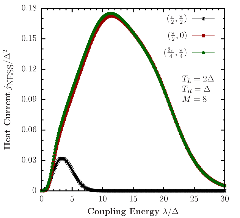
Figure 3: Heat current in the NESS flowing from left ($T_{L}=2\Delta$) towards right bath ($T_{R}=\Delta$) as a function of system-bath coupling $\lambda_{L}=\lambda_{R}=\lambda$. Both interaction angles $(\theta,\phi)=(\frac{\pi}{2},0)$ and $(\theta,\phi)=(\frac{3\pi}{4},\frac{\pi}{2})$, satisfy the condition of Eq. (II.3.2) for which the heat current attains its maximum value at strong system-bath coupling, see Fig. 2. We also present the commuting model with $(\theta,\phi)=(\frac{\pi}{2},\frac{\pi}{2})$, reaching here a lower maximal current at smaller $\lambda$, compared to the other two non-commuting models. For this calculation we used $\Omega_{L}=\Omega_{R}=\Omega=8\Delta$, $M=8$ and $\gamma_{L}=\gamma_{R}=0.05/\pi$.

Following our findings from Sec. II.3.2, we now investigate the behavior of the heat current as a function of the coupling energy parameter $\lambda_{L}=\lambda_{R}=\lambda$. In Fig. 3, we present the heat current as a function of $\lambda$ for three different choices of interaction angles. Let us begin with the non-commuting models, $(\theta,\phi)=(\frac{\pi}{2},0)$ and $(\theta,\phi)=(\frac{3\pi}{4},\frac{\pi}{2})$. In both of these cases, the heat current attains its maximum value (in angle space), see results in Fig. 2(middle panel) and Fig. 2(right-most panel). As a function of $\lambda$, the heat current displays a non-monotonic behavior, initially increasing as $\lambda$ increases, then turning over at sufficiently strong $\lambda$. In Fig. 3, we also display the heat current as a function of $\lambda$ for the commuting operator case $(\theta,\phi)=(\frac{\pi}{2},\frac{\pi}{2})$, for which $\hat{S}^{L}=\hat{S}^{R}=\hat{\sigma}^{x}$. We recall that at weak coupling, these are the coupling operators that lead to optimal heat transfer (see Fig. 1). At intermediate-to-strong coupling, however, we observe that the maximum heat current is an order of magnitude higher if we introduce non-commuting operators on the left and right baths, rather than the more commonly-considered case of $\hat{S}^{L}=\hat{S}^{R}=\hat{\sigma}^{x}$. Furthermore, it is interesting to note that the value of the system-bath coupling $\lambda$ for which the maximum heat current is reached differs (shifts) depending on the system-bath coupling operators chosen, commuting or non-commuting. In the next section, we employ an analytical framework that helps shedding light on this behavior.

In Appendix B, we exemplify convergence trends in reaction coordinate simulations for commuting and non-commuting models with respect to $M$, the number of levels maintained in the reaction coordinate harmonic manifold. Not only are the currents distinct in these cases, but also their numerical convergence is markedly different. This will be rationalized in the next section as well, see Fig. 6.

III Effective Hamiltonian Theory

The transport behavior at weak coupling stands in stark contrast to that observed at strong coupling. In the weak-coupling regime, optimal heat transfer requires system-bath coupling operators that facilitate transitions between the energy levels of a two-level system. This can be achieved with $\hat{S}^{L}=\hat{S}^{R}=\hat{\sigma}^{x}$ for our system Hamiltonian $\hat{H}_{S}=\Delta\hat{\sigma}^{z}$ (see Fig. 1). Interestingly, this is no longer the case whenever the system-baths coupling energy $\lambda$ increases arbitrarily. We find that, instead, one requires operators that do not commute with each other, i.e., $[\hat{S}^{L},\hat{S}^{R}]\neq 0$. Even more interesting is that in our configuration there appears to exist a symmetry, such that if one defines $\hat{S}^{L}$ and $\hat{S}^{R}$ from Eq. (II.3.1), the optimal heat transfer occurs whenever the interaction parameters are out of phase by an angle of $\pi/2$ as in Eq. (II.3.2), see Fig. 2. In what follows, we analyze these findings from the perspective of the Effective Hamiltonian theory.

III.1 Effective system and system-bath operators

The Effective Hamiltonian method, first introduced in Ref. Anto-Sztrikacs et al. (2023a), was developed with the goal of providing analytical insights into strong coupling effects.

It was previously applied to study dynamical, equilibrium and non-equilibrium steady-state problems Anto-Sztrikacs et al. (2023a, b); Brenes et al. (2024); Min et al. (2024); Garwoła and Segal (2024), showing good success in providing qualitative and even quantitative-correct results: For thermal transport problems, the Effective Hamiltonian method was used in Ref. Anto-Sztrikacs et al. (2023a), but only in the case of commuting system-bath operators, where it provided results in excellent agreement with other established numerical simulations Anto-Sztrikacs and Segal (2021). Building on the recent extension of the Effective Hamiltonian method to handle multiple non-commuting operators Garwoła and Segal (2024), we apply it to the current problem in order to provide physical insights.

We introduce the Effective Hamiltonian theory in this section in a brief outline with the most important results. For further details, we refer the reader to Appendix C. For an extensive description and further results, we refer the reader to Refs. Anto-Sztrikacs et al. (2023a, b); Brenes et al. (2024); Min et al. (2024); Garwoła and Segal (2024).

The theory is built on top of the reaction-coordinate mapping, with the Hamiltonian $\hat{H}^{\rm RC}$ from Eq. (II.2). The procedure is to apply the transformation $\hat{H}^{\rm RC-P}=\hat{U}\hat{H}^{\rm RC}\hat{U}^{\dagger}$,

$$\hat{U}=\exp\left[\sum_{\alpha}\frac{\lambda_{\alpha}}{\Omega_{\alpha}}\hat{S}^{\alpha}\left(\hat{a}_{\alpha}^{\dagger}-\hat{a}_{\alpha}\right)\right],$$ (20)

where $\hat{U}$ is known as the polaron transformation. In the present case, there is an important complication whenever the coupling operators $\hat{S}^{\alpha}$ do not commute, which was resolved in Ref. Garwoła and Segal (2024). Following the polaron transformation (20), one considers only the ground-state manifold of the reaction-coordinates in the polaron frame, to obtain an Effective Hamiltonian

$$\hat{H}^{\rm eff}=\hat{Q}_{0}\hat{U}\hat{H}^{\rm RC}\hat{U}^{\dagger}\hat{Q}_{0},$$ (21)

where $\hat{Q}_{0}=\ket{0}\bra{0}$ is the projector operator to the reaction-coordinates’ ground-state manifold. The crucial aspect of this procedure is that it leads to a total system+baths Hamiltonian of the same type as Eq. (II). We obtain Anto-Sztrikacs et al. (2023a); Garwoła and Segal (2024)

$$\hat{H}^{\rm{eff}} =\hat{Q}_{0}\hat{U}\hat{H}_{S}\hat{U}^{\dagger}\hat{Q}_{0}-\sum_{\alpha}\frac{\lambda_{\alpha}^{2}}{\Omega_{\alpha}}\left[\left(\hat{S}^{\alpha}\right)^{2}\right]_{\rm eff}$$

$$+\sum_{\alpha k}\left[\omega_{k,\alpha}\hat{b}_{k,\alpha}^{\dagger}\hat{b}_{k,\alpha}-\frac{2\lambda_{\alpha}f_{k,\alpha}}{\Omega_{\alpha}}\hat{S}^{\alpha}_{\rm eff}(\hat{b}_{k,\alpha}^{\dagger}+\hat{b}_{k,\alpha})\right].$$ (22)

In Eq. (III.1), we recognize the effective system Hamiltonian as

$$\hat{H}^{\rm{eff}}_{S}=\hat{Q}_{0}\hat{U}\hat{H}_{S}\hat{U}^{\dagger}\hat{Q}_{0}-\sum_{\alpha}\frac{\lambda_{\alpha}^{2}}{\Omega_{\alpha}}\left[\left(\hat{S}^{\alpha}\right)^{2}\right]_{\rm eff}.$$ (23)

The endeavor then becomes to evaluate both $\hat{H}^{\rm eff}_{S}$ and $\hat{S}^{\alpha}_{\rm eff}$ explicitly, so one may employ these results to understand the underlying strong-coupling effects from the perspective of a weak-coupling theory. Note that the second term in the above equation contributes a constant in the present study.

In general, the Effective Hamiltonian theory embeds the effects of strong coupling onto both system and system-bath coupling operators.

Figure 4: Dressing functions with respect to the coupling energy $\lambda/\Omega$.

We are interested in two cases: the commuting case in which $(\theta,\phi)=(\frac{\pi}{2},\frac{\pi}{2})$ and the non-commuting case for which we observe the optimal heat transfer at strong coupling $(\theta,\phi)=(\delta,\delta\pm\frac{\pi}{2})$.

The former has been investigated in previous works Anto-Sztrikacs et al. (2023a, b); Brenes et al. (2024); Min et al. (2024) and leads to the expressions (with $\lambda=\lambda_{\alpha}$ and $\Omega=\Omega_{\alpha}$)

$$\hat{H}_{S}^{\rm eff} =e^{-\frac{4\lambda^{2}}{\Omega^{2}}}\Delta\hat{\sigma}^{z},$$

$$\hat{S}^{\alpha}_{\rm eff} =\hat{S}^{\alpha}=\hat{\sigma}^{x};\quad(\theta,\phi)=(\pi/2,\pi/2).$$ (24)

From the Effective Hamiltonian theory we observe that the effect of strong coupling is to suppress the spin-splitting energy of the system Hamiltonian, while the system-bath coupling operator remains as in the weakly-coupled case Anto-Sztrikacs and Segal (2021). This approach is very powerful in explaining the heat current behavior in Fig. 3: At vanishing $\lambda$, the current tends to zero as it is this coupling energy that mediates energetic transitions. At large $\lambda$, the spin-splitting energy vanishes, therefore inhibiting transitions from happening, which results in no heat current flowing through the system. There exists a maximum at a finite coupling $\lambda$ whenever the coupling is optimal with respect to the transitions that can be mediated by the system.

We next focus on the case where $\hat{S}^{L}$ and $\hat{S}^{R}$ do not commute. The calculation involved is more complicated in this case. We show in Appendix C that (with $\lambda=\lambda_{\alpha}$ and $\Omega=\Omega_{\alpha}$)

$$\hat{H}_{S}^{\rm eff} =f\left(\frac{\lambda}{\Omega}\right)\Delta\hat{\sigma}^{z},$$

$$\hat{S}^{\alpha}_{\rm eff} =f\left(\frac{\lambda}{\Omega}\right)\hat{S}^{\alpha},\quad\forall(\theta,\phi)=\left(\delta,\delta\pm\frac{\pi}{2}\right),$$ (25)

where $f(x)=1-x\sqrt{2}F(x\sqrt{2})$ and $F(y)=e^{-y^{2}}\int_{0}^{y}{\rm d}te^{t^{2}}$ is the Dawson integral.

In Fig. 4 we display both dressing functions, i.e., the pre-factors in front of the system Hamiltonian that embed the effects of strong coupling onto the system for different choices of coupling operators. Whenever the coupling operators $\hat{S}_{L}=\hat{S}_{R}$, we obtain an exponential decay that explains the maximum and the turnover observed in the heat current (Fig. 3, black curve). As mentioned earlier, it is related to the vanishing spin-splitting at large $\lambda$. For the non-commuting case, for which we have chosen the points at which the heat current attains its maximum values $(\theta,\phi)=(\delta,\delta\pm\frac{\pi}{2})$, the dressing function illustrates that neither the spin-splitting energy nor the coupling operators themselves vanish in the limit of large $\lambda$. This would suggest that the heat current remains finite in the limit $\lambda\to\infty$, in apparent contradiction to our findings in Fig. 3 (green and red curves). We investigate this further in the next section.

Irrespective of this, the Effective Hamiltonian theory for non-commuting operators reveals an underlying symmetry that occurs whenever $(\theta,\phi)=(\delta,\delta\pm\frac{\pi}{2})$, such that both system Hamiltonian and system-baths coupling operators get dressed with the same dressing function.

III.2 Currents from the Effective Hamiltonian theory

Armed with the Effective Hamiltonian formalism, we attempt to understand strong-coupling thermodynamics from the perspective of a weak-coupling theory.

Figure 5: Heat current in the NESS flowing from left ($T_{L}=\Delta$) towards right bath ($T_{R}=\Delta/2$) as a function of system-bath coupling $\lambda_{L}=\lambda_{R}=\lambda$ for three different interaction parameters $(\theta,\phi)=(\frac{\pi}{2},\frac{\pi}{2})$, $(\theta,\phi)=(\frac{\pi}{2},0)$ and $(\theta,\phi)=(\frac{3\pi}{4},\frac{\pi}{4})$. In each case we display the reaction-coordinate calculations as in Fig. 3 and those predicted by our Effective Hamiltonian model. For this calculation we used $\Omega_{L}=\Omega_{R}=\Omega=8\Delta$, $M=8$ and $\gamma_{L}=\gamma_{R}=0.05/\pi$.

For the heat current, the procedure is the same as highlighted in Sec. II.1 and Sec. II.2, with the exception that now we use the Effective Hamiltonian, Eq. (III.1), which involves both an effective system Hamiltonian and effective system-bath coupling operators. We remark that this is done in such a way that the Effective Hamiltonian introduces the effects of strong coupling while the entire system+baths configuration remains at weak coupling via our Markovian embedding.

Fig. 5 displays the heat current as a function of the system-bath coupling energy $\lambda=\lambda_{L}=\lambda_{R}$ for three different interaction operators with angles $(\theta,\phi)=(\frac{\pi}{2},\frac{\pi}{2})$, $(\theta,\phi)=(\frac{\pi}{2},0)$ and $(\theta,\phi)=(\frac{3\pi}{4},\frac{\pi}{4})$. For this calculation, we chose $T_{L}=\Delta$ and $T_{R}=\Delta/2$. In Fig. 5 we display the reaction-coordinate results and their corresponding Effective Hamiltonian counterparts. We start by remarking that as the mean temperature and the temperature gradient change, the interaction parameters $(\theta,\phi)$ now introduce another layer of parameters that need to be optimized to achieve the optimal heat current. From Fig. 5 we observe that $(\theta,\phi)=(\frac{3\pi}{4},\frac{\pi}{4})$ produces a higher value of the maximum current than the model $(\theta,\phi)=(\frac{\pi}{2},0)$, although in both cases the condition $(\theta,\phi)=(\delta,\delta\pm\frac{\pi}{2})$ is satisfied. Irrespective of this, in both cases we observe similar trends for the heat current as a function of $\lambda$, as in Fig. 2 and Fig. 3.

With respect to the heat current predictions of the effective model, we see a stark contrast depending on the chosen system-bath operators $\hat{S}^{\alpha}$. For the case $(\theta,\phi)=(\frac{\pi}{2},\frac{\pi}{2})$, the effective model correctly reproduces the heat current of the full reaction-coordinate model and therefore provides an intuitive analytical understanding of the relevant strong-coupling thermodynamics. The approximation remains valid as long as the condition $\Omega\gtrsim\lambda,T$ is satisfied Anto-Sztrikacs et al. (2023a). The intuition behind this is that when $\Omega\lesssim\lambda,T$, additional important transport channels contribute, which are not accounted for with the effective model. This limitation arises because the model relies on a ground-state manifold truncation of the reaction coordinate in the polaron frame. However, when $[\hat{S}^{L},\hat{S}^{R}]\neq 0$, we observe in Fig. 5 that our effective treatment does not adequately replicate the behavior of the heat current. This is an indication that the transport channels are starkly different depending on the chosen system-bath coupling operators and their commutativity. In the dissipative-decoherence model $(\theta,\phi)=(\frac{\pi}{2},0)$, the Effective Hamiltonian predicts no current flowing through the system, which we derive in Appendix C. This stands in complete contrast to reaction coordinate simulations. Second, for the model $(\theta,\phi)=(\frac{3\pi}{4},\frac{\pi}{4})$, the Effective Hamiltonian method provides two peaks, albeit the second one missing the height and position of reaction-coordinate simulations.

Figure 6: First 10 eigenvalues of the system reaction-coordinate Hamiltonian $\hat{H}^{\rm{RC}}_{S}$ [Eq. (14)] transformed by the unitary operator $\hat{U}$ [Eq. (20)] as a function of the system-baths coupling energy $\lambda$. Two cases are displayed. The top panel shows the eigenvalues for commuting system-baths operators with interaction parameters $(\theta,\phi)=(\frac{\pi}{2},\frac{\pi}{2})$, while the bottom panel shows the non-commuting case $(\theta,\phi)=(\frac{\pi}{2},0)$.

To understand the failure of the Effective Hamiltonian theory for studying heat currents under non-commuting operators, in Fig. 6 we display the first few eigenvalues of the polaron-transformed reaction coordinate Hamiltonian, $\hat{H}^{\rm{RC-P}}_{S}=\hat{U}\hat{H}^{\rm{RC}}_{S}\hat{U}^{\dagger}$ defined from Eq. (14) and Eq. (20). For this calculation, we approximate the polaron transformation by truncating the reaction coordinate modes to $M=40$, then looking at the first few eigenvalues as shown in Fig. 6. We have confirmed that the eigenvalues have converged with this value of $M$. Fig. 6 reveals an important aspect when considering the case $(\theta,\phi)=(\frac{\pi}{2},\frac{\pi}{2})$. In this model, the first two levels do not cross excited states and their gap to higher levels remains fixed as $\lambda$ increases. This justifies the truncation made in the Effective Hamiltonian treatment, as long as $\Omega\gtrsim\lambda,T$. As a result, we obtain a good approximation for the heat current as observed in Fig. 5. On the other hand, we observe that when $[\hat{S}^{L},\hat{S}^{R}]\neq 0$, multiple excited states become relevant once $\lambda$ increases, given that the gap between levels is reduced, even leading to level crossing. These results are an indication that an Effective Hamiltonian model, which considers only the ground-state manifold of the polaron-transformed reaction-coordinate Hamiltonian, does not provide a full picture of the transport properties for $\lambda/\Delta\gtrsim 4$.

In terms of transport mechanisms, for the family of models with ($\theta$,$\phi$) = ($\delta$,$\delta\pm\pi/2$), the current from the reaction coordinate simulations attains its maximum for $\lambda\approx 2\Omega$. We recall that $\Omega$ corresponds to the characteristic frequency of the bath, translating to the frequency of the reaction coordinate. The heat current peaks at a coupling energy value of approximately that frequency, suggesting that heat exchange is dominated by processes that exchange this amount of energy. In some cases, one can also discern a small “hump” at $\lambda\approx 2\Delta$ (see Fig. 5), in addition to the strong peak at $\lambda\approx 2\Omega$. Our interpretation is that there are two transport channels at play, a transport channel utilizing the spin gap, and a higher-order transport channel with a direct energy transfer between the baths, mediated by the spin system, but without a physical population transfer to it. Importantly (see Appendix C), the Effective Hamiltonian framework is only capable in capturing transport through the central spin, and it cannot capture processes at higher frequencies, which take advantage of the reaction coordinate modes. The two-peak structure that the Effective Hamiltonian generates in Fig. 5 emerges due to the non-monotonicity of the dressing functions of the spin splitting and coupling operators, rather than the competition of two transport channels (see Fig. 4).

With respect to quantum heat transfer in spin-boson models, we conclude that the Effective Hamiltonian method captures well the commuting case investigated here, even at strong coupling. For non-commuting operators, the dressing functions in the Effective Hamiltonian reflects the symmetry of transport with respect to $\pi/2$ shift in the angles of the coupling operators, Eq. (III.1). However, due to the truncation to the ground state manifold of the reaction coordinates, the Effective Hamiltonian technique does not capture thermal transport through higher transitions than the central spin’s gap. These processes dominate transport in non-commuting models at strong coupling. The method thus provides quantitative correct predictions only up to $\lambda\approx\Delta$, but is expected to perform better at low temperatures when transport is controlled by low-energy processes.

It is interesting to note that the Effective Hamiltonian approach showed success in capturing the equilibrium state of a spin system coupled to non-commuting baths Garwoła and Segal (2024). It is clear that the NESS poses a new challenge to the Effective Hamiltonian method when non-commuting operators are at play, calling for future developments.

IV Conclusions

We conducted a numerical investigation of quantum heat transfer between two bosonic reservoirs mediated by a central spin degree of freedom. Our focus was on optimizing the heat current by manipulating the system-bath coupling operators. The study explored a broad range of coupling regimes, spanning from weak to ultrastrong interactions, while allowing the coupling operators to the two reservoirs to be non-commuting. Jointly, these features introduce significant technical challenges that are difficult to address using standard perturbative or non-perturbative methods.

To analyze this setup, we employed the reaction coordinate Markovian embedding method. The key finding of our study is that the optimal coupling operators for maximizing the heat current vary across different interaction regimes. In the weak coupling regime, the heat current is maximized when the central spin couples to the baths through identical operators that facilitate sequential-resonant transport, specifically $\hat{\sigma}^{x}$. In contrast, in the strong coupling regime, the heat current is optimized using a specific arrangement of non-commuting coupling operators. Specifically, in this regime, the system should couple to the two baths with a combination of spin components, $\hat{\sigma}^{x}$ and $\hat{\sigma}^{z}$, with their relative weight dictated by angle measures $\delta$ for one contact and $\delta\pm\pi/2$ for the other.

The Effective Hamiltonian framework was successfully used in several previous studies to capture non-perturbative system-bath coupling phenomena, and even in the ultrastrong coupling limit. Here, we learned that one should be cautious with the Effective Hamiltonian treatment, as there are models where it critically fails to capture the relevant NESS behavior. Future work will be devoted to extending this treatment to allow its application on a broader range of models.

Our optimization of the heat current was carried out under the assumption of a relatively small temperature bias across the junction. It is important to emphasize the richness of the transport model: evaluating the heat current under a high bias may yield a different set of coupling operators optimized for maximizing the current in that regime. Furthermore, we limited ourselves to the case of identical contacts by using the same spectral functions $J(\omega)$ and coupling energies $\lambda$. Introducing asymmetry at the contacts could provide additional control over both the magnitude and behavior of the quantum heat current in nanoscale junctions. Finally, it would be interesting to further examine the current noise in these non-equilibrium devices and identify setups of high current with low noise levels.

Appendix A Heat transfer at stronger values of system-baths coupling energy

Figure 7: Heat current in the NESS flowing from left ($T_{L}=2\Delta$) towards right bath ($T_{R}=\Delta$) at strong system-bath coupling $\lambda_{L}=\lambda_{R}=\lambda=20\Delta$ as a function of the interaction parameters $(\theta,\phi)$. For this calculation we used $\Omega_{L}=\Omega_{R}=\Omega=8\Delta$, $M=6$ and $\gamma_{L}=\gamma_{R}=0.05/\pi$.

We present here an additional example of the dependence of the heat current on the two angle parameters $\theta$ and $\phi$, which control the coupling operators of the system to the baths. Extending Fig. 1 and Fig. 2, Fig. 8 examines the case where the coupling energy is as large as $\lambda=20\Delta$. The results reveal that the heat current is maximized when $(\theta,\phi)=(\delta,\delta\pm\pi/2)$, but it rapidly decreases as the parameters deviate from this configuration. This behavior indicates that in the ultrastrong coupling limit, the system becomes insulating outside this symmetry.

Appendix B Convergence of the reaction-coordinate calculations with respect to level truncation

Figure 8: Comparison of the NESS heat currents with respect to reaction-coordinate level truncation $M$. The heat current is flowing from the left ($T_{L}=1.5\Delta$) towards the right bath ($T_{R}=0.5\Delta$), and it is presented here as a function of the coupling energy $\lambda=\lambda_{L}=\lambda_{R}$ for two different interaction parameters $(\theta,\phi)=\left(\frac{\pi}{2},\frac{\pi}{2}\right)$ (top) and $(\theta,\phi)=\left(\frac{\pi}{4},-\frac{\pi}{4}\right)$ (bottom). For this calculation we used $\Omega_{L}=\Omega_{R}=\Omega=8\Delta$ and $\gamma_{L}=\gamma_{R}=0.05/\pi$.

In this Appendix, we discuss the convergence of reaction-coordinate simulations with respect to the truncation of the RC manifold. In our model we extract two RCs, one from each bath, where for simplicity we assume that the baths are characterized by identical spectral functions with the same parameters: $\Omega$, $\gamma$ and $\lambda$; as the characteristic frequency of the baths, width of the spectral function and coupling energy to the system, respectively. Given that extracted RCs are identical, we assume that similar truncations should be done on both baths, i.e., we maintain $M$ levels for each RC.

In Fig. 8, we present simulation results. In the top panel, both baths are coupled to the system through the $\hat{\sigma}^{x}$ operator. In this model, which was previously examined in Ref. Anto-Sztrikacs and Segal (2021) using the reaction coordinate method, convergence with respect to $M$ is easily achieved, with some small deviations showing up as one increases $\lambda$ to $\lambda/\Delta\geq 6$. However, in that regime, the current is strongly suppressed, and thus these deviations have a small impact on the current. The exceptional success and convergence of RC simulations can be rationalized by the analysis of level spacings, which, as illustrated in Fig. 6(top), shows the robustness of the energy spectrum even at strong coupling Anto-Sztrikacs and Segal (2021).

Moving on to the bottom panel of Fig. 8, here we analyze the case with non-commuting system operators coupled to the two baths, with an angle difference of $\pi/2$. Focusing on convergence trends with respect to $M$, it is clear that: (i) At weak to intermediate coupling, up to $\lambda/\Delta\approx 5$, we reach excellent convergence with $M=4$ capturing results. (ii) Close to the maximum, at $\lambda/\Delta\approx 10$, we note that the current is monotonically converging as we increase $M$. (iii) In the ultrastrong coupling regime, $\lambda/\Delta>20$, while all curves show similar trends (suppression of the heat current with increasing coupling energy), it is necessary to maintain more levels in each RC to converge.

The challenge in achieving convergence under general coupling operators can once again be understood by examining the eigenenergies of the RC Hamiltonian. As shown in Fig. 6(bottom), increasing $\lambda$ causes energy levels to approach and cross each other. This behavior requires the inclusion of a large number of RC levels to accurately cover the relevant energetic window, which is determined by the ratio $\Omega/\Delta$ and $\Omega/T_{L,R}$.

Appendix C Details on the Effective Hamiltonian theory

In this Appendix, we present derivations of the effective system operators in different cases and derive analytical formulas for the heat current for the effective models discussed in the main text. While the method failed to reproduce the strong coupling trends of heat currents for general non-commuting operators, we detail it here for several reasons. First, it provides qualitative (and even quantitative) correct results beyond the strict weak coupling limit, see Fig. 5. This is because the method correctly captures transport behavior thorough the central spin—though it is missing additional transport pathways. Second, the analytical expressions of the Effective Hamiltonian method provide us with a good understanding of the physics controlling transport at low frequencies. Third, the effective method is expected to become more accurate at low temperatures, when transport through high energy levels is suppressed.

The Effective Hamiltonian theory in the case of non-commuting system operators was developed in details in Ref. Garwoła and Segal (2024). We present here the technical steps relevant for our model.

We need to evaluate the following two integrals over momentum. Each integral is two dimensional, as it covers momentum related to each reaction coordinate,

$$(\hat{\sigma}^{z})^{\text{eff}} =\int\hat{U}_{P}(\tilde{\bm{p}})\hat{\sigma}^{z}\hat{U}_{P}^{\dagger}(\tilde{\bm{p}})\prod_{\alpha=L,R}\frac{e^{-\tilde{p}_{\alpha}^{2}}d\tilde{p}_{\alpha}}{\sqrt{\pi}},$$ (26)

$$(\hat{\sigma}^{x})^{\text{eff}} =\int\hat{U}_{P}(\tilde{\bm{p}})\hat{\sigma}^{x}\hat{U}_{P}^{\dagger}(\tilde{\bm{p}})\prod_{\alpha=L,R}\frac{e^{-\tilde{p}_{\alpha}^{2}}d\tilde{p}_{\alpha}}{\sqrt{\pi}}.$$

For coupling operators defined by the following two angle parameters, $\hat{S}^{L}=\cos(\theta)\hat{\sigma}^{z}+\sin(\theta)\hat{\sigma}^{x}$ and $\hat{S}^{R}=\cos(\phi)\hat{\sigma}^{z}+\sin(\phi)\hat{\sigma}^{x}$, the unitary polaron transformation is given by

$$\hat{U}_{P}(\bm{\tilde{p}}) =\exp\left(-i\sqrt{2}\frac{\lambda}{\Omega}\sum_{\alpha}\tilde{p}_{\alpha}\hat{S}^{\alpha}\right)$$ (27)

$$=\hat{\sigma}^{0}\cosh\left(\sqrt{2}\frac{\lambda}{\Omega}\sqrt{-2\tilde{p}_{L}\tilde{p}_{R}\cos(\theta-\phi)-\tilde{p}_{L}^{2}-\tilde{p}_{R}^{2}}\right)$$

$$-\hat{\sigma}^{x}\frac{i\left(\sin(\theta)\tilde{p}_{L}+\tilde{p}_{R}\sin(\phi)\right)\sinh\left(\sqrt{2}\frac{\lambda}{\Omega}\sqrt{-2\tilde{p}_{L}\tilde{p}_{R}\cos(\theta-\phi)-\tilde{p}_{L}^{2}-\tilde{p}_{R}^{2}}\right)}{\sqrt{-2\tilde{p}_{L}\tilde{p}_{R}\cos(\theta-\phi)-\tilde{p}_{L}^{2}-\tilde{p}_{R}^{2}}}$$

$$-\hat{\sigma}^{z}\frac{i\left(\cos(\theta)\tilde{p}_{L}+\tilde{p}_{R}\cos(\phi)\right)\sinh\left(\sqrt{2}\frac{\lambda}{\Omega}\sqrt{-2\tilde{p}_{L}\tilde{p}_{R}\cos(\theta-\phi)-\tilde{p}_{L}^{2}-\tilde{p}_{R}^{2}}\right)}{\sqrt{-2\tilde{p}_{L}\tilde{p}_{R}\cos(\theta-\phi)-\tilde{p}_{L}^{2}-\tilde{p}_{R}^{2}}}.$$

This expression was derived using $\lambda=\lambda_{L,R}$ and $\Omega=\Omega_{L,R}$.

C.1 Dressing of operators in the Effective Hamiltonian framework for $(\theta,\phi)=(\delta,\delta\pm\frac{\pi}{2})$

We now focus on the special case of $(\theta,\phi)=(\delta,\delta\pm\frac{\pi}{2})$. In this case, the polaron operator simplifies to

$$\hat{U}_{P}(\bm{\tilde{p}}) =\hat{\sigma}^{0}\cos\left(\sqrt{2}\frac{\lambda}{\Omega}\sqrt{\tilde{p}_{L}^{2}+\tilde{p}_{R}^{2}}\right)$$ (28)

$$-\hat{\sigma}^{x}\frac{i\sin\left(\sqrt{2}\frac{\lambda}{\Omega}\sqrt{\tilde{p}_{L}^{2}+\tilde{p}_{R}^{2}}\right)\left(\sin(\delta)\tilde{p}_{L}\pm\cos(\delta)\tilde{p}_{R}\right)}{\sqrt{\tilde{p}_{L}^{2}+\tilde{p}_{R}^{2}}}$$

$$-\hat{\sigma}^{z}\frac{i\sin\left(\sqrt{2}\frac{\lambda}{\Omega}\sqrt{\tilde{p}_{L}^{2}+\tilde{p}_{R}^{2}}\right)\left(\cos(\delta)\tilde{p}_{L}\mp\sin(\delta)\tilde{p}_{R}\right)}{\sqrt{\tilde{p}_{L}^{2}+\tilde{p}_{R}^{2}}}.$$

We simplify the integrals in Eq. (26) by using the substitution $\tilde{p}_{L}=r\cos(\alpha)$, $\tilde{p}_{R}=r\sin(\alpha)$. We arrive at

$$(\hat{\sigma}^{z})^{\text{eff}} =\int_{0}^{\infty}re^{-r^{2}}dr\int_{0}^{2\pi}\frac{d\alpha}{\pi}{\Big{\{}}\hat{\sigma}^{z}\Big{[}\cos^{2}(\sqrt{2}\frac{\lambda}{\Omega}r)+\cos\left(2(\alpha\pm\delta)\right)\sin^{2}(\sqrt{2}\frac{\lambda}{\Omega}r)\Big{]}$$ (29)

$$+\hat{\sigma}^{x}\Big{[}\pm\sin\left(2(\alpha\pm\delta)\right)\sin^{2}\left(\sqrt{2}\frac{\lambda}{\Omega}r\right)\Big{]}$$

$$+\hat{\sigma}^{y}\Big{[}\mp 2\sin(\alpha\pm\delta)\sin\left(\sqrt{2}\frac{\lambda}{\Omega}r\right)\Big{]}{\Big{\}}},$$

$$(\hat{\sigma}^{x})^{\text{eff}} =\int_{0}^{\infty}re^{-r^{2}}dr\int_{0}^{2\pi}\frac{d\alpha}{\pi}{\Big{\{}}\hat{\sigma}^{z}\left[\pm\sin\left(2(\alpha\pm\delta)\right)\sin^{2}\left(\sqrt{2}\frac{\lambda}{\Omega}r\right)\right]$$

$$+\hat{\sigma}^{x}\left[\cos^{2}\left(\sqrt{2}\frac{\lambda}{\Omega}r\right)-\cos\left(2(\alpha\pm\delta)\right)\sin^{2}(\sqrt{2}\frac{\lambda}{\Omega}r)\right]$$

$$+\hat{\sigma}^{y}\left[\cos(\alpha\pm\delta)\sin\left(2\sqrt{2}\frac{\lambda}{\Omega}r\right)\right]{\Big{\}}}.$$

Integration over the angle $\alpha$ greatly simplifies the above expressions, reaching

$$(\hat{\sigma}^{z})^{\text{eff}} =\hat{\sigma}^{z}\int_{0}^{\infty}2e^{-r^{2}}r\cos^{2}\left(\sqrt{2}\lambda r\right)dr,\,\,\,\,\,\,\,\,\,(\hat{\sigma}^{x})^{\text{eff}} =\hat{\sigma}^{x}\int_{0}^{\infty}2e^{-r^{2}}r\cos^{2}\left(\sqrt{2}\lambda r\right)dr.$$ (30)

We can express the above integrals as Dawson functions, as presented in the main text, below Eq. (III.1).

These dressing of operators impact the Hamiltonian in two substantial ways. First, the dressing of $\hat{\sigma}^{z}$ translates to dressing of the spin energy splitting $\Delta$, as demonstrated in Eq. (III.1) and in Fig. 4. The dressing is non-monotonic, but generally, its impact is to reduce $\Delta$ to ultimately $\Delta/2$ at the ultrastrong coupling limit. The second impact of the dressing is to modify the system-bath coupling energies. These modification is symmetric-identical when the spectral functions are assumed the same, see Eq. (III.1). Both these aspects should impact the heat current, as we show in the next subsection. Particularly, a suppression of the splitting should reduce the sequential heat current with each transition carrying less energy.

C.2 Heat current in the effective Hamiltonian framework

We proceed to find the analytical expressions for the steady state heat current using the Redfield equation (II.1). Once we find the steady state population from the Redfield equation, we compute the heat current, flowing between the system and the left bath,

$$j_{\text{NESS}}=-2\tilde{\Delta}\Big{(}k_{L}^{\downarrow}\rho_{22}^{\text{SS}}-k_{L}^{\uparrow}\rho_{11}^{\text{SS}}\Big{)}.$$ (31)

According to our sign convention, the heat current is positive when flowing into the system. Here, $\tilde{\Delta}$ is the suppressed system energy splitting, $k_{L}^{\downarrow}$ and $k_{L}^{\uparrow}$ are the rates of transition from the excited to the ground state of the system and vice versa. These rate stand as a general notation.

Below, we derive the explicit expressions for these rates for each model in the language of the Redfield tensor.

It is sufficient to find the heat current between the system and the left bath, since in the NESS it is equal to minus the heat current between the system and the right bath. We focus here on deriving analytical expressions for the heat current for models examined in Section III.

C.2.1 The commuting model, $(\phi,\theta)=(\frac{\pi}{2},\frac{\pi}{2})$

We focus on the case $(\theta,\phi)=(\frac{\pi}{2},\frac{\pi}{2})$. The Redfield equations for the diagonal elements of the reduced density matrix are given by

$$\frac{d}{dt}\rho_{11}(t) =-\sum_{\alpha=L,R}\Big{(}[R_{12,21}^{\alpha,\text{eff}}(\omega_{12})+R_{12,21}^{\alpha,*,\text{eff}}(\omega_{12})]\rho_{11}(t)-\big{[}R_{21,12}^{\alpha,\text{eff}}(\omega_{21})+R_{21,12}^{\alpha,*,\text{eff}}(\omega_{21})\big{]}\rho_{22}(t)\Big{)}$$ (32)

$$= -2\sum_{\alpha=L,R}\text{Re}\Big{(}[R_{12,21}^{\alpha,\text{eff}}(\omega_{12})+R_{21,12}^{\alpha,\text{eff}}(\omega_{21})]\rho_{11}(t)-R_{21,12}^{\alpha,\text{eff}}(\omega_{21})\Big{)},$$

and

$$\frac{d}{dt}\rho_{22}(t) =-\sum_{\alpha=L,R}\Big{(}[R_{21,12}^{\alpha,\text{eff}}(\omega_{21})+R_{21,12}^{\alpha,*,\text{eff}}(\omega_{21})]\rho_{22}(t)-\big{[}R_{12,21}^{\alpha,\text{eff}}(\omega_{12})+R_{12,21}^{\alpha,*,\text{eff}}(\omega_{12})\big{]}\rho_{11}(t)\Big{)}$$ (33)

$$=-2\sum_{\alpha=L,R}\text{Re}\Big{(}[R_{21,12}^{\alpha,\text{eff}}(\omega_{21})+R_{12,21}^{\alpha,\text{eff}}(\omega_{12})]\rho_{22}(t)-R_{12,21}^{\alpha,\text{eff}}(\omega_{12})\Big{)}.$$

We readily find the steady state diagonal elements of the reduced density matrix,

$$\rho_{11}^{SS} =\frac{\sum_{\alpha=L,R}\text{Re}\Big{(}R_{21,12}^{\alpha,\text{eff}}(\omega_{21})\Big{)}}{\sum_{\alpha=L,R}\text{Re}\Big{(}[R_{12,21}^{\alpha,\text{eff}}(\omega_{12})+R_{21,12}^{\alpha,\text{eff}}(\omega_{21})]\Big{)}},$$ (34)

and

$$\rho_{22}^{SS} =\frac{\sum_{\alpha=L,R}\text{Re}\Big{(}R_{12,21}^{\alpha,\text{eff}}(\omega_{12})\Big{)}}{\sum_{\alpha=L,R}\text{Re}\Big{(}[R_{21,12}^{\alpha,\text{eff}}(\omega_{21})+R_{12,21}^{\alpha,\text{eff}}(\omega_{12})]\Big{)}}.$$ (35)

The steady state heat current is equal to

$$j_{\text{NESS}} =-4\tilde{\Delta}\text{Re}\Big{(}R_{12,21}^{L,\text{eff}}(\omega_{21})\rho_{22}^{\text{SS}}-R_{21,12}^{L,\text{eff}}(\omega_{12})\rho_{11}^{\text{SS}}\Big{)}.$$ (36)

We assume that $\lambda_{L}=\lambda_{R}=\lambda$. In the present model, the dressing leads to $\tilde{\Delta}=\Delta\exp(-4\frac{\lambda^{2}}{\Omega^{2}})$. Furthermore, the elements in the dissipator are, for both $\alpha=L,R$,

$$R_{12,21}^{\alpha,\text{eff}}(\omega_{12}) =R_{21,12}^{\alpha,\text{eff}}(\omega_{12}),$$ (37)

$${\rm Re}\left(R_{12,21}^{\alpha,\text{eff}}(\omega_{12})\right)=\Gamma_{\text{eff}}^{\alpha}(\omega_{12})=\pi J_{\text{eff}}^{\alpha}(2\tilde{\Delta})n^{\alpha}(2\tilde{\Delta}),$$

$$R_{12,21}^{\alpha,\text{eff}}(\omega_{21}) =R_{21,12}^{\alpha,\text{eff}}(\omega_{21}),$$

$${\rm Re}\left(R_{12,21}^{\alpha,\text{eff}}(\omega_{21})\right)=\Gamma_{\text{eff}}^{\alpha}(\omega_{21})=\pi J_{\text{eff}}^{\alpha}(2\tilde{\Delta})\big{(}n^{\alpha}(2\tilde{\Delta})+1\big{)},$$

where we define

$$J_{\text{eff}}^{\alpha}(\omega)=\frac{4\lambda^{2}}{\Omega^{2}}J_{\text{RC}}^{\alpha}(\omega).$$ (38)

Altogether, plugging the steady state populations and the rate constants in Eq. (36), we obtain the heat current

$$j_{\text{NESS}} =-4\pi\tilde{\Delta}\left[\frac{J_{\text{eff}}^{L}(2\tilde{\Delta})\big{(}n^{L}(2\tilde{\Delta})+1\big{)}\sum_{\alpha=L,R}J_{\text{eff}}^{\alpha}(2\tilde{\Delta})n^{\alpha}(2\tilde{\Delta})-J_{\text{eff}}^{L}(2\tilde{\Delta})n^{L}(2\tilde{\Delta})\sum_{\alpha=L,R}J_{\text{eff}}^{\alpha}(2\tilde{\Delta})\big{(}n^{\alpha}(2\tilde{\Delta})+1\big{)}}{\sum_{\alpha=L,R}J_{\text{eff}}^{\alpha}(2\tilde{\Delta})\big{(}2n^{\alpha}(2\tilde{\Delta})+1\big{)}}\right]$$ (39)

$$=-4\pi\tilde{\Delta}\left[\frac{J_{\text{eff}}^{L}(2\tilde{\Delta})J_{\text{eff}}^{R}(2\tilde{\Delta})\Big{(}n^{R}(2\tilde{\Delta})\big{(}n^{L}(2\tilde{\Delta})+1\big{)}-n^{L}(2\tilde{\Delta})\big{(}n^{R}(2\tilde{\Delta})+1\big{)}\Big{)}}{\sum_{\alpha=L,R}J_{\text{eff}}^{\alpha}(2\tilde{\Delta})\big{(}2n^{\alpha}(2\tilde{\Delta})+1\big{)}}\right]$$

$$=\frac{4\pi\tilde{\Delta}J_{\text{eff}}^{L}(2\tilde{\Delta})J_{\text{eff}}^{R}(2\tilde{\Delta})\left[n^{L}(2\tilde{\Delta})-n^{R}(2\tilde{\Delta})\right]}{\sum_{\alpha=L,R}J_{\text{eff}}^{\alpha}(2\tilde{\Delta})\big{[}2n^{\alpha}(2\tilde{\Delta})+1\big{]}}.$$

This result was originally derived in Ref. Segal and Nitzan (2005); Segal (2006) at weak coupling, and later presented for the effective framework in Ref. Anto-Sztrikacs and Segal (2021).

C.2.2 The dissipative-decoherence model, $(\theta,\phi)=(\frac{\pi}{2},0)$

In the case where $(\theta,\phi)=(\frac{\pi}{2},0)$, the non-zero elements of the Redfield tensor are different for the left and right baths. The equations of motion for the populations are

$$\frac{d}{dt}\rho_{11}(t) =-2\text{Re}\Big{(}R_{12,21}^{L,\text{eff}}(\omega_{12})\rho_{11}(t)-R_{21,12}^{L,\text{eff}}(\omega_{21})\rho_{22}(t)\Big{)}$$ (40)

$$\;-2\text{Re}\Big{(}R_{11,11}^{R,\text{eff}}(\omega_{11})\rho_{11}(t)-R_{11,11}^{R,\text{eff}}(\omega_{11})\rho_{11}(t)\Big{)}$$

$$=-2\text{Re}\Big{(}[R_{12,21}^{L,\text{eff}}(\omega_{12})+R_{21,12}^{L,\text{eff}}(\omega_{21})]\rho_{11}(t)-R_{21,12}^{L,\text{eff}}(\omega_{21})\Big{)},$$

and

$$\frac{d}{dt}\rho_{22}(t) =-2\text{Re}\Big{(}R_{21,12}^{L,\text{eff}}(\omega_{21})\rho_{22}(t)-R_{12,21}^{L,\text{eff}}(\omega_{12})\rho_{11}(t)\Big{)}$$ (41)

$$\;-2\text{Re}\Big{(}R_{22,22}^{R,\text{eff}}(\omega_{22})\rho_{22}(t)-R_{22,22}^{R,\text{eff}}(\omega_{22})\rho_{22}(t)\Big{)}$$

$$=-2\text{Re}\Big{(}[R_{21,12}^{L,\text{eff}}(\omega_{21})+R_{12,21}^{L,\text{eff}}(\omega_{12})]\rho_{22}(t)-R_{12,21}^{L,\text{eff}}(\omega_{12})\Big{)}.$$

Again, the steady state values of the diagonal elements of $\rho$ are

$$\rho_{11}^{SS} =\frac{\text{Re}\left(R_{21,12}^{L,\text{eff}}(\omega_{21})\right)}{\text{Re}\left(R_{12,21}^{L,\text{eff}}(\omega_{12})\right)+\text{Re}\left(R_{21,12}^{L,\text{eff}}(\omega_{21})\right)},\,\,\,\,\,\rho_{22}^{SS} =\frac{\text{Re}\left(R_{12,21}^{L,\text{eff}}(\omega_{12})\right)}{\text{Re}\left(R_{21,12}^{L,\text{eff}}(\omega_{21})\right)+\text{Re}\left(R_{12,21}^{L,\text{eff}}(\omega_{12})\right)}.$$ (42)

That is, since only the left bath allows population dynamics, it dictates the steady state population, while the right bath does not impact the population.

The elements of the Redfield tensor are

$$\text{Re}\left(R_{12,21}^{L,\text{eff}}(\omega_{12})\right) =\text{Re}\left(R_{21,12}^{L,\text{eff}}(\omega_{12})\right)$$ (43)

$$=f^{2}\left(\frac{\lambda}{\Omega}\right)\Gamma_{\text{eff}}^{L}(\omega_{12})=\pi f^{2}\left(\frac{\lambda}{\Omega}\right)J_{\text{eff}}^{L}(2\tilde{\Delta})n^{L}(2\tilde{\Delta}),$$

$$\text{Re}\left(R_{12,21}^{L,\text{eff}}(\omega_{21})\right) =\text{Re}\left(R_{21,12}^{L,\text{eff}}(\omega_{21})\right)$$

$$=f^{2}\left(\frac{\lambda}{\Omega}\right)\Gamma_{\text{eff}}^{L}(\omega_{21})=\pi f^{2}\left(\frac{\lambda}{\Omega}\right)J_{\text{eff}}^{L}(2\tilde{\Delta})\big{(}n^{L}(2\tilde{\Delta})+1\big{)}.$$

Using $\lambda_{L}=\lambda_{R}=\lambda$, $\tilde{\Delta}=f(\frac{\lambda}{\Omega})\Delta$. The steady state heat current is equal to

$$j_{\text{NESS}} =-4\tilde{\Delta}\text{Re}\Big{(}R_{12,21}^{L,\text{eff}}(\omega_{21})\rho_{22}^{\text{SS}}-R_{21,12}^{L,\text{eff}}(\omega_{12})\rho_{11}^{\text{SS}}\Big{)}$$ (44)

$$=0.$$

The Effective method does not properly capture the heat current in this situation, since it is a higher order process on the reaction coordinate manifold. Explicitly, our spin system is coupled through $\hat{\sigma}^{x}$ at one side, which allows heat exchange at weak coupling, as resonant excitations, and through $\hat{\sigma}^{z}$ in the other side. The latter operator does not allow energy exchange with the attached bath. Since the Effective Hamiltonian approach does not generate additional coupling terms, it ends with zero current in this case, similarly to the original weak coupling limit.

C.2.3 Models with $(\theta,\phi)=(\delta,\delta\pm\pi/2)$

Let us repeat the same derivation for more general case, where two angle parameters are shifted by $\frac{\pi}{2}$,

$$\hat{S}^{L}=\cos(\delta)\hat{\sigma}^{z}+\sin(\delta)\hat{\sigma}^{x},\;\;\;\hat{S}^{R}=\mp\sin(\delta)\hat{\sigma}^{z}\pm\cos(\delta)\hat{\sigma}^{x},$$ (45)

where $\delta\in(0,\pi)$.

The Redfield equations for the diagonal elements of the systems reduced density matrix are

$$\frac{{\rm d}\rho_{11}}{{\rm d}t} =-\sum_{\alpha}\Big{[}[R_{12,21}^{\alpha,\text{eff}}(\omega_{12})]^{*}\rho_{11}+R_{12,21}^{\alpha,\text{eff}}(\omega_{12})\rho_{11}-R_{21,12}^{\alpha,\text{eff}}(\omega_{21})\rho_{22}-[R_{21,12}^{\alpha,\text{eff}}(\omega_{21})]^{*}\rho_{22}$$ (46)

$$+\left([R_{1222}^{\alpha,\text{eff}}(\omega_{22})]^{*}-R_{2111}^{\alpha,\text{eff}}(\omega_{11})\right)\rho_{12}+\left(R_{1222}^{\alpha,\text{eff}}(\omega_{22})-[R_{2111}^{\alpha,\text{eff}}(\omega_{11})]^{*}\right)\rho_{21}\Big{]}$$

$$=-\sum_{\alpha}2\text{Re}\Big{(}[R_{12,21}^{\alpha,\text{eff}}(\omega_{12})+R_{21,12}^{\alpha,\text{eff}}(\omega_{21})]\rho_{11}-R_{21,12}^{\alpha,\text{eff}}(\omega_{21})\Big{)},$$

where in the last equality we enacted the secular approximation. Under the same approximation,

$$\frac{{\rm d}\rho_{22}}{{\rm d}t} =-\sum_{\alpha}[R_{21,12}^{\alpha,\text{eff}}(\omega_{21})]^{*}\rho_{22}+R_{21,12}^{\alpha,\text{eff}}(\omega_{21})\rho_{22}-R_{12,21}^{\alpha,\text{eff}}(\omega_{12})\rho_{11}-[R_{12,21}^{\alpha,\text{eff}}(\omega_{12})]^{*}\rho_{11}$$ (47)

$$=-\sum_{\alpha}2\text{Re}\Big{(}[R_{21,12}^{\alpha,\text{eff}}(\omega_{21})+R_{12,21}^{\alpha,\text{eff}}(\omega_{12})]\rho_{22}-R_{12,21}^{\alpha,\text{eff}}(\omega_{12})\Big{)}.$$

The corresponding steady state populations are

$$\rho_{22}^{SS} =\frac{\sum_{\alpha}\text{Re}R_{12,21}^{\alpha,\text{eff}}(\omega_{12})}{\text{Re}\sum_{\alpha}\left(R_{21,12}^{\alpha,\text{eff}}(\omega_{21})+R_{12,21}^{\alpha,\text{eff}}(\omega_{12})\right)},\,\,\,\,\rho_{11}^{SS} =\frac{\sum_{\alpha}\text{Re}R_{21,12}^{\alpha,\text{eff}}(\omega_{21})}{\text{Re}\sum_{\alpha}\left(R_{12,21}^{\alpha,\text{eff}}(\omega_{12})+R_{21,12}^{\alpha,\text{eff}}(\omega_{21})\right)}.$$ (48)

The relevant elements of the Redfield tensor are

$$\text{Re}\left(R_{12,21}^{L,\text{eff}}(\omega_{12})\right) =\text{Re}\left(R_{21,12}^{L,\text{eff}}(\omega_{12})\right)$$ (49)

$$=\sin^{2}(\delta)f^{2}(\epsilon)\Gamma_{\text{eff}}^{L}(\omega_{12})=\pi\sin^{2}(\delta)f^{2}(\epsilon)J_{\text{eff}}^{L}(2\tilde{\Delta})n^{L}(2\tilde{\Delta}),$$

$$\text{Re}\left(R_{12,21}^{L,\text{eff}}(\omega_{21})\right) =\text{Re}\left(R_{21,12}^{L,\text{eff}}(\omega_{21})\right)$$

$$=\sin^{2}(\delta)f^{2}(\epsilon)\Gamma_{\text{eff}}^{L}(\omega_{21})=\pi\sin^{2}(\delta)f^{2}(\epsilon)J_{\text{eff}}^{L}(2\tilde{\Delta})\big{(}n^{L}(2\tilde{\Delta})+1\big{)},$$

and

$$\text{Re}\left(R_{12,21}^{R,\text{eff}}(\omega_{12})\right) =\text{Re}\left(R_{21,12}^{R,\text{eff}}(\omega_{12})\right)$$ (50)

$$=\cos^{2}(\delta)f^{2}(\epsilon)\Gamma_{\text{eff}}^{R}(\omega_{12})=\pi\cos^{2}(\delta)f^{2}(\epsilon)J_{\text{eff}}^{R}(2\tilde{\Delta})n^{R}(2\tilde{\Delta}),$$

$$\text{Re}\left(R_{12,21}^{R,\text{eff}}(\omega_{21})\right) =\text{Re}\left(R_{21,12}^{R,\text{eff}}(\omega_{21})\right)$$

$$=\cos^{2}(\delta)f^{2}(\epsilon)\Gamma_{\text{eff}}^{R}(\omega_{21})=\pi\cos^{2}(\delta)f^{2}(\epsilon)J_{\text{eff}}^{R}(2\tilde{\Delta})\big{(}n^{R}(2\tilde{\Delta})+1\big{)}.$$

where we define $\epsilon\equiv\lambda/\Omega$. The resulting heat current is

$$j_{{\rm{NESS}}} =-4\tilde{\Delta}\text{Re}\Big{[}R_{21,12}^{L,\text{eff}}(\omega_{21})\rho_{22}^{SS}-R_{12,21}^{L,\text{eff}}(\omega_{12})\rho_{11}^{SS}\Big{]}$$ (51)

$$=\frac{4\pi\tilde{\Delta}\sin^{2}(\delta)\cos^{2}(\delta)f^{2}(\epsilon)J_{\text{eff}}^{L}(2\tilde{\Delta})f^{2}(\epsilon)J_{\text{eff}}^{R}(2\tilde{\Delta})\left(n^{L}(2\tilde{\Delta})-n^{R}(2\tilde{\Delta})\right)}{\sin^{2}(\delta)f^{2}(\epsilon)J_{\text{eff}}^{L}(2\tilde{\Delta})\big{[}2n^{L}(2\tilde{\Delta})+1\big{]}+\cos^{2}(\delta)f^{2}(\epsilon)J_{\text{eff}}^{R}(2\tilde{\Delta})\big{[}2n^{R}(2\tilde{\Delta})+1\big{]}}.$$

We now interpret this result. The Effective Hamiltonian heat current expression captures only sequential-resonant transport processes, similarly to the weak coupling limit. This is reflected by the trigonometric factors $\sin^{2}{\delta}$ and $\cos^{2}\delta$ that project the $\hat{S}^{L}$ and $\hat{S}^{R}$ coupling operators to the $\hat{\sigma}^{x}$ component at each side. Thus, the current does not “make use” of the coupling component into the $z$ direction. Another signature of sequential-resonant transport is that it takes place at the spin splitting frequency $2\tilde{\Delta}$, here dressed by the coupling function to the bath according to Eq. (III.1).

The coupling energy $\lambda$ appears in several places: it modifies the gap $\Delta\to\tilde{\Delta}$. It also appears as a prefactor $\lambda^{2}$ within the spectral function. The dressing functions $f(\epsilon)$ with $\epsilon=\lambda/\Omega$ depend on $\lambda$ in a nontrivial manner. However the frequency that dictates transport is the spin splitting $\Delta$ rather than $\Omega$, as we observe in Fig. 5. This highlights that the Effective Hamiltonian framework is not capable of capturing transport effects directly between the baths, which are dominant for non-commuting models at strong couplings Anto-Sztrikacs et al. (2022).

We also clearly see the effect of thermal rectification, even at identical coupling energies $\lambda_{L,R}$. It emerges due to the use of different operators at the two ends showing up here in the distinct factors $\sin^{2}\delta$ and $\cos^{2}\delta$. In the denominator, these factors appear separately in front of the left and right bath thermal distributions, allowing current asymmetry upon temperature exchange.

Finally, we comment that Eq. (51) properly reduces to the ultraweak coupling limit. In this case, $\tilde{\Delta}\xrightarrow{\lambda/\Omega\to 0}\Delta$ and $J_{\text{eff}}^{\alpha}(\omega)\xrightarrow{\lambda/\Omega\to 0}J^{\alpha}(\omega)$, see Eq. (6), recovering known results Segal and Nitzan (2005); Segal (2006), albeit here with the coupling operators furthermore projected to their $\hat{\sigma}^{x}$ component through the $\sin\delta$ and $\cos\delta$ coefficients.

References

- Goold et al. (2016) J. Goold, M. Huber, A. Riera, L. del Rio, and P. Skrzypczyk, J. Phys. A: Math. Theor. 49, 143001 (2016).
- Kosloff and Levy (2014) R. Kosloff and A. Levy, Annu. Rev. Phys. Chem. 65, 365 (2014).
- Benenti et al. (2017) G. Benenti, G. Casati, K. Saito, and R. S. Whitney, Phys. Rep. 694, 1 (2017).
- Mitchison (2019) M. T. Mitchison, Contemp. Phys. 60, 164 (2019).
- Khandelwal et al. (2020) S. Khandelwal, N. Palazzo, N. Brunner, and G. Haack, New J. Phys. 22, 073039 (2020).
- Tavakoli et al. (2020) A. Tavakoli, G. Haack, N. Brunner, and J. B. Brask, Phys. Rev. A 101, 012315 (2020).
- Rossnagel et al. (2016) J. Rossnagel, S. T. Dawkins, K. N. Tolazzi, O. Abah, E. Lutz, F. Schmidt-Kaler, and K. Singer, Science 352, 325 (2016).
- Maslennikov et al. (2019) G. Maslennikov, S. Ding, R. Hablützel, J. Gan, A. Roulet, S. Nimmrichter, J. Dai, V. Scarani, and D. Matsukevich, Nat. Commun. 10 (2019).
- von Lindenfels et al. (2019) D. von Lindenfels, O. Gräb, C. T. Schmiegelow, V. Kaushal, J. Schulz, M. T. Mitchison, J. Goold, F. Schmidt-Kaler, and U. G. Poschinger, Phys. Rev. Lett. 123, 080602 (2019).
- Van Horne et al. (2020) N. Van Horne, D. Yum, T. Dutta, P. Hänggi, J. Gong, D. Poletti, and M. Mukherjee, npj Quantum Inf. 6, 37 (2020).
- Klaers et al. (2017) J. Klaers, S. Faelt, A. Imamoglu, and E. Togan, Phys. Rev. X 7, 031044 (2017).
- Maze et al. (2008) J. R. Maze, P. L. Stanwix, J. S. Hodges, S. Hong, J. M. Taylor, P. Cappellaro, L. Jiang, M. V. G. Dutt, E. Togan, A. S. Zibrov, A. Yacoby, R. L. Walsworth, and M. D. Lukin, Nature 455, 644 (2008).
- Bar-Gill et al. (2012) N. Bar-Gill, L. M. Pham, C. Belthangady, D. Le Sage, P. Cappellaro, J. R. Maze, M. D. Lukin, A. Yacoby, and R. Walsworth, Nat. Commun. 3, 858 (2012).
- Klatzow et al. (2019) J. Klatzow, J. N. Becker, P. M. Ledingham, C. Weinzetl, K. T. Kaczmarek, D. J. Saunders, J. Nunn, I. A. Walmsley, R. Uzdin, and E. Poem, Phys. Rev. Lett. 122, 110601 (2019).
- Chen et al. (2024) I.-C. Chen, K. Pollock, Y.-X. Yao, P. P. Orth, and T. Iadecola, Quantum 8, 1545 (2024).
- Motta et al. (2020) M. Motta, C. Sun, A. T. K. Tan, M. J. O’Rourke, E. Ye, A. J. Minnich, F. G. S. L. Brandão, and G. K.-L. Chan, Nat. Phys. 16, 205 (2020).
- Ronzani et al. (2018) A. Ronzani, B. Karimi, J. Senior, Y.-C. Chang, J. T. Peltonen, C. Chen, and J. P. Pekola, Nat. Phys. 14, 991 (2018).
- Senior et al. (2020) J. Senior, A. Gubaydullin, B. Karimi, J. T. Peltonen, J. Ankerhold, and J. P. Pekola, Commun. Phys. 3, 40 (2020).
- Upadhyay et al. (2024) R. Upadhyay, B. Karimi, D. Subero, C. D. Satrya, J. T. Peltonen, Y.-C. Chang, and J. P. Pekola, arXiv:2411.10774 (2024).
- Tan et al. (2011) A. Tan, J. Balachandran, S. Sadat, V. Gavini, B. D. Dunietz, S.-Y. Jang, and P. Reddy, J. Am. Chem. Soc. 133, 8838 (2011).
- Breuer and Petruccione (2007) H.-P. Breuer and F. Petruccione, The Theory of Open Quantum Systems (Oxford University Press, 2007).
- Segal and Nitzan (2005) D. Segal and A. Nitzan, Phys. Rev. Lett. 94, 034301 (2005).
- Segal (2006) D. Segal, Phys. Rev. B 73, 205415 (2006).
- Kosloff (2013) R. Kosloff, Entropy 15, 2100 (2013).
- Lepri et al. (2003) S. Lepri, R. Livi, and A. Politi, Phys. Rep. 377, 1 (2003).
- Dhar (2008) A. Dhar, Adv. Phys. 57, 457 (2008).
- Chen et al. (2014) S. Chen, J. Wang, G. Casati, and G. Benenti, Phys. Rev. E 90, 032134 (2014).
- Brenes et al. (2020) M. Brenes, J. J. Mendoza-Arenas, A. Purkayastha, M. T. Mitchison, S. R. Clark, and J. Goold, Phys. Rev. X 10, 031040 (2020).
- Barra (2015) F. Barra, Sci. Rep. 5, 14873 (2015).
- Žnidarič (2010) M. Žnidarič, J. Stat. Mech. Theory Exp. 2010, L05002 (2010).
- Žnidarič (2011) M. Žnidarič, Phys. Rev. Lett. 106, 220601 (2011).
- Velizhanin et al. (2008) K. A. Velizhanin, H. Wang, and M. Thoss, Chem. Phys. Lett. 460, 325 (2008).
- Kilgour et al. (2019) M. Kilgour, B. K. Agarwalla, and D. Segal, J. Chem. Phys. 150, 084111 (2019).
- Chen (2023) R. Chen, New J. Phys. 25, 033035 (2023).
- Agarwalla and Segal (2017) B. K. Agarwalla and D. Segal, New J. Phys. 19, 043030 (2017).
- Popovic et al. (2021) M. Popovic, M. T. Mitchison, A. Strathearn, B. W. Lovett, J. Goold, and P. R. Eastham, PRX Quantum 2, 020338 (2021).
- Anto-Sztrikacs and Segal (2021) N. Anto-Sztrikacs and D. Segal, New J. Phys. 23, 063036 (2021).
- Ivander et al. (2022) F. Ivander, N. Anto-Sztrikacs, and D. Segal, New J. Phys. 24, 103010 (2022).
- Kato and Tanimura (2016) A. Kato and Y. Tanimura, J. Chem. Phys. 145, 224105 (2016).
- Kato and Tanimura (2018) A. Kato and Y. Tanimura, in Thermodynamics in the Quantum Regime, Fundamental Theories of Physics, Vol. 195, edited by F. Binder, L. A. Correa, C. Gogolin, J. Anders, and G. Adesso (Springer, Cham, 2018) pp. 249–271.
- Xu et al. (2021) M. Xu, J. T. Stockburger, and J. Ankerhold, Phys. Rev. B 103, 104304 (2021).
- Pleasance and Petruccione (2024) G. Pleasance and F. Petruccione, New J. Phys. 26, 073025 (2024).
- Nicolin and Segal (2011) L. Nicolin and D. Segal, J. Chem. Phys. 135, 164106 (2011).
- Segal (2014) D. Segal, Phys. Rev. E 90, 012148 (2014).
- Liu et al. (2018) J. Liu, C.-Y. Hsieh, D. Segal, and G. Hanna, J. Chem. Phys. 149, 224104 (2018).
- Carpio-Martínez and Hanna (2021) P. Carpio-Martínez and G. Hanna, J. Chem. Phys. 154, 094108 (2021).
- Kelly (2019) A. Kelly, J. Chem. Phys. 150, 204107 (2019).
- Wang et al. (2015) C. Wang, J. Ren, and J. Cao, Sci. Rep. 5, 11787 (2015).
- Wang et al. (2017) C. Wang, J. Ren, and J. Cao, Phys. Rev. A 95, 023610 (2017).
- Magazzù et al. (2024) L. Magazzù, E. Paladino, and M. Grifoni, Phys. Rev. B 110, 085419 (2024).
- Xu and Cao (2016) D. Xu and J. Cao, Front. Phys. 11, 110308 (2016).
- Hsieh et al. (2019) C. Hsieh, J. Liu, C. Duan, and J. Cao, J. Phys. Chem. C 123, 17196 (2019).
- Anto-Sztrikacs et al. (2023a) N. Anto-Sztrikacs, A. Nazir, and D. Segal, PRX Quantum 4, 020307 (2023a).
- Anto-Sztrikacs et al. (2023b) N. Anto-Sztrikacs, B. Min, M. Brenes, and D. Segal, Phys. Rev. B 108, 115437 (2023b).
- Duan et al. (2020) C. Duan, C.-Y. Hsieh, J. Liu, J. Wu, and J. Cao, J. Phys. Chem. Lett. 11, 4080 (2020).
- Anto-Sztrikacs et al. (2022) N. Anto-Sztrikacs, F. Ivander, and D. Segal, J. Chem. Phys. 156, 214107 (2022).
- Zhang et al. (2024) X. Zhang, X. Cao, and D. He, Phys. Rev. B 109, 245415 (2024).
- Woods et al. (2014) M. P. Woods, R. Groux, A. W. Chin, S. F. Huelga, and M. B. Plenio, J. Math. Phys. 55, 032101 (2014).
- Iles-Smith et al. (2014) J. Iles-Smith, N. Lambert, and A. Nazir, Phys. Rev. A 90, 032114 (2014).
- Strasberg et al. (2016) P. Strasberg, G. Schaller, N. Lambert, and T. Brandes, New J. Phys. 18, 073007 (2016).
- Hughes et al. (2009a) K. H. Hughes, C. D. Christ, and I. Burghardt, J. Chem. Phys. 131, 024109 (2009a).
- Hughes et al. (2009b) K. H. Hughes, C. D. Christ, and I. Burghardt, J. Chem. Phys. 131, 124108 (2009b).
- Garwoła and Segal (2024) J. Garwoła and D. Segal, arXiv:2408.01865 (2024).
- Nitzan (2013) A. Nitzan, Chemical Dynamics in Condensed Phases: Relaxation, Transfer, and Reactions in Condensed Molecular Systems, Oxford Graduate Texts (OUP Oxford, 2013).
- Correa and Glatthard (2023) L. A. Correa and J. Glatthard, arXiv:2305.08941 (2023).
- Martinazzo et al. (2011) R. Martinazzo, B. Vacchini, K. H. Hughes, and I. Burghardt, J. Chem. Phys. 134, 011101 (2011).
- Iles-Smith et al. (2016) J. Iles-Smith, A. G. Dijkstra, N. Lambert, and A. Nazir, J. Chem. Phys. 144, 044110 (2016).
- Correa et al. (2019) L. A. Correa, B. Xu, B. Morris, and G. Adesso, J. Chem. Phys. 151, 094107 (2019).
- Restrepo et al. (2019) S. Restrepo, S. Böhling, J. Cerrillo, and G. Schaller, Phys. Rev. B 100, 035109 (2019).
- Brenes et al. (2024) M. Brenes, B. Min, N. Anto-Sztrikacs, N. Bar-Gill, and D. Segal, J. Chem. Phys. 160, 244106 (2024).
- Min et al. (2024) B. Min, N. Anto-Sztrikacs, M. Brenes, and D. Segal, Phys. Rev. Lett. 132, 266701 (2024).