STLCG++: A Masking Approach for Differentiable Signal Temporal Logic Specification

Abstract

Signal Temporal Logic (STL) offers a concise yet expressive framework for specifying and reasoning about spatio-temporal behaviors of robotic systems. Attractively, STL admits the notion of robustness, the degree to which an input signal satisfies or violates an STL specification, thus providing a nuanced evaluation of system performance. Notably, the differentiability of STL robustness enables direct integration to robotics workflows that rely on gradient-based optimization, such as trajectory optimization and deep learning. However, existing approaches to evaluating and differentiating STL robustness rely on recurrent computations, which become inefficient with longer sequences, limiting their use in time-sensitive applications. In this paper, we present STLCG++, a masking-based approach that parallelizes STL robustness evaluation and backpropagation across timesteps, achieving more than 1000$\boldsymbol{\times}$ faster computation time than the recurrent approach (STLCG). We also introduce a smoothing technique for differentiability through time interval bounds, expanding STL’s applicability in gradient-based optimization tasks over spatial and temporal variables. Finally, we demonstrate STLCG++’s benefits through three robotics use cases and provide open-source Python libraries in JAX and PyTorch for seamless integration into modern robotics workflows.

I Introduction

Many robot planning tasks hinge on meeting desired spatio-temporal requirements, like a quadrotor navigating specific regions within strict time windows. Signal temporal logic (STL) [1] presents an attractive formalism to describe spatio-temporal specifications as it is designed to operate over real-valued time-series input rather than discrete propositions. In particular, STL is equipped with quantitative semantics, or robustness formulas, which measure how well a given robot trajectory satisfies a requirement. With some smoothing approximations in place, it becomes efficient and stable to differentiate STL robustness within gradient-based optimization methods—the key to many robot control and learning applications. As such, we have seen a growing interest in the inclusion of STL objectives/constraints in various optimization-based robotics problems utilizing gradient descent as a solution method, such as trajectory optimization [2, 3], deep learning [4, 5], and control synthesis [6, 7].

Recently, STLCG[8] was introduced as a general framework to encode any STL robustness formula as a computation graph and leveraged modern automatic differentiation (AD) libraries for evaluation and backpropagation. The STLCG (PyTorch) library made STL accessible to the broader robotics and deep learning communities, supporting a growing body of work that relies on gradient-based optimization with STL objectives/constraints [9, 10, 11, 12, 13, 14, 15, 16].

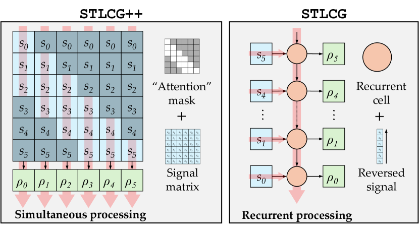
Figure 1: We propose STLCG++  a masking approach to evaluating and backpropagating through signal temporal logic (STL) robustness formulas. The masking approach offers stronger computational, theoretical, and practical benefits compared to STLCG, a recurrent approach.

To construct the computation graph for any STL robustness formula, STLCG processes the time-series input recurrently (see Fig. 1 right), primarily inspired by how recurrent neural networks (RNNs) [17] process sequential data. While consistent with the semantics of STL robustness, recurrent processing leads to the forward and backward passes being comparatively slower than other non-recurrent operations—a widely observed drawback of RNNs. These sequential operations limit STLCG’s capability for efficiently handling long sequence lengths in offline and online settings, especially when combined with other demanding computations, e.g., running foundation models. More recently, attention-based neural architectures, i.e., transformers [18], have demonstrated superior performance in processing sequential data. The key to the transformer architecture is the self-attention operation which operates on all values in the input sequence simultaneously rather than recurrently.

Inspired by the masking mechanism in transformer architectures, we present STLCG++, a masking approach to evaluate and backpropagate through STL robustness for long sequences more efficiently than STLCG, a recurrent-based approach (see Fig. 1 left). STLCG++ opens new possibilities for using STL requirements in long-sequence contexts, especially for online computations, paving the way for further advancements in spatio-temporal behavior generation, control synthesis, and analysis for robotic applications.

Contributions. The contributions of this paper are four-fold. (i) We present STLCG++, a masking-based approach to computing STL robustness, and demonstrate the theoretical, computation, and practical benefits over STLCG, a recurrent-based approach. (ii) We introduce a smoothing function on the time interval of temporal operators and, with the proposed masking approach, enable the differentiability of STL robustness values with respect to time interval parameters. To the best of the authors’ knowledge, this is the first application of differentiating with respect to time parameters within computation graph-based frameworks. (iii) We demonstrate the benefits of our proposed masking approaches with several robotics-related problems ranging from unsupervised learning, trajectory planning, and deep generative modeling. (iv) We provide two open-source STLCG++ libraries, one in JAX and another in PyTorch, and demonstrate their usage via the examples studied in this paper. JAX and PyTorch are well-supported Python libraries used extensively by the deep learning and optimization communities.

II Related work

As STL has been used for various applications, a variety of STL libraries across different programming languages have been developed, including Python, C++, Rust, and Matlab. Given Python is commonly used for robotics research, Tab. I compares recent STL Python packages, particularly capabilities regarding automatic differentiation (AD), vectorization, and GPU compatibility. The libraries generally offer evaluation capabilities of a single signal and their design is tailored towards a specific use case, making it difficult to extend or apply to new settings. If users want to perform an optimization utilizing STL robustness formulas, they must integrate with a separate optimization package (e.g., CVXPY [19], Drake [20]), which may not be straightforward.

RTAMT [21] was introduced as a unified tool for offline and online STL monitoring with an efficient C++ backend. It has received widespread support and has superseded other alternatives in terms of usage. However, RTAMT performs CPU-based signal evaluation and lacks differentiation and vectorization capabilities. This limits its efficiency in handling and optimizing over large datasets, where AD and GPU compatibility are crucial. STLCG was the first to introduce parallelized STL evaluation and backpropagation by leveraging modern AD libraries. However, STLCG faced scalability challenges due to its underlying recurrent computation. STLCG++ addresses these scalability limitations by removing the recurrent operations and making more efficient use of GPUs. We provide two STLCG++ libraries using JAX and PyTorch, which are widely used and well-supported AD/deep learning libraries. The libraries stljax and stlcg-plus-plus can be found at https://github.com/UW-CTRL.

TABLE I: Summary of existing python-based STL toolboxes that are publicly available.

Name	AutoDiff	Vectorize	GPU
STLCG++ (Ours)	JAX, PyTorch	✓	✓
STLCG[8]	PyTorch	✓	✓
Argus [22]	✗	✗	✗
stlpy [23]	✗	✗	✗
PyTeLo [24]	✗	✗	✗
pySTL [25]	✗	✗	✗
RTAMT [21]	✗	✗	✗

III Preliminaries

We provide a brief introduction to STL and related terminologies. See [8, 1] for a more in-depth description.

III-A Signals and trajectories

Signals and subsignals. STL formulas are interpreted over one-dimensional signals $\mathbf{s}=(s_{0},\ldots,s_{T})$, a sequence of scalars sampled at uniform timesteps $\Delta t$ (i.e., continuous-time outputs sampled at finite time intervals) from any system of interest. Given a signal $\mathbf{s}=(s_{0},\ldots,s_{T})$, a subsignal is a contiguous fragment of a signal. By default, we assume a subsignal will start at timestep $t$ and end at the last timestep $T$. We denote such a subsignal by $\mathbf{s}_{t}=(s_{t},\ldots,s_{T})$. If a subsignal ends at a different timestep from $T$, we denote it by $\mathbf{s}_{t}^{K}=(s_{t},\ldots,s_{K})$. Note: The absence of a sub(super)script on $\mathbf{s}$ implies that the signal starts (ends) at timestep 0 ($T$).

States, trajectories, and subtrajectories. Given a system of interest, let $x_{t}\in\mathbb{R}^{n}$ denote the state at timestep $t$. Let $\mathbf{x}=(x_{0},\ldots,x_{T})$ denote a sequence of states sampled at uniform time steps $\Delta t$. Similar to how subsignals are defined, we denote a subtrajectory by $\mathbf{x}_{t}=(x_{t},\ldots,x_{T})$

From trajectories to signals. In this work, we focus specifically on signals computed from a robot’s trajectory. As we will see in the next section, core to any STL formula are predicates which are functions mapping state to a scalar value, $\mu:\mathbb{R}^{n}\rightarrow\mathbb{R}$, with $s_{t}=\mu(x_{t})$, $t=0,\dots,T$. A signal can represent, for example, a robot’s forward speed.

III-B Signal Temporal Logic: Syntax and Semantics

STL formulas are defined recursively according to the following grammar [26, 1],

TruePredicateNotAndUntil.\centering\begin{tabular}[]{cc|c|c|c|c}$\phi::=$&$\top$&$\mu_{c}$&$\neg\phi$&$\phi\wedge\psi$&$\phi\,\mathcal{U}_{[a,b]}\,\psi$\\ &True&Predicate&Not&And&Until\end{tabular}.\@add@centering

:ϕ:=⊤μc¬ϕ∧ϕψϕU[a,b]ψ (1)

The grammar (1) describes a set of recursive operations that, when combined, can create a more complex formula. The time interval $[a,b]$ refers to timesteps rather than specific time values. When the time interval is dropped in the temporal operators, it defaults to the entire length of the input signal. Other commonly used logical connectives and temporal operators can be derived as follows: Or ($\phi\vee\psi:=\neg(\neg\phi\wedge\neg\psi)$), Eventually ($\lozenge_{[a,b]}~\phi:=\top~\mathcal{U}_{[a,b]}~\phi$) and Always ($\square_{[a,b]}~\phi:=\neg F_{[a,b]}~\neg\phi$).

A predicate $\mu_{c}:\mathbb{R}^{n}\rightarrow\mathbb{R}$ is a function that takes, for example, a robot state and outputs a scalar (e.g., speed). Then, given a state trajectory $\mathbf{x}=(x_{0},\ldots,x_{T}),\ x_{t}\in\mathbb{R}^{n}$, we use the notation $\mathbf{x}\models\phi$ to denote that the trajectory $\mathbf{x}$ satisfies $\phi$ according to the Boolean semantics (2).

STL also admits a notion of robustness—the quantitative semantics in (3) describes how much a signal satisfies or violates a formula. Positive robustness values indicate satisfaction, while negative robustness values indicate violation.

III-C Smooth $\max/\min$ approximation

It is often desirable to use STL robustness within gradient-based optimization (e.g., training deep neural networks or trajectory optimization). Since the robustness formulas consist of nested $\max/\min$ operations, smooth approximations $\widetilde{\max}/\widetilde{\min}$ are often used to help with numerical stability. Two typical smooth approximations are $\mathrm{logsumexp}$ and $\mathrm{softmax}$. The smoothness can be controlled by a temperature parameter $\tau$; as $\tau\rightarrow\infty$, the smooth approximations approach to true $\max/\min$ value.

$$\widetilde{\max}_{\mathrm{soft}}(\mathbf{x}) =\sum_{i=1}^{N}x_{i}\frac{\exp^{\tau x_{i}}}{\sum_{i=j}^{N}\exp(\tau x_{j})},$$

$$\widetilde{\max}_{\mathrm{LSE}}(\mathbf{x}) =\frac{1}{\tau}\log\sum_{i=1}^{N}\exp(\tau x_{i}),\>\widetilde{\min}(\mathbf{x})=-\widetilde{\max}(-\mathbf{x})$$

III-D Robustness trace

As STL formulas are made up of nested operations, evaluating the robustness value of the temporal operators (Eventually, Always, and Until), requires the robustness value for each subtrajectory for each subformula. For instance, consider $\lozenge\phi$ where $\phi$ is the subformula. Evaluating $\rho(\mathbf{x},\lozenge\phi)$ requires the robustness value of $\phi$ for all subtrajectories of $\mathbf{x}$, $\rho(\mathbf{x}_{t},\phi)$ for all $t$. Suppose that $\phi$ is another temporal formula, e.g., $\square\varphi$, then we would also require the robustness value of $\varphi$ for all subtrajectories of $\mathbf{x}$. Subsequently, we require the concept of a robustness trace.

Definition 1 (Robustness trace)

Given a trajectory $\mathbf{x}=(x_{0},\ldots,x_{T})$ and an STL formula $\phi$, the robustness trace $\boldsymbol{\tau}(\mathbf{x},\phi)$ is a sequence of robustness values of $\phi$ for each subtrajectory of $\mathbf{x}$. That is,

$$\boldsymbol{\tau}(\mathbf{x},\phi)=\rho(\mathbf{x}_{0},\phi),\,\rho(\mathbf{x}_{1},\phi),\ldots,\rho(\mathbf{x}_{T},\phi).$$ (4)

Computing the robustness trace of non-temporal operations is straightforward as there is no need to loop through time, and we omit that description in this paper.

III-E Recursive structure of STL formulas

To compute the robustness value of any STL formula $\phi$ with arbitrary formula depth, we must first calculate the robustness trace of its subformulas. However, each subformula’s robustness trace depends on the robustness traces of its subformulas, and this dependency continues recursively since STL formulas are constructed by repeatedly applying STL operators on top of each other. Fig. 2 illustrates how the trajectories are passed through each operation of an STL formula to compute the robustness trace of each subformula.

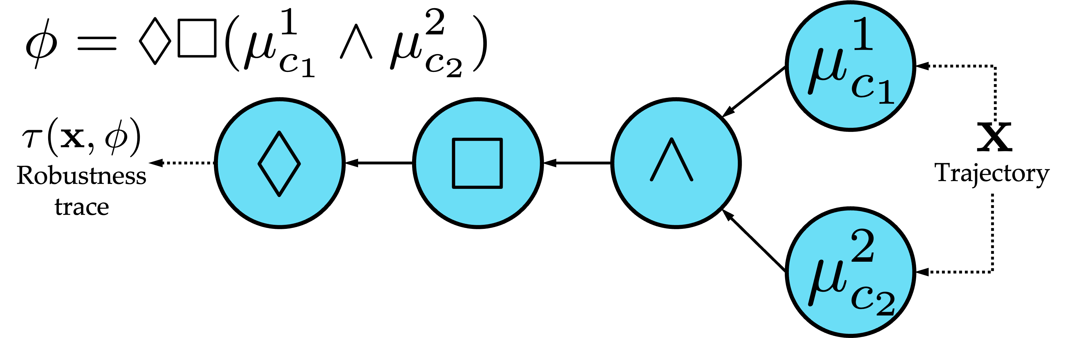
Figure 2: Example illustration of the graph structure of an STL formula. Input trajectories are passed through the predicates (inner most nodes) passed through the graph towards the last (outer most) STL operator.

III-F STLCG: Recurrent computation

We briefly outline the recurrent operations underlying STLCG; for more details, we refer the reader to [8]. Illustrated in Fig. 1 (right), STLCG utilizes the concept of dynamic programming to calculate the robustness trace. The input signal is processed backward in time, and a hidden state is maintained to store the information necessary for each recurrent operation at each time step. The choice of recurrent operation depends on the temporal STL formula (either a $\max$ or $\min$). The size of the hidden state depends on the time interval of the temporal operator and is, at most, the length of the signal. Although the use of a hidden state to summarize past information helps reduce space complexity, the recurrent operation leads to slow evaluation and backpropagation due to sequential dependencies. Next, we present a masking-based approach that bypasses the sequential dependency, leading to faster computation times.

IV Masking approach for temporal operations

We propose STLCG++, a masking approach to compute STL robustness traces. Fig. 1 illustrates the masking approach, highlighting the idea that each value of a robustness trace is computed simultaneously, rather than sequentially, as we saw with STLCG. Mirroring the concept of attention masks in transformer architectures [18], we introduce a mask $M$ to select relevant parts of a signal that can be later processed simultaneously rather than sequentially. In the rest of this section, we describe the masking operation underpinning STLCG++ and several properties.

IV-A Notation and masking operation

Before dive into the details, we first introduce some notation. We assume we have as input (1D) signal $\mathbf{s}$ of length $T+1$, and let $K$ denote the number of time steps contained (inclusive) in the time interval $[a,b]$ given an STL temporal operator. A mask $\mathcal{M}$ is an $n-$dimensional array whose entries are wither $1$ or $0$. A mask $\mathcal{M}$ is applied via element-wise multiplication to an array $\mathcal{S}$ of the same size. For entries $(i,j)$ where $\mathcal{M}_{ij}=0$, the corresponding entries $\mathcal{S}_{ij}$ will be ignored, or is masked out. We can replace the entries that are masked out with an arbitrary value, typically a large positive or negative value. Let $\mathcal{M}\odot_{\pm}\mathcal{S}$ denote the application of mask $\mathcal{M}$ on $\mathcal{S}$ and masked out by either a large positive or negative number.

IV-B Eventually and Always operations

For brevity, we describe the procedure for the Eventually operation but note that the procedure for the Always operation is almost identical except a $\min$ operation is used instead of $\max$. Consider the formula $\psi=\lozenge_{[a,b]}\phi$, and let $\mathbf{s}=\boldsymbol{\tau}(\mathbf{x},\phi)$ denote the robustness trace of $\phi$. Specifically, $s_{t}=\rho(\mathbf{x}_{t},\phi)$. Then, we seek to find the robustness trace,

$$\boldsymbol{\tau}(\mathbf{x},\lozenge_{[a,b]}\phi)=\biggl{\{}\max_{i\in[a,b]}s_{t+i}\biggl{\}}_{t=0}^{T}$$

Intuitively, we want to slide a time window $[a,b]$ along $\mathbf{s}$ and take the $\max$ of the values within the window. Rather than performing this set of operations sequentially, we first “unroll” the sequential operation—turning the 1D signal into a 2D array, second, we apply a 2D mask to mask out the irrelevant entries dictated by the time window, and third, we use the $\max$ operation over the unmasked values.

Step 1:“Unrolling” the signal. First, we pad the end of the signal by the size of the time window $K$; the reason will be apparent in Step 3. The padding value $\bar{s}$ can be set by the user, such as extending the last value of the signal, or setting it to a large negative number. Then, we turn the padded signal into a 2D array $\mathcal{S}$ by repeating the signal along the second dimension $T$ times, resulting in a $(T+K)\times K$ 2D array. An example is provided in (5).

Step 2: Construct 2D mask. We construct a mask $\mathcal{M}$ that will be applied to the unrolled signal $\mathcal{S}$. The mask $\mathcal{M}$ comprises two sub-masks: (i) subsignal mask $\mathcal{M}_{\mathrm{subsig}}$ and (ii) time interval mask $\mathcal{M}_{\mathrm{time}}$.

Subsignal mask $\mathcal{M}_{\mathrm{subsig}}$: This mask incrementally masks out the start of the signal as we move along the horizontal (second) dimension of $\mathcal{S}$. $\mathcal{M}_{\mathrm{subsig}}$ is upper triangular with an offset of one to exclude the diagonal entries. After applying the $\mathcal{M}_{\mathrm{subsig}}$ on $\mathcal{S}$, the columns of the unmasked entries correspond to all the subsignals of $\mathbf{s}$. An example $\mathcal{M}_{\mathrm{subsig}}$ is illustrated by the red shaded entries in (5).

Time interval mask $\mathcal{M}_{\mathrm{time}}$: This mask masks out all the entries outside of time interval $[a,b]$ for each subsignal. $\mathcal{M}_{\mathrm{time}}$ consists of an off-diagonal strip that masks out entries before the start of the interval (determined by $a$), and a lower triangular matrix with an offset that masks out entries after the interval (determined by $b$). An example is illustrated by the blue shaded entries in (5).

Final mask $\mathcal{M}$: The final mask is $\mathcal{M}=\mathcal{M}_{\mathrm{subsig}}+\mathcal{M}_{\mathrm{time}}$, resulting in a mask that retains all the entries within the time interval $[a,b]$ for each sub-signal.

Step 3: Apply 2D mask and $\max$ operation. Given $\mathcal{S}$ and $\mathcal{M}$ from the previous steps, we can compute $\mathcal{M}\odot_{-}\mathcal{S}$, similar to what is done in the mask attention mechanism in transformer architectures. Then, we apply the $\max$ operation along each column. Note the padding we did back in step 1 becomes relevant when the time interval exceeds the length of the subsignal. This is similar to the approach taken in [8] to handle incomplete signals. For the Always operation, $\min$ and $\mathcal{M}\odot_{+}\mathcal{S}$ are used instead.

Example 1

Consider the STL formula $\psi=\lozenge_{[1,3]}(s>0)$ and a signal with 8 time steps, $\mathbf{s}=[s_{0},\ldots,s_{7}]$. The corresponding unrolled 2D array is shown (5) with padding value $\bar{s}$, and the red shaded entries denote the entries masked out by the subsignal mask. The blue shaded entries denote the entries masked out by the time interval mask.

$${\small\bNiceMatrix[margin]\Block[fill=blue!15,rounded-corners]{1-1}{}s_{0}&\Block[fill=red!15,rounded-corners]{1-7}{}s_{0}s_{0}s_{0}s_{0}s_{0}s_{0}s_{0}\\ s_{1}\Block[fill=blue!15,rounded-corners]{1-1}{}s_{1}\Block[fill=red!15,rounded-corners]{1-6}{}s_{1}s_{1}s_{1}s_{1}s_{1}s_{1}\\ s_{2}s_{2}\Block[fill=blue!15,rounded-corners]{1-1}{}s_{2}\Block[fill=red!15,rounded-corners]{1-5}{}s_{2}s_{2}s_{2}s_{2}s_{2}\\ s_{3}s_{3}s_{3}\Block[fill=blue!15,rounded-corners]{1-1}{}s_{3}\Block[fill=red!15,rounded-corners]{1-4}{}s_{3}s_{3}s_{3}s_{3}\\ \Block[fill=blue!15,rounded-corners]{1-1}{}s_{4}s_{4}s_{4}s_{4}\Block[fill=blue!15,rounded-corners]{1-1}{}s_{4}\Block[fill=red!15,rounded-corners]{1-3}{}s_{4}s_{4}s_{4}\\ \Block[fill=blue!15,rounded-corners]{1-2}{}s_{5}s_{5}s_{5}s_{5}s_{5}\Block[fill=blue!15,rounded-corners]{1-1}{}s_{5}\Block[fill=red!15,rounded-corners]{1-2}{}s_{5}s_{5}\\ \Block[fill=blue!15,rounded-corners]{1-3}{}s_{6}s_{6}s_{6}s_{6}s_{6}s_{6}\Block[fill=blue!15,rounded-corners]{1-1}{}s_{6}\Block[fill=red!15,rounded-corners]{1-1}{}s_{6}\\ \Block[fill=blue!15,rounded-corners]{1-4}{}s_{7}s_{7}s_{7}s_{7}s_{7}s_{7}s_{7}\Block[fill=blue!15,rounded-corners]{1-1}{}s_{7}\\ \Block[fill=blue!15,rounded-corners]{1-5}{}\bar{s}\bar{s}\bar{s}\bar{s}\bar{s}\bar{s}\bar{s}\bar{s}\\ \Block[fill=blue!15,rounded-corners]{1-6}{}\bar{s}\bar{s}\bar{s}\bar{s}\bar{s}\bar{s}\bar{s}\bar{s}\\ \Block[fill=blue!15,rounded-corners]{1-7}{}\bar{s}\bar{s}\bar{s}\bar{s}\bar{s}\bar{s}\bar{s}\bar{s}\\ }$$ (5)

After filling the masked entries with a large negative value, and taking the $\max$ column-wise. Let $\mathbf{s}=[0,1,2,3,4,5,6,7]$ and $\bar{s}=7$ (this extends the last value of the signal past the signal length), then the robustness trace is $\tau(\mathbf{s},\psi)=[3,4,5,6,7,7,7,7]$. If we set $\bar{s}=-\infty$ (we do not consider extending the signal past the signal length), then the robustness trace is $\tau(\mathbf{s},\psi)=[3,4,5,6,7,-\infty,-\infty,-\infty]$.

IV-C Until operation

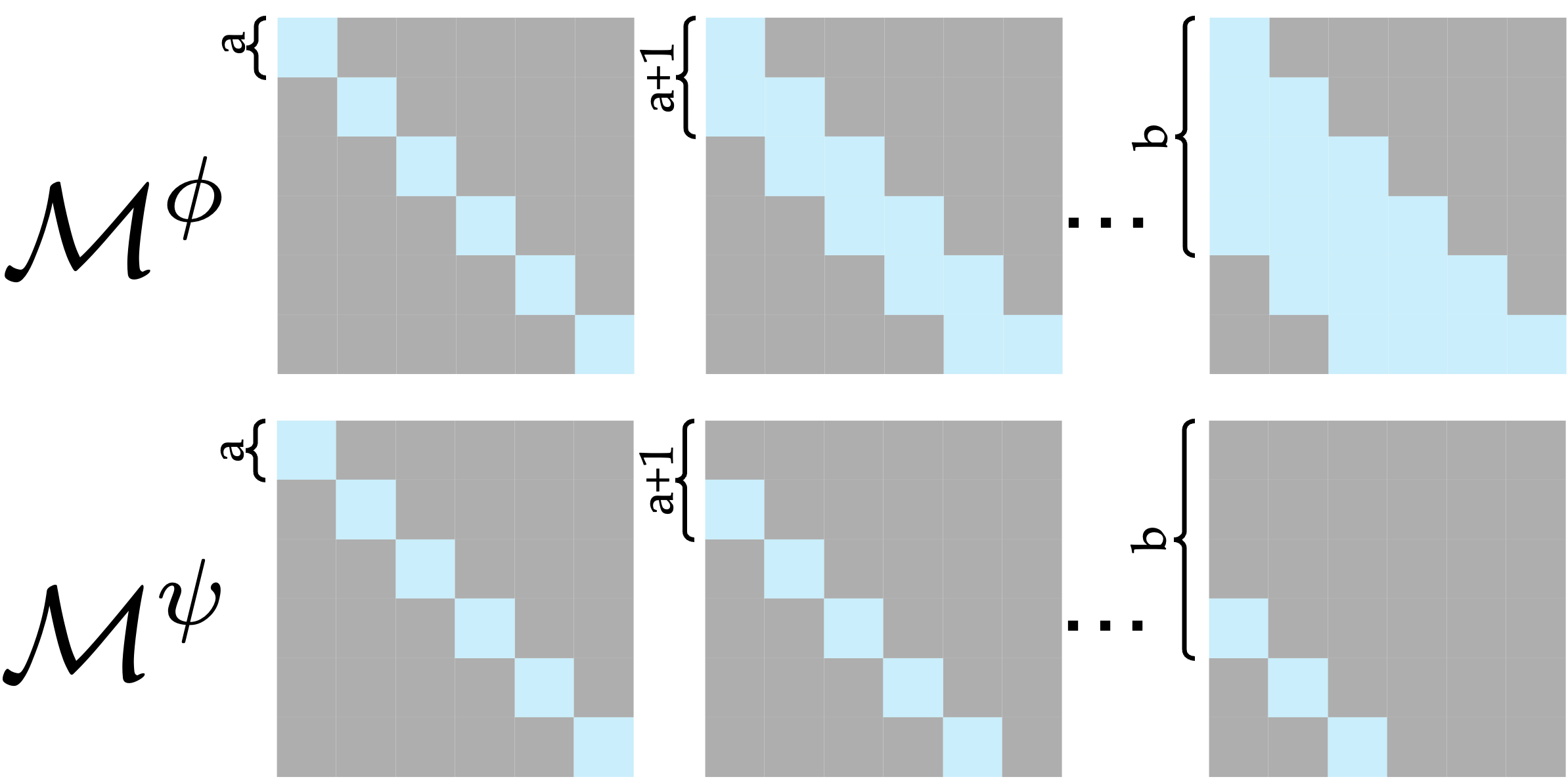
Figure 3: Illustration of the slices that make up $\mathcal{S}^{\phi}$ and $\mathcal{S}^{\psi}$ for the Until formula $\phi\ \mathcal{U}_{[a,b]}\psi$. In this figure, $a=0$.

We can apply a similar masking strategy for the Until operation, following a similar three-step process described in Sec. IV-B. The main differences are (i) the signal needs to be “unrolled” into three dimensions, and (ii) the operations in Step 3 correspond to the Until robustness formula.

Consider the formula $\phi\,\mathcal{U}_{[a,b]}\psi$. Let $\mathbf{s}^{\phi}=\boldsymbol{\tau}(\mathbf{x},\phi)$ and $\mathbf{s}^{\psi}=\boldsymbol{\tau}(\mathbf{x},\psi)$ denote the robustness trace of $\phi$ and $\psi$ respectively for trajectory $\mathbf{x}$. Specifically, $s_{t}^{\phi}=\rho(\mathbf{x}_{t},\phi)$ and $s_{t}^{\psi}=\rho(\mathbf{x}_{t},\psi)$. Then, we seek to find the robustness trace,

$$\boldsymbol{\tau}(\mathbf{x},\phi\,\mathcal{U}_{[a,b]}\psi)=\Bigg{\{}\max_{i\in[a,b]}\bigg{\{}\min\left(\min_{\tau\in[0,i]}s_{t+\tau}^{\phi},\ s_{t+i}^{\psi})\right)\bigg{\}}\Bigg{\}}_{t=0}^{T}$$

Step 1:“Unrolling” the signal. Given a signal $\mathbf{s}$, we construct a 3D array by repeating the signal along the first and second dimensions, resulting in a $T\times T\times K$ array. This unrolling operation on $\mathbf{s}^{\phi}$ and $\mathbf{s}^{\psi}$ results in $\mathcal{S}^{\phi}$ and $\mathcal{S}^{\psi}$.

Step 2: Construct 3D mask. In the Until robustness formula, we need to evaluate $\min_{\tau\in[0,i]}\mathbf{s}_{t+\tau}^{\phi}$ and $\mathbf{s}_{t+i}^{\psi}$ for $i\in[a,b]$ and for all $t$. For a given $i$, notice that $\rho(\mathbf{x}_{t},\square_{[0,i]}\phi)=\min_{\tau\in[0,i]}\mathbf{s}_{t+\tau}^{\phi}$ and $\rho(\mathbf{x}_{t},\square_{[i,i]}\psi)=\mathbf{s}_{t+i}^{\psi}$ which is something we can compute given the procedure outlined in Sec. IV-B. However, the outer $\max$ requires us to consider all $i\in[a,b]$. Thus for each formula $\square_{[0,i]}\phi$ and $\square_{[i,i]}\psi$, we stack all the 2D masks for each value of $i\in[a,b]$ across the third dimension, resulting in two 3D masks, $\mathcal{M}^{\phi}$ and $\mathcal{M}^{\psi}$. A visualization is shown in Fig. 3.

Step 3: Apply the Until robustness formula operations. We can now apply all the operations needed to compute the robustness trace for the Until operation. After Step 2, we have $\mathcal{S}^{\phi}$, $\mathcal{S}^{\psi}$, and the 3D masks $\mathcal{M}^{\phi}$ and $\mathcal{M}^{\psi}$. We can compute $\mathcal{M}^{\phi}(\mathcal{S}^{\phi},\infty)$ and $\mathcal{M}^{\psi}(\mathcal{S}^{\psi},\infty)$. Then, we can apply the following set of operations.

$$S_{1} =\overbrace{\underset{\mathrm{dim}=1}{\mathrm{stack}}\left(\left[\min_{\mathrm{dim}=1}\mathcal{M}^{\phi}(\mathcal{S}^{\phi},\infty),\min_{\mathrm{dim}=1}\mathcal{M}^{\psi}(\mathcal{S}^{\psi},\infty)\right]\right)}^{\text{Size }[2\times T\times K]}$$

$$S_{2} =\min_{\mathrm{dim}=1}S_{1},\qquad(S_{2}\text{ has size }[T\times K])$$

$$S_{3} =\max_{\mathrm{dim}=2}S_{2},\qquad(S_{3}\text{ has size }[T])$$

We see that this set of operations is relatively simple, a series of $\min$ and $\max$ operations along various dimensions, and these operations remain the same regardless of the choice of time intervals, unlike the recurrent approach.

IV-D Dependence on smooth approximations

In this section, we show the choice of $\max/\min$ approximation with the recurrent operations leads to incorrect gradient attribution, whereas the masking approach does not.

Both masking and recurrent approaches output the correct robustness values when the true $\min/\max$ operations and $\mathrm{logsumexp}$ approximation are used. However, if the $\mathrm{softmax}/\mathrm{softmin}$ approximation is used with a recurrent approach, the output robustness values and gradient values do not correctly reflect the correct $\max/\min$ value. This is because, when applying $\mathrm{softmin}/\mathrm{softmax}$ in a recurrent fashion, values applied earlier in the recurrence will be “softened” more than values applied later in the recurrence, even if they are the true $\max$ or $\min$ value. Not only does nesting the $\mathrm{softmin}/\mathrm{softmax}$ operations give a very poor approximation of the true $\min/\max$ value, but it also artificially increases the gradient for values passed later in the recurrence. Whereas with the $\mathrm{logsumexp}$ approximation, applying it recursively over multiple values is the same as applying it once over all the values. That is, $\widetilde{\max}_{\mathrm{LSE}}([\widetilde{\max}_{\mathrm{LSE}}(\mathbf{x}),y])=\widetilde{\max}_{\mathrm{LSE}}([\mathbf{x},y])$ where as $\widetilde{\max}_{\mathrm{soft}}([\widetilde{\max}_{\mathrm{soft}}(\mathbf{x}),y])\neq\widetilde{\max}_{\mathrm{soft}}([\mathbf{x},y])$. This issue is not observed when using the masking-based approach due to the way subsignals are processed without recurrence as highlighted in earlier sections.

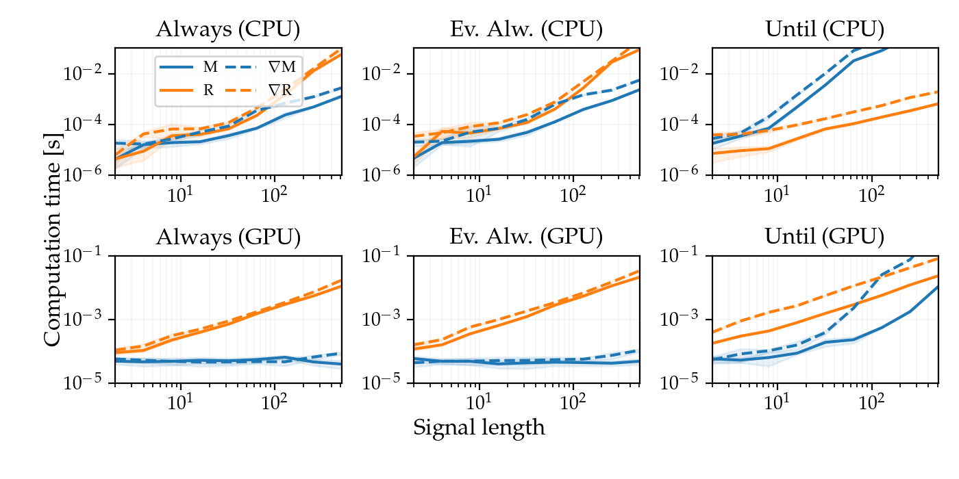
(a) Computation time using JAX with JIT compilation.

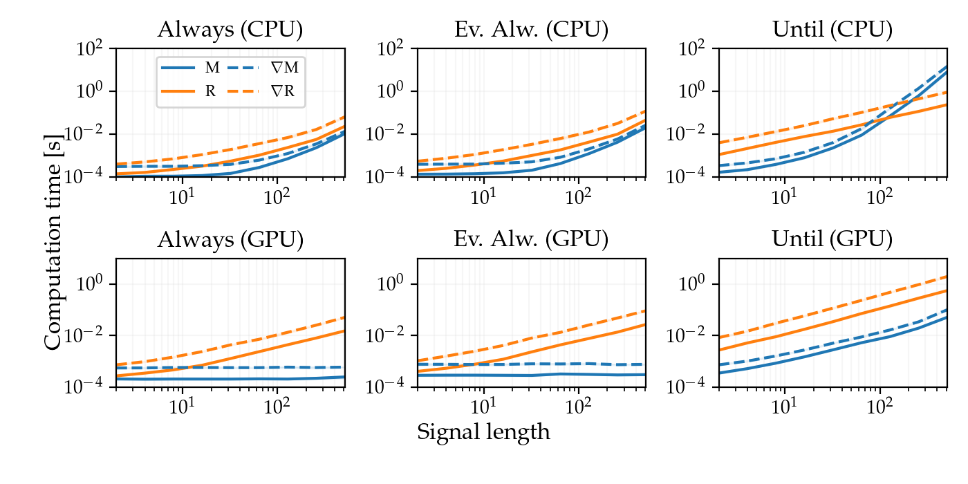
(b) Computation time using PyTorch.

Figure 4: Comparison of computation time for masking and recurrent approach on CPU and GPU as signal length increases. Results were tested on formulas (Always) $\square(\phi\wedge\psi)$, (Ev. Alw.) $\lozenge\square(\phi\wedge\psi)$, and (Until) $\phi\ \mathcal{U}\ \psi$.

IV-E Practical benefits

In terms of practical benefits, the masking approach is relatively easier to use compared to the recurrent approach. We highlight several reasons why this is the case. (i) Software design. The recurrent approach required signals to be passed backward in time. This increased the complexity of software design and was not often intuitive for end users. With the masking approach, there is no need to reverse the signal. (ii) Static graph structure. With the recurrent approach, the choice of time interval would fundamentally change the dimension of hidden states, whereas the graph structure remains the same for the masking approach. Keeping the same graph structure even if the intervals change is essential in compilation. (iii) Vectorization and just-in-time compilation. Related to the second point above, the static graph structure afforded by the masking approach enables the ability to easily vectorize and just-in-time compile (JIT) the computation over not just various signal inputs but also various time intervals. The ability to vectorize and JIT over different time intervals can be particularly useful in formula mining applications where we may want to simultaneously evaluate robustness formulas with different time intervals. (iv) Conformity to popular deep learning libraries. By leveraging AD libraries that power popular deep learning frameworks (e.g., JAX and PyTorch), STLCG++ becomes more accessible to the broader community and seamlessly integrates into the ecosystem.

V Computational properties of STLCG++

In this section, we analyze the computational properties of the approaches STLCG++ (masking-based) and STLCG (recurrent-based) by measuring the computation time required to compute robustness values and their gradient. We seek to answer the following research questions.

RQ1: Does STLCG++ compute robustness traces faster than STLCG as measured by median computation time?

RQ2: How does STLCG++’s computation time scale with sequence length compared to STLCG?

We test on three different patterns of (temporal) STL formulas: $\phi_{1}=\square(\phi\wedge\psi)$ (single temporal operator), $\phi_{2}=\lozenge\square(\phi\wedge\psi)$ (two nested temporal operators), and $\phi_{3}=\phi\,\mathcal{U}\psi$ (the until operator), where $\phi$ and $\psi$ are simple predicates. These formulas were chosen as representatives of commonly encountered patterns in practice, as highlighted in [27].

We evaluate computation time for increasing signal lengths up to $T=512$ time steps with a batch size of $8$. For context, trajectory lengths from robotics-related trajectory optimization problems are typically $\leq 50$. We also consider both CPU and GPU backends. We present our results in Fig. 4 and Table II using JAX with JIT compilation (JAX+JIT) and PyTorch and make the following observations.

V-A Evaluation with CPU backend

RQ1. We observe that the masking approach achieves lower (median) computation times compared to the recurrent approach for both $\phi_{1}$ and $\phi_{2}$. This trend is observed for both JAX+JIT and Pytorch. The masking-based approach performs worse than the recurrent-based approach for $\phi_{3}$ for JAX+JIT but performs better for Pytorch. We believe that this difference is observed due to how each library manages and allocates memory on CPU.

RQ2. As expected, the computation time for both masking and recurrent approaches increases with the input length. However, while the time of the recurrent approach grows linearly due to its sequential processing, masking exhibits a slower increase in computation time for $\phi_{1}$ and $\phi_{2}$. This makes masking more suitable for handling long sequence lengths for those formulas. However, for $\phi_{3}$ we observe that the masking approach performs significantly worse on JAX but outperforms on PyTorch for signal lengths $\leq$ 128.

V-B Evaluation with GPU backend

RQ1. The masking approach performs significantly faster than the recurrent approach when using the GPU, for all test cases. This difference is statistically significant ($p<0.001$), indicating a clear advantage of the masking approach over the recurrent approach when using GPU.

RQ2. The computation time for both masking and recurrent approaches increases with sequence length. For $\phi_{1}$ and $\phi_{2}$ the recurrent approach scales linearly with a steep growth rate, while the masking approach remains nearly constant, demonstrating superior efficiency on GPU. For $\phi_{3}$, both approaches exhibit linear scaling.

V-C Summary discussion

We observe that across all backends, AD libraries, and sequence lengths, masking outperforms the recurrent-based approach for formulas such as $\phi_{1}$ and $\phi_{2}$. As highlighted in [27], these formulas pattern occur the most in surveyed literature and are used extensively for various applications. For formulas with the Until operator, we observe that the choice of approach depends on the backend. For GPU backends, the masking-based approach is preferred over the recurrent approach. However, for the CPU backend, the masking approach performs worse as the 3D signal masking incurs significant memory costs.

TABLE II: Relative computation time of masking approach compared to recurrent approach. Median value across different signal lengths. Lower is better.

Device	CPU	GPU	CPU	GPU
Formula	JAX + JIT		Pytorch
$\square(\phi\wedge\psi)$	$-37.99\%$	$-93.43\%$	$-76.05\%$	$-85.76\%$
$\lozenge\square(\phi\wedge\psi)$	$-51.51\%$	$-96.65$%	$-82.50\%$	$-89.03\%$
$\phi\ \mathcal{U}\ \psi$	$822.01\%$	$-91.31\%$	$-88.22\%$	$-94.15\%$

VI Smoothing time intervals

By using the masking operation to capture parts of the signal within the specified time interval, we can build a smooth approximation of the mask and differentiate robustness values with respect to the parameters of the mask that determine which values are selected. As such, it becomes possible to perform gradient descent over time interval parameters to find, for example, a time interval that best explains time-series data. We showcase two examples in Sec. VII utilizing this new capability. Notably, this differentiation was not possible with STLCG since the choice of time intervals impacted the size of the hidden state used within the recurrent computations, thus making the robustness value non-differentiable with respect to time interval bounds.

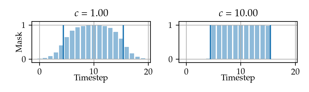
Figure 5: Illustration of the smooth mask for various values of smoothing parameter $c$.

Rather than using a mask with $0$ and $1$’s as described in Sec. IV-B and IV-C, we use the following smooth mask approximation. For a sequence length of $T$, we have,

$$\widetilde{\mathrm{mask}}(i;a,b,c,\epsilon)=\max(\sigma(c(i-aT))-\sigma(c(i-bT))-\epsilon,0),$$ (6)

where $i$ is the time index, $\sigma(x)$ is the sigmoid function, the parameters $0\leq a<b\leq 1$ denote the fraction along the signal of the start and end of the time interval, $c$ denotes the mask smoothing parameter, and $\epsilon$ denotes a user-defined tolerance. Fig. 5 shows a visualization of the smooth mask and how the smoothing parameter $c$ affects the mask.

When optimizing over time interval parameters, we can anneal the smooth mask parameter $c$ to help with convergence to a (local) optima on a generally nonlinear loss landscape (see Sec. VII-C for more details). As noted before, a benefit of the masking approach is that the operations can be easily vectorized. We can simultaneously evaluate the robustness for multiple time intervals and perform gradient descent on multiple values. As such, we can envision a use case where we perform a coarse global search via sampling and then a local refinement via gradient descent.

For reference, using the vectorized mapping function in JAX+JIT, the computation time to evaluate $90,000$ different values for $(a,b)$ with a signal of length $T=20$ for the formula $\square_{[aT,bT]}(s>0)$ is $1.87\pm 0.0164$ms on a M2 MacBookPro. This averages to around $20.78\mu$s per time interval value. In contrast, (sequentially) searching over all possible valid time intervals for a signal length of 20 (i.e., 190 intervals with integer interval limits) using the recurrent approach takes about $5.25\pm 0.0497$s, or roughly $27.6$ms each evaluation. This means that STLCG++ offers more than 1000$\boldsymbol{\times}$ improvement in computation time when evaluating STL robustness over multiple time interval values.

VII Robotics-related applications

We showcase a variety of use cases that demonstrate the computational advantages of the masking approach. We provide two Python STLCG++libraries, one in JAX [28] and another in PyTorch [29]. We discuss how STLCG++ opens up new possibilities for robot planning and control.

VII-A Trajectory planning with suboptimal STL specifications.

Trajectory optimization is essential in robotic systems, enabling precise navigation and task execution under complex constraints. These trajectories must balance user-defined goals with feasibility and efficiency. Since goal misspecification can lead to erroneous behavior, infeasibility, or subpar performance, we show how suboptimal goals (captured through STL specifications) can be refined in addition to solving for an optimal trajectory. Consider a trajectory optimization problem where we would like to reach a goal region while visiting a target region within a fixed time horizon. Additionally, the visit duration of is to be maximized. Consider a specification $\phi=\square_{[aT,bT]}(\text{inside }\leavevmode\hbox to12.57pt{\vbox to12.57pt{\text{[drawing]}}})\wedge\lozenge(\text{inside }\leavevmode\hbox to12.57pt{\vbox to12.57pt{\text{[drawing]}}})$ which specifies a time window that the trajectory should be inside . We cast this trajectory planning problem as an unconstrained optimization problem,

$$\min_{\mathbf{u},a,b}\gamma_{1}J_{\mathrm{STL}}(\mathbf{x})+\gamma_{2}J_{\mathrm{I}}(a,b)+\gamma_{3}J_{\mathrm{lim}}(\mathbf{u})+\gamma_{4}J_{\mathrm{eff}}(\mathbf{u}),$$

$$J_{\mathrm{STL}}(\mathbf{x})=\mathrm{ReLU}(-\rho(\mathbf{x},\phi)),\quad J_{\mathrm{I}}(a,b)=\exp(2(\tilde{I}-b+a)),$$

$$J_{\mathrm{lim}}(\mathbf{u})=\frac{1}{T}\sum_{t=0}^{T-1}\mathrm{ReLU}(\|\mathbf{u}_{t}\|_{2}-\bar{u}),\>J_{\mathrm{eff}}(\mathbf{u})=\frac{1}{T}\sum_{t=0}^{T-1}\|\mathbf{u}_{t}\|_{2}^{2},$$

where $\mathbf{x}$ is the state trajectory from executing $\mathbf{u}$ with single integrator discrete-time dynamics. We use a timestep of $\Delta t=0.1$, $T=51$, $\bar{u}=2$ is the system’s maximum control limits, and $\tilde{I}=0.2$ is a nominal (normalized) time interval size that we would like to improve upon. We randomly initialized the control inputs and $(a,b)_{\mathrm{init}}=(0.14,0.82)$. Using coefficients $\gamma_{1}=1.1,\gamma_{2}=0.05,\gamma_{3}=2,\gamma_{4}=0.5$, the resulting solution is shown in Fig. 6(a) with final values $(a,b)_{\mathrm{final}}=(0.37,0.84)$. The final optimized STL formula is $\phi=\square_{[20,43]}(\text{inside }\leavevmode\hbox to12.57pt{\vbox to12.57pt{\text{[drawing]}}})\wedge\lozenge(\text{inside }\leavevmode\hbox to12.57pt{\vbox to12.57pt{\text{[drawing]}}})$. Using JAX, each gradient step took about $92.3\pm 3.99\mu$s on an M2 MacBookPro. With unconstrained multiobjective optimization, selecting objective weights that achieve desirable behavior can be tedious. With STLCG++, we can perform gradient descent computation over various coefficient values simultaneously and then select the best one.

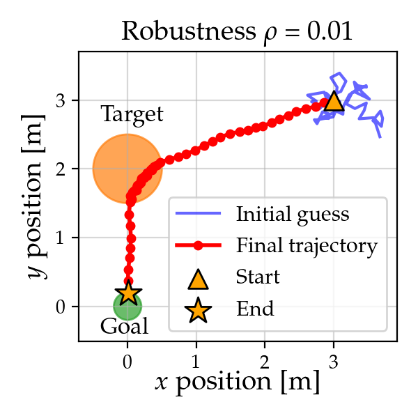
(a) Trajectory with optimized time interval in orange target region.

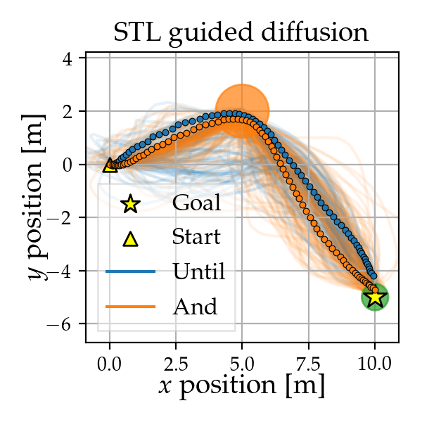
(b) Generated trajectories using STL guided DDIM.

Figure 6: Trajectories generated using STLCG++ with STL robustness in the planning objective.

VII-B Deep generative modeling: STL-guided diffusion policies

We demonstrate the use of STL specifications for guided diffusion models [30, 31], a recent type of deep generative models that present a promising approach for robot policy learning [32, 33] and behavior generation [4]. We build off work from [33] that uses Control Barrier and Lyapunov functions (CBFs and CLFs) to guide the denoising process of a diffusion model for safe control sequence generation. In this application, we use STL robustness in place of CBFs and CLFs as the guidance function. We trained a DDIM model, generating trajectories with 80-time steps. We used 200 denoising steps and a batch size of 128, we generated trajectory samples using two different STL guidance functions,

$$\phi_{\mathcal{U}} =\lozenge\square_{[0,10]}(\text{inside }\leavevmode\hbox to12.57pt{\vbox to12.57pt{\text{[drawing]}}})\ \mathcal{U}\ \lozenge\square_{[0,5]}(\text{inside }\leavevmode\hbox to12.57pt{\vbox to12.57pt{\text{[drawing]}}})$$

$$\phi_{\wedge} =\lozenge\square_{[0,10]}(\text{inside }\leavevmode\hbox to12.57pt{\vbox to12.57pt{\text{[drawing]}}})\wedge\lozenge_{[60,80]}\square_{[0,5]}(\text{inside }\leavevmode\hbox to12.57pt{\vbox to12.57pt{\text{[drawing]}}}).$$

The resulting trajectories are shown in Fig. 6(b). Although guided diffusion does not guarantee that the STL specifications are strictly satisfied, we observe a satisfaction rate of $52.34\%$, $62.50\%$ for $\phi_{\mathcal{U}}$ and $\phi_{\wedge}$, respectively. This shows how STLCG++ can enhance diffusion policies to promote safer behavior generation.

VII-C Machine learning: STL parameter mining from data

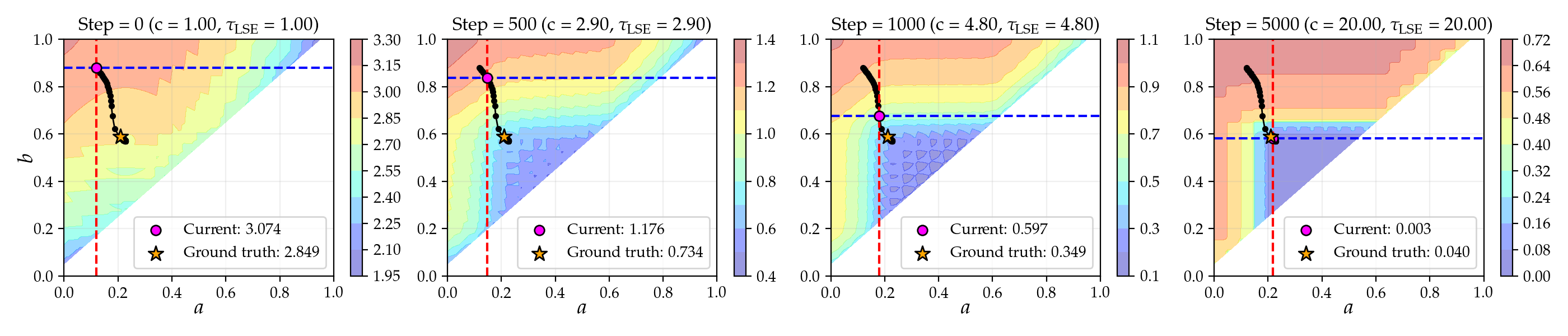
Figure 7: The masking approach enables a smooth approximation of time intervals, enabling the use of gradient descent over time interval parameters. The contour plots show the loss landscape given by (7) as a function of $a,b$, the normalized time interval limits. The solution at gradient descent step 0, 500, 1000, and 5000 are shown. Note that the smooth time mask parameter and approximate $\max/\min$ temperature values are annealed over the steps.

Formal STL specifications are a crucial piece in building robust robot systems, playing a role in controller synthesis [15], fault localization [34], and anomaly detection and resolution [35]. However, specifications are not often readily available, making specification mining from data an important problem to study [36]. In this example, we perform STL specification mining from data. Specifically, we leverage the differentiability and vectorization over smooth time intervals to find a time interval that best fits the observed data. Consider a dataset of (noisy) signals with $T=20$ timesteps. The signals have value $1$ between the normalized time interval of $(a,b)=(0.23,0.59)$ and zero elsewhere. Some noise is added around $(a,b)$ and to the signal itself. The goal is to learn the largest time interval $[\bar{a},\bar{b}]$ such that the signals from the dataset satisfy $\phi=\square_{[\bar{a},\bar{b}]}(s>0)$. We frame this STL mining problem with an optimization problem,

$$\min_{0\leq a<b\leq 1}\>\frac{1}{N}\sum_{\mathbf{s}\in\mathcal{D}}\max(-\rho(\mathbf{s},\square_{[aT,bT]}(s>0)),0)+\gamma(a-b)\vskip-5.69054pt$$ (7)

where $\gamma$ is a coefficient on the term $a-b$ that encourages the interval to be larger. We solve (7) via gradient descent, using the smooth time interval mask discussed in Sec. VI. Specifically, we annealed the time interval mask scaling factor and the temperature with a sigmoid schedule, and performed 5000 gradient steps with a step size of $10^{-2}$. To ensure $0\leq a<b\leq 1$, we passed them through a sigmoid function first. Fig. 7 shows a few snapshots of the gradient steps and the loss landscape as the scaling parameter and temperature increase. We can observe that our solution converges to the global optimum and is consistent with the ground truth values (subject to the injected noise). To give a sense of the computation time, using JAX on a M2 MacbookPro, it took about $122\pm 0.479\mu$s per gradient step.

VIII Conclusion

We have presented STLCG++, a masking-based approach to computing STL robustness leveraging automatic differentiation libraries. STLCG++ mimics the operations that underpin transformer architectures, and we demonstrate the computational, theoretical, and practical benefits of the proposed masking approach over STLCG  which uses a recurrent approach. The observed advantages of masking over recurrent operations mirror the advantages of using transformers over recurrent neural networks for processing sequential data. We also present two STLCG++ libraries in JAX and PyTorch, demonstrating their usage in several robotics-related problems such as machine learning, trajectory planning, and deep generative modeling. STLCG++ offers significant computational advantages over STLCG, thus presenting new exciting opportunities for incorporating STL specifications into various online robot planning and control robot tasks requiring fast computation and inference speeds.

References

- [1] O. Maler and D. Nickovic, “Monitoring temporal properties of continuous signals,” Lecture Notes in Computer Science, no. 3253, pp. 152–166, 2004.
- [2] Y. V. Pant, H. Abbas, and R. Mangharam, “Smooth operator: Control using the smooth robustness of temporal logic,” in IEEE Conf. on Control Technology and Applications, 2017.
- [3] Y. Gilpin, V. Kurtz, and H. Lin, “A smooth robustness measure of signal temporal logic for symbolic control,” IEEE Control Systems Letters, vol. 5, no. 1, pp. 241–246, 2020.
- [4] Y. Meng and C. Fan, “Diverse controllable diffusion policy with signal temporal logic,” IEEE Robotics and Automation Letters, vol. 9, no. 10, pp. 8354–8361, 2024.
- [5] M. Ma, J. Gao, L. Feng, and J. Stankovic, “STLnet: Signal temporal logic enforced multivariate recurrent neural networks,” in Conf. on Neural Information Processing Systems, 2020.
- [6] W. Liu, N. Mehdipour, and C. Belta, “Recurrent neural network controllers for signal temporal logic specifications subject to safety constraints,” IEEE Control Systems Letters, vol. 6, pp. 91 – 96, 2021.
- [7] S. Yaghoubi and G. Fainekos, “Worst-case satisfaction of STL specifications using feedforward neural network controllers: A lagrange multipliers approach,” ACM Transactions on Embedded Computing Systems, vol. 18, no. 5s.
- [8] K. Leung, N. Aréchiga, and M. Pavone, “Backpropagation through signal temporal logic specifications: Infusing logical structure into gradient-based methods,” Int. Journal of Robotics Research, 2022.
- [9] Z. Zhong, D. Rempe, D. Xu, Y. Chen, S. Veer, T. Che, B. Ray, and M. Pavone, “Guided conditional diffusion for controllable traffic simulation,” in Proc. IEEE Conf. on Robotics and Automation, 2023.
- [10] S. Veer, A. Sharma, and M. Pavone, “Multi-predictor fusion: Combining learning-based and rule-based trajectory predictors,” in Conf. on Robot Learning, 2023.
- [11] K. Leung and M. Pavone, “Semi-supervised trajectory-feedback controller synthesis for signal temporal logic specifications,” in American Control Conference, 2022.
- [12] S. Veer, K. Leung, R. Cosner, Y. Chen, and M. Pavone, “Receding horizon planning with rule hierarchies for autonomous vehicles,” in Proc. IEEE Conf. on Robotics and Automation, 2023.
- [13] J. DeCastro, K. Leung, N. Aréchiga, and M. Pavone, “Interpretable policies from formally-specified temporal properties,” in Proc. IEEE Int. Conf. on Intelligent Transportation Systems, 2020.
- [14] W. Liu, M. Nishioka, and C. Belta, “Safe model-based control from signal temporal logic specifications using recurrent neural networks,” in Proc. IEEE Conf. on Robotics and Automation, 2023.
- [15] W. Liu, W. Xiao, and C. Belta, “Learning robust and correct controllers from signal temporal logic specifications using BarrierNet,” in Proc. IEEE Conf. on Decision and Control, 2023.
- [16] R. Karagulle, N. Aréchiga, A. Best, J. DeCastro, and N. Ozay, “A safe preference learning approach for personalization with applications to autonomous vehicles,” IEEE Robotics and Automation Letters, vol. 9, no. 5, pp. 4226–4233, 2024.
- [17] S. Hochreiter and J. Schmidhuber, “Long short-term memory,” Neural Computation, 1997.
- [18] A. Vaswani, N. Shazeer, N. Parmar, J. Uszkoreit, L. Jones, A. N. Gomez, L. Kaiser, and I. Polosukhin, “Attention is all you need,” in Conf. on Neural Information Processing Systems, 2017.
- [19] S. Diamond and S. Boyd, “CVXPY: A Python-embedded modeling language for convex optimization,” Journal of Machine Learning Research, vol. 17, no. 83, pp. 1–5, 2016.
- [20] R. Tedrake et al., “Drake: Model-based design and verification for robotics,” Available at https://drake.mit.edu, 2019.
- [21] T. Yamaguchi, B. Hoxha, and D. Nickovic, “RTAMT: Runtime robustness monitors with application to cps and robotics,” Int. Journal on Software Tools for Technology Transfer, vol. 26, pp. 79–99, 2023.
- [22] A. Balakrishnan, “Signal Temporal Logic C++ Toolbox,” Available at https://github.com/anand-bala/signal-temporal-logic, 2021.
- [23] V. Kurtz and H. Lin, “Mixed-integer programming for signal temporal logic with fewer binary variables,” IEEE Control Systems Letters, vol. 6, pp. 2635–2640, 2022.
- [24] G. A. Cardona, K. Leahy, M. Mann, and C.-I. Vasile, “A flexible and efficient temporal logictool for python: Pytelo,” Available at https://arxiv.org/abs/2310.08714, 2023.
- [25] M. Vazquez-Chanlatte, “pySTLToolbox,” Available at https://github.com/mvcisback/py-signal-temporal-logic, 2022.
- [26] E. Bartocci, J. Deshmukh, A. Donzé, G. Fainekos, O. Maler, D. Nickovic, and S. Sankaranarayanan, “Specification-based monitoring of cyber-physical systems: A survey on theory, tools and applications,” Lectures on Runtime Verification, 2018.
- [27] J. He, E. Bartocci, D. Ničković, H. Iakovic, and R. Grosu, “DeepSTL – from english requirements to signal temporal logic,” in IEEE/ACM Int. Conf. on Software Engineering, 2022.
- [28] J. Bradbury, R. Frostig, P. Hawkins, M. J. Johnson, C. Leary, D. Maclaurin, G. Necula, A. Paszke, J. VanderPlas, S. Wanderman-Milne, and Q. Zhang, “JAX: composable transformations of Python+NumPy programs,” Available at http://github.com/google/jax, 2018.
- [29] A. Paszke, S. Gross, S. Chintala, G. Chanan, E. Yang, Z. DeVito, Z. Lin, A. Desmaison, L. Antiga, and A. Lerer, “Automatic differentiation in PyTorch,” in Conf. on Neural Information Processing Systems - Autodiff Workshop, 2017.
- [30] J. Ho, A. Jain, and P. Abbeel, “Denoising diffusion probabilistic models,” in Conf. on Neural Information Processing Systems, 2020.
- [31] J. Song, C. Meng, and S. Ermon, “Denoising diffusion implicit models,” in Int. Conf. on Learning Representations, 2021.
- [32] M. Janner, Y. Du, J. Tenenbaum, and S. Levine, “Planning with diffusion for flexible behavior synthesis,” in Int. Conf. on Machine Learning, 2022.
- [33] K. Mizuta and K. Leung, “CoBL-Diffusion: Diffusion-based conditional robot planning in dynamic environments using control barrier and lyapunov functions,” in IEEE/RSJ Int. Conf. on Intelligent Robots & Systems, 2024.
- [34] E. Bartocci, N. Manjunath, L. Mariani, C. Mateis, and D. Ničković, “CPSDebug: Automatic failure explanation in CPS models,” Int. Journal on Software Tools for Technology Transfer, 2021.
- [35] E. Kang, A. Ganlath, S. Mishra, F. Baiduc, and N. Ammar, “Contract-driven runtime adaptation,” in NASA Formal Methods Symposium, 2024.
- [36] E. Bartocci, C. Mateis, E. Nesterini, and D. Nickovic, “Survey on mining signal temporal logic specifications,” Information and Computation, 2022.