IDP for 2-Partition Maximal Symmetric Polytopes

Abstract.

We provide a framework for which one can approach showing the integer decomposition property for symmetric polytopes. We utilize this framework to prove a special case which we refer to as $2$-partition maximal polytopes in the case where it lies in a hyperplane of $\mathbb{R}^{3}$. Our method involves proving a special collection of polynomials have saturated Newton polytope.

1. Introduction

We say a convex polytope is a lattice polytope whenever it is the convex hull of integer points. Lattice polytopes have been studied under many different settings, such as mathematical optimization [TOG17], projective toric varieties [Ful93, CLS24], and tropical geometry [KKE21]. This work concerns that relating to the integer decomposition property (IDP). This property has been studied for a variety of reasons. For example, it often is intertwined with the study of Ehrhart polynomials for polytopes.

A common case of study is the Newton polytope of a polynomial. In this setting, one can ask if the corresponding polynomial has saturated Newton polytope (SNP). There is an established history of finding polynomials which are SNP—a survey can be found in [MTY19]. A classic example of this includes Schur polynomials, which will be relevant for this paper.

As is often the case, demonstrating that a polynomial has SNP in turn can be used to argue that the corresponding Newton polytope has IDP. This technique has been used more frequently in recent years—for instance, one can see [BGH⁺21] for a study on Schur polynomials and inflated symmetric Grothendieck polynomials, which [NNTDLH23] generalized this and other results by defining what they call good symmetric functions. Both cases leverage the SNP property of a polynomial to prove a corresponding Newton polytope has IDP.

The work of [NNTDLH23] involved adding together Schur functions, which has a symmetric Newton polytope. When we say a polytope $\mathcal{P}\subseteq\mathbb{R}^{n}$ is symmetric, we mean that for any for any permutation $\pi$ on $n$ elements, we have $\pi\mathcal{P}=\mathcal{P}$, where $\pi$ acts on the coordinates of points in $\mathcal{P}$. This leads us to wonder the following.

Problem 1.

Do all symmetric lattice polytopes have IDP? If not, which ones do?

In this report, we focus on a special case of the aforementioned problem when the polytopes are what we call 2-partition maximal polytopes. For now, we wait to define these until the the next section. By using the aforementioned strategy, we identify the symmetric polynomials whose sum gives rise to 2-partition maximal symmetric polytopes and then prove the following.

Theorem 1.1.

If a 2-partition maximal symmetric polytope is contained in a hyperplane of $\mathbb{R}^{3}$, then it has IDP.

We will provide necessary terminology and background in section 2. In section 3, we provide a general framework by which one can prove symmetric polytopes are IDP. Finally, in section 4, we provide an outline for how we use the method from section 3 to prove Theorem 1.1.

2. Preliminaries

Throughout we only work with lattice polytopes, which we have defined as the convex hull of integer points. We additionally define the following things for polytopes. Throughout, $\mathcal{P}$ is a polytope in $\mathbb{R}^{n}$.

Definition 2.1.

• The dilation of $\mathcal{P}$ by $t\in\mathbb{N}$ is $t\mathcal{P}:=\{tx:x\in\mathcal{P}\}.$

• $\mathcal{P}$ has the integer decomposition property (IDP) if for all $t\in\mathbb{N}$, $x\in t\mathcal{P}$ implies $\displaystyle x=\sum_{i=1}^{t}x_{i}$ where $x_{i}\in\mathcal{P}$. The $x_{i}$ need not be distinct.

• The set $\operatorname{conv}(x_{1},x_{2},\dots,x_{n})$ is the convex hull of points $x_{1},x_{2},\dots,x_{n}$.

• Given a polynomial $\displaystyle f(x)=\sum_{\alpha}c_{\alpha}x^{\alpha}\in\mathbb{R}[x_{1},x_{2},\dots,x_{n}]$, the support of $f(x)$ is

  $$\operatorname{Supp}(f):=\{\alpha:c_{\alpha}\neq 0\}.$$

• Given a polynomial $f(x)\in\mathbb{R}[x_{1},x_{2},\dots,x_{n}]$, the Newton Polytope is

  $$\operatorname{Newt}(f):=\operatorname{conv}(\operatorname{Supp}(f)).$$

• We say a polynomial $f$ has saturated Newton polytope (SNP) if every point in $\operatorname{Newt}(f)\cap\mathbb{Z}^{n}$ is an exponent vector in $f$.

We will be interested in working with Schur polynomials and partitions, so we will additionally need the following. Throughout, $\lambda$ and $\mu$ are partitions.

Definition 2.2.

• Let $T$ be a Young diagram for $\lambda$. A semistandard Young tableau $T$ is a filling with entries from $\mathbb{Z}_{>0}$ that is weakly increasing along rows and strictly increasing down columns.

• The content of a semistandard Young tableau $T$ is $\alpha=(\alpha_{1},\alpha_{2},\dots,\alpha_{n})$ where $\alpha_{i}$ is the number of $i$’s appearing in $T$.

• The Schur polynomial $s_{\lambda}\in\mathbb{Z}[x_{1},x_{2},\dots,x_{n}]$ is

  $$s_{\lambda}=\sum_{\alpha}K_{\lambda,\alpha}x_{1}^{\alpha_{1}}x_{2}^{\alpha_{2}}\cdots x_{n}^{\alpha_{n}}$$

  where $K_{\lambda,\alpha}$ is the number of semistandard Young tableau of shape $\lambda$ and content $\alpha$.

• If $\lambda$ and $\mu$ are partitions with the same size, then the dominance order $\trianglelefteq$, defined on partitions of the same size, is defined by $\lambda\trianglelefteq\mu$ whenever $\displaystyle\sum_{i=1}^{k}\lambda_{i}\leq\sum_{i=1}^{k}\mu_{i}$ for all $k$. In this case, we say $\lambda$ is dominated by $\mu$.

• Given a symmetric polytope $\mathcal{P}$, let $\operatorname{LP}(\mathcal{P})$ be the set of all lattice points of $\mathcal{P}$ that are partitions and $\operatorname{MLP}(\mathcal{P})$ be the set of pairwise $\trianglelefteq$-maximal partitions in $\operatorname{LP}(\mathcal{P})$.

• For a polytope $\mathcal{P}$, we let $\operatorname{Ext}(\mathcal{P})$ be the set of extreme points of $\mathcal{P}$.

We now define the polytopes of interest to this paper.

Definition 2.3.

A symmetric polytope $\mathcal{P}$ is 2-partition maximal provided there are two partitions $\lambda$ and $\mu$ for which $\operatorname{MLP}(\mathcal{P})=\{\lambda,\mu\}$.

Example 2.4.

Consider a symmetric polytope $\mathcal{P}$ whose extreme points are permutations of $(10,2,1)$ and $(7,6,0)$. See Figure 1A. If one draws the integer points in $\mathcal{P}$, as well as the Newton polytopes for $s_{(10,2,2)}$ and $s_{(7,6,0)}$, one can see that $\operatorname{MLP}(\mathcal{P})=\{(10,2,1),(7,7,0)\}$ as any integer point in the polytope is in one of the two Newton polytopes of the aforementioned Schur functions. See Figure 1B. Thus the polytope is 2-partition maximal.

However, a symmetric polytope $\mathcal{P}^{\prime}$ whose extreme points are permutations of $(10,2,2)$ and $(7,7,0)$ contains a lattice point $(8,5,1)$. Indeed, observe that

$$(8,5,1)=\frac{7}{16}(10,2,2)+\frac{1}{16}(2,10,2)+\frac{1}{2}(7,7,0).$$

Furthermore, $\operatorname{MLP}(\mathcal{P}^{\prime})=\{(10,2,2),(7,7,0),(8,5,1)\}$, so this polytope is not 2-partition maximal. See Figure 1C.

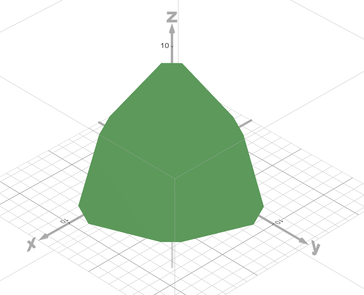
A A symmetric polytope with extreme points of $(10,2,1)$ and $(7,6,0)$ and their permutations.

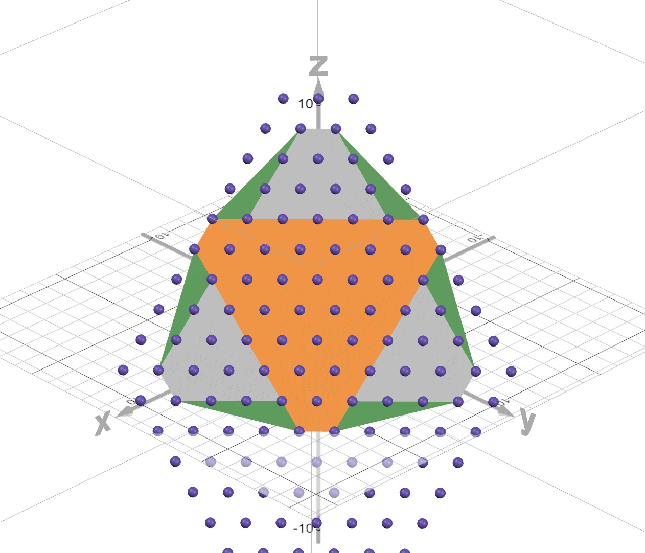
B Figure 1A with the Newton polytopes of $s_{(10,2,1)}$ and $s_{(7,6,0)}$ along with the integer points.

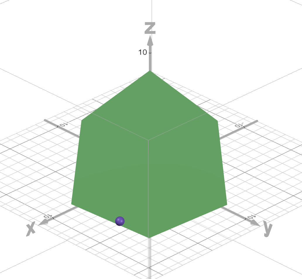
C A symmetric polytope with extreme points of $(10,2,2)$ and $(7,7,0)$ and their permutations. The point $(8,5,1)$ lies in the polytope.

Figure 1.

3. Conjecture on Symmetric Polytopes and IDP

We now discuss how one can extend ideas in [BGH⁺21, NNTDLH23] for our purposes. The authors of [BGH⁺21, NNTDLH23] used certain families of polynomials $s$ which have SNP to show that $\operatorname{Newt}(s)$, which is symmetric, has IDP. To use these same strategies, we define $s$ in the following way.

Lemma 3.1.

Let $\displaystyle s:=\sum_{\lambda\in\operatorname{MLP}(\mathcal{P})}s_{\lambda}$. Then $\mathcal{P}=\operatorname{Newt}(s)$.

The definition of convex hull and Rado’s Theorem [Rad52] provides justification for why this Lemma holds, which we detail now. Given a symmetric polytope $\mathcal{P}$ in $\mathbb{R}^{m}$, if $\lambda$ is a lattice point in $\mathcal{P}$, then so is $\pi(\lambda)$ for all permutations $\pi$ in $S_{m}$, the symmetric group on $m$ elements. Then by the definition of Newton polytopes, we see that $\operatorname{Newt}(s_{\lambda})\subseteq\mathcal{P}$. Thus, the support of $\displaystyle s=\sum_{\lambda\in\operatorname{LP}(\mathcal{P})}s_{\lambda}$ contains all lattice points of $\mathcal{P}$, so $\mathcal{P}=\operatorname{Newt}(s)$. However, by Rado’s Theorem [Rad52], we see that $\lambda\trianglelefteq\mu$ if and only if $\operatorname{Newt}(s_{\lambda})\subseteq\operatorname{Newt}(s_{\mu})$. Thus, the support of $s$ is equal to the support of $\displaystyle\sum_{\lambda\in\operatorname{MLP}(\mathcal{P})}s_{\lambda}$.

Returning now to our situation, we see that if $\lambda$ and $\mu$ are the partitions for a 2-partition maximal polytope $\mathcal{P}$ and $s:=s_{\lambda}+s_{\mu}$, then $\operatorname{Newt}(s)=\mathcal{P}$. To employ the methods of [BGH⁺21, NNTDLH23], we will want to find a polynomial with SNP which is $t\mathcal{P}$ for each choice of $t$. To this end, we define the following.

Definition 3.2.

Given $k$ partitions $\lambda_{1},\lambda_{2},\dots,\lambda_{k}$, not necessarily distinct, let $s:=s_{\lambda_{1}}+s_{\lambda_{2}}+\cdots+s_{\lambda_{k}}$. We define a new function $ts$, for $t\in\mathbb{Z}_{>0}$. Let $K:=\{1,2,\dots,k\}$ and $\left(\kern-3.00003pt\left(\genfrac{}{}{0.0pt}{}{K}{t}\right)\kern-3.00003pt\right)$ be the set of multisubsets of $K$ of size $t$. For $I\in\left(\kern-3.00003pt\left(\genfrac{}{}{0.0pt}{}{K}{t}\right)\kern-3.00003pt\right)$, let $\lambda_{I}:=\displaystyle\sum_{i\in I}\lambda_{i}$. Then

$$ts:=\displaystyle\sum_{I\in\left(\kern-2.10002pt\left(\genfrac{}{}{0.0pt}{}{K}{t}\right)\kern-2.10002pt\right)}s_{\lambda_{I}}.$$

Remark 3.3.

Note when $k=2$, $ts$ becomes

$$\sum_{i=0}^{t}s_{(t-i)\lambda_{1}+i\lambda_{2}}.$$

In general, we conjecture the following for this special choice of $ts$ whenever $\mathcal{P}$ is a symmetric polytope.

Conjecture 3.4.

For $t\in\mathbb{Z}_{>0}$, we have $\operatorname{Newt}(ts)=t\operatorname{Newt}(s)$ and thus $t\mathcal{P}=\operatorname{Newt}(ts)$. Furthermore, $ts$ has SNP for all $t$.

If this conjecture is true, then the set of lattice points of $t\mathcal{P}$ is the support of $ts$. Then we can apply the following.

Theorem 3.5.

Let $\mathcal{P}$ be a symmetric polytope for which the prior conjecture holds true for $\displaystyle s=\sum_{\lambda\in\operatorname{MLP}(\mathcal{P})}s_{\lambda}$. (That is, $s$ has SNP.) Then $\mathcal{P}$ has the integer decomposition property.

Proof.

Let $\mathcal{P}$ be a symmetric polytope for which the prior conjecture holds true. Let $t$ be a positive integer. We want to show that every lattice points of $t\mathcal{P}$ can be written as sum of $t$ lattice points of $\mathcal{P}$. Let $\pi\in t\mathcal{P}$. Since $ts$ has SNP, then $\pi$ is an exponent vector of

$$ts=\displaystyle\sum_{I\in\left(\kern-2.10002pt\left(\genfrac{}{}{0.0pt}{}{K}{t}\right)\kern-2.10002pt\right)}s_{\lambda_{I}},$$

that is, there is an $I:=\{i_{1},i_{2},\dots,i_{t}\}$ so that $\pi$ is an exponent vector of $s_{\lambda_{i_{1}}+\lambda_{i_{2}}+\cdots+\lambda_{i_{t}}}$. Each exponent vector of $s_{\lambda_{i_{1}}+\lambda_{i_{2}}+\cdots+\lambda_{i_{t}}}$ corresponds to a content vector of some semistandard tableau, which we denote $T$, for the partition $\lambda_{i_{1}}+\lambda_{i_{2}}+\cdots+\lambda_{i_{t}}$. We demonstrate that any such tableau can be decomposed into semistandard tableaux for $\lambda_{i_{1}}$, $\lambda_{i_{2}}$, $\dots$, $\lambda_{i_{t}}$, which we will denote $T_{i_{j}}$ for $j$ from $1$ to $t$ respectively. We define these using an inductive procedure, focusing on one row of each tableau at a time, starting with the last row for each.

Let $n$ be the number of rows in $T$ and let $(\lambda_{i_{j}})_{k}$ denote the $k$th part of $\lambda_{i_{j}}$. For each $j$, starting at $j=1$ do the following.

1. Let $\ell$ be the number of rows of $T$. Remove the first $(\lambda_{i_{j}})_{\ell}$ columns from $T$ and use them as the right-most columns of $T_{i_{j}}$. Note that these columns all have length $\ell$.

2. Subtract $(\lambda_{i_{j}})_{\ell}$ from each entry of $\lambda_{i_{j}}$, truncating the last coordinate.

We now can repeat these steps by inducting on the length of the partitions to find the remaining columns for $T_{i_{j}}$.

Each $T_{i_{j}}$ is a semistandard tableaux since columns of $T_{i_{j}}$ come directly from columns of $T$ and they are added from left-to-right. Each $T_{i_{j}}$ is also of shape $\lambda_{i_{j}}$. We prove this by inducting on the rows of $T_{i_{j}}$. Observe by step $1$ of the above procedure that this is true for row $n$. After the first iteration of the two steps above is completed, note that the length of the partitions decreases. In general, suppose row $r$ of $T_{i_{j}}$ has $(\lambda_{i_{j}})_{r}$ cells. Then the above procedure will add $(\lambda_{i_{j}})_{r-1}-(\lambda_{i_{j}})_{r}$ columns from $T$ to $T_{i_{j}}$, meaning that row $r-1$ will have $(\lambda_{i_{j}})_{r-1}-(\lambda_{i_{j}})_{r}+(\lambda_{i_{j}})_{r}=(\lambda_{i_{j}})_{r-1}$ cells. Furthermore, after the above steps are completed for row $r-1$, $T$ will have length $r-2$, meaning that no further cells will be added to row $r-1$.

Consequently, each $T_{i_{j}}$ has a shape that corresponds to $\lambda_{i_{j}}$, which means the content vector of $T_{i_{j}}$ is a lattice point of $\mathcal{P}$ since $s$ has SNP. Thus $\pi$, which is the content vector of $T$, can be written as a sum of $t$ lattice points of $\mathcal{P}$. This implies $\mathcal{P}$ has IDP.

∎

Example 3.6.

In Figure 2A is a semistandard tableau for the partition $(8,7,2)$, which can be decomposed into the three tableaux with shapes $\lambda=(2,2,1)$, $\mu=(4,3,1)$ and $\gamma=(2,2,0)$ using the algorithm in the prior proof.

Since the last part of $\lambda$ and $\mu$ is $1$, we start by designating the first column for $T_{\lambda}$ and the second for $T_{\mu}$ (depicted in Figure 2B).

centertableaux

1 & 1 1 2 2 3 3 3
2 2 3 3 4 4 4
3 4

A

*(red!50) 1 & *(blue!50) 1 1 2 2 3 3 3
*(red!50)2 *(blue!50) 2 3 3 4 4 4
*(red!50) 3 *(blue!50) 4

B

Figure 2. The first step of the decomposition process for a semistandard tableau of shape $(8,7,2)$.

Modifying our partitions, we now have $\lambda=(1,1,0)$, $\mu=(3,2,0)$, and $\gamma=(2,2,0)$. Continuing with the updated version of $T$, the first column is assigned to $T_{\lambda}$, the following two are assigned to $T_{\mu}$, and the following two columns are assigned to $T_{\gamma}$. At the end of this step, $T_{\lambda}$ and $T_{\gamma}$ are complete (see Figures 3B and 3D, respectively), and all but the final column of $T$ has been assigned. This final column will be assigned to $T_{\mu}$. See Figure 3A below for the identification of these columns in $T$ and the updated picture for $T_{\gamma}$ in Figure 3C.

centertableaux

*(red!50) 1 & *(blue!50) 1 *(red!50)1 *(blue!50) 2 *(blue!50) 2 *(green!50) 3 *(green!50) 3 *(blue!50) 3
*(red!50) 2 *(blue!50) 2 *(red!50)3 *(blue!50) 3 *(blue!50) 4 *(green!50) 4 *(green!50) 4
*(red!50) 3 *(blue!50) 4

A

*(red!50) 1 &*(red!50) 1
*(red!50) 2 *(red!50) 3
*(red!50) 3

B

*(blue!50) 1 &*(blue!50) 2 *(blue!50) 2*(blue!50) 3
*(blue!50) 2 *(blue!50) 3*(blue!50) 4
*(blue!50) 4

C

*(green!50) 3 &*(green!50) 3
*(green!50) 4 *(green!50) 4

D

Figure 3. Steps two and three of the decomposition process of a tableau of shape $(8,7,2)$.

As an example of an application for the prior Theorem, if $\mathcal{P}$ is a symmetric polytope with two maximal lattice partitions so that Conjecture 3.4 holds, then each lattice points of $t\mathcal{P}$ is a content vector of a semistandard Young tableau of $(t-k)\lambda+k\mu$ for $0\leq k\leq t$, which can be separated into $t-k$ content vector for $\lambda$ and $k$ for $\mu$. Note that the content vectors of $\lambda$ and $\mu$ are themselves lattice points of $\mathcal{P}$. Thus the lattice point can be written as a sum of $t$ points from $\mathcal{P}$.

Remark 3.7.

One can apply the above framework to aforementioned results. For example, consider the work done by [BGH⁺21]. There, they define the symmetric Grothendieck polynomial $G_{\lambda}$ of a partition $\lambda$ and study $\mathcal{P}=\operatorname{Newt}(G_{\lambda})$. The polynomial $G_{\lambda}$ is of the form

$$G_{\lambda}=\sum_{\mu}c_{\mu}s_{\mu}$$

where $c_{\mu}\in\mathbb{Z}$ and the sum is over partitions $\mu$ obtained by adding boxes to the Young diagram of $\lambda$. The partitions $\mu$ in the above descriptions are not all maximal partitions. However, in [EY17], they have shown that the $\mathcal{P}$ is the convex hull of the support of $\displaystyle\sum_{\mu\in\operatorname{MLP}}s_{\mu}$. In [BGH⁺21], the authors showed that $\mathcal{P}$ has IDP by observing that $t\mathcal{P}=\operatorname{Newt}(G_{t,t\lambda})$ where $t\in\mathbb{Z}_{>0}$ and $G_{t,t\lambda}$ is the inflated symmetric Grothendieck polynomial. In addition, they showed that the $t\mathcal{P}$ is the convex hull of the support of $\displaystyle\sum_{\mu\in\operatorname{MLP}(t\mathcal{P})}s_{\mu}$. Thus, one can define $s=\displaystyle\sum_{\mu}s_{\mu}$ (with maximal lattice partition $\mu$) and apply the method outlined in this section to give an alternative proof that $\mathcal{P}$ is IDP.

4. 2-Partition Maximal Polytopes and IDP

In this section we apply the method outlined in the prior section in our special case. Throughout, $\lambda$ and $\mu$ are pairwise maximal partitions corresponding to a 2-partition maximal polytope $\mathcal{P}$. We will focus on the case where the size of $\lambda$ and $\mu$ are the same, leaving the other cases for future study. Thus, $\mathcal{P}$ lies in a hyperplane. We further restrict our study to the case where $\mathcal{P}\subseteq\mathbb{R}^{3}$, meaning that the length of $\lambda$ and $\mu$ is 3, as in this case we learn even more about the partitions $\lambda$ and $\mu$.

Lemma 4.1.

If the lengths of $\lambda$ and $\mu$ are 3 and both partitions have the same size, then $|\lambda_{i}-\mu_{i}|=1$ for some $i\in\{1,2,3\}$.

Proof.

Suppose that we have $\lambda=(\lambda_{1},\lambda_{2},\lambda_{3})$ and $\mu=(\mu_{1},\mu_{2},\mu_{3})$ so that $|\lambda_{i}-\mu_{i}|\geq 2$ for all $i$. Without loss of generality, suppose $\lambda_{1}>\mu_{1}$. Thus, for $\lambda$ and $\mu$ to be maximal (and not comparable), we must have $\lambda_{3}>\mu_{3}$. Specifically, note that $\lambda_{3}>\mu_{3}+1$.

Now, let $\gamma:=(\mu_{1}+1,n-\mu_{1}-\lambda_{3},\lambda_{3}-1)$. Note that $\gamma$, $\lambda$, and $\mu$ are pairwise maximal. We prove that $\gamma\in\mathcal{P}$.

First, consider the point $\iota:=(\mu_{1},n-\mu_{1}-\lambda_{3},\lambda_{3})$. Observe that $\iota\in\mathcal{P}$ since $\mu$ and $\lambda$ dominate $\iota$. Thus, it is sufficient to show that $\gamma\in\operatorname{conv}(\lambda,\mu,\iota)$. To this end, we define a matrix $A=\begin{bmatrix}\lambda&\mu&\iota\end{bmatrix}$, that is, a $3\times 3$ matrix whose columns are $\lambda$, $\mu$, and $\iota$. We will demonstrate that $A^{-1}$ exists and $A^{-1}\gamma$ has non-negative entries which sum to $1$.

To proceed, we use Sage’s Matrix class to perform the necessary computations. These can be seen in Appendix A. First, the determinant of $A$ is

$$\big{(}\lambda_{3}(\mu_{1}+\mu_{2})-\mu_{3}(\lambda_{1}+\lambda_{2})\big{)}(\lambda_{1}-\mu_{1})=n(\lambda_{3}-\mu_{3})(\lambda_{1}-\mu_{1})$$

which is nonzero since $\lambda_{1}>\mu_{1}$ and $\lambda_{3}>\mu_{3}$, and so $A^{-1}$ exists.

We next demonstrate that the entries of $A^{-1}\gamma$ sum to $1$. After computation, we find that

$$A^{-1}\gamma=\begin{bmatrix}{1\over(\lambda_{1}-\mu_{1})}&{1\over(\lambda_{3}-\mu_{3})}&1+{\lambda_{2}-\mu_{2}\over(\lambda_{1}-\mu_{1})(\lambda_{3}-\mu_{3})}\end{bmatrix}.$$

If one adds the first two entries together, utilizing the fact that the size of $\lambda$ and $\mu$ are the same, we have

$${1\over(\lambda_{1}-\mu_{1})}+{1\over(\lambda_{3}-\mu_{3})}={\lambda_{1}+\lambda_{3}-(\mu_{1}+\mu_{3})\over(\lambda_{1}-\mu_{1})(\lambda_{3}-\mu_{3})}={\mu_{2}-\lambda_{2}\over(\lambda_{1}-\mu_{1})(\lambda_{3}-\mu_{3})},$$

which when added the final entry of $A^{-1}\gamma$ gives $1$. Now, since $\lambda_{1}>\mu_{1}$ and $\lambda_{3}>\mu_{3}$, one can see the first two entries of $\gamma$ are positive. Since the last entry is $1$ minus the first two entries of $\gamma$, both of which are at most ${1\over 2}$ due to our assumption that $|\lambda_{i}-\mu_{i}|\geq 2$, this means the final entry is non-negative. That is, we have demonstrated that $\gamma\in\operatorname{conv}(\lambda,\mu,\iota)\subseteq\mathcal{P}$. This means that $\{\lambda,\mu,\gamma\}\subseteq\operatorname{MLP}(\mathcal{P})$, but we assumed that $\mathcal{P}$ is $2$-partition-maximal. This is a contradiction.

Thus, we know there exists an $i$ for which $|\lambda_{i}-\mu_{i}|\leq 1$. However, we now further that this value can not be $0$. However, since the length of $\mu$ and $\lambda$ are 3, if one of their coordinates agree, then after removing these coordinates we are really considering partitions of length 2 with the same size. These partitions are always comparable, contradicting that our partitions are pair-wise not comparable.

∎

In the prior proof, we utilized the region $\operatorname{conv}(\lambda,\mu,\iota)$ with $\iota:=(\mu_{1},n-\mu_{1}-\lambda_{3},\lambda_{3})$. This region has further utility.

Lemma 4.2.

The interior of $\operatorname{conv}(\lambda,\mu,\iota)$ contains all weakly decreasing lattice points in $\mathcal{P}$ which are not contained in $\operatorname{Newt}(s_{\lambda})$ and $\operatorname{Newt}(s_{\mu})$.

Proof.

For convenience we define $N_{\lambda}:=\operatorname{Newt}(s_{\lambda})$ and $N_{\mu}:=\operatorname{Newt}(s_{\mu})$.

First, we demonstrate $\operatorname{Ext}(\mathcal{P})=\operatorname{Ext}(N_{\lambda})\cup\operatorname{Ext}(N_{\mu})$. By Lemma 3.1, $\mathcal{P}$ is the convex hull of the exponent vectors for $s_{\lambda}$ and $s_{\mu}$. Without loss of generality, suppose $\pi\in\operatorname{Ext}(\mathcal{P})$ is an exponent vector of $s_{\lambda}$. If $\pi$ were not an extreme point of $N_{\lambda}$, then it is either on the boundary or interior of $N_{\lambda}$. Then the same would be true for $\mathcal{P}$, which is a contradiction. On the other hand, suppose $\pi\in\operatorname{Ext}(N_{\lambda})\cup\operatorname{Ext}(N_{\mu})$ and yet $\pi\notin\operatorname{Ext}(N_{s})$. Without loss of generality, $\pi\in\operatorname{Ext}(N_{\mu})$, which implies that $\pi$ is one of the permutations of $\mu$. By definition of $N_{s}$, if $\pi\not\in\operatorname{Ext}(N_{s})$, then none of the other permutations of $\pi$ is an extreme point of $N_{s}$.Then $\operatorname{Ext}(N_{s})\subseteq\operatorname{Ext}(N_{\lambda})$. This implies that $N_{s}\subseteq N_{\lambda}$. Thus $\mu\in N_{s}$ is a lattice point in $N_{\lambda}$, which means that $\mu$ is dominated by $\lambda$. However, this contradicts that $\mu$ and $\lambda$ are not comparable.

Next, we demonstrate that $\iota=(\mu_{1},n-\mu_{1}-\lambda_{3},\lambda_{3})$ is both on a facet of $N_{\lambda}$ and $N_{\mu}$. Using [BGH⁺21, Theorem 29], note that $\iota$ is on the face defined by $x+y=\lambda_{1}+\lambda_{2}$, and so $\iota$ is on a facet of $N_{\lambda}$, and $\iota$ is on the face defined by $x=\mu_{1}$, so $\iota$ is also on a facet of $N_{\mu}$.

The line $(\lambda_{3}-\mu_{3})x-(\lambda_{1}-\mu_{1})z=\mu_{1}\lambda_{3}-\mu_{3}\lambda_{1}$ has both $\lambda$ and $\mu$ on it. We claim this line is a facet of $\mathcal{P}$, that is, $(x,y,z)\in\mathcal{P}$ implies $(\lambda_{3}-\mu_{3})x-(\lambda_{1}-\mu_{1})z\leq\mu_{1}\lambda_{3}-\mu_{3}\lambda_{1}$. Note that for all permutations $(x,y,z)$ of $\lambda$, $x\leq\lambda_{1}$ and $z\geq\lambda_{3}$. Thus

$$(\lambda_{3}-\mu_{3})x-(\lambda_{1}-\mu_{1})z\leq (\lambda_{3}-\mu_{3})\lambda_{1}-(\lambda_{1}-\mu_{1})\lambda_{3}$$

$$= \lambda_{3}\mu_{1}-\lambda_{1}\mu_{3}.$$

Note that for all permutations $(x,y,z)$ of $\mu$, $x\leq\mu_{1}$ and $z\geq\mu_{3}$. Thus

$$(\lambda_{3}-\mu_{3})x-(\lambda_{1}-\mu_{1})z\leq (\lambda_{3}-\mu_{3})\mu_{1}-(\lambda_{1}-\mu_{1})\mu_{3}$$

$$= \lambda_{3}\mu_{1}-\lambda_{1}\mu_{3}.$$

We have demonstrated that the extreme points of $\mathcal{P}$ satisfy the aforementioned inequality, and thus every point in $\mathcal{P}$ does as well.

We now can finally demonstrate that the decreasing points of $\mathcal{P}$ are contained in $\operatorname{conv}(\lambda,\mu,\iota)$. We first identify the facet defining inequalities of $\operatorname{conv}(\lambda,\mu,\iota)$. There are three facets: hyperplanes containing $\mu$ and $\lambda$, $\iota$ and $\mu$, and $\iota$ and $\lambda$. That is, the points of $\operatorname{conv}(\lambda,\mu,\iota)$ satisfy the following three inequalities:

$$(\lambda_{3}-\mu_{3})x-(\lambda_{1}-\mu_{1})z\leq\mu_{1}\lambda_{3}-\mu_{3}\lambda_{1},\,\,\,x\geq\mu_{1},\,\,\,\text{and }z\leq\lambda_{3}.$$

Let $(x,y,z)\in\mathcal{P}\setminus(N_{\lambda}\cup N_{\mu})$ and $x\geq y\geq z$. Since $(x,y,z)\not\in N_{\lambda},$ it must not satisfy at least one of the facet defining inequalities from [BGH⁺21, Theorem 29]:

$$x\leq\lambda_{1}, \hskip 8.5359ptx\geq\lambda_{3},$$

$$y\leq\lambda_{1}, \hskip 8.5359pty\geq\lambda_{3},$$

$$z\leq\lambda_{1}, \hskip 8.5359ptz\geq\lambda_{3}.$$

Since $x\geq y\geq z$, one of $x\leq\lambda_{1}$ or $z\geq\lambda_{3}$ must not be satisfied. However, $(x,y,z)\in\mathcal{P}$, which is the convexhull of permutations of $\lambda$ and $\mu$. Since the coordinates of $\lambda$ and $\mu$ are at most $\lambda_{1}$, $x$, $y$, and $z$ cannot be more than $\lambda_{1}$. Thus $x\leq\lambda_{1}$ is always satisfied. Further, $z<\lambda_{3}$.

Similarly, since $(x,y,z)\not\in N_{\mu},$ $x\leq\mu_{1}$ or $z\geq\mu_{3}$ must not be satisfied. But as before, since the coordinates of $\lambda$ and $\mu$ are at least $\mu_{3},$ we know that $z\geq\mu_{3}$. Thus $x>\mu_{1}$. Thus, we have demonstrated that any decreasing point in $\mathcal{P}$ satisfies the three aforementioned facet defining inequalities. ∎

The utility of this result is two-fold. First, recall that ultimately our goal is to show that if $s=s_{\lambda}+s_{\mu}$, we have $ts$ is SNP for all $t\in\mathbb{N}$. Since it is already known that $s_{\lambda}$ and $s_{\mu}$ are SNP, we need only be concerned with points outside the Newton polytope for these two points. Beyond this, we also know that a point $\pi\in\mathcal{P}$ if and only if a permutation of $\pi$ is in $\mathcal{P}$. Thus, we may only concern ourselves with decreasing points outside of the Newton polytopes of $s_{\lambda}$ and $s_{\mu}$, that is, the interior of the region $\operatorname{conv}(\lambda,\mu,\iota)$. With the prior Lemma in mind, we have the following from which Theorem 1.1 follows.

Theorem 4.3.

The polynomial

$$ts=\sum_{i=0}^{t}s_{(t-i)\lambda+i\mu}$$

has SNP.

Proof.

We show $(x,y,z)\in\operatorname{Newt}(s_{(t-i)\lambda+i\mu})$ for some $i$. By Lemma 4.1, we know there exists a coordinate between $\lambda$ and $\mu$ which differs exactly by $1$. Without loss of generality, suppose $\lambda_{3}-\mu_{3}=1$. Then $t\mu_{3}\leq z\leq t\lambda_{3}$. Let $\alpha:=(t-(t\lambda_{3}-z))\lambda+(t\lambda_{3}-z)\mu$. We claim that $(x,y,z)\in\operatorname{Newt}(s_{\alpha})$.

Observe the last coordinate of $\alpha$ is $z$, since

$$(t-(t\lambda_{3}-z))\lambda_{3}+(t\lambda_{3}-z)\mu_{3}= t\lambda_{3}-t\lambda_{3}\lambda_{3}+z\lambda_{3}+t\lambda_{3}\mu_{3}-z\mu_{3}$$

$$= t\lambda_{3}+z(\lambda_{3}-\mu_{3})-t\lambda_{3}(\lambda_{3}-\mu_{3})$$

$$= z,$$

where the last equality follows after implementing our assumption that $\lambda_{3}-\mu_{3}=1$.

By assuming $(x,y,z)$ is weakly decreasing, recall by Lemma 4.2 we know that $(x,y,z)\in\operatorname{conv}(\lambda,\mu,\iota)$ where $\iota:=(\mu_{1},n-\mu_{1}-\lambda_{3},\lambda_{3})$. Thus, we may write $(x,y,z)=at\lambda+bt\mu+ct\iota$ with $a,b,c>0$ and $a+b+c=1$. Since the last coordinates of $(x,y,z)$ and $\alpha$ are equal, we just need to show that $x$ is less than the first coordinate of $\alpha$, that is,

$$at\lambda_{1}+bt\mu_{1}+ct\mu_{1}<(t-(t\lambda_{3}-z))\lambda_{1}+(t\lambda_{3}-z)\mu_{1}=t\lambda_{1}-(t\lambda_{3}-z)(\lambda_{1}-\mu_{1}).$$

Since $z=at\lambda_{3}+bt\mu_{3}+ct\lambda_{3}$, we have

$$t\lambda_{3}-z=t\lambda_{3}-(at\lambda_{3}+bt\mu_{3}+ct\lambda_{3})=t((1-a-c)\lambda_{3}-b\mu_{3})=t(b\lambda_{3}-b\mu_{3})=tb(\lambda_{3}-\mu_{3})=tb.$$

Thus,

$$t\lambda_{1}-(t\lambda_{3}-z)(\lambda_{1}-\mu_{1})= t\lambda_{1}-tb(\lambda_{1}-\mu_{1})$$

$$= t(\lambda_{1}-b\lambda_{1}+b\mu_{1})$$

$$= t((1-b)\lambda_{1}+b\mu_{1}).$$

Note that since $\mu_{1}<\lambda_{1}$, we have

$$x=at\lambda_{1}+bt\mu_{1}+ct\mu_{1}< at\lambda_{1}+bt\mu_{1}+ct\lambda_{1}$$

$$= t(b\mu_{1}+(a+c)\lambda_{1})$$

$$= t(b\mu_{1}+(1-b)\lambda_{1})=t\lambda_{1}-(t\lambda_{3}-z)(\lambda_{1}-\mu_{1}).$$

That is, we have now shown that $(x,y,z)$ is dominated by $\alpha$. ∎

Corollary 4.4 (Theorem 1.1).

$\mathcal{P}$ has IDP.

Proof.

This follows from Theorem 4.3 and Theorem 3.5. ∎

Appendix A Sage

The following was used to aid in computations. To be used for Lemma 4.1, we let $\lambda_{1}=a$, $\lambda_{2}=b$, $\lambda_{3}=c$, $\mu_{1}=d$, $\mu_{2}=e$, and $\mu_{3}=f$. Thus, the matrix $A$ is $[\lambda\ \mu\ \iota]$. Note in place of $n-\mu_{1}-\lambda_{3}$ we use $\lambda_{1}+\lambda_{2}-\mu_{1}$, keeping in mind that $n=\lambda_{1}+\lambda_{2}+\lambda_{3}$, and this identity was used extensively in translating and simplifying the following output.

var(”a”,”b”,”c”,”d”,”e”,”f”) A=Matrix([[a,d,d],[b,e,a+b-d],[c,f,c]]) print(A.determinant().expand())

a*c*d - c*d^2 + a*c*e - c*d*e - a^2*f - a*b*f + a*d*f + b*d*f

B=A.inverse() gamma=vector([d+1,a+b-d,c-1]) X=vector(B*gamma) print(X.simplify_full())

(-((a + b)*d - d^2 - (c + d)*e + (a + b - d)*f)/
(a*c*d - c*d^2 + (a*c - c*d)*e - (a^2 + a*b - (a + b)*d)*f),
(a + b + c)/(c*d + c*e - (a + b)*f),
-(c*d^2 - (a*c + b)*d - ((a - 1)*c - c*d - a)*e + (a^2 + (a - 1)*b - (a + b)*d)*f)/
(a*c*d - c*d^2 + (a*c - c*d)*e - (a^2 + a*b - (a + b)*d)*f))

References

- [BGH+21] Margaret Bayer, Bennet Goeckner, Su Ji Hong, Tyrrell McAllister, McCabe Olsen, Casey Pinckney, Julianne Vega, and Martha Yip. Lattice polytopes from schur and symmetric grothendieck polynomials. Electronic Journal of Combinatorics, 28, 2021. doi:10.37236/9621.
- [CLS24] David A Cox, John B Little, and Henry K Schenck. Toric varieties, volume 124. American Mathematical Society, 2024.
- [EY17] Laura Escobar and Alexander Yong. Newton polytopes and symmetric Grothendieck polynomials. C. R. Math. Acad. Sci. Paris, 355(8):831–834, 2017. doi:10.1016/j.crma.2017.07.003.
- [Ful93] William Fulton. Introduction to toric varieties. Number 131. Princeton university press, 1993.
- [KKE21] B Ya Kazarnovskii, Askold Georgievich Khovanskii, and Alexander Isaakovich Esterov. Newton polytopes and tropical geometry. Russian Mathematical Surveys, 76(1):91, 2021.
- [MTY19] Cara Monical, Neriman Tokcan, and Alexander Yong. Newton polytopes in algebraic combinatorics. Selecta Mathematica, 25(5):66, 2019.
- [NNTDLH23] Duc-Khanh Nguyen, Giao Nguyen Thi Ngoc, Hiep Dang Tuan, and Thuy Do Le Hai. Newton polytope of good symmetric polynomials. Comptes Rendus. Mathématique, 361(G4):767–775, 2023.
- [Rad52] R. Rado. An inequality. J. London Math. Soc., 27:1–6, 1952. doi:10.1112/jlms/s1-27.1.1.
- [TOG17] Csaba D Toth, Joseph O’Rourke, and Jacob E Goodman. Handbook of discrete and computational geometry. CRC press, 2017.