[main-]../auxiliary
A cautious use of auxiliary outcomes for decision-making in randomized clinical trials.
Abstract
Clinical trials often collect data on multiple outcomes, such as overall survival (OS), progression-free survival (PFS), and response to treatment (RT). In most cases, however, study designs only use primary outcome data for interim and final decision-making. In several disease settings, clinically relevant outcomes, for example OS, become available years after patient enrollment. Moreover, the effects of experimental treatments on OS might be less pronounced compared to auxiliary outcomes such as RT. We develop a Bayesian decision-theoretic framework that uses both primary and auxiliary outcomes for interim and final decision-making. The framework allows investigators to control standard frequentist operating characteristics, such as the type I error rate, and can be used with auxiliary outcomes from emerging technologies, such as circulating tumor assays. False positive rates and other frequentist operating characteristics are rigorously controlled without any assumption about the concordance between primary and auxiliary outcomes. We discuss algorithms to implement this decision-theoretic approach and show that incorporating auxiliary information into interim and final decision-making can lead to relevant efficiency gains according to established and interpretable metrics.
Keywords: Auxiliary variables, breast cancer, decision theory, glioblastoma, multiple hypothesis testing, trial design
1 Introduction
Clinical trials evaluate the efficacy and safety of experimental treatments. In most cases, regulatory decisions about the efficacy of treatments are based on the comparison of primary outcomes under the experimental treatment and the standard of care (SOC). In oncology, these comparisons typically attempt to demonstrate improvements of the overall survival (OS). However, in several disease settings, collecting data on OS requires long follow-up times. Therefore, using only OS for decision-making may be inefficient and expose patients to potentially ineffective experimental treatments.
Auxiliary and surrogate outcomes are available earlier than primary outcomes. In some cases, they provide stronger signals of positive effects than the primary outcomes (Pilz et al.,, 2012), and reduce the size and duration of the trial (e.g., Ellenberg and Hamilton,, 1989; Chen et al.,, 2019). In oncology, several surrogates of OS have been used for regulatory decision-making, including progression-free survival (PFS), response to treatment (RT), and reduction of tumor size (Kemp and Prasad,, 2017).
An ideal surrogate outcome fully captures, without ambiguity or risks, the effects of the experimental treatment on the primary outcome. We refer to Prentice, (1989) and Buyse and Molenberghs, (1998) for formal definitions of the concept of surrogate outcome. In many disease settings, the ideal relationship between treatment effects on primary and surrogate outcomes remains hypothetical, controversial, or difficult to demonstrate. In fact, clinical research provides many examples of analyses based on primary and surrogate outcomes that led to opposing conclusions on the efficacy of experimental therapies. For example, in glioblastoma, lomustine in combination with bevacizumab has been reported to improve PFS compared to lomustine alone, but later trials suggested a lack of effects on OS (Wick et al.,, 2017).
There is extensive literature on criteria and methods to evaluate the agreement between the assessment of experimental therapies based on the primary outcomes and the one based on surrogate (e.g., Buyse et al.,, 2000; Elliott et al.,, 2014; Vandenberghe et al.,, 2018). If evidence from previous trials, meta-analyses, and validation studies suggests strong agreement, investigators might consider using the surrogate outcome as primary endpoint in future trials, discussing and accounting for potential advantages and risks.
In this paper, we discuss the use of auxiliary outcomes (e.g., tumor response in glioblastoma), which have not been validated through comprehensive analyses with stringent criteria, the necessary prerequisite to replace the primary outcomes in a clinical trial. We investigate if and how auxiliary outcomes are relevant in clinical studies to support decision-making.
We develop a method to make interim and final decisions—such as recommendations for treating future patients with the experimental therapy—in clinical trials by considering primary and auxiliary outcomes and accounting for strict regulatory requirements on the accuracy of the study’s final results. Notable examples of regulatory requirements include the control of the probability of a false positive result and the control of the family-wise error rate (FWER) if the treatment is tested in multiple subgroups. We illustrate the potential advantages of joint modeling of auxiliary and primary outcomes, in two common examples:
1-Trials designs with patient subgroups. The aim is to provide subgroup-specific evidence of positive treatment effects while controlling the FWER (e.g., LeBlanc et al.,, 2009; Chugh et al.,, 2009). In this case, auxiliary outcomes can help identify the subgroups that benefit most from the experimental treatment, improving the likelihood of reporting positive results without compromising the control of the FWER.
2-Multi-stage trial designs (e.g., Simon,, 1989; Ensign et al.,, 1994). Here, auxiliary outcomes can support early futility decisions while ensuring power above a desired threshold and strict control of the probability of a false positive result.
In both cases, the regulatory constraints are standard frequentist requirements.
In our method, primary and auxiliary outcomes are incorporated into decision-making using a Bayesian decision-theoretic framework (Berger,, 1985). Throughout the paper, the optimal clinical trial design, which includes a detailed plan for interim and final decisions, coincides with the solution of a constrained maximization problem defined by three key components: (i) a utility function (Lindley,, 1976); (ii) a Bayesian prior model representative of previous studies that includes primary and auxiliary outcomes; and (iii) constraints on frequentist operating characteristics, such as the rigorous control of the probability of a false positive result below a pre-specified level, enforced across all potential scenarios in which the experimental treatment does not improve the primary outcomes. The design is optimized using a Bayesian model and satisfies frequentist characteristics. Our approach can be applied to select the sample size, develop a detailed plan of interim and final analyses, and choose other aspects of the study design.
The optimal design maximizes the expected utility within a subset of candidate study designs that satisfy interpretable constraints on major frequentist operating characteristics (e.g., FWER or power). Our approach builds on an informative prior distribution that reflects relevant relationships between the primary and auxiliary outcomes identified in previous studies. The prior model can incorporate variations of treatment effects across patient subgroups defined by relevant biomarkers (see Section 5).
Indeed, there is a rich literature, including meta-analyses and disease-specific summaries on the agreement between treatment effects on primary and auxiliary outcomes across trials (e.g., Mushti et al.,, 2018; Xie et al.,, 2019; Belin et al.,, 2020). We note that the correlation between auxiliary and primary outcomes does not imply proportionality between the effects on auxiliary and primary outcomes, and it is not an adequate criterion to assess a candidate surrogate outcome (Ciani et al.,, 2023). For example, in glioblastoma, several promising phase II trials that investigated effects on tumor response have been followed by phase III trials that did not demonstrate the beneficial effects of the experimental therapies on survival. Accordingly, prior models can include correlated auxiliary and primary outcomes and allow for discordant effects of experimental therapies on auxiliary and primary outcomes. The prior model can also incorporate variations of treatment effects across patient subgroups defined by relevant biomarkers. Importantly, our procedures in Sections 5 and 6 control the false positive results in the absence of positive effects on the primary outcome.
Bayesian decision theory has been used to design clinical trials (Lewis and Berry,, 1994; Ventz and Trippa,, 2015; Thall,, 2019). This framework is useful for selecting a study design or a method, such as a testing procedure, among candidate designs/methods through an interpretable measure of utility (or loss) of the trial, tailored to the study aims (Arfè et al.,, 2020). To the best of our knowledge, previous contributions did not investigate Bayesian designs that include auxiliary outcomes and attain a frequentist control of false positive results in any scenario without positive effects on the primary outcomes. We show that using auxiliary outcomes for interim and final decisions can increase the utility of the clinical trial without compromising the rigorous control of frequentist operating characteristics, such as the FWER.
The control of frequentist characteristics is an important aspect of our approach compared to other Bayesian designs. In particular, with most Bayesian designs, simulations are necessary to evaluate how key operating characteristics, including false positive rates, vary across scenarios. Selection of an appropriate set of representative scenarios can be problematic (Larry Han and Trippa,, 2024) because a few scenarios without treatment effects might be insufficient to assess how the false positive rate varies across potential joint distributions of covariates and outcomes. Throughout the paper, we compared alternative designs with the same regulatory constraints to illustrate power and simplify the interpretation of the simulation results. For these comparisons, we used simulations under realistic scenarios. In particular, we considered scenarios with positive treatment effects on primary outcomes and potential concordance/discordance with the effects on the auxiliary outcomes, which are necessary to assess the likelihood of the proposed trial designs to demonstrate the efficacy of novel therapeutics.
The paper proceeds as follows: Sections 2 and 3 introduce the notation and explain how we leverage auxiliary outcomes in major decisions during and at the end of clinical trials. Section 4 describes an approximation strategy that can be used to implement our method. Sections 5 and 6 discuss the operating characteristics of designs obtained with our method based on simulations and compare them with alternative procedures. Finally, Section 7 provides a brief discussion.
We provide practical computational procedures to approximately identify the optimal trial designs that satisfy a set of frequentist operating characteristics chosen by the user. The code is available at https://github.com/rMassimiliano/primary_and_auxiliary.
2 Primary and auxiliary outcomes
2.1 Notation
We consider a clinical trial that enrolls up to patients and compares an experimental treatment to the SOC in pre-defined patient subgroups. The subgroups can be defined through demographics and/or biomarker measurements, and indicates the number of enrollments to subgroup by the end of the trial. Here, is random because the trial enrolls from an eligible patient population without pre-enrollment information about the individual subgroups.
Data and prior model. For each patient in subgroup , we use to indicate the primary outcome (e.g., OS), is an auxiliary outcome (e.g., RT), and indicates the assignment to the SOC () or experimental treatment (). Throughout the paper we assume that patients are randomized to the SOC or experimental treatment. In the following indicate the data () and the distributions () for subgroups , with unknown parameters . We use for the joint distribution of the data , including patients from various subgroups, and to refer to the sample space. We use , to indicate the primary outcome data. Information on the unknown parameters is expressed through a prior distribution on .
Treatment effects on the primary outcomes. Treatment effects on the primary outcome in group can be quantified by a summary , where indicates a positive treatment effect in group . For example, indicates the subgroup-specific difference of the average primary outcome under the experimental treatment and the SOC. We test subgroup-specific null hypotheses for groups .
Sequential decisions. In clinical trials, data are often analyzed sequentially at interim analyses (IAs) in stages, potentially leading to major decisions such as early termination of the study or an increase of the sample size . When necessary (see Section 6), we use the superscript to indicate data up to stage , and to indicate data up to the -th stage of the trial, for , with
2.2 Optimization problem
Actions. During the trial, binary decisions (or actions) are made. For example, when and , the decisions , might refer to continuing () or stopping () the study early for futility at IA , and reporting evidence of treatment effects () or not () at the end of the trial.
Decision functions. Decisions during the trial are made using a function which maps available data into actions . For example, futility IAs and the final analysis (FA) at times use the accumulated data up to stage . In this case, the decision function is . We let indicate the space of all potential decision functions that can be used during the trial.
Regulatory constraints. The decision function has to meet regulatory requirements that have a frequentist interpretation, such as controlling the FWER. Constraints are formalized by the inequality , where the expectation is with respect to the unknown distribution of the data and is design and regulator specific. For example, when and is the result of the final analysis testing treatment effects, the function indicates if there is a false positive result or not. Therefore, if for every , then controls the type I error rate at level . Similarly, when testing for subgroups, with and , the function can be used to control the FWER. The expectation is equal to the probability of reporting at least one false positive result . For a specific function , we let indicate the set of decision functions that satisfy the regulatory constraints for all . We use to indicate the subset of decision functions that satisfy the regulatory constraints and ignore the auxiliary outcome, i.e., those that use only the available information on the primary outcomes .
Utility functions. In what follows indicates a utility function, which depends on the unknown parameters and the actions . Choosing an appropriate utility function is crucial in our framework and when implementing a decision-theoretic procedure in general. In clinical trials, the utility function typically summarizes the study’s costs and the potential benefits of demonstrating the efficacy of an experimental therapy, representing relative preferences and making explicit the goals of the study. We refer to Thall, (2019) and Lee et al., (2022) for examples and discussions on the elicitation of utility functions in cancer research. These authors, among others, developed utility functions that capture multiple aspects of a clinical study, such as drug-related adverse events and patient quality of life.
When , , and the action coincides with rejecting or not the null hypotheses , then an interpretable utility function includes a unitary reward for each true positive result and a penalty for each false positive result. In some studies, this utility function can represent economic interests and explicitly compares potential gains and costs associated with true and false positive subgroup-specific results. Importantly, other utility functions can represent different interests, for example, the life expectation of future patients diagnosed with a specific disease during a horizon of 10 years; see Berry and Eick, (1995) for an example.
Translating primary and auxiliary outcomes into actions. In the Bayesian decision-theoretic framework (Berger,, 1985), without regulatory restrictions, the decision maker selects the decision function that maximizes the expected utility , where the expectation is computed with respect to the joint distribution of the data and the parameters . Note that translates both the available primary and auxiliary data into actions
The decision-theoretic paradigm with regulatory constraints. In clinical trials, investigators are typically required to use study designs with decision functions that satisfy appropriate regulatory constraints: for all . In this setting, the investigator can select the decision function that maximizes the expected utility among those that are compliant with the regulatory constraints,
| (1) |
For example, the constraint can be used to consider only testing procedures that control the type I error rate at a desired -level in all scenarios without positive effects on the primary outcomes.
The maximization in expression (1) in most cases is analytically intractable. In Section 4 we will consider approximations of this optimization problem.
| primary outcome, subject in group | |
| auxiliary outcome, subject in group | |
| treatment assignment, subject in group | |
| trial data | |
| trial data excluding auxiliary outcomes | |
| distribution of the clinical trial dataset | |
| group-specific parameters | |
| prior distribution | |
| prior model | |
| treatment effects on the primary outcome in group | |
| a vector of actions | |
| decision function that maps data into actions | |
| space of decision functions | |
| space of regulator-compliant decision functions; | |
| space of regulator-compliant decision functions that do not use information on the auxiliary outcomes | |
| optimal choice within , ignoring the regulatory constraints | |
| optimal choice within , compliant with the regulatory constraints | |
| optimal choice within , compliant with the regulatory constraints | |
| utility expressed as a function of actions and unknown parameters |
3 Auxiliary outcomes can improve decisions
We use a stylized example to illustrate that auxiliary outcomes can improve the expected utility of the trial design. In this example, we compare the utility of an optimal decision function with complete (auxiliary and primary) information and an optimal decision function without access to auxiliary information. We focus on a simple study design that enrolls patients from a single population—without subgroups—and a single decision (hypothesis testing) at the end of the trial, . Here we omit the indices and and use and instead of and .
In this stylized example, and are two sets of testing procedures that control the type I error rate at level , i.e., . In other words, if the null hypothesis holds, then for every . Recall that functions in leverage primary and auxiliary outcome data, while functions in only use the primary outcome data. Although most of this paper focuses on randomized clinical trials, to simplify the presentation in Example 3.1 we consider a stylized setting with a single arm, a sample size equal to one, and known probability of a positive primary outcome under the control therapy.
Example 3.1 We consider a single-arm trial with binary primary and auxiliary outcomes . The outcomes and are independent, with and . The probability of a positive primary outcome under the control therapy is known and equal to The study tests the null hypotheses versus , and the utility function is
| (2) |
The utility function assigns a reward of unit to the action (reject ) when , a loss of units if and , while it is equal to zero otherwise.
We assume that prior studies suggest concordance between auxiliary and primary outcomes. This is expressed through the prior distribution , with combined with a deterministic relation between and . In particular, for every value of , and symmetrically for every . Here is a probability distribution that assigns probability to a single point and everywhere else.
For simplicity, and the sets of candidate decision functions with full information and with partial information include only non-randomized decisions (i.e., the decision functions that map the data into ).
In this example, we can enumerate the functions in . Since there are only four possible configurations of the study dataset , , , or , the full set of candidate decision functions has cardinality . Only functions in satisfy the regulatory constraint. In particular, there are two functions in that control the type I error rate and do not use auxiliary information:
(i) never rejects , i.e. , with expected utility 0, and
(ii) rejects when , i.e. , with expected utility .
There are two other candidate decision functions in that control the type I error rate and leverage auxiliary information:
(iii) rejects when , i.e. , with expected utility , and
(iv) rejects when , i.e. , with expected utility .
Although counterintuitive, the decision function (iv) is a legitimate -level test. Note that the optimal decision function with full information has higher expected utility () than the optimal decision function with partial information ().
This is a stylized example with an informative and restrictive prior on that can be easily modified to obtain a slightly different prior with full support (i.e., ). The example shows that auxiliary information can improve the expected utility compared to decision functions without auxiliary information.
However, the use of auxiliary outcomes does not always improve the expected utility of the clinical trial when we compare the optimal decision functions and . For example, consider the utility function (2) without the cost associated with false positive results () when holds but . After changing the utility function, the solution of the constrained optimization (1), coincides with the -level test that maximizes the Bayesian expected power (BEP), that is
| (3) |
The solution of (3) could be a randomized test. In this case, the decision function maps the data into the interval (Lehmann and Romano,, 2006). Randomized tests are rarely used in practice, but they can be helpful to understand some relationships between and . In Proposition 1 below, we consider randomized tests, and again . The proposition considers two sets of random variables ( and ). The whole class of possible distributions is indexed by , and the null hypothesis is an arbitrary subclass of distributions, i.e. a subset of . For simplicity we consider a single-arm study. The proposition states that there exists at least one -level test that maximizes the BEP, expression (3), without leveraging auxiliary information (i.e., ).
Proposition 1.
The set contains at least one decision function in
Proof.
Let be a solution of (3). This function maps the data into the interval . We define , where is the conditional distribution of given . The function maps the primary information into the interval and does not depend on . Moreover,
It remains to show that controls the type I error rate at level . For a general
where is the distribution of when . The last inequality follows from the fact that the product identifies a joint distribution for in and . Note that and were defined without assuming the independence of primary and auxiliary outcomes across patients. ∎
Proposition 1 is aligned with the results of Kopp-Schneider et al., (2019), who consider auxiliary information external to the trial (e.g., real-world data) instead of auxiliary information from the clinical trial, as in our approach. The authors demonstrate that if a uniformly most powerful test exists, then the power cannot be improved by leveraging external information.
In our settings, Proposition 1 shows that the auxiliary data cannot improve the expected utility for a specific combination of prior model , regulatory constraints , and utility function . This, however, does not happen in other settings. In Sections 5 and 6, we will provide realistic examples where including auxiliary data increases the expected utility and results in substantial improvements of relevant operating characteristics.
4 Approximation of the optimal solution
For most clinical studies, solving the constraint maximization problem (1) is challenging or unfeasible. It requires considering the space of functions and evaluating whether candidate functions satisfy the inequality to determine if they are in or not. Here we propose approximations and restrict the maximization problem (1) to a convenient subset of functions .
Data summaries . It is practical and intuitive to specify the subset by including decision functions that map a vector of data summaries , such as estimates of the treatment effects on primary and auxiliary outcomes, into decisions, . If is a sufficient statistic for , then there is no loss of information; standard decision-theoretic results indicate that an optimal decision is a function of sufficient statistics. More generally, informative data summaries can be the basis for nearly optimal decisions in with minimal reductions of the expected utility. Moreover, the use of low-dimensional summaries simplifies the task of interpreting candidate decision functions. For example, if includes treatment effect estimates, say the difference of the mean primary and auxiliary outcomes in the experimental and SOC arms, then each function in directly translates the estimates of the experimental treatment efficacy into decisions. In the next sections, we further discuss the interpretability of decision functions through examples.
Polynomial functions and other parametric approximations (). We further simplify the problem and restrict our selection of decision functions to parametric maps mediated by . The candidate decision functions become . These functions of are parameterized by vectors . The subset is specified to achieve a sufficient degree of flexibility through (i) an appropriate choice of the family of approximating functions and (ii) the number of parameters . For example, for a single decision , and a single data summary, we can use the sign of a -degree polynomial to make a decision, say testing a generic hypothesis. In this example, polynomials can approximate any arbitrarily well on an interval by increasing .
Regulatory constraints on parametric decision functions. Once and have been specified, we define as the subset of parametric functions that satisfy the regulatory constraints. Next, we select the optimal parameterization in that maximizes the expected utility,
| (4) |
and use as approximate solution of (1). In other words replaces .
To evaluate whether a candidate satisfies the regulatory constraints or not, in the next sections, we follow two distinct approaches. The first approach replaces the with large sample approximations of the expectations. The second approach uses bootstrap resampling and estimates the expectation .
In the next two sections, we consider two common decision problems in clinical trials, discuss implementations of the outlined approach, and evaluate the operating characteristics produced by the approximate solution in expression (4).
5 The use of auxiliary outcomes to test treatment effects in subgroups
Multiple hypothesis testing. We consider a clinical trial with pre-specified non-overlapping biomarker subgroups. In each subgroup the aim is to test if the experimental treatment has positive effects on the primary outcomes, controlling the FWER at level , a standard regulatory constraint (e.g., Dmitrienko et al.,, 2010). Here and .
Utility function. An interpretable utility function for the outlined testing problem includes a unitary reward for each subgroup in which a positive treatment effect is correctly identified, and a penalty for each false positive result,
| (5) |
Hypothesis testing procedures. Several methods can be used to test multiple hypotheses , based on subgroup-specific p-values (e.g., Dickhaus,, 2014). In most cases, these p-values are exact or approximate tail probabilities . Here, the statistic is selected to provide subgroup-specific evidence against , and is its value at the end of the trial.
Weighted Bonferroni procedures cover a broad class of methods for hypothesis testing for controlling the FWER (e.g., Roeder and Wasserman,, 2009; Dobriban et al.,, 2015). A weighted Bonferroni procedure is specified through a set of non-negative weights , one for each hypothesis , with , and decisions . In other words, a weighted Bonferroni procedure rejects when . This approach coincides with the standard Bonferroni method when for .
If the weights are chosen before the randomized controlled trial (RCT) is conducted or, more generally, if and are independent, then weighted Bonferroni procedures control the FWER at level (see Lemma 2.1 in Roeder and Wasserman,, 2009). As discussed in Genovese et al., (2006), if the weights are selected using information available before the onset of the RCT, and correlate with available evidence in favor or against , then they can increase the expected number of true positive results compared to the standard Bonferroni approach.
Some authors considered data-driven weights (e.g., Schuster et al.,, 2004; Kropf et al.,, 2004; Finos and Salmaso,, 2007). To preserve the control of the FWER at the target level, these methods use weights that depend on specific data summaries of the primary outcome. In the remainder of this section, we specify a weighted Bonferroni procedure based on the decision-theoretic framework outlined in Sections 2 and 4. Our procedure selects the weights maximizing the expectation of the utility function (5) with the constraint that the FWER is below the desired level. The weights use summaries of the auxiliary outcome data; therefore, the weights and the primary outcomes are dependent. To quantify the effects on the auxiliary outcome, we use the mean difference , where indicate the subgroup-specific mean of the auxiliary outcome in arm Here, large values of indicate relevant effects on the auxiliary outcomes. We choose the weights using the subgroup specific statistics . In particular, we specify a family of parametric decision functions that depend on the data through the summaries ,
| (6) |
where , , and We define the weights using the auxiliary outcomes,
| (7) |
To compute the p-values, we consider subgroup-specific estimates of the treatment effects on the primary outcomes , where indicates the subgroup-specific mean of the primary outcome in arm , and use , where . Here is a consistent estimate of the variance of , and is the cumulative distribution function of a standard normal random variable. Under the random variables and converge to standard normal and uniform distributions as increases. The set can be further restricted to parameter configurations with . We consider this restricted version of later in our simulation study.
Proposition 2 illustrates that the outlined weighted Bonferroni procedure with data-dependent weights defined in (7) controls the FWER asymptotically at level .
Proposition 2.
Proof.
By law of large numbers, the weights in (7) converge to , where Using Markov’s inequality, we have that that
The asymptotic control of the FWER at level now follows from the facts that (i) as increases converges almost surely to , and (ii) includes bounded and hence uniformly integrable functions. ∎
Proposition 2 indicates that for each the decision rules asymptotically control our regulatory constraint, the FWER. In settings with small sample sizes, we consider a Bootstrap calibration of the decision function (Section 5.2). As expected, calibration achieves the nominal control of the false positives in scenarios in which approximations based on asymptotic theory are inadequate.
We now select a parameter that maximizes the utility (5) in expectation. We use the following Monte Carlo optimization approach:
- 1.
-
Generate independent replicates; and for
- 2.
-
Define the empirical estimate of
- 3.
-
Optimize over , for instance using simulation annealing (Bélisle,, 1992) or a grid search.
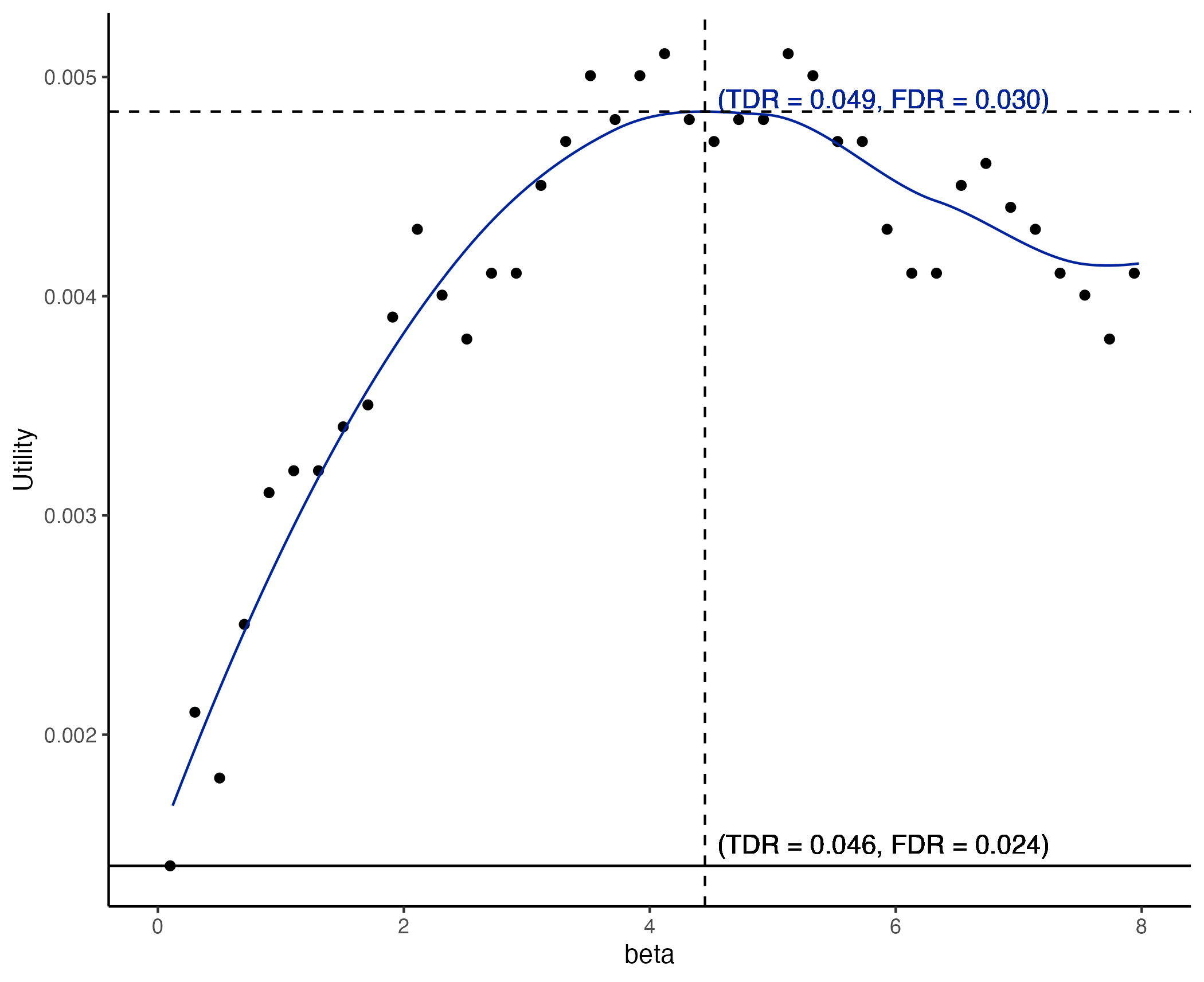
If the utility function includes large penalties for each false positive result, then , the unconstraint decision-theoretic optimum, will satisfy the regulator request of an FWER below a threshold, say . In these cases, the user of the proposed procedure can explore multiple values between zero and the regulator threshold to select the decision functions.
5.1 Results
PARP inhibitor in patients with breast cancer. The simulation study outlined in this section is motivated by our collaborative work (Tung et al.,, 2020) with investigators in breast cancer. The focus is on patients with homologous recombination (HR) defects. HR-related metastatic breast cancer is a disease setting with a median PFS of less than 24 months. Therapies that target DNA double-strand breaks, such as inhibitors of the enzyme PARP, have been successfully developed. PARP inhibitors have been shown to improve PFS, objective response rate (ORR), and quality of life compared to standard non-platinum chemotherapy in HR-related breast and ovarian cancer. Of note, the efficacy of PARP inhibitors can vary noticeably across patients with different HR alterations. Moreover, there is strong evidence that ORR is a good early surrogate of PFS improvements (Burzykowski et al.,, 2008). Our simulations consider a trial with ORR and PFS at 4 and 18 months, respectively, used as auxiliary and primary outcomes. Two subgroups are defined by gPALB2 and sBRCA1/2a mutations.
Simulation model. To evaluate the proposed approach, we conduct a simulation study with scenarios, varying the degree of correlation, and the concordance between the treatment effects on the primary and auxiliary outcomes, as follows. For each scenario, we generate RCTs with binary primary and auxiliary outcomes for () subgroups, with overall sample size . In each of these trials, the probabilities of enrolling patients from the first or second subgroup are and respectively, with expected sample sizes of and
We simulate outcome data for the experimental and control arms conditional on treatment assignments , for and using a copula model, varying the marginal outcome probabilities across scenarios, and and the odds-ratios
Simulation scenarios.
To select an appropriate method, analysts should account for context-specific considerations and compare relevant operating characteristics of alternative methods across plausible scenarios. Here, we consider scenarios with different configurations of treatment effects and correlation between primary and auxiliary outcomes. We included five configurations for the treatment effects:
1. there are no treatment effects for the primary and auxiliary outcomes in both subgroups;
2. there are no treatment effects for the primary outcome in both subgroups,
but there is a positive treatment effect for the auxiliary outcome in subgroup ;
3. there is a positive treatment effect for the primary outcome in subgroup ,
but there are no treatment effects on the auxiliary outcomes;
4. there are positive treatment effects for both the primary and auxiliary outcomes in subgroup ;
5. there is a positive treatment effect for the primary outcome in subgroup
but there is a negative treatment effect for the auxiliary outcome within the same subgroup.
For each of these five configurations, we generate data with various degrees of correlation between the primary and auxiliary outcomes. We set the marginal probability for the control arms to , and for If there is a positive treatment effect for the primary and/or auxiliary outcome, then and otherwise, the probabilities are identical to the ones for the SOC arm. For configuration 5, with a negative effect on the auxiliary outcomes (subgroup ), we set for and Finally, in our simulation scenarios, the odds-ratios are or for subgroups and arms
Hypothesis testing, utility, and decision function. The treatment effect , is the mean difference between the primary outcomes under the experimental and control therapies, and We use the parametric decision function in (6) and specify the weights for , with .
Joint Bayesian model. Prior elicitation is a key component of Bayesian design and analysis of clinical trials (e.g. Azzolina et al.,, 2021). Auxiliary and primary outcomes can be modeled jointly, and previous trials or meta-analyses can inform the prior on the unknown parameters (see Spring et al.,, 2020, for an example). We use the prior model to predict the data that the clinical trial will generate, including auxiliary and primary outcomes, and use these predictions to find the parameters of (7) that optimize the utility (5). The prior model can include information on the correlation between outcomes as well as on the correlation between the treatment effects on primary and auxiliary outcomes in previous studies. It is also important to allow for variations of the treatment effects across subgroups of patients. The prior model can be informed by previous studies, using patient-level data or summaries from completed trials. Some aspects of the model, such as the relation between treatment effects on primary and auxiliary outcomes might present substantial uncertainty, and this should be incorporated in the prior, for example, using mixtures (Schmidli et al.,, 2014).
When partial information (e.g., summary statistics) is available imputation techniques can be useful to specify a prior model for a future clinical trial (e.g., Song et al.,, 2020).
To simplify exposition, we use the same prior model for the examples considered here and in Section 6 Specifically, we use a Bayesian logistic model with correlated outcomes:
| (8) |
where is the logistic distribution function, and the independent Gaussian terms modulate the correlation between and . An advantage of model (8), compared to alternative joint models for primary and auxiliary outcomes, is that it requires a single parameter to induce correlation. This simplifies prior elicitation. We use independent normal priors for the intercepts and Their means and standard deviations, and the parameters , can be elicited from historical data. In particular, the degree of correlation between outcomes increases with the value of the subgroup-specific parameters . Therefore, the prior distribution can be elicited by matching the degree of correlation between primary and auxiliary outcomes with published estimates. Alternatively, a gamma distribution can be used as prior on . The prior for the treatment effect on the auxiliary outcome is a two-component mixture:
where is the prior probability that the experimental treatment has no effects. We then specify the prior for the treatment effect on the primary outcome conditionally on the effect on the auxiliary outcome :
where indicates the beta distribution with mean and variance . In other words, the treatment effect on the primary outcome a priori correlates with the effect on the auxiliary outcome . The values of the hyperparameters are reported in Table S1 of the Supplementary Material, together with summaries of trials generated using the prior model.
Inspecting summaries, such as the average correlation between primary and auxiliary outcomes and the correlation between treatment effects on primary and auxiliary outcomes in a subgroup of interest, is important to understand if the prior model captures well prior data from completed trials or electronic health records with sufficient uncertainty. Our prior includes different treatment effects across subgroups; for example, the prior probability of positive effects on primary outcomes in the 1st subgroup combined with the absence of positive effects in the 2nd is 1%. We also considered a variation of this prior in the Supplementary Material (see Figure S3 and Table S4).
Testing procedures. We compare the operating characteristics of the proposed procedure (indicated as Auxiliary-Augmented in Table 2) with (i) Bonferroni procedure, (ii) Holm procedure (Holm,, 1979), (iii) a testing procedure that only uses the auxiliary outcomes to evaluate the presence of treatment effects with Bonferroni corrections (Auxiliary-Only in Table 2), and (iv) an implementation of the Frequentist Assisted by Bayes (FAB) testing procedure proposed in Hoff, (2021). For all the procedures, we target an FWER Optimal parameters for the Auxiliary-Augmented procedure are illustrated in Supplementary Figure S1. We used which implies a positive utility if there is at least one true positive result. Simulations with alternative values of are discussed later in this section. The FAB procedure defines test statistics and p-values that incorporate indirect and prior information and uses a linking model; see Hoff, (2021) for details.
In our implementation of FAB, we fit logistic models for auxiliary and primary outcomes, , and We emphasize that our implementation is not consistent with the recommendations in Hoff, (2021) to include independent components of information because primary and auxiliary outcomes correlate.
Comparative simulation study. Table 2 shows for each scenario the proportion of times the null hypotheses was rejected across simulations.
In scenario 1, without positive treatment effects, all procedures control the FWER at level FAB is slightly more conservative with FWER of approximately for In scenario 2, where the auxiliary variable incorrectly indicates a positive treatment effect for group 1, the proportion of rejections of the null hypothesis is higher for the Auxiliary-Augmented procedure compared to the Bonferroni procedure (, and compared to , , and for ). However, the Auxiliary-Augmented procedure has an FWER close to the nominal level (, , and for and respectively). Also, in this scenario, FAB is slightly more conservative than the other two procedures, with FWERs of , , and for and respectively. As expected, using only the auxiliary outcomes as a surrogate for the primary outcome, the Auxiliary-Only procedure greatly inflates the FWER (, , and for and respectively) because in this scenario, there are positive effects of the treatment on the auxiliary outcome but no effects on the primary outcome.
In scenario 3, where the auxiliary outcomes incorrectly suggest no treatment effects in both subgroups, the procedures Auxiliary-Augmented, Bonferroni, and FAB perform similarly. In scenario 4, where the auxiliary variable correctly indicates the presence of a treatment effect for group 1, we observe a increase in the proportion of rejections of (true positive results) for the Auxiliary-Augmented procedure compared to the Holm and Bonferroni procedures. FAB has a lower proportion of simulation replicates that reject than the remaining procedures (e.g, compared to with Auxiliary-Augmented for ). In scenario 5, there is a positive treatment effect on the primary outcomes in subgroups but a negative effect for the auxiliary outcome in this subgroup. In this scenario, as expected, leveraging information on auxiliary treatment effects (our Auxiliary-Augmented procedure) leads to a reduction in the proportion of rejections of compared to the Holm, Bonferroni, and FAB procedures. For example, in the setting with the Auxiliary-Augmented procedure rejects with a proportion of compared to for the Holm procedure.
Sensitivity Analysis. Comparing the variations of the operating characteristics of alternative Auxiliary-Augmented procedures optimized with different values is an important sensitivity analysis. For the 15 simulation scenarios described in this section, we considered ten values of the parameter , and computed the same operating characteristics as in Table 2 . These values leads to optimal values for between and The resulting operating characteristics are reported in Table S2 of the Supplementary Material.
The FWER for simulation scenarios 1 and 2, with , is between and . In scenario 3, where the auxiliary outcomes incorrectly suggest no treatment effects in both subgroups, for increasing values of is rejected in a proportion of the simulations that varies between and , for all In scenario 4, where the auxiliary variable correctly indicates the presence of a treatment effect for group 1, is rejected in a proportion of the simulations between and
When we considered multiple values, we observed larger variations of the operating characteristic in scenario 5, with a positive treatment effect on the primary outcomes in subgroup 1 but a negative effect on the auxiliary outcome in this subgroup. In this scenario, is rejected in a proportion of the simulations between to (Table S2). As expected, with larger values of the frequency of false negative results increases.
When the subgroups have substantially different prevalences, one can consider a utility function that account for the subgroups’ prevalence. For example, it is possible to replace in the utility function (5) with multiple group-specific values (i.e., the utility becomes equal to ). Using this utility function leads to different selections of the optimal In our example, setting and that is, we increased the penalty for the first subgroup with prevalence and decreased it for the second subgroup with a prevalence of lead to the selection of
Additionally, the definition of the parametric functions used to approximate the optimal design can incorporate information on the subgroups’ prevalence. For example, one could modify (7) and redefine the weights , proportional to the product of and a monotone transformation of the -th group prevalence.
Simulation study with subgroups. Table S3 in the Supplementary Materials reports results of additional simulations with subgroups. We consider the same simulation scenarios described in this section. The data distribution for the first () subgroup is identical to the previous simulations, and the data for subgroups are generated using the same models we used for the second subgroup.
We generate RCTs for each scenario with sample size . In each of these trials, the probability that an enrolled patient belongs to the first subgroup is , and for subgroups , with an expected sample size of for the first subgroup, and for subgroups Optimal parameters for the Auxiliary-Augmented procedure are illustrated in Supplementary Figure S2. We used which implies a positive utility if the number of true positive findings is larger than the number of false positive results.
In scenarios 1 and 2, all methods present FWER close to the targeted , with the Auxiliary-Augmented procedure being slightly anti-conservative (FWER and FAB slightly conservative (FWER We note that the Auxiliary-Augmented with the the bootstrap calibration procedure described in Section 5.2 controls the FWER at the nominal level. In scenario 3, where the auxiliary outcomes incorrectly suggest no treatment effects in all the subgroups, the performance of the Auxiliary-Augmented procedure is slightly worse than the other methods. For example, with Auxiliary-Augmented rejects in of the simulation replicates compared to with the Holm procedure. In scenario 4, where the auxiliary variable correctly suggests the presence of a treatment effect for group 1, we observe a increase in the proportion of rejections of (true positive results) for Auxiliary-Augmented procedure compared to the Holm procedure. Finally, in scenario 5, where there is a positive treatment effect for the primary outcome in subgroups but a negative effect for the auxiliary outcome in the same subgroup, the performance of the Auxiliary-Augmented procedure deteriorates, as expected. The proportion of replicates with the rejection of is approximately for compared to of the Holm procedure.
| Scenario 1 | ||||||
|---|---|---|---|---|---|---|
| Method | subgroup 1 | subgroup 2 | subgroup 1 | subgroup 2 | subgroup 1 | subgroup 2 |
| Auxilary-Augmented | 0.023 | 0.029 | 0.028 | 0.029 | 0.026 | 0.023 |
| Auxilary-Augmented-B | 0.023 | 0.028 | 0.028 | 0.026 | 0.025 | 0.024 |
| Bonferroni | 0.024 | 0.028 | 0.030 | 0.030 | 0.030 | 0.028 |
| Holm | 0.025 | 0.029 | 0.029 | 0.029 | 0.027 | 0.024 |
| FAB | 0.021 | 0.022 | 0.025 | 0.021 | 0.024 | 0.019 |
| Auxiliary-Only | 0.027 | 0.026 | 0.024 | 0.028 | 0.029 | 0.025 |
| Scenario 2 | ||||||
| Method | subgroup 1 | subgroup 2 | subgroup 1 | subgroup 2 | subgroup 1 | subgroup 2 |
| Auxilary-Augmented | 0.039 | 0.014 | 0.036 | 0.017 | 0.041 | 0.019 |
| Auxilary-Augmented-B | 0.038 | 0.015 | 0.034 | 0.016 | 0.035 | 0.016 |
| Bonferroni | 0.029 | 0.025 | 0.025 | 0.025 | 0.028 | 0.026 |
| Holm | 0.029 | 0.026 | 0.026 | 0.026 | 0.029 | 0.027 |
| FAB | 0.025 | 0.018 | 0.024 | 0.020 | 0.023 | 0.022 |
| Auxiliary-Only | 0.820 | 0.026 | 0.820 | 0.029 | 0.825 | 0.026 |
| Scenario 3 | ||||||
| Method | subgroup 1 | subgroup 2 | subgroup 1 | subgroup 2 | subgroup 1 | subgroup 2 |
| Auxilary-Augmented | 0.673 | 0.026 | 0.672 | 0.031 | 0.666 | 0.036 |
| Auxilary-Augmented-B | 0.663 | 0.026 | 0.652 | 0.027 | 0.630 | 0.031 |
| Bonferroni | 0.678 | 0.027 | 0.675 | 0.029 | 0.678 | 0.031 |
| Holm | 0.682 | 0.041 | 0.678 | 0.043 | 0.683 | 0.050 |
| FAB | 0.664 | 0.019 | 0.663 | 0.022 | 0.664 | 0.023 |
| Auxiliary-Only | 0.024 | 0.030 | 0.027 | 0.027 | 0.028 | 0.028 |
| Scenario 4 | ||||||
| Method | subgroup 1 | subgroup 2 | subgroup 1 | subgroup 2 | subgroup 1 | subgroup 2 |
| Auxilary-Augmented | 0.731 | 0.014 | 0.735 | 0.019 | 0.731 | 0.016 |
| Auxilary-Augmented-B | 0.726 | 0.012 | 0.715 | 0.017 | 0.701 | 0.015 |
| Bonferroni | 0.681 | 0.022 | 0.677 | 0.031 | 0.676 | 0.024 |
| Holm | 0.683 | 0.039 | 0.680 | 0.048 | 0.679 | 0.045 |
| FAB | 0.669 | 0.017 | 0.662 | 0.024 | 0.665 | 0.018 |
| Auxiliary-Only | 0.825 | 0.029 | 0.814 | 0.024 | 0.812 | 0.025 |
| Scenario 5 | ||||||
| Method | subgroup 1 | subgroup 2 | subgroup 1 | subgroup 2 | subgroup 1 | subgroup 2 |
| Auxilary-Augmented | 0.579 | 0.037 | 0.565 | 0.041 | 0.569 | 0.043 |
| Auxilary-Augmented-B | 0.574 | 0.035 | 0.552 | 0.038 | 0.538 | 0.037 |
| Bonferroni | 0.683 | 0.026 | 0.673 | 0.029 | 0.676 | 0.028 |
| Holm | 0.686 | 0.040 | 0.676 | 0.045 | 0.678 | 0.044 |
| FAB | 0.671 | 0.020 | 0.660 | 0.019 | 0.661 | 0.022 |
| Auxiliary-Only | 0.000 | 0.029 | 0.000 | 0.028 | 0.000 | 0.026 |
5.2 Bootstrap calibration of the decision function
Proposition 2 states that for any parametrization of the decision function, the Auxiliary-Augmented testing procedure controls the FWER asymptotically at level . For RCTs with small sample sizes and strong correlations between and , the finite sample FWER might be above the nominal level, see Supplementary Figure S4 for an example. Intuitively, if the statistics and present a positive correlation, then positive values will be associated with small p-value () for the group and large weights . This mechanism can inflate the FWER.
With small sample sizes, we can estimate the FWER through simulations by generating correlated p-values () and weights in the absence of treatment effects on the primary outcome. We can use this estimation-based (bootstrap) strategy to correct for potential inflations of the FWER above the targeted value.
In particular, we use a parametric bootstrap algorithm to estimate and calibrate the FWER of the optimal parametric decision rule. For simplicity, we use instead of for the parameter of the optimal parametric decision in (see expression 4). We calibrate the testing procedure by estimating the threshold , that match the FWER of the adjusted decision functions , with the nominal -level.
We describe the calibration procedure.
Input:
-
(i)
auxiliary treatment effect estimate .
-
(ii)
estimated covariance matrices of the random vectors for .
-
(iii)
parameter .
Procedure:
-
1.
Generate data summaries .
-
2.
For each and compute the weights and the p-values , which are functions of and .
-
3.
Set , where
-
4.
Conduct the hypothesis tests using the actual data and ,
The input parameters can be set using any consistent estimator of the treatment effects and covariance matrices such as maximum likelihood or Bayesian estimates. Figure S4 shows that the outlined bootstrap calibration algorithm controls the FWER at the nominal -level. Moreover, for small odds ratios () we observe minor reductions in power of approximately ; with the power reductions are approximately (see scenarios 3-4 in Table 2).
6 Auxiliary outcomes for interim decisions in RCTs
Motivation. We discuss a multi-stage design motivated by our work in newly diagnosed glioblastoma (nGBM) (Vanderbeek et al.,, 2018, 2019), an aggressive form of brain cancer. The SOC in nGBM is temozolomide in combination with radiation therapy (TMZ+RT), which was approved more than 15 years ago based on the results of the EORTC-NCIC CE.3 trial (Stupp et al.,, 2005). Clinical outcomes remain poor, with a median overall survival of less than months. All confirmatory phase III RCTs since 2005 failed to demonstrate OS improvements compared to TMZ+RT. Several primary and co-primary outcomes have been used in recent nGBM trials (e.g., ORR, OS, PFS, and OS at 24 months).
Investigators in nGBM have pointed to the need for novel drug development strategies and effective trial designs capable of rapidly discontinuing the evaluation of toxic or inferior experimental treatments without compromising the power (e.g., Ventz et al.,, 2021). Several authors proposed prediction procedures that trigger futility-stopping decisions, and some of the resulting approaches are applied in current clinical research.
We hypothesize that combining information on primary and auxiliary outcomes can improve interim decision-making and expose fewer patients to experimental treatments without positive effects. Additionally, with improved interim predictions, the power of the study can increase by reducing the likelihood of early stopping for futility when the experimental treatment has a positive effect on the primary outcome. Recent contributions have shown that early auxiliary outcomes, which are predictive of the primary outcomes, can be useful to estimate the conditional power (Qing et al.,, 2022; Li et al.,, 2023). The use of surrogate or auxiliary outcomes to predict if a future RCT will demonstrate positive effects on the primary outcome has also been previously discussed; see for example Saint-Hilary et al., (2019). Here, we leverage primary and auxiliary outcomes to make early futility decisions during the trial according to explicit utility criteria.
We consider a group-sequential trial design (Demets and Lan,, 1994) that uses overall survival after 18 months of treatment (OS-18, ) as primary outcome, and ORR () according to the iRANO criteria (Wen et al.,, 2010) as auxiliary outcome.
Study design. The trial design includes stages and evaluates efficacy in the overall population (i.e., ), with a maximum of interim decisions based on available evidence for futility or efficacy. The design also includes a potential efficacy test at the end of the trial (i.e., ). In particular, each IA can (i) reject the null hypothesis of no treatment effect on the primary outcome if there is sufficient early evidence and close the study, (ii) terminate the trial early for futility if additional data are unlikely to demonstrate positive effects of the experimental treatment on the primary outcomes, or (iii) continue the study. At the end of the -th stage (), the design includes an efficacy analysis, followed by a futility analysis unless was rejected. The -th analysis occurs after the primary outcomes of the first patients become available, exactly 18 months after the enrollment of the -th patient, where are fixed design parameters. Potentially more than auxiliary outcomes are available at IA and are used for interim decisions. Lastly, we use to indicate the number of enrollments before the -th analysis.
Frequentist constraint and utility function. The type I error rate is controlled at level . We indicate with , , the efficacy decisions and with , , the futility decisions. Let be the time when the trial stops. We use the utility function
| (9) |
with and , for . This utility function assigns a reward for correctly rejecting the null hypothesis at time if the treatment prolong survival, and a cost for each enrolled patient.
Parametric efficacy decision function. There are several popular sequential decision rules to stop a trial for efficacy, including the Pocock (Pocock,, 1977) and O’Brien–Fleming (O’Brien and Fleming,, 1979) stopping rules, and the alpha-spending functions approach (Gordon Lan and Demets,, 1983). We specify the efficacy stopping rule , which will be parameterized by using an alpha-spending function (Gordon Lan and Demets,, 1983). Early stopping for efficacy leverages only primary outcomes. For binary outcomes, the alpha-spending function for is a function of the information fraction It determines the proportion of the overall type I error rate that is spent by the -th IA. The type-I error allocated to the -th IA is - , where we refer to Gordon Lan and Demets, (1983) and Demets and Lan, (1994) for details. We use the one-parameter family introduced in Hwang et al., (1990):
| (10) |
for .
As in Section 5, we use efficacy decisions based on Z-statistics. Let be the -statistics based on the primary outcomes of the first patients. We indicate with the recursively defined -quantiles of the conditional distributions , where is a mean zero Gaussian vector with covariance for . The resulting values are the Z-statistics thresholds for the efficacy decisions (i.e., ). See Jennison and Turnbull, (1999) for a detailed explanation of how to compute the vector
Parametric futility decision function. Several approaches for early futility stopping propose rules to stop the trial at IA if, given the available interim data, the likelihood of obtaining a statistically significant study result at any stage falls below a pre-defined threshold (Lan et al.,, 1982; Betensky,, 1997; Lachin,, 2005; Berry et al.,, 2010). The likelihood of a positive result can be computed using frequentist (Lan et al.,, 1982; Betensky,, 1997; Lachin,, 2005) or Bayesian methodologies (Spiegelhalter et al.,, 1986; Berry et al.,, 2010). Most of these methods approximate the probability through computations that ignore the possibility of stopping for futility at time , that is all future futility IAs are ignored. We specify the futility stopping criteria (i.e., ) using Bayesian modeling. Our approach leverages auxiliary and primary outcomes into predictions and futility decisions. We stop for futility , when . Note that is parametrized by The conditional probability that we use for futility decisions, is based on a joint model of primary and auxiliary outcomes. We compute these probabilities using the Hamiltonian Monte Carlo implemented in rstan (Stan Development Team,, 2023).
Prior model. We use the same prior model as in Section 5 with . Optimal values for are obtained by maximizing the utility (9), with , and a cost of for each patient. See also Supplementary Figure S5 for details.
Simulation Scenarios. We consider a two-stage RCT () with a maximum sample size of and We use the same model as in Section 5.1 with to generate the data, and use the same simulation scenarios (population ) as in Section 5.1.
Alternative trial designs. We compare our approach (Auxiliary-Augmented in Table 3) with two alternative trial designs. The first is the Primary-Only design, which uses only the primary outcome data for efficacy and futility analyses. This design uses the same group-sequential efficacy rule as the Auxiliary-Augmented design, which is based on a -spending (10) with . The futility decisions are based on a Bayesian model that ignores auxiliary information, a variation of model (8). Specifically, we use the model with a Gaussian prior on , and the mixture for We use the same futility threshold of the Auxiliary-Augmented design. The other design in our comparisons is the Auxiliary-Only design. It is nearly identical to the Primary-Only design, but it replaces the primary outcomes with the auxiliary outcomes for efficacy and futility decisions.
Results. Table 3 summarizes our simulation results. For each scenario, we report the proportion of simulations in which the null hypothesis of no treatment effects is rejected. We also report the frequency of simulations in which is rejected at IA and FA, and the average sample size. In these trial simulations, we did not model the patient enrollment times.
In scenario 1, without positive treatment effects, the three designs control the type-I error at The Auxiliary-Augmented design has the lowest expected sample size with approximatively patients compared to and of the Primary-Only and Auxiliary-Only designs.
In scenario 2, the auxiliary outcomes suggest a positive effect, but the experimental therapy does not improve survival. Not surprisingly, the Auxiliary-Only design has a highly inflated type-I error rate. The Auxiliary-Augmented and Primary-Only designs control the type I error at the nominal level. In these simulations, the Auxiliary-Augmented design, as expected, stops the trial for futility less frequently than the Primary-Only design; the resulting average sample sizes are and patients.
In scenario 3, there is a positive effect on survival, but the effect on the auxiliary outcomes is null. The Auxilairy-Only design does not detect the treatment effect; the power is . The Primary-Only design has a power of and an expected sample size of approximatively patients, compared to the Auxiliary-Augmented design with a power of approximately and an average sample size of patients.
In scenario 4, there is a positive treatment effect on both primary and auxiliary outcomes. The Auxiliary-Only design has a power of approximately and an average sample size of patients. In comparison, the Primary-Only design has a power of and an average sample size of patients, and the Auxiliary-Augmented design has a power of with an average sample size of patients.
In scenario 5, there is a positive effect on the primary outcome and a negative effect on the auxiliary. The Auxiliary-Only design does not detect the treatment effect. The Primary-Only design has a power of approximately and an average sample size of patients, while the Auxiliary-Augmented design, as expected, presents a reduced power of approximately , due to early futility decisions, and an average sample size of patients.
| Scenario 1 | ||||||
|---|---|---|---|---|---|---|
| Design | False positive results | False positive results | False positive results | |||
| Auxiliary-Augmented | 0.048 (0.042; 0.006) | 107.6 | 0.043 (0.036; 0.008) | 108.3 | 0.051 (0.042; 0.009) | 109.2 |
| Primary-Only | 0.054 (0.043; 0.011) | 118.2 | 0.049 (0.036; 0.013) | 117.8 | 0.055 (0.043; 0.012) | 118.4 |
| Auxiliary-Only | 0.060 (0.046; 0.014) | 126.7 | 0.047 (0.038; 0.010) | 125.9 | 0.057 (0.041; 0.015) | 128.3 |
| Scenario 2 | ||||||
| Design | False positive results | False positive results | False positive results | |||
| Auxiliary-Augmented | 0.055 (0.039; 0.016) | 137.5 | 0.055 (0.039; 0.015) | 136.9 | 0.053 (0.039; 0.014) | 138.1 |
| Primary-Only | 0.053 (0.039; 0.014) | 118.2 | 0.052 (0.039; 0.012) | 117.6 | 0.051 (0.039; 0.013) | 118.8 |
| Auxiliary-Only | 0.958 (0.791; 0.167) | 119.6 | 0.956 (0.788; 0.168) | 119.6 | 0.961 (0.792; 0.169) | 119.5 |
| Scenario 3 | ||||||
| Design | Power | Power | Power | |||
| Auxiliary-Augmented | 0.788 (0.661; 0.126) | 116.5 | 0.797 (0.661; 0.137) | 117.0 | 0.791 (0.677; 0.114) | 113.6 |
| Primary-Only | 0.866 (0.664; 0.202) | 127.6 | 0.873 (0.664; 0.209) | 127.9 | 0.873 (0.680; 0.194) | 125.9 |
| Auxiliary-Only | 0.052 (0.040; 0.013) | 127.5 | 0.051 (0.040; 0.012) | 178.1 | 0.053 (0.039; 0.014) | 129.1 |
| Scenario 4 | ||||||
| Design | Power | Power | Power | |||
| Auxiliary-Augmented | 0.892 (0.673; 0.219) | 130.7 | 0.887 (0.666; 0.221) | 130.9 | 0.892 (0.666; 0.226) | 130.5 |
| Primary-Only | 0.876 (0.673; 0.204) | 126.9 | 0.870 (0.666; 0.204) | 127.4 | 0.876 (0.666; 0.210) | 127.4 |
| Auxiliary-Only | 0.959 (0.805; 0.154) | 118.3 | 0.961 (0.790; 0.170) | 119.6 | 0.962 (0.789; 0.173) | 120.2 |
| Scenario 5 | ||||||
| Design | Power | Power | Power | |||
| Auxiliary-Augmented | 0.519 (0.511; 0.008) | 101.0 | 0.540 (0.533; 0.008) | 101.0 | 0.519 (0.514; 0.006) | 100.6 |
| Primary-Only | 0.877 (0.668; 0.209) | 127.1 | 0.876 (0.678; 0.198) | 126.5 | 0.868 (0.663; 0.205) | 127.4 |
| Auxiliary-Only | 0.000 (0.000; 0.000) | 100.1 | 0.000 (0.000; 0.000) | 100.1 | 0.000 (0.000; 0.000) | 100.1 |
6.1 Retrospective analysis with GBM trial data
We use patient-level data from the CENTRIC trial (Stupp et al.,, 2014) to evaluate the Auxiliary-Augmented trial design. The CENTRIC study was a large Phase 3 clinical trial that enrolled patients with nGBM and tumors with methylated O6-methylguanine (MGMT). The data on the patients treated with the SOC (TMZ+RT) that we used are available through Project Data Sphere (https://data.projectdatasphere.org/). We have patients treated with TMZ+RT. Our analysis uses overall survival at 24 months (OS-24) as the binary primary outcome and progression-free survival at 12 months (PFS-12) as auxiliary outcome. We excluded patients with unknown 24-month survival status from the analysis.
We consider an RCT with a control arm (TMZ+RT) and an experimental arm, a total sample size of patients and one interim analysis. The target type-I error is To determine the optimal values , we used the same prior and utility functions of the previous simulation.
To generate in silico trial replicates tailored to nGBM, we follow these two steps:
-
1.
We sample with replacement a patient from the TMZ+RT group of the CENTRIC dataset. The patient is randomly assigned to either the TMZ+RT or the experimental arm of our in silico trial.
-
2.
If the patient is assigned to our in silico TMZ+RT, we include the actual OS-24 and PFS-12 as primary and auxiliary outcomes. If the patient is assigned to the in silico experimental arm, we use a simple and interpretable perturbation of the actual OS-24 and PFS-12 to produce scenarios with positive or negative treatment effects. If the actual outcome was negative, we relabel the individual primary outcome into positive with probability . Similarly, we relabel a negative auxiliary outcome into a positive with probability . The parameters and create in silico trials with treatment effects.
By adjusting the values of and , we create scenarios to examine the trial design, with or without concordance of the treatment effects on primary and auxiliary outcomes. We considered three scenarios: 1. (null scenario) there are no treatment effects on both primary and auxiliary outcome; 2. (concordant effects) and ; 3. (discordant effects) and mimicking a trial where an effect is present for PFS but not on OS. We mention, as an example, the study of lomustine and bevacizumab (Wick et al.,, 2017), in which the effects on primary and auxiliary outcomes were discordant.
In our analysis, we compared the Auxiliary-Augmented, Primary-Only, and Auxiliary-Only designs. In our in silico trials, we did not model the individual enrollment times.
| Scenario 1 | Scenario 2 | Scenario 3 | ||||
|---|---|---|---|---|---|---|
| null scenario | concordant effects | discordant effects | ||||
| Method | Power | Power | Power | |||
| Auxiliary-Augmented | 0.050 (0.041; 0.009) | 113.8 | 0.809 (0.556; 0.253) | 142.0 | 0.052 (0.041; 0.011) | 151.6 |
| Primary-Only | 0.051 (0.041; 0.010) | 127.9 | 0.798 (0.556; 0.241) | 138.2 | 0.051 (0.041; 0.010) | 128.2 |
| Auxiliary-Only | 0.047 (0.037; 0.010) | 125.8 | 0.988 (0.881; 0.107) | 111.4 | 0.987 (0.877; 0.110) | 111.7 |
Table 4 summarizes the results. In scenario 1, without treatment effects, all three designs control the type-I error at the The Auxiliary-Augmented design has the lowest average sample size with patients, compared to 128 for the Primary-Only design, and for the Auxiliary-Only design. In scenario 2, with treatment effects both on primary and auxiliary outcomes, the Auxiliary-Only design has an average sample size of 142 patients (81% power) compared to patients (80% power) for the Primary-Only design, and (99% power) for the Auxiliary-Only design. In scenario 3, with a treatment effect only on the auxiliary outcomes, as expected, the Auxiliary-Only design has an inflated type-I error, while the Auxiliary-Augmented and Auxiliary-Only designs control the type-I error at Due to promising auxiliary data, the Auxiliary-Augmented design has an average sample size of patients compared to of the Auxiliary-Only design.
In Section S2 of the Supplementary Material we re-implement this retrospective analysis using time-to-event outcomes.
7 Discussion
Demonstrating OS improvements with experimental therapies is typically the ultimate and most clinically relevant goal in oncology research. Nonetheless, early outcomes, including tumor response and radiographic measures, are extensively used in clinical trials (Delgado and Guddati,, 2021). Direct use of early outcomes as surrogates of OS throughout the drug development process presents potential efficiencies and risks. Discordant treatment effects on early outcomes and OS have been repeatedly discussed in the oncology literature, with several cases of promising results on early outcomes in the initial phases of drug development that are followed by negative results of large phase III trials assessing the drug effects on OS (Merino et al.,, 2023). In this paper, we discuss a new approach to making decisions during the drug development process that is based on joint analyses of primary and auxiliary outcomes. The proposed method allows the enforcement of frequentist operating characteristics aligned with the requests of the regulator or other stakeholders’ needs. For example, when we consider RCTs that test treatments in several subgroups and control FWER, our approach leads to a substantial gain in efficiency compared to standard methods that exclude the auxiliary data from the analyses.
When auxiliary variables are integrated into interim and final analyses of clinical studies, it is important to balance potential benefits associated with early signals of efficacy, available in a short period of time, and risks (e.g., planning a large phase III trial based on promising auxiliary data but without evidence of positive effects on the primary outcomes). We focus on this trade-off formalized by the maximization of explicit utility criteria representative of the aims of the clinical trial and frequentist constraints that appropriately control the risks of the trial. Decision-theoretic approaches that combine Bayesian modeling, explicit utility functions, and frequentist constraints are useful for the design and analysis of clinical trials (Ventz and Trippa,, 2015; Arfè et al.,, 2020). The use of prior models is particularly attractive in settings where the analyst has access to collections of real-world data and completed trials. A key feature of our approach is the use of simple and easy-to-interpret decision functions that incorporate treatment effects estimates for the primary and auxiliary outcomes. As outlined in Section 4, these parametric decision functions allow us to combine data on primary and auxiliary outcomes. In our experience, parametric decision functions are computationally attractive because they allow the user to restrict the space of candidate designs to reasonable and easy-to-describe subsets.
The proposed framework can be applied to several decision problems, including complex designs with a combination of interim decisions, multi-group, and multiple treatment arms. As an example, we can consider clinical studies that attempt to identify subgroups of patients in which the experimental treatment has positive effects. With many candidate partitions of the population, there is the risk of cherry-picking the most promising subgroups (Guo and He,, 2021). In this example, auxiliary and primary outcomes could be used to select and recommend subgroups for subsequent confirmatory trials. In particular, an interpretable utility function can mirror the number of patients who will benefit from the treatment after regulatory approval. Meanwhile, frequentist constraints can bound the probability that the phase III confirmatory study fails to demonstrate the efficacy of the experimental therapy. In summary, the approach combines auxiliary and primary outcomes to identify subgroups while controlling the risk of a subsequent phase III trial failure.
Acknowledgments
The examples in Section 6.1 and Supplementary Section S2 are based on research using information obtained from www.projectdatasphere.org, which is maintained by Project Data Sphere. Neither Project Data Sphere nor the owner(s) of any information from the website have contributed to, approved, or are in any way responsible for the contents of this publication. Lorenzo Trippa and Steffen Ventz have been supported by the NIH grant R01LM013352.
Supplementary Material
S1 Supplementary figures and tables
Code to reproduce figures and tables is available at https://github.com/rMassimiliano/primary_and_auxiliary.
| Mean | Min. | 1st Qu. | Median | 3rd Qu. | Max. | |
|---|---|---|---|---|---|---|
| Proportion Y=1 (SOC) | 0.238 | 0.029 | 0.175 | 0.230 | 0.294 | 0.657 |
| Proportions Y=1 (Treated) | 0.242 | 0.017 | 0.176 | 0.231 | 0.299 | 0.76 2 |
| Difference in proportions (TE) for Y | 0.003 | -0.236 | -0.038 | 0.002 | 0.044 | 0.289 |
| Proportion S=1 (SOC) | 0.349 | 0.069 | 0.276 | 0.344 | 0.416 | 0.764 |
| Proportions S=1 (Treated) | 0.352 | 0.039 | 0.274 | 0.347 | 0.424 | 0.81 4 |
| Difference in proportions (TE) for S | 0.003 | -0.380 | -0.046 | 0.002 | 0.050 | 0.342 |
| Correlation between Y and S | 0.138 | -0.197 | 0.085 | 0.138 | 0.193 | 0 .414 |
| Scenario 1 | ||||||||||
|---|---|---|---|---|---|---|---|---|---|---|
| ( | (0.1, 14.07) | (0.2, 13.91) | (0.3, 13.75) | (0.4, 13.43) | (0.5, 4.45) | (0.6, 4.21) | (0.7, 4.05) | (0.8, 3.93) | (0.9, 3.81) | (1.0, 3.69) |
| subgroup 1 | 0.022 | 0.022 | 0.022 | 0.022 | 0.023 | 0.023 | 0.023 | 0.023 | 0.023 | 0.023 |
| subgroup 2 | 0.029 | 0.029 | 0.029 | 0.029 | 0.029 | 0.029 | 0.029 | 0.029 | 0.029 | 0.029 |
| Scenario 1 | ||||||||||
| ( | (0.1, 14.07) | (0.2, 13.91) | (0.3, 13.75) | (0.4, 13.43) | (0.5, 4.45) | (0.6, 4.21) | (0.7, 4.05) | (0.8, 3.93) | (0.9, 3.81) | (1.0, 3.69) |
| subgroup 1 | 0.030 | 0.030 | 0.030 | 0.030 | 0.030 | 0.030 | 0.030 | 0.030 | 0.030 | 0.030 |
| subgroup 2 | 0.031 | 0.031 | 0.031 | 0.031 | 0.031 | 0.030 | 0.030 | 0.030 | 0.030 | 0.030 |
| Scenario 1 | ||||||||||
| ( | (0.1, 14.07) | (0.2, 13.91) | (0.3, 13.75) | (0.4, 13.43) | (0.5, 4.45) | (0.6, 4.21) | (0.7, 4.05) | (0.8, 3.93) | (0.9, 3.81) | (1.0, 3.69) |
| subgroup 1 | 0.032 | 0.032 | 0.032 | 0.032 | 0.030 | 0.030 | 0.030 | 0.030 | 0.030 | 0.030 |
| subgroup 2 | 0.033 | 0.033 | 0.033 | 0.033 | 0.028 | 0.028 | 0.028 | 0.028 | 0.028 | 0.028 |
| Scenario 2 | ||||||||||
| ( | (0.1, 14.07) | (0.2, 13.91) | (0.3, 13.75) | (0.4, 13.43) | (0.5, 4.45) | (0.6, 4.21) | (0.7, 4.05) | (0.8, 3.93) | (0.9, 3.81) | (1.0, 3.69) |
| subgroup 1 | 0.047 | 0.047 | 0.047 | 0.046 | 0.039 | 0.039 | 0.038 | 0.038 | 0.038 | 0.037 |
| subgroup 2 | 0.004 | 0.005 | 0.005 | 0.005 | 0.014 | 0.015 | 0.015 | 0.016 | 0.016 | 0.016 |
| Scenario 2 | ||||||||||
| ( | (0.1, 14.07) | (0.2, 13.91) | (0.3, 13.75) | (0.4, 13.43) | (0.5, 4.45) | (0.6, 4.21) | (0.7, 4.05) | (0.8, 3.93) | (0.9, 3.81) | (1.0, 3.69) |
| subgroup 1 | 0.044 | 0.043 | 0.043 | 0.043 | 0.036 | 0.036 | 0.036 | 0.035 | 0.035 | 0.035 |
| subgroup 2 | 0.008 | 0.008 | 0.008 | 0.009 | 0.017 | 0.017 | 0.018 | 0.018 | 0.018 | 0.018 |
| Scenario 2 | ||||||||||
| ( | (0.1, 14.07) | (0.2, 13.91) | (0.3, 13.75) | (0.4, 13.43) | (0.5, 4.45) | (0.6, 4.21) | (0.7, 4.05) | (0.8, 3.93) | (0.9, 3.81) | (1.0, 3.69) |
| subgroup 1 | 0.050 | 0.050 | 0.050 | 0.050 | 0.041 | 0.040 | 0.039 | 0.039 | 0.039 | 0.038 |
| subgroup 2 | 0.010 | 0.010 | 0.010 | 0.010 | 0.019 | 0.020 | 0.020 | 0.020 | 0.020 | 0.020 |
| Scenario 3 | ||||||||||
| ( | (0.1, 14.07) | (0.2, 13.91) | (0.3, 13.75) | (0.4, 13.43) | (0.5, 4.45) | (0.6, 4.21) | (0.7, 4.05) | (0.8, 3.93) | (0.9, 3.81) | (1.0, 3.69) |
| subgroup 1 | 0.625 | 0.627 | 0.627 | 0.628 | 0.673 | 0.673 | 0.673 | 0.673 | 0.673 | 0.674 |
| subgroup 2 | 0.027 | 0.027 | 0.027 | 0.027 | 0.026 | 0.027 | 0.027 | 0.027 | 0.027 | 0.027 |
| Scenario 3 | ||||||||||
| ( | (0.1, 14.07) | (0.2, 13.91) | (0.3, 13.75) | (0.4, 13.43) | (0.5, 4.45) | (0.6, 4.21) | (0.7, 4.05) | (0.8, 3.93) | (0.9, 3.81) | (1.0, 3.69) |
| subgroup 1 | 0.631 | 0.631 | 0.631 | 0.635 | 0.673 | 0.673 | 0.673 | 0.674 | 0.674 | 0.674 |
| subgroup 2 | 0.030 | 0.030 | 0.030 | 0.030 | 0.031 | 0.031 | 0.031 | 0.031 | 0.030 | 0.031 |
| Scenario 3 | ||||||||||
| ( | (0.1, 14.07) | (0.2, 13.91) | (0.3, 13.75) | (0.4, 13.43) | (0.5, 4.45) | (0.6, 4.21) | (0.7, 4.05) | (0.8, 3.93) | (0.9, 3.81) | (1.0, 3.69) |
| subgroup 1 | 0.618 | 0.619 | 0.620 | 0.621 | 0.666 | 0.666 | 0.667 | 0.667 | 0.668 | 0.669 |
| subgroup 2 | 0.042 | 0.042 | 0.041 | 0.042 | 0.036 | 0.036 | 0.036 | 0.035 | 0.035 | 0.035 |
| Scenario 4 | ||||||||||
| ( | (0.1, 14.07) | (0.2, 13.91) | (0.3, 13.75) | (0.4, 13.43) | (0.5, 4.45) | (0.6, 4.21) | (0.7, 4.05) | (0.8, 3.93) | (0.9, 3.81) | (1.0, 3.69) |
| subgroup 1 | 0.757 | 0.757 | 0.757 | 0.757 | 0.731 | 0.729 | 0.727 | 0.727 | 0.726 | 0.725 |
| subgroup 2 | 0.006 | 0.006 | 0.006 | 0.006 | 0.014 | 0.013 | 0.013 | 0.013 | 0.014 | 0.014 |
| Scenario 4 | ||||||||||
| ( | (0.1, 14.07) | (0.2, 13.91) | (0.3, 13.75) | (0.4, 13.43) | (0.5, 4.45) | (0.6, 4.21) | (0.7, 4.05) | (0.8, 3.93) | (0.9, 3.81) | (1.0, 3.69) |
| subgroup 1 | 0.760 | 0.759 | 0.759 | 0.759 | 0.735 | 0.733 | 0.732 | 0.731 | 0.728 | 0.728 |
| subgroup 2 | 0.008 | 0.008 | 0.008 | 0.009 | 0.018 | 0.019 | 0.020 | 0.021 | 0.021 | 0.021 |
| Scenario 4 | ||||||||||
| ( | (0.1, 14.07) | (0.2, 13.91) | (0.3, 13.75) | (0.4, 13.43) | (0.5, 4.45) | (0.6, 4.21) | (0.7, 4.05) | (0.8, 3.93) | (0.9, 3.81) | (1.0, 3.69) |
| subgroup 1 | 0.763 | 0.763 | 0.763 | 0.763 | 0.731 | 0.729 | 0.728 | 0.727 | 0.726 | 0.724 |
| subgroup 2 | 0.011 | 0.011 | 0.011 | 0.011 | 0.016 | 0.016 | 0.016 | 0.017 | 0.017 | 0.018 |
| Scenario 5 | ||||||||||
| ( | (0.1, 14.07) | (0.2, 13.91) | (0.3, 13.75) | (0.4, 13.43) | (0.5, 4.45) | (0.6, 4.21) | (0.7, 4.05) | (0.8, 3.93) | (0.9, 3.81) | (1.0, 3.69) |
| subgroup 1 | 0.338 | 0.341 | 0.344 | 0.352 | 0.578 | 0.586 | 0.590 | 0.592 | 0.595 | 0.598 |
| subgroup 2 | 0.044 | 0.044 | 0.044 | 0.044 | 0.037 | 0.036 | 0.036 | 0.036 | 0.036 | 0.036 |
| Scenario 5 | ||||||||||
| ( | (0.1, 14.07) | (0.2, 13.91) | (0.3, 13.75) | (0.4, 13.43) | (0.5, 4.45) | (0.6, 4.21) | (0.7, 4.05) | (0.8, 3.93) | (0.9, 3.81) | (1.0, 3.69) |
| subgroup 1 | 0.336 | 0.339 | 0.343 | 0.349 | 0.564 | 0.572 | 0.577 | 0.581 | 0.584 | 0.587 |
| subgroup 2 | 0.050 | 0.050 | 0.050 | 0.050 | 0.041 | 0.041 | 0.040 | 0.040 | 0.040 | 0.039 |
| Scenario 5 | ||||||||||
| ( | (0.1, 14.07) | (0.2, 13.91) | (0.3, 13.75) | (0.4, 13.43) | (0.5, 4.45) | (0.6, 4.21) | (0.7, 4.05) | (0.8, 3.93) | (0.9, 3.81) | (1.0, 3.69) |
| subgroup 1 | 0.337 | 0.339 | 0.341 | 0.349 | 0.568 | 0.574 | 0.578 | 0.582 | 0.585 | 0.588 |
| subgroup 2 | 0.050 | 0.050 | 0.050 | 0.050 | 0.043 | 0.042 | 0.042 | 0.042 | 0.042 | 0.042 |
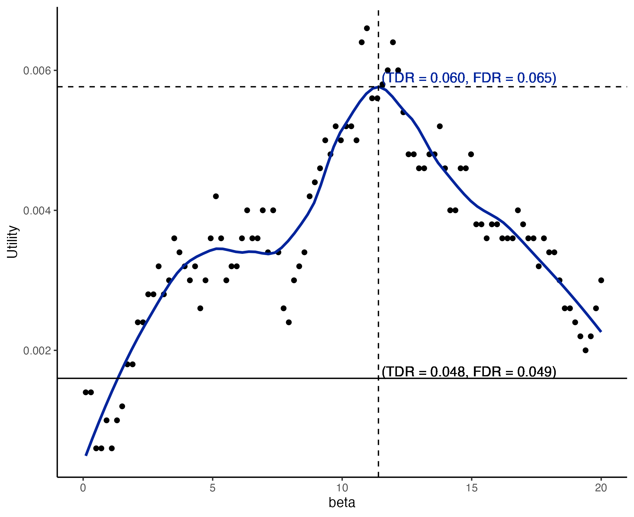
| Scenario 1 | ||||||
|---|---|---|---|---|---|---|
| Method | subgroup 1 | subgroup 2–6 | subgroup 1 | subgroup 2–6 | subgroup 1 | subgroup 2–6 |
| Auxiliary-Augmented | 0.009 | 0.048 | 0.009 | 0.051 | 0.009 | 0.048 |
| Auxiliary-Augmented-B | 0.009 | 0.046 | 0.007 | 0.051 | 0.006 | 0.041 |
| Bonferroni | 0.010 | 0.044 | 0.010 | 0.066 | 0.012 | 0.079 |
| Holm | 0.010 | 0.044 | 0.009 | 0.051 | 0.009 | 0.048 |
| FAB | 0.007 | 0.023 | 0.007 | 0.029 | 0.007 | 0.026 |
| Auxiliary-Only | 0.013 | 0.048 | 0.009 | 0.050 | 0.010 | 0.047 |
| Scenario 2 | ||||||
| Method | subgroup 1 | subgroup 2–6 | subgroup 1 | subgroup 2–6 | subgroup 1 | subgroup 2–6 |
| Auxiliary-Augmented | 0.035 | 0.022 | 0.033 | 0.028 | 0.039 | 0.043 |
| Auxiliary-Augmented-B | 0.031 | 0.023 | 0.026 | 0.020 | 0.021 | 0.023 |
| Bonferroni | 0.009 | 0.047 | 0.007 | 0.046 | 0.011 | 0.049 |
| Holm | 0.009 | 0.047 | 0.007 | 0.046 | 0.011 | 0.049 |
| FAB | 0.007 | 0.027 | 0.005 | 0.025 | 0.008 | 0.028 |
| Auxiliary-Only | 0.799 | 0.046 | 0.801 | 0.050 | 0.791 | 0.047 |
| Scenario 3 | ||||||
| Method | subgroup 1 | subgroup 2–6 | subgroup 1 | subgroup 2–6 | subgroup 1 | subgroup 2–6 |
| Auxiliary-Augmented | 0.560 | 0.047 | 0.565 | 0.061 | 0.560 | 0.085 |
| Auxiliary-Augmented-B | 0.555 | 0.045 | 0.529 | 0.046 | 0.457 | 0.037 |
| Bonferroni | 0.625 | 0.049 | 0.637 | 0.047 | 0.629 | 0.046 |
| Holm | 0.626 | 0.054 | 0.638 | 0.054 | 0.629 | 0.053 |
| FAB | 0.597 | 0.030 | 0.613 | 0.027 | 0.603 | 0.027 |
| Auxiliary-Only | 0.008 | 0.048 | 0.011 | 0.044 | 0.009 | 0.051 |
| Scenario 4 | ||||||
| Method | subgroup 1 | subgroup 2–6 | subgroup 1 | subgroup 2–6 | subgroup 1 | subgroup 2–6 |
| Auxiliary-Augmented | 0.799 | 0.019 | 0.791 | 0.032 | 0.780 | 0.046 |
| Auxiliary-Augmented-B | 0.791 | 0.019 | 0.752 | 0.025 | 0.690 | 0.024 |
| Bonferroni | 0.629 | 0.047 | 0.632 | 0.052 | 0.630 | 0.053 |
| Holm | 0.631 | 0.050 | 0.633 | 0.057 | 0.630 | 0.061 |
| FAB | 0.602 | 0.025 | 0.609 | 0.028 | 0.607 | 0.028 |
| Auxiliary-Only | 0.795 | 0.045 | 0.799 | 0.045 | 0.798 | 0.046 |
| Scenario 5 | ||||||
| Method | subgroup 1 | subgroup 2–6 | subgroup 1 | subgroup 2–6 | subgroup 1 | subgroup 2–6 |
| Auxiliary-Augmented | 0.276 | 0.058 | 0.277 | 0.067 | 0.284 | 0.089 |
| Auxiliary-Augmented-B | 0.270 | 0.053 | 0.252 | 0.053 | 0.219 | 0.048 |
| Bonferroni | 0.631 | 0.049 | 0.619 | 0.045 | 0.621 | 0.048 |
| Holm | 0.633 | 0.055 | 0.619 | 0.051 | 0.623 | 0.052 |
| FAB | 0.610 | 0.027 | 0.591 | 0.023 | 0.594 | 0.026 |
| Auxiliary-Only | 0.000 | 0.050 | 0.000 | 0.045 | 0.000 | 0.051 |
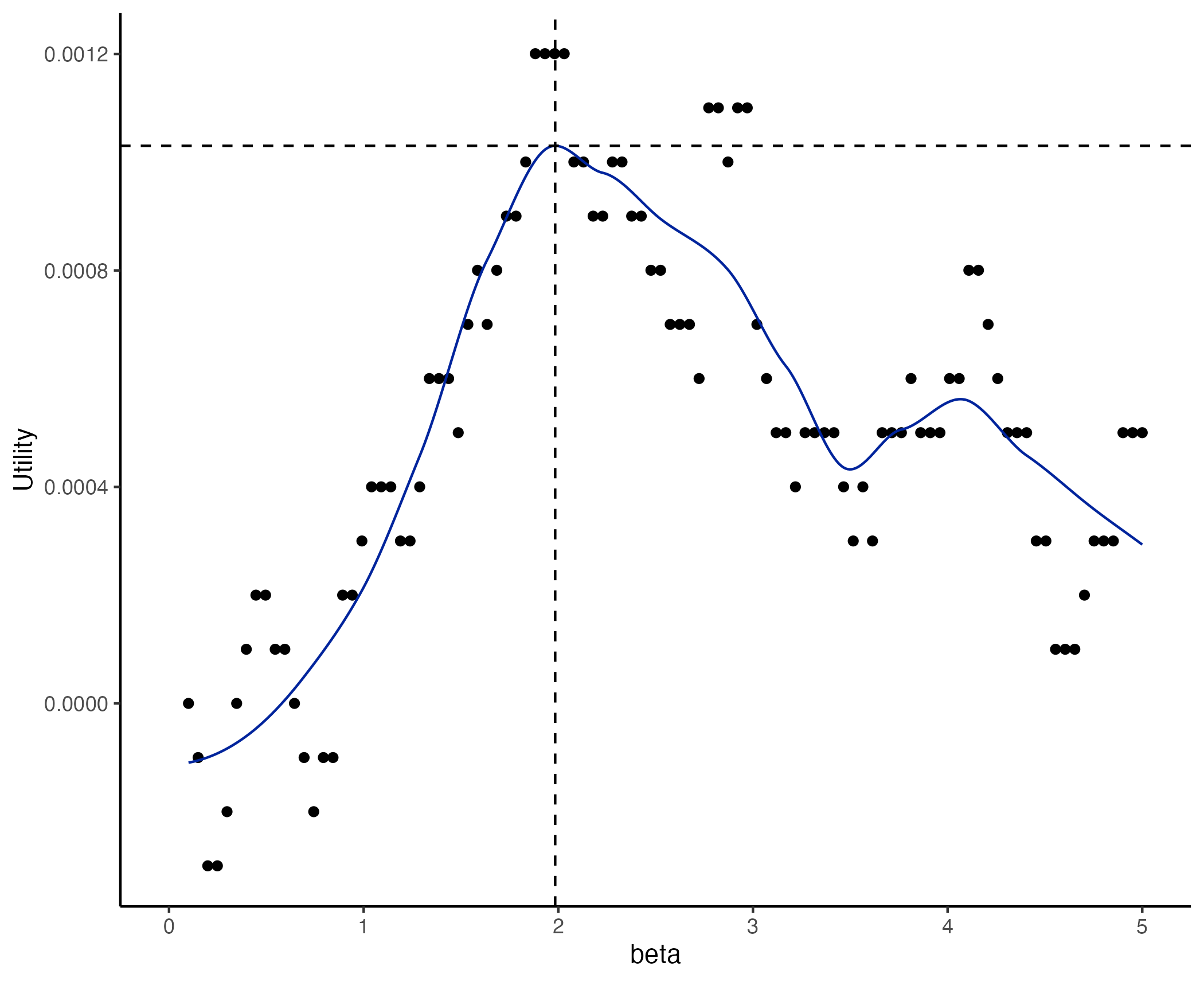
| Scenario 1 | 0.023 | 0.027 | 0.029 | 0.028 | 0.028 | 0.026 |
|---|---|---|---|---|---|---|
| Scenario 2 | 0.034 | 0.020 | 0.031 | 0.022 | 0.033 | 0.022 |
| Scenario 3 | 0.677 | 0.027 | 0.679 | 0.030 | 0.677 | 0.034 |
| Scenario 4 | 0.711 | 0.017 | 0.706 | 0.026 | 0.706 | 0.019 |
| Scenario 5 | 0.643 | 0.032 | 0.631 | 0.035 | 0.634 | 0.037 |
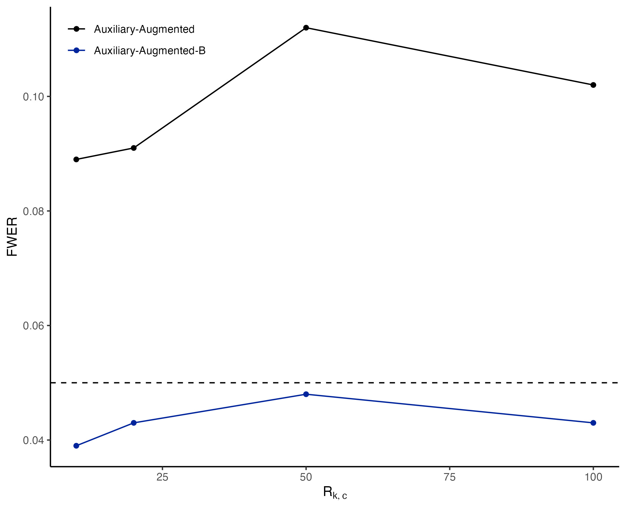
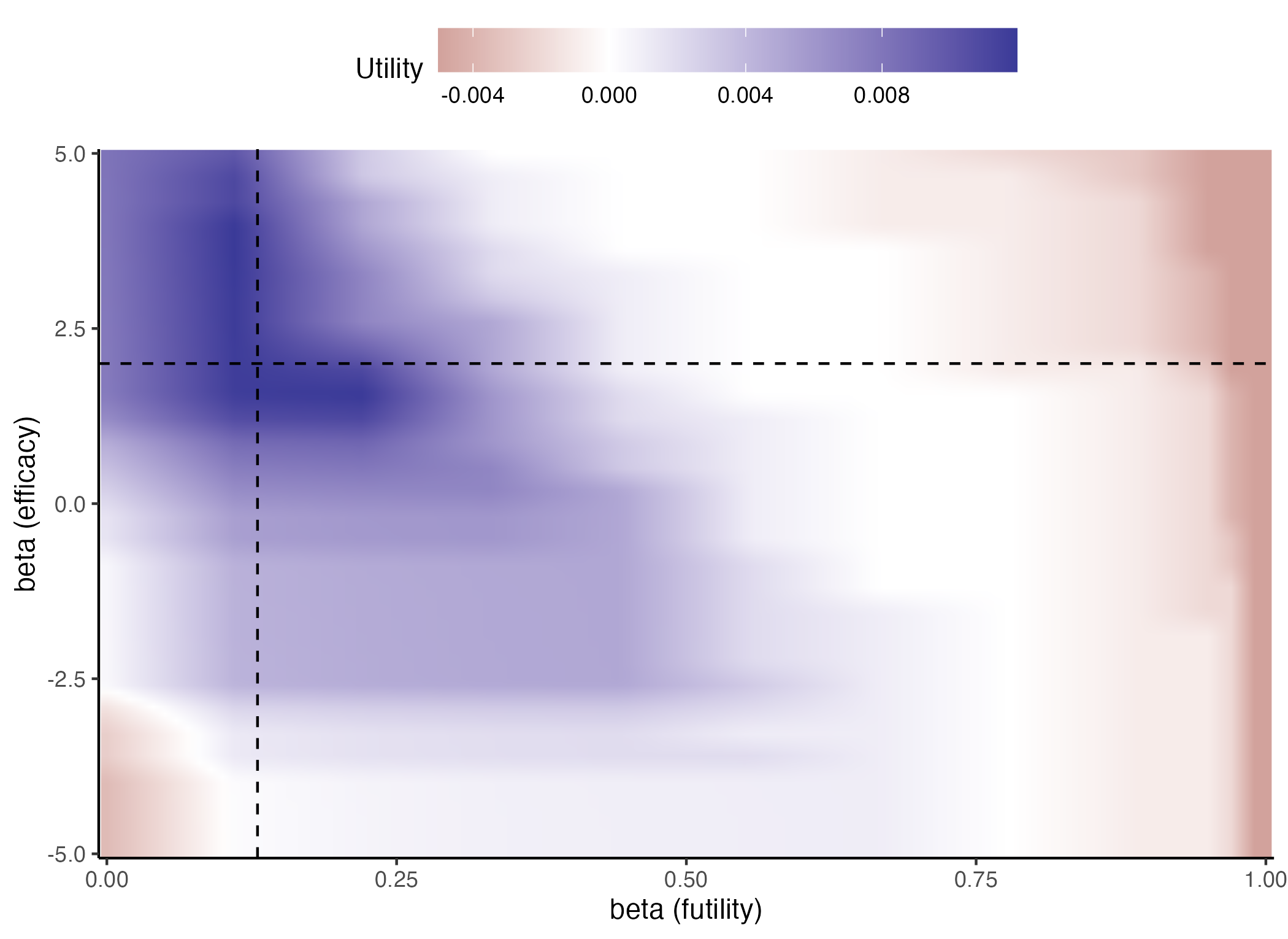
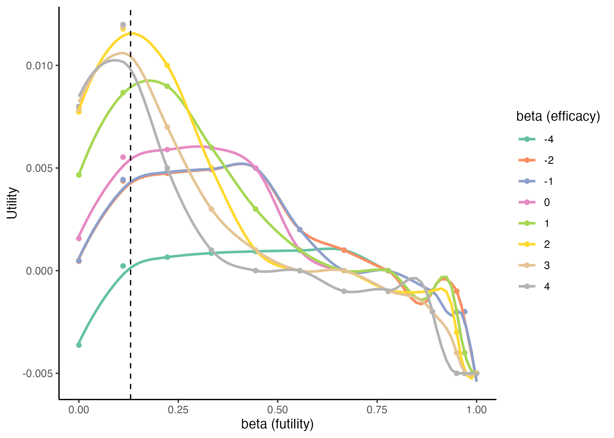
S2 Retrospective analysis with GBM trial data: time-to-event outcomes
We reimplement the retrospective analysis of the CENTRIC trial (Stupp et al.,, 2014) presented in Section 6.1 using time-to-event outcomes. The primary outcome of interest is overall survival (OS), while the auxiliary outcome is progression-free survival (PFS); both are measured from the time of enrollment in the trial. We use the utility function in Equation (9) of the main manuscript and the decision rules described in Section 6.
We rely on a Bayesian prior model for OS and PFS based on the work of Broglio and Berry, (2009), where the OS is decomposed in the sum of PFS and survival post-progression (SPP). In the prior model, if a treatment has a positive effect on OS, this effect is decomposed into the effect on PFS and SPP. We assume that the effect on SPP is a fraction of the effect of PFS. Indicating with the SPP for individual , our prior model can be written as:
Here indicates an exponential distribution with mean Note that in the formulation of Broglio and Berry, (2009) that is to say, all the treatment effects are entirely mediated by PFS. The prior for the treatment effect parameters and follows the same logic as the model introduced in Section 5.1. Alternative models can be used to generate trials with OS and PFS. Examples include the models proposed in Renfro et al., (2011) and Chen et al., (2020)—among others.
Values on the prior parameters used in our example are reported in the caption of Table S5, which also reports relevant characteristics of the trials generated from the prior models.
| Characteristic | Mean (sd) | Min | 1st quantile | Median | 3rd quantile | Max |
|---|---|---|---|---|---|---|
| Median OS (SOC) | 588.4 (389.1) | 70.9 | 337.4 | 489.8 | 717.7 | 4976.3 |
| Median OS (Treated) | 600.3 (447.1) | 42.2 | 337.0 | 487.0 | 726.2 | 7555.1 |
| Median PFS (SOC) | 442.7 (368.0) | 18.3 | 211.3 | 342.3 | 547.1 | 4481.4 |
| Median PFS (Treated) | 457.3 (434.0) | 14.6 | 207.0 | 341.3 | 561.1 | 7125.3 |
| Correlation between PFS and OS | 0.9 (0.1) | 0.0 | 0.9 | 1.0 | 1.0 | 1.0 |
| Proportion of uncersored PFS | 0.8 (0.0) | 0.7 | 0.8 | 0.8 | 0.8 | 0.9 |
| Proportion of uncersored OS | 0.6 (0.0) | 0.5 | 0.6 | 0.6 | 0.7 | 0.8 |
| Time (in days) to collect 50 OS evets | 1101.8 (218.1) | 589.6 | 933.0 | 1074.1 | 1254.8 | 1500.0 |
We added a censoring mechanism to our prior model to generate realistic trials. Censoring times (loss of follow-up) for each trial participant are generated from two independent exponential distributions. Similar to the actual trial, in each trial simulation, the proportion of observed PFS events is approximately , and the proportion of observed OS events is approximately . We assumed an accrual rate of four patients per month. In our experience, this is a realistic accrual rate for nGBM trials. The code to generate the trials from the prior model is available at https://github.com/rMassimiliano/primary_and_auxiliary via the function generate_data_from_prior_survival(). For efficacy decisions, we used the log-rank test as in the original trial (Stupp et al.,, 2014). Other tests, such as the weighted log-rank test, could be used. We perform one interim analysis (IA) after survival events have been collected. All the data available at the time of the IA, such as time to progression for patients still alive, are used for decision-making.
The optimizations to identify the parameters of the design is summarized in Figure S6. The optimum is at
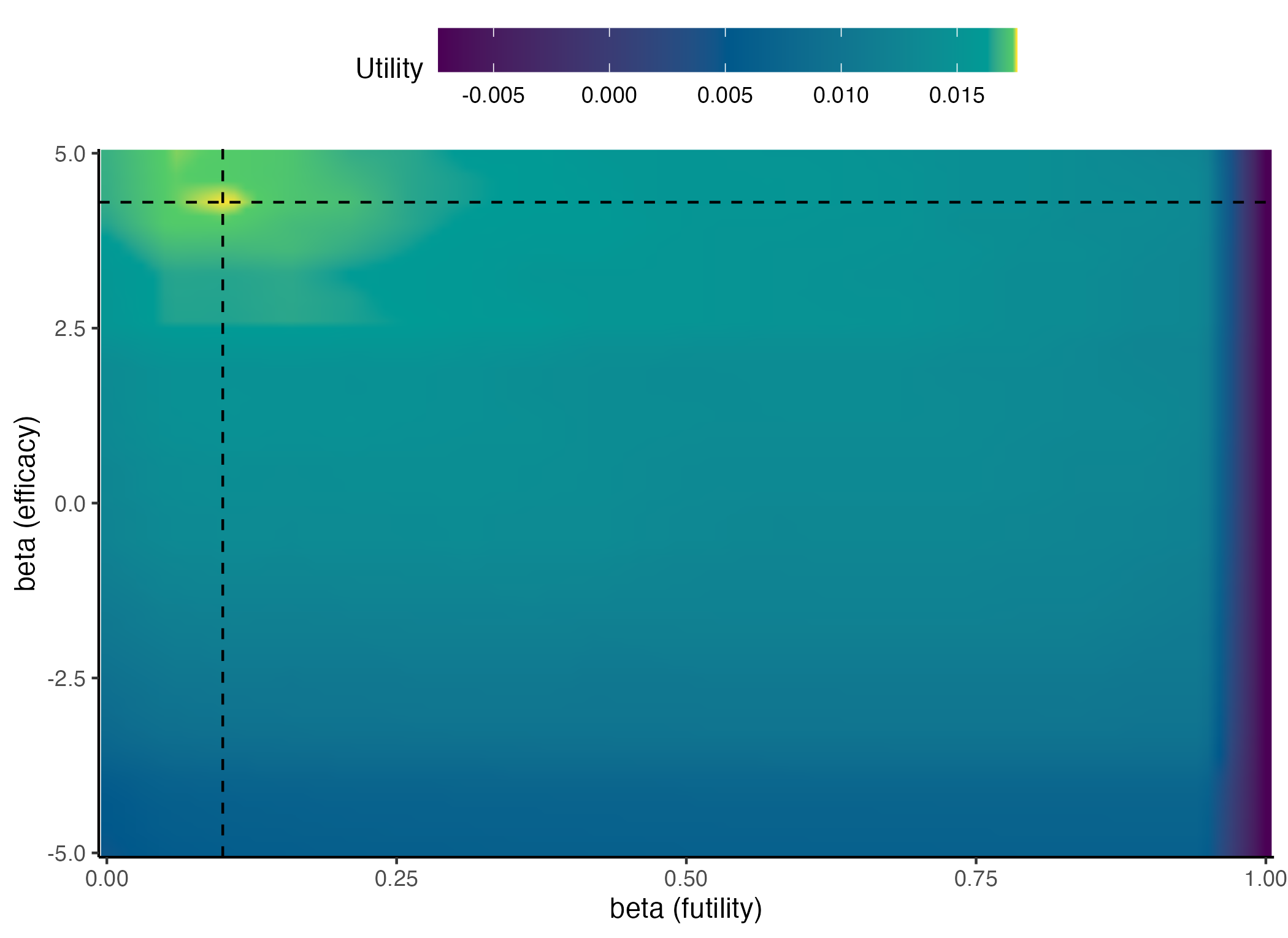
Similarly to Section 6.1, to generate in silico trial replicates tailored to nGBM, we follow these two steps:
-
1.
We sample with replacement a patient from the TMZ+RT group of the CENTRIC dataset. The patient is randomly assigned to either the TMZ+RT or the experimental arm of our in silico trial.
-
2.
If the patient is assigned to our in silico TMZ+RT, we include the actual OS and PFS as primary and auxiliary outcomes. If the patient is assigned to the in silico experimental arm, we use a perturbation of the actual OS and PFS to produce scenarios with positive or negative treatment effects. Specifically, after sampling from the control of CENTRIC, we multiply the observed patient’s OS and PFS by and respectively. The parameters and create in silico trials with treatment effects.
By adjusting the values of and , we created scenarios to examine the trial design, with or without concordance of the treatment effects on primary and auxiliary outcomes. We considered three scenarios: 1. (null scenario) there are no treatment effects on both primary and auxiliary outcome; 2. (concordant effects) and ; 3. (discordant effects) and mimicking a trial where an effect is present for PFS but not on OS, as for lomustine and bevacizumab (Wick et al.,, 2017).
We compare our approach (Auxiliary-Augmented in Table S6) with two alternative trial designs. The first, the Primary-Only design, uses only the primary outcome data for efficacy and futility analyses. This design uses the same group-sequential efficacy rule as the Auxiliary-Augmented design, which is based on a -spending (10) with The futility decisions are based on a Bayesian model that ignores auxiliary information. Specifically, we assume that the OS is exponentially distributed, with mean We let , and , with All the remaining parameters of the design are the same of the Auxiliary-Augmented, including the futility threshold . The other design in our comparisons is the Auxiliary-Only design. It is nearly identical to the Primary-Only design but replaces the primary outcomes with the auxiliary outcomes for the decisions of efficacy and futility.
| Scenario 1 | Scenario 2 | Scenario 3 | ||||
|---|---|---|---|---|---|---|
| null scenario | concordant effects | discordant effects | ||||
| Method | Power | Stop for futility | Power | Stop for futility | Power | Stop for futility |
| Auxiliary-Augmented | 0.04 (0.03; 0.00) | 0.87 | 0.83 (0.78; 0.05) | 0.05 | 0.05 (0.04; 0.01) | 0.70 |
| Primary-Only | 0.05 (0.04; 0.01) | 0.72 | 0.81 (0.76; 0.05) | 0.14 | 0.05 (0.04; 0.01) | 0.72 |
| Auxiliary-Only | 0.05 (0.04; 0.01) | 0.63 | 0.88 (0.60; 0.27) | 0.03 | 0.72 (0.41; 0.31) | 0.06 |
In scenario 1, without treatment effects, all three designs control the type-I error at the The Auxiliary-Augmented design has the largest proportion of trials stopped for futility, compared to for the Primary-Only design, and for the Auxiliary-Only design. In scenario 2, with treatment effects both on primary and auxiliary outcomes, the Auxiliary-Augmented and Primary-Only designs have and power respectively compared to and for the Auxiliary-Only design. The Auxiliary-Augmented design has a smaller percentage of stopping for futility (5%) than the Primary-Only design (14%). This reflects that joint modeling of primary and auxiliary outcomes can effectively capture the presence of treatment effect, reducing the likelihood that a trial is erroneously stopped for futility.
In scenario 3, with a treatment effect only on the auxiliary outcomes, as expected, the Auxiliary-Only design has an inflated type-I error , while the Auxiliary-Augmented and Auxiliary-Only designs control the type-I error at Due to promising auxiliary data, the Auxiliary-Augmented design has an slightly higher sample size of patients compared to of the Auxiliary-Only design. Importantly, in this scenario, the Auxiliary-Augmented prevents inflation of type-I error based on promising auxiliary data.
References
- Arfè et al., (2020) Arfè, A., Alexander, B., and Trippa, L. (2020). Optimality of testing procedures for survival data in the nonproportional hazards setting. Biometrics, 1(12).
- Azzolina et al., (2021) Azzolina, D., Berchialla, P., Gregori, D., and Baldi, I. (2021). Prior elicitation for use in clinical trial design and analysis: A literature review. International Journal of Environmental Research and Public Health, 18(4).
- Belin et al., (2020) Belin, L., Tan, A., De Rycke, Y., and Dechartres, A. (2020). Progression-free survival as a surrogate for overall survival in oncology trials: a methodological systematic review. British Journal of Cancer, 122(11):1707–1714.
- Bélisle, (1992) Bélisle, C. J. (1992). Convergence theorems for a class of simulated annealing algorithms on Rd. Journal of Applied Probability, 29(4):885–895.
- Berger, (1985) Berger, J. O. (1985). Statistical Decision Theory and Bayesian Analysis. Springer Science & Business Media.
- Berry and Eick, (1995) Berry, D. A. and Eick, S. G. (1995). Adaptive assignment versus balanced randomization in clinical trials: a decision analysis. Statistics in medicine, 14(3):231–246.
- Berry et al., (2010) Berry, S. M., Carlin, B. P., Lee, J. J., and Muller, P. (2010). Bayesian adaptive methods for clinical trials. CRC press.
- Betensky, (1997) Betensky, R. A. (1997). Conditional power calculations for early acceptance of h0 embedded in sequential tests. Statistics in Medicine, 16(4):465–477.
- Broglio and Berry, (2009) Broglio, K. R. and Berry, D. A. (2009). Detecting an overall survival benefit that is derived from progression-free survival. JNCI: Journal of the National Cancer Institute, 101(23):1642–1649.
- Burzykowski et al., (2008) Burzykowski, T., Buyse, M., Piccart-Gebhart, M. J., Sledge, G., Carmichael, J., Lück, H.-J., Mackey, J. R., Nabholtz, J.-M., Paridaens, R., Biganzoli, L., Jassem, J., Bontenbal, M., Bonneterre, J., Chan, S., Basaran, G. A., and Therasse, P. (2008). Evaluation of tumor response, disease control, progression-free survival, and time to progression as potential surrogate end points in metastatic breast cancer. Journal of Clinical Oncology, 26(12):1987–1992. PMID: 18421050.
- Buyse and Molenberghs, (1998) Buyse, M. and Molenberghs, G. (1998). Criteria for the validation of surrogate endpoints in randomized experiments. Biometrics, pages 1014–1029.
- Buyse et al., (2000) Buyse, M., Molenberghs, G., Burzykowski, T., Renard, D., and Geys, H. (2000). The validation of surrogate endpoints in meta-analyses of randomized experiments . Biostatistics, 1(1):49–67.
- Chen et al., (2019) Chen, E. Y., Joshi, S. K., Tran, A., and Prasad, V. (2019). Estimation of study time reduction using surrogate end points rather than overall survival in oncology clinical trials. JAMA internal medicine, 179(5):642–647.
- Chen et al., (2020) Chen, X., Hartford, A., and Zhao, J. (2020). A model-based approach for simulating adaptive clinical studies with surrogate endpoints used for interim decision-making. Contemporary Clinical Trials Communications, 18:100562.
- Chugh et al., (2009) Chugh, R., Wathen, J. K., Maki, R. G., Benjamin, R. S., Patel, S. R., Meyers, P. A., Priebat, D. A., Reinke, D. K., Thomas, D. G., Keohan, M. L., et al. (2009). Phase II multicenter trial of imatinib in 10 histologic subtypes of sarcoma using a bayesian hierarchical statistical model. J Clin Oncol, 27(19):3148–53.
- Ciani et al., (2023) Ciani, O., Manyara, A. M., Davies, P., Stewart, D., Weir, C. J., Young, A. E., Blazeby, J., Butcher, N. J., Bujkiewicz, S., Chan, A.-W., et al. (2023). A framework for the definition and interpretation of the use of surrogate endpoints in interventional trials. EClinicalMedicine, 65.
- Delgado and Guddati, (2021) Delgado, A. and Guddati, A. K. (2021). Clinical endpoints in oncology - a primer. Am J Cancer Res, 11(4):1121–1131.
- Demets and Lan, (1994) Demets, D. L. and Lan, K. K. G. (1994). Interim analysis: The alpha spending function approach. Statistics in Medicine, 13(13-14):1341–1352.
- Dickhaus, (2014) Dickhaus, T. (2014). Simultaneous Statistical Inference: With Applications in the Life Sciences. Springer Science & Business Media.
- Dmitrienko et al., (2010) Dmitrienko, A., Tamhane, A., and F., B. (2010). Multiple Testing Problems in Pharmaceutical Statistics. Taylor & Francis: Boca Raton, Florida, Biostatistics Series.
- Dobriban et al., (2015) Dobriban, E., Fortney, K., Kim, S. K., and Owen, A. B. (2015). Optimal multiple testing under a Gaussian prior on the effect sizes. Biometrika, 102(4):753–766.
- Ellenberg and Hamilton, (1989) Ellenberg, S. S. and Hamilton, J. M. (1989). Surrogate endpoints in clinical trials: Cancer. Statistics in Medicine, 8(4):405–413.
- Elliott et al., (2014) Elliott, M. R., Conlon, A. S., Li, Y., Kaciroti, N., and Taylor, J. M. (2014). Surrogacy marker paradox measures in meta-analytic settings. Biostatistics, 16(2):400–412.
- Ensign et al., (1994) Ensign, L. G., Gehan, E. A., Kamen, D. S., and Thall, P. F. (1994). An optimal three-stage design for phase ii clinical trials. Statistics in Medicine, 13(17):1727–1736.
- Finos and Salmaso, (2007) Finos, L. and Salmaso, L. (2007). Fdr-and fwe-controlling methods using data-driven weights. Journal of Statistical Planning and Inference, 137(12):3859–3870.
- Genovese et al., (2006) Genovese, C. R., Roeder, K., and Wasserman, L. (2006). False discovery control with p-value weighting. Biometrika, 93(3):509–524.
- Gordon Lan and Demets, (1983) Gordon Lan, K. K. and Demets, D. L. (1983). Discrete sequential boundaries for clinical trials. Biometrika, 70(3):659–663.
- Guo and He, (2021) Guo, X. and He, X. (2021). Inference on selected subgroups in clinical trials. Journal of the American Statistical Association, 116(535):1498–1506.
- Hoff, (2021) Hoff, P. (2021). Smaller p-values via indirect information. Journal of the American Statistical Association, 0(0):1–16.
- Holm, (1979) Holm, S. (1979). A simple sequentially rejective multiple test procedure. Scandinavian Journal of Statistics, 6(2):65–70.
- Hwang et al., (1990) Hwang, I. K., Shih, W. J., and De Cani, J. S. (1990). Group sequential designs using a family of type I error probability spending functions. Statistics in Medicine, 9(12):1439–1445.
- Jennison and Turnbull, (1999) Jennison, C. and Turnbull, B. W. (1999). Group sequential methods with applications to clinical trials. CRC Press.
- Kemp and Prasad, (2017) Kemp, R. and Prasad, V. (2017). Surrogate endpoints in oncology: when are they acceptable for regulatory and clinical decisions, and are they currently overused? BMC medicine, 15(1):134.
- Kopp-Schneider et al., (2019) Kopp-Schneider, A., Calderazzo, S., and Wiesenfarth, M. (2019). Power gains by using external information in clinical trials are typically not possible when requiring strict type I error control. Biometrical Journal.
- Kropf et al., (2004) Kropf, S., Läuter, J., Eszlinger, M., Krohn, K., and Paschke, R. (2004). Nonparametric multiple test procedures with data-driven order of hypotheses and with weighted hypotheses. Journal of Statistical Planning and Inference, 125(1):31–47. The Third International Conference on Multiple Comparisons.
- Lachin, (2005) Lachin, J. M. (2005). A review of methods for futility stopping based on conditional power. Statistics in Medicine, 24(18):2747–2764.
- Lan et al., (1982) Lan, K. G., Simon, R., and Halperin, M. (1982). Stochastically curtailed tests in long–term clinical trials. Communications in Statistics. Part C: Sequential Analysis, 1(3):207–219.
- Larry Han and Trippa, (2024) Larry Han, A. A. and Trippa, L. (2024). Sensitivity analyses of clinical trial designs: Selecting scenarios and summarizing operating characteristics. The American Statistician, 78(1):76–87. PMID: 38680760.
- LeBlanc et al., (2009) LeBlanc, M., Rankin, C., and Crowley, J. (2009). Multiple histology phase II trials. Clinical Cancer Research, 15(13):4256–4262.
- Lee et al., (2022) Lee, J., Thall, P. F., Lim, B., and Msaouel, P. (2022). Utility-Based Bayesian Personalized Treatment Selection for Advanced Breast Cancer. Journal of the Royal Statistical Society Series C: Applied Statistics, 71(5):1605–1622.
- Lehmann and Romano, (2006) Lehmann, E. L. and Romano, J. P. (2006). Testing statistical hypotheses. Springer Science & Business Media.
- Lewis and Berry, (1994) Lewis, R. J. and Berry, D. A. (1994). Group sequential clinical trials: a classical evaluation of Bayesian decision-theoretic designs. Journal of the American Statistical Association, 89(428):1528–1534.
- Li et al., (2023) Li, X., Yung, G., Lin, J., and Zhu, J. (2023). Estimation of conditional power in the presence of auxiliary data. Statistics in Medicine, 42(24):4319–4332.
- Lindley, (1976) Lindley, D. V. (1976). A Class of Utility Functions. The Annals of Statistics, 4(1):1 – 10.
- Merino et al., (2023) Merino, M., Kasamon, Y., Theoret, M., Pazdur, R., Kluetz, P., and Gormley, N. (2023). Irreconcilable differences: The divorce between response rates, progression-free survival, and overall survival. Journal of Clinical Oncology, 41(15):2706–2712. PMID: 36930853.
- Mushti et al., (2018) Mushti, S. L., Mulkey, F., and Sridhara, R. (2018). Evaluation of overall response rate and progression-free survival as potential surrogate endpoints for overall survival in immunotherapy trials. Clinical Cancer Research, 24(10):2268–2275.
- O’Brien and Fleming, (1979) O’Brien, P. C. and Fleming, T. R. (1979). A multiple testing procedure for clinical trials. Biometrics, pages 549–556.
- Pilz et al., (2012) Pilz, L. R., Manegold, C., and Schmid-Bindert, G. (2012). Statistical considerations and endpoints for clinical lung cancer studies: can progression free survival (pfs) substitute overall survival (OS) as a valid endpoint in clinical trials for advanced non-small-cell lung cancer? Translational Lung Cancer Research, 1(1).
- Pocock, (1977) Pocock, S. J. (1977). Group sequential methods in the design and analysis of clinical trials. Biometrika, 64(2):191–199.
- Prentice, (1989) Prentice, R. L. (1989). Surrogate endpoints in clinical trials: definition and operational criteria. Statistics in medicine, 8(4):431–440.
- Qing et al., (2022) Qing, L., Jianchang, L., Mengya, L., Liwen, W., and Yingying, L. (2022). Using surrogate endpoints in adaptive designs with delayed treatment effect. Statistics in Biopharmaceutical Research, 14(4):661–670.
- Renfro et al., (2011) Renfro, L. A., Carlin, B. P., and Sargent, D. J. (2011). Bayesian Adaptive Trial Design for a Newly Validated Surrogate Endpoint. Biometrics, 68(1):258–267.
- Roeder and Wasserman, (2009) Roeder, K. and Wasserman, L. (2009). Genome-wide significance levels and weighted hypothesis testing. Statistical science, 24(4):398–413.
- Saint-Hilary et al., (2019) Saint-Hilary, G., Barboux, V., Pannaux, M., Gasparini, M., Robert, V., and Mastrantonio, G. (2019). Predictive probability of success using surrogate endpoints. Statistics in Medicine, 38(10):1753–1774.
- Schmidli et al., (2014) Schmidli, H., Gsteiger, S., Roychoudhury, S., O’Hagan, A., Spiegelhalter, D., and Neuenschwander, B. (2014). Robust Meta-Analytic-Predictive Priors in Clinical Trials with Historical Control Information. Biometrics, 70(4):1023–1032.
- Schuster et al., (2004) Schuster, E., Kropf, S., and Roeder, I. (2004). Micro array based gene expression analysis using parametric multivariate tests per gene a generalized application of multiple procedures with data-driven order of hypotheses. Biometrical Journal, 46(6):687–698.
- Simon, (1989) Simon, R. (1989). Optimal two-stage designs for phase ii clinical trials. Controlled Clinical Trials, 10(1):1–10.
- Song et al., (2020) Song, Y., Sun, F., Redline, S., and Wang, R. (2020). Random-effects meta-analysis of combined outcomes based on reconstructions of individual patient data. Research Synthesis Methods, 11(5):594–616.
- Spiegelhalter et al., (1986) Spiegelhalter, D. J., Freedman, L. S., and Blackburn, P. R. (1986). Monitoring clinical trials: Conditional or predictive power? Controlled Clinical Trials, 7(1):8–17.
- Spring et al., (2020) Spring, L. M., Fell, G., Arfe, A., Sharma, C., Greenup, R., Reynolds, K. L., Smith, B. L., Alexander, B., Moy, B., Isakoff, S. J., et al. (2020). Pathologic complete response after neoadjuvant chemotherapy and impact on breast cancer recurrence and survival: a comprehensive meta-analysis. Clinical cancer research, 26(12):2838–2848.
- Stan Development Team, (2023) Stan Development Team (2023). RStan: the R interface to Stan. R package version 2.21.8.
- Stupp et al., (2014) Stupp, R., Hegi, M. E., Gorlia, T., et al. (2014). Cilengitide combined with standard treatment for patients with newly diagnosed glioblastoma with methylated MGMT promoter (CENTRIC EORTC 26071-22072 study): a multicentre, randomised, open-label, phase 3 trial. The Lancet Oncology, 15(10):1100–1108.
- Stupp et al., (2005) Stupp, R., Mason, W. P., van den Bent, M. J., Weller, M., Fisher, B., Taphoorn, M. J., Belanger, K., Brandes, A. A., Marosi, C., Bogdahn, U., Curschmann, J., Janzer, R. C., Ludwin, S. K., Gorlia, T., Allgeier, A., Lacombe, D., Cairncross, J. G., Eisenhauer, E., and Mirimanoff, R. O. (2005). Radiotherapy plus concomitant and adjuvant temozolomide for glioblastoma. New England Journal of Medicine, 352(10):987–996. PMID: 15758009.
- Thall, (2019) Thall, P. F. (2019). Bayesian utility-based designs for subgroup-specific treatment comparison and early-phase dose optimization in oncology clinical trials. JCO Precision Oncology, (3):1–7.
- Tung et al., (2020) Tung, N. M., Robson, M. E., Ventz, S., Santa-Maria, C. A., Nanda, R., Marcom, P. K., Shah, P. D., Ballinger, T. J., Yang, E. S., Vinayak, S., Melisko, M., Brufsky, A., DeMeo, M., Jenkins, C., Domchek, S., D’Andrea, A., Lin, N. U., Hughes, M. E., Carey, L. A., Wagle, N., Wulf, G. M., Krop, I. E., Wolff, A. C., Winer, E. P., and Garber, J. E. (2020). TBCRC 048: Phase II study of olaparib for metastatic breast cancer and mutations in homologous recombination-related genes. Journal of Clinical Oncology, 38(36):4274–4282. PMID: 33119476.
- Vandenberghe et al., (2018) Vandenberghe, S., Duchateau, L., Slaets, L., Bogaerts, J., and Vansteelandt, S. (2018). Surrogate marker analysis in cancer clinical trials through time-to-event mediation techniques. Statistical methods in medical research, 27(11):3367–3385.
- Vanderbeek et al., (2018) Vanderbeek, A. M., Rahman, R., Fell, G., Ventz, S., Chen, T., Redd, R., Parmigiani, G., Cloughesy, T. F., Wen, P. Y., Trippa, L., et al. (2018). The clinical trials landscape for glioblastoma: is it adequate to develop new treatments? Neuro-oncology, 20(8):1034–1043.
- Vanderbeek et al., (2019) Vanderbeek, A. M., Ventz, S., Rahman, R., Fell, G., Cloughesy, T. F., Wen, P. Y., Trippa, L., and Alexander, B. M. (2019). To randomize, or not to randomize, that is the question: using data from prior clinical trials to guide future designs. Neuro-oncology, 21(10):1239–1249.
- Ventz et al., (2021) Ventz, S., Comment, L., Louv, B., Rahman, R., Wen, P. Y., Alexander, B. M., and Trippa, L. (2021). The use of external control data for predictions and futility interim analyses in clinical trials. Neuro-Oncology, 24(2):247–256.
- Ventz and Trippa, (2015) Ventz, S. and Trippa, L. (2015). Bayesian designs and the control of frequentist characteristics: A practical solution. Biometrics, 71(1):218–226.
- Wen et al., (2010) Wen, P. Y., Macdonald, D. R., Reardon, D. A., Cloughesy, T. F., Sorensen, A. G., Galanis, E., DeGroot, J., Wick, W., Gilbert, M. R., Lassman, A. B., Tsien, C., Mikkelsen, T., Wong, E. T., Chamberlain, M. C., Stupp, R., Lamborn, K. R., Vogelbaum, M. A., van den Bent, M. J., and Chang, S. M. (2010). Updated response assessment criteria for high-grade gliomas: Response assessment in neuro-oncology working group. Journal of Clinical Oncology, 28(11):1963–1972. PMID: 20231676.
- Wick et al., (2017) Wick, W., Gorlia, T., Bendszus, M., Taphoorn, M., Sahm, F., Harting, I., Brandes, A. A., Taal, W., Domont, J., Idbaih, A., Campone, M., Clement, P. M., Stupp, R., Fabbro, M., Le Rhun, E., Dubois, F., Weller, M., von Deimling, A., Golfinopoulos, V., Bromberg, J. C., Platten, M., Klein, M., and van den Bent, M. J. (2017). Lomustine and Bevacizumab in progressive glioblastoma. New England Journal of Medicine, 377(20):1954–1963. PMID: 29141164.
- Xie et al., (2019) Xie, W., Halabi, S., Tierney, J. F., Sydes, M. R., Collette, L., Dignam, J. J., Buyse, M., Sweeney, C. J., and Regan, M. M. (2019). A Systematic Review and Recommendation for Reporting of Surrogate Endpoint Evaluation Using Meta-analyses. JNCI Cancer Spectrum, 3(1). pkz002.