FIXED POINTS OF DEEP NEURAL NETWORKS: EMERGENCE, STABILITY, AND APPLICATIONS

Abstract

We present numerical and analytical results on the formation and stability of a family of fixed points of deep neural networks (DNNs). Such fixed points appear in a class of DNNs when dimensions of input and output vectors are the same. We demonstrate examples of applications of such networks in supervised, semi-supervised and unsupervised learning such as encoding/decoding of images, restoration of damaged images among others.

We present several numerical and analytical results. First, we show that for untrained DNN’s with weights and biases initialized by normally distributed random variables the only one fixed point exists. This result holds for DNN with any depth (number of layers) $L$, any layer width $N$, and sigmoid-type activation functions. Second, it has been shown that for a DNN whose parameters (weights and biases) are initialized by “light-tailed” distribution of weights (e.g. normal distribution), after training the distribution of these parameters become “heavy-tailed”. This motivates our study of DNNs with “heavy-tailed” initialization. For such DNNs we show numerically that training leads to emergence of $Q(N,L)$ fixed points, where $Q(N,L)$ is a positive integer which depends on the number of layers $L$ and layer width $N$. We further observe numerically that for fixed $N=N_{0}$ the function $Q(N_{0},L)$ is non-monotone, that is it initially grows as $L$ increases and then decreases to 1.

This non-monotone behavior of $Q(N_{0},L)$ is also obtained by analytical derivation of equation for Empirical Spectral Distribution (ESD) of input-output Jacobian followed by numerical solution of this equation.

Keywords: Deep Neural Network, Fixed Point, Basin of Attraction, Input-Output Jacobian.

I Introduction

In recent years, a variety of new technologies based on Deep Neural Networks (DNNs) also known as Artificial Neural networks (ANNs) have been developed. AI-based technologies have been successfully used in physics, medicine, business and everyday life (see e.g., Yan-Yang ). The two keys theoretical directions in DNN’s theory are the development of novel (i) types of DNNs and (ii) training algorithms.

One of the most important applications of DNN’s is the processing of visual (image or video) information Kaji-Kida ; Hong-Chen . Image transformation (also known as image-to-image translation) means a transform of the original image into another image according to the goals, for instance, stretching the picture without scarifying the image quality. In this example the dimensions of input and output vectors are of the same order of magnitude or just the same. Such DNNs are also called self-mapping transformations and fixed points (FP) play an important role in their studies. For example, in digital image restorationMo-Wa-Zh:22 , the presence of FP means that the corresponding image is free of defects and does not require processing. The closeness of DNN’s output vector to a FP can be used as a stopping criterion for DNNs’ training.

Furthermore, we consider the problem of stability of FP and the formation of basins of attractionShena . Belonging of the input vector to a basins of attraction can be interpreted as belonging of the corresponding image to a certain class of images (e.g., classes may be dogs breeds, if we consider dog images).

Note, that the area of FP applications in DNNs is much wider than image-to-image transformations. For example, FPs play an important role in studying the properties of Hopfield networkHopfield:1982 ; Hopfield:1984 proposed by Nobel Prize winner John Hopfield. This model is widely used in different branches of science from life science, where FPs are responsible for memory formationKrotov-Hopfield:2021 , up to quantum physics, where FPs may be important in the study of phase transitionsKimura-Kate:2024 .

In this work, using numerical and analytical methods, we study the influence of DNN architecture (widths of the layers, DNN’s depth, and activation function), as well as probabilistic distributions of weight matrices on the existence of FPs, their number and their basins of attractions.

II Image-to-Image transformations and Fixed Points of DNN.

A DNN can be written in terms of a sequence of non-linear vector-to-vector transformations. Let $\boldsymbol{x}^{l}$ be an output vector of the $l$-th layer of the DNN.

$$\boldsymbol{x}^{l}=\{x_{j_{l}}^{l}\}_{j_{l}=1}^{n_{l}}\in\mathbb{R}^{n_{l}},\quad l=0,1,\ldots,L\,.$$ (1)

Here $L$ is the DNN’s depth, $\boldsymbol{x}^{0}$/$\boldsymbol{x}^{L}$ is a DNN input/output vector. Layer-to-layer transformation has the form:

$$\boldsymbol{x}^{l+1}=\boldsymbol{\Phi}^{l}(\boldsymbol{x}^{l})=\varphi({\bf W}^{l}\boldsymbol{x}^{l}+{\bf b}^{l}),$$

where

$${\bf W}^{l}=\{W_{j_{l+1},j_{l}}^{l}\}_{j_{l+1},j_{l}=1}^{n_{l+1},n_{l}},\;l=0,...,L-1$$ (2)

are real-valued $n_{l+1}\times n_{l}$ rectangular weight matrices,

$${\bf b}^{l}=\{b_{j_{l}}^{l}\}_{j_{l}=1}^{n_{l}},\;l=0,1,...,L-1$$ (3)

are $n_{l}$-component bias vectors. The function $\varphi\colon\mathbb{R}\rightarrow\mathbb{R}$ is the component-wise activation function — nonlinearity Sigmoid .

Thus, input vector $\boldsymbol{x}^{0}$ to output vector $\boldsymbol{x}^{L}$ transformation provided by DNN is defined as the following function:

$$\boldsymbol{\Phi}(\boldsymbol{x}^{0})=\boldsymbol{\Phi}^{L-1}\circ\boldsymbol{\Phi}^{L-2}\circ\cdots\circ\boldsymbol{\Phi}^{1}\circ\boldsymbol{\Phi}^{0}(\boldsymbol{x}^{0})=\boldsymbol{x}^{L}.$$ (4)

Note, that actually function $\boldsymbol{\Phi}$ depends on input vector $\boldsymbol{x}^{0}$ and also on weights and biases, i.e. $\boldsymbol{\Phi}(\boldsymbol{x})=\boldsymbol{\Phi}(\boldsymbol{x},\alpha)$, where $\alpha$ is a set of all weights and biases. Everywhere below we omit the dependence on $\alpha$ for brevity.

One of the most impressive features of artificial intelligence structures (DNNs, in particular) is a wide area of their applications. The same structures of matrices and vectors can be applied in different branches of sciences, industry and art. The only difference is in the weights and biases. All these values are formed as a result of training — one of the most important ingredient of deep learning. On the other hand, a lot of the modern investigations are devoted to to the study of properties of DNNs at initialization with random weights and biases, see, e.g. penn_uni ; Ba-Co:20 ; Ca-Sc:20 ; Gi-Co:16 ; Li-Qi:00 ; Ma-Co:16 ; Ya:20 . One of the reasons of such interest is that the random initialization of DNN parameters increases the speed and enhances quality of training significantly. In context of such an approach we will assume that the weights and the biases are independent and identically distributed (i.i.d.) random variables.

For DNN solving a classification problem the input vector $\boldsymbol{x}^{0}$ represents an object (e.g. image of a digit, image of a letter, etc.) and the output vector $\boldsymbol{x}^{L}$ represents probabilities of the input $\boldsymbol{x}^{0}$ belonging to each class. If objects are images of symbols, then classes may be the sets containing all images of one digit or letter, etc. Usually, the number of classes $K$ is known apriori e.g., for digits classification problem $K=10$ and for classification of letters of some alphabet $K$ is the number of letters in this alphabet. For such classification problems the size of input vector equals the number of pixels of an image and is much greater than number of classes, i.e. the size of output vector: $n_{0}\gg n_{L}$. At the same time there are several important problems, for which $n_{0}$ and $n_{L}$ are of same order of magnitude or even coincide. For example:

1. Image to Image transformations, where DNNs are used for old photo restoration, for removing films defects (e.g., in old movies), for various visual effects, etc Kaji-Kida ; Hong-Chen . In this case, the result of DNN training is the ability of the network to restore damaged areas of photographs, remove noise, etc. In the particular case of $n_{0}=n_{L}$, fixed points (FP) $\boldsymbol{x}^{*}$, defined by

   $$\boldsymbol{\Phi}(\boldsymbol{x}^{*})=\boldsymbol{x}^{*},$$

   play an important role in determining when an image is free of defects. Fulfillment of this condition means that a picture(s), which is (are) free of defects, $\boldsymbol{x}^{*}$, should turn into itself during image processing using a DNN. This is so called image self-mapping.

2. Image encoding/decodingWand-Cao (for example, verifying IDs of employees using Face ID technologyFaceID ). In this case input vectors $\boldsymbol{x}^{0}\in\mathbb{R}^{n_{0}}$ (integer $n_{0}$ is the size of $\boldsymbol{x}^{0}$) are the photos of employees, obtained from cameras in a building — input pictures. For secure picture transmission to a remote server, in order to provide access control and stop potential, one can use the following DNN-based approach. The example of image encoding/decoding is presented in Fig. 1.

   

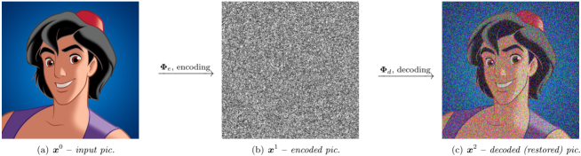
   Figure 1: Schematic illustration of image encoding/decoding using DNN.

   1. For picture encoding, a DNN $\boldsymbol{\Phi}_{c}$: $\mathbb{R}^{n_{0}}\rightarrow\mathbb{R}^{n_{1}}$ is used:

      $$\boldsymbol{\Phi}_{c}(\boldsymbol{x}^{0})=\boldsymbol{x}^{1},$$

      Here $\boldsymbol{x}^{1}\in\mathbb{R}^{n_{1}}$ is encoded picture (integer $n_{1}$ is the size of $\boldsymbol{x}^{1}$, generally, $n_{0}\neq n_{1}$).

   2. For pictures decoding one use the other DNN $\boldsymbol{\Phi}_{d}:\mathbb{R}^{n_{1}}\rightarrow\mathbb{R}^{n_{0}}$. Then $\boldsymbol{\Phi}_{d}(\boldsymbol{x}^{1})=\boldsymbol{x}^{2}$, where $\boldsymbol{x}^{2}\in\mathbb{R}^{n_{0}}$ are the decoded (restored) pictures.

   The goal of the training process for DNN

   $$\boldsymbol{\Phi}(\boldsymbol{x}^{0})=(\boldsymbol{\Phi}_{d}\circ\boldsymbol{\Phi}_{c})(\boldsymbol{x}^{0})=\boldsymbol{x}^{2}$$

   is to obtain $\boldsymbol{x}^{2}=\boldsymbol{x}^{0}$, i.e.,

   $$\boldsymbol{\Phi}(\boldsymbol{x}^{0})=\boldsymbol{x}^{0}.$$

   For simplicity, consider first the case of one employee (i.e. the number of employees $K=1$). To perform training we start with input vectors $\boldsymbol{x}_{T_{1}}\in T_{1}$, where $T_{1}$ is training set containing the first employee’s photos. We then minimize the MSE loss

   $$L_{1}(\alpha)=\sum_{\boldsymbol{x}\in T_{1}}l_{T_{1}}(\boldsymbol{x},\alpha),$$

   where

   $$l_{T_{1}}(\boldsymbol{x},\alpha)=\left\|\boldsymbol{\Phi}(\boldsymbol{x},\alpha)-\boldsymbol{x}^{*}\right\|^{2}.$$ (5)

   Here $\boldsymbol{x}^{*}\in T_{1}$ is “standard” photo of employee stored on access control server. Ultimately we have: $\boldsymbol{\Phi}(\boldsymbol{x}^{*})=\boldsymbol{x}^{*}$, i.e., vector $\boldsymbol{x}^{*}$ is a fixed point of DNN mapping $\boldsymbol{\Phi}$ Piotrowski . If number of employees $K>1$ then the loss function is:

   $$L(\alpha)=\sum_{k=1}^{K}\sum_{\boldsymbol{x}\in T_{k}}l_{T_{k}}(\boldsymbol{x},\alpha),\quad l_{T_{k}}(\boldsymbol{x},\alpha)=\left\|\boldsymbol{\Phi}(\boldsymbol{x},\alpha)-\boldsymbol{x}^{*}_{T_{k}}\right\|^{2},$$

   and $\boldsymbol{x}^{*}_{T_{1}},\boldsymbol{x}^{*}_{T_{2}},\ldots,\boldsymbol{x}^{*}_{T_{K}}$ are the fixed points of $\boldsymbol{\Phi}$. The choice of loss function in this example is quite arbitrary. Instead of MSE (5) one can use, for example, cross-entropy loss functionBuduma ; Sigmoid .

   There are several remarks:

   • The advantage of such method is absence of explicit expressions for data encoding and decoding. This significantly reduces the complicates hacking of encoding/decoding.

   • The natural disadvantage is impossibility to provide exact (bit-to-bit) data recovery, but it is not required in the case of picture encoding/decoding.

   • Another important problem of such approach is stability of encoding/decoding with respect to small fluctuations of input vector (input picture). Such fluctuations are caused by a number of external factors, such as lighting, distance from camera, etc.

   • In particular, this example demonstrates that for DNNs where input and output vector have the same dimensions the number of employees $K$ has nothing in common with the dimension of DNN’s output vector (decoded picture).

3. Unsupervised image classification, i.e. the number of classes $K$ is a priori unknown (number of dog breeds if objects are images of dogs, number of painters in a painting collection, etc.) In this setup, we use DNN $\mathbf{\Phi}$ to transform the image to the generalized image of an object being classified, e.g. “generalized dog”, deprived of any breed specific features. Then our DNN $\boldsymbol{\Phi}$ maps $\mathbb{R}^{n}\rightarrow\mathbb{R}^{n}$, where $n$ is a size of an input image. The loss function for training is chosen as

   $$L(\alpha)=\sum\limits_{\boldsymbol{x}\in T}\|\boldsymbol{\Phi}(\boldsymbol{x},\alpha)-\tilde{\boldsymbol{x}}\|^{2}$$ (6)

   where $\boldsymbol{x}$ is an input vector, $\alpha$ is the set of parameters of DNN $\boldsymbol{\Phi}$ (see above), and $\tilde{\boldsymbol{x}}$ is the given target image of a “generalized dog”.

   Empirically, training leads to the formation of classes via a partition of input vectors space $\Omega$ into disjoint sets $\Omega_{k}$, $k=1,2,\ldots,K$ in the following way: for each FP $\boldsymbol{x}_{k}^{*}$ let $\Omega_{k}$ be its basin of attraction. In current example the number of classes $K$ is the number of dogs breeds in $\Omega$. Each $\boldsymbol{x}^{*}_{k}$ can be considered as “ideal” representative of corresponding breed. The rest of $\Omega$, which does not have FP (if such area exists) we will mark as $\Omega_{0}$.

   As in the previous example, the number of classes $K$ has nothing in common with the dimension of the DNN’s output $\boldsymbol{x}^{L}$.

4. Semi-supervised learning for image classification problem. Again, the number of classes $K$ is a priori unknown. However, a training set $T$ is given. The training set $T$ contains only images from $\tilde{K}<K$ classes and for each image $\boldsymbol{x}\in T$ we know the class where the image is from. Proposed solution of the problem:

   1. For each $k=1,\dotsc,\tilde{K}$ randomly select an image $\boldsymbol{\psi}_{k}\in T$ in the class $k$.

   2. Train DNN $\boldsymbol{\Phi}$ with $n_{0}=n_{L}=n$ using the following loss function

      $$L(\alpha)=\sum\limits_{\boldsymbol{x}\in T}\|\boldsymbol{\Phi}(\boldsymbol{x},\alpha)-\boldsymbol{\psi}_{k(\boldsymbol{x})}\|^{2},$$

      where $k(\boldsymbol{x})$ is the correct class corresponding to the image $\boldsymbol{x}$.

   3. To classify images from unknown classes, use FPs and basins of attraction as described in the previous example.

III Heavy-tailed distributions and DNN’s training: what and why.

In this section we explain where ”heavy-tailed” distributions arise in DNNs. Usually, for initialization of DNN’s weights and biases random variables with “light-tailed” (exponential-tailed) distribution are used. The reason is that the DNNs training is based on stochastic gradient descent (SGD) Buduma . Note, there are several modifications of training process aiming at improving DNNs’ performance. For instance, it was shown that Marchenko-PasturMP pruning of singular values of weight matrices enhances DNN’s accuracyYitzhak . The initialization by random variables with “light-tailed” distribution provides optimal initial state for this method. Actually, such initialization minimizes the number of very large and very small gradients of DNN function $\boldsymbol{\Phi}$ with respect to input vector $\boldsymbol{x}$. That is why we start our investigations of FP from untrained DNN with weight matrices entries and bias vectors components initialized by random variables with normal distribution.

Our aim is to investigate how training affects the FPs and their basins of attraction. It is well established numerically that for trained DNNs the ESD of weight matrices acquires “heavy-tailed” form, regardless of initial distribution of $\alpha$. This phenomenon is a so called Heavy-Tailed Self-Regularization Ma-Ma:17 . For large finite-size matrices ESD $\rho(\lambda)$ appears fully (or partially) “heavy-tailed”, but with finite support of $\lambda$. Moreover, recently it was shown that input-output Jacobian (see also Section V) of a trained DNN has also a “heavy-tailed” ESDBe-Sch:24 .

The effect of Heavy-Tailed Self-Regularization is very important because allow us to use all the tools of Random Matrix Theory for studying spectral properties of DNN’s matrices and their combinations. For example, in Pa_Sl was shown that “heavy-tailed” distribution of $\alpha$ leads to similar distribution of singular values of input-output Jacobian justifying Heavy-Tailed Self-Regularization.

Hence, in our investigation of FP we use Heavy-Tailed Self-Regularization for modeling the properties of trained DNNs.

IV Fixed points and their basins of attraction.

As shown above, FPs play an important role for DNNs in Image to Image transformations. We begin the study with numerical calculations. For simplicity of presentation the dimension of input/output vectors $\boldsymbol{x}$ is taken $n=2$. The space of input vectors $\boldsymbol{x}$ was chosen as a square: $\Omega=[-1,1]\times[-1,1]\subset\mathbb{R}^{2}$.

This square was divided using grid with step $\delta$ (in our calculations $\delta=0.05$):

$$\boldsymbol{x}_{j,l}=\left\{\begin{array}[]{l}x=-1+\delta j,j=0,1,\ldots,\lfloor 2/\delta\rfloor\\ y=-1+\delta l,l=0,1,\ldots,\lfloor 2/\delta\rfloor\end{array}\right.$$ (7)

Here $\lfloor\ldots\rfloor$ denotes an integer part.

For each $\boldsymbol{x}_{j,l}$ the iterative process was executed:

$$\boldsymbol{x}^{m+1}=\boldsymbol{\Phi}(\boldsymbol{x}^{m}),m=1,2,3,\ldots,$$ (8)

where $\boldsymbol{x}^{1}=\boldsymbol{x}_{j,l}$. If $\boldsymbol{\Phi}$ provides contracting mapping on some domain $\omega\in\Omega$, so that $\boldsymbol{x}^{1}\in\omega$, then the process (8) has a limit:

$$\lim_{m\to\infty}\boldsymbol{x}^{m+1}=\boldsymbol{\Phi}(\boldsymbol{x}^{m})=\boldsymbol{x}^{*}\in\omega.$$

The existence of the limit was checked numerically via Cauchy criteria:

$$|\boldsymbol{x}^{m+1}-\boldsymbol{x}^{m}|<\varepsilon,m<N_{0}.$$ (9)

In our calculations $\varepsilon=10^{-5}$, and $N_{0}=50$. If the limits exists, then $\boldsymbol{x}^{m}$ is the fixed point $\boldsymbol{x}^{*}$ corresponding to starting grid point $\boldsymbol{x}^{1}=\boldsymbol{x}_{j,l}$ defined in (7). As a result one can form a list of different fixed points:

$$\boldsymbol{x}_{1}^{*},\boldsymbol{x}_{2}^{*},\ldots,\boldsymbol{x}_{Q}^{*},$$

where all initial points $\boldsymbol{x}_{j,l}$ corresponding to $\boldsymbol{x}_{k}^{*}$ form basin of attraction (partition) $\Omega_{k}$.

We start from untrained DNN with depth $L=2$. Matrix entries (2) and bias vector components (3) are initialized by random variables with normal distribution $N(0,\sigma_{l})$, where $\sigma_{l}=(n_{l})^{-1}$, $l=0,1$. Activation function is “HardTanh”. The results are presented in Fig. 2a. As it seen, the only one fixed point $\boldsymbol{x}=0$ exists, i.e. $Q=1$, and the corresponding basin of attraction is whole set $\Omega$. This result can be interpreted as follows: the untrained DNN can not distinguish input images of employees (see e.g., example 2 in section II).

Next, using the approach based on Heavy-Tailed Self-Regularization (see Ma-Ma:17 ; Pa_Sl and Section III) we model trained DNN by untrained DNN with weights and bias initialized by random variables with Cauchy distribution. In our calculations central point $x_{0}=0$ and scale $\gamma_{l}=(n_{l})^{-1}$. The results are presented in Fig. 2b, c, and d. Fig. 2b corresponds to the same architecture as in Fig. 2a ($L=2$, $n_{l}=[2,100]$), but we see two FP, $Q=2$. Fig. 2c corresponds to $L=3$, $n_{l}=[2,100,100]$, $Q=3$. In Fig. 2d we present the results of calculations for $L=5$, $n_{l}=[2,100,\ldots,100]$, $Q=5$. It is important, that further increase in depth $L$ leads to decrease in $Q$ and the result for $L=20$ is the same as for $L=2$ and normal distribution — the only one FP, $Q=1$. Due to the “weak similarity” effect, discovered in Pa_Sl the choice of activation function $\varphi$ does not change the number of FPs.

Note, that the number of FP, $Q$, and the shapes of basins of attraction $\Omega_{k}$ ($k=1,2,\ldots,Q$) depend on realization of random variables, e.g. weights and biases. In this regard, the question of a possible deterministic limit of $Q$ and stabilization of $\Omega_{k}$ in the random matrix theory (RMT) limit of the weight matrices (2) and bias vectors (3) sizes infinite-width limit $n_{l}\to\infty$ appears. However, the following pattern can be traced: the number of partitions $Q$ first grows with DNN depth $L$, but then decreases. The dependence of FP number $Q=Q(N_{0},L)$ on layers number $L$ for DNNs with layers widths $N_{0}=100$ and with weights and biases initialized by random variables with Cauchy distribution is presented schematically in Fig. 3. This non-monotonic behavior of FP number $Q$ is discussed in the next section.

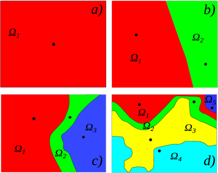
Figure 2: (a) Normal distribution of the matrix elements and bias vector components. Number of layers $L=2$. The same result for Cauchy distribution and $L=20$. (b) Cauchy distribution. $L=2$. (c) Cauchy distribution. $L=3$. (d) Cauchy distribution. $L=5$. The black circles are FPs. Different colors correspond to different basins of attraction $\Omega_{k}$.

Figure 3: Schematic illustration of the dependence of FP number $Q(N_{0},L)$ on layers number $L$ for DNNs with layers widths $N_{0}=100$ and with weights and biases initialized by random variables with Cauchy distribution.

V Input-Output Jacobian

An important tool for studying DNN properties is the input-output Jacobian penn_uni ; Pa_Sl ; Hofman , characterizing the response of DNN output vector to a small perturbation of an input vector. This operator is closely related to the backpropagation operator, mapping output errors to weight matrices, which is the main ingredient of training process. Besides, spectral properties of input-output Jacobian — the ESD — allow one to extract information about DNN training and, hence, to formulate stopping criteria for training.

It occurs, that input-output Jacobian also plays an important role in the study of DNN’s FP (e.g., the conditions for the DNN mapping being a contraction can be determined in terms of this operator). That is why in this paper we perform additional calculations of distribution of input-output Jacobian singular values. Following Pa_Sl , one can write the input-output Jacobian as the following $n_{L}\times n_{0}$ random matrix:

$${\bf J}^{L}=\left\{\frac{\partial\boldsymbol{x}_{j_{L}}^{L}}{\partial\boldsymbol{x}_{j_{0}}^{0}}\right\}_{j_{0},j_{L}=1}^{n_{0},n_{L}}=\prod_{l=0}^{L-1}{\bf D}^{l}{\bf W}^{l},$$ (10)

where diagonal random matrices ${\bf D}^{l}$ are

$${\bf D}^{l}=\{D_{j_{l}}^{l}\delta_{j_{l}k_{l}}\}_{j_{l},k_{l}=1}^{n_{l}},\;D_{j_{l}}^{l}=\left\{\varphi^{\prime}(W^{l}\boldsymbol{x}^{l}+{\bf b}^{l})\right\}_{j_{l}}\;l=0,...,L-1.$$ (11)

Here $\varphi^{\prime}$ means the derivative of activation function $\varphi$.

We will assume, that

$$\mathbf{E}\{{\bf W}^{l}\}=0,\;\mathbf{E}\{({\bf W}^{l})^{2}\}=\sigma^{2}<\infty,\;\mathbf{E}\{({\bf W}^{l})^{4}\}=m_{4}<\infty,$$ (12)

where $\mathbf{E}\{...\}$ denotes a mathematical expectation w.r.t. all random variables.

The functional equation for the resolvent $m_{M^{L}}$ of matrix

$${\bf M}^{L}={\bf J}^{L}({\bf J}^{L})^{T},$$ (13)

was obtained in penn_uni ; Pa_Sl and has the form (see, e.g. (1.24) in Pa_Sl ):

$$m_{M^{L}}(z) =m_{K}(z^{1/L}\Psi_{L}(m_{M^{L}}(z))),$$

$$\Psi_{L}(z) =(1+z)^{1/L}z^{1-1/L}.$$ (14)

Here $m_{M^{L}}(z)$ is the moment generating function:

$$m_{M^{L}}(z)=\sum_{k=1}^{\infty}m_{k}z^{k},\;m_{k}=\int_{0}^{\infty}\lambda^{k}\overline{\nu}_{M^{L}}(d\lambda),$$ (15)

with Normalized Counting Measure (NCM) $\overline{\nu}_{M^{L}}$ (see (1.16)-(1.19) of Pa_Sl ). The relation between $m_{M^{L}}(z)$ and $\overline{\nu}_{M^{L}}$ is

$$m_{M^{L}}(z)=-1-z^{-1}f_{M^{L}}(z^{-1}),$$ (16)

where $f_{M^{L}}$ is the Stieltjes transform of $\overline{\nu}_{M^{L}}$:

$$f_{M^{L}}(z)=\int\frac{\overline{\nu}_{M^{L}}(d\lambda)}{\lambda-z},\quad{\Im}z\neq 0$$

V.1 Numerical solution of functional equation.

In general case the equation (14) can only be solved numerically. The main problem is the existence of multiple roots of (14). To overcome this issue we will use existing asymptotics for $f_{M^{L}}(z)$:

$$f_{M^{L}}(z)\sim-1/z,\quad|z|\gg 1.$$ (17)

For simplicity let us define:

$$w(z)=m_{M^{L}}(1/z)=-1-zf_{M^{L}}(z).$$ (18)

Then (14) acquires the form:

$$w(z) =m_{K}(z^{-1/L}\Psi_{L}(w(z))),$$

$$\Psi_{L}(z) =(1+z)^{1/L}z^{1-1/L}.$$ (19)

Using Banach fixed-point theorem we will find the solution of (19) as the limit of the sequence:

$$w_{n+1}=m_{K}(z^{-1/L}\Psi_{L}(w_{n}))),\quad n=0,1,\ldots$$ (20)

Let us note that $z$ here is a parameter of this iteration scheme and the only variable is $w$. If mapping $m_{K}(w)$ is contracting on some set $\Omega$, then $\forall w_{0}\in\Omega$

$$\lim_{n\to\infty}w_{n}={\bar{w}},$$

and then ${\bar{w}}$ is the root of (19):

$${\bar{w}}=m_{K}(z^{-1/L}\Psi_{L}({\bar{w}})).$$

For numerical solution of (20) the criterion for finding the solution is chosen as

$$|w_{n}-w_{n-1}|<\varepsilon,\ \ n<N_{0},$$ (21)

where $\varepsilon=10^{-5}$ and the maximal number of iterations $N_{0}=50$.

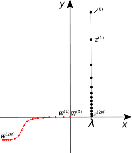
Figure 4: Schematic illustration of calculation algorithm for (20).

As was mentioned above, the equation (14) has, in general, multiple solutions. To chose correct one let us introduce the sequence of complex $z^{(k)}$ as the following:

$$z^{(k)}=\lambda+ib^{N-k},$$ (22)

where $b>1$; $b,\lambda\in\mathbb{R}$ and $N\gg 1,\ N\in\mathbb{Z}$, $k=0,1,2,\ldots,2N$. For $k=0$, $z=z^{(0)}=\lambda+ib^{N}$ is so that $|z|\gg 1$, and according to (18), (17)

$$w_{0}^{(0)}=0.$$

The superscript “$(0)$” means that this initial approximation, i.e. $n=0$ in (20), corresponds to the iteration step with $k=0$. We denote the numerical solution of (20) as ${\bar{w}}^{(0)}$.

Following penn_uni we will decrease $\Im z$, fixing $\Re z=\lambda$, i.e. we will increase $k$ in (22). For $k=1$ the initial approximation $w_{0}^{(1)}$ should be chosen as the numerical solution of (20) obtained for $k=0$ (i.e. $w_{0}^{(1)}={\bar{w}}^{(0)}$). This choice of initial approximation provides asymptotics (17) of $f_{M^{L}}$ at $|z|\gg 1$ and, thus, desired root of (19).

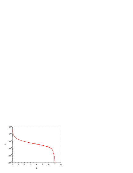
Figure 5: Red line - ESD (in the semi-log scale) of the random matrix ${\bf M}^{L}$ (13) for the Gaussian weights and biases and linear activation function. The network depth $L=2$, layer width $N=10^{3}$ and samples number $10^{3}$. Black line - numerical solution of (19), corresponding to the same network depth $L=2$ and infinite width $N$.

Further, this scheme is repeated for $k=2,3,\ldots,2N$, with $w_{0}^{(k)}={\bar{w}}^{(k-1)}$. As the result we obtain the ${\bar{w}}^{(2N)}$ for $z=z^{(2N)}=\lambda+ib^{-N}\approx\lambda+i0$. The ESD of $M^{L}$ (13) according to the inverse Stieltjes transform has a form

$$\rho(\lambda)\approx\frac{1}{\pi}\Im\left(f_{M^{L}}\right).$$

Substituting $f_{M^{L}}$ from (18)

$$f_{M^{L}}=-\frac{1+{\bar{w}}^{(2N)}}{z^{(2N)}},$$

we finally obtain

$$\rho(\lambda)\approx-\dfrac{1}{\pi}\Im\left(\dfrac{1+{\bar{w}}^{(2N)}}{z^{(2N)}}\right).$$ (23)

Schematic illustration of the proposed algorithm is presented in Fig. 4.

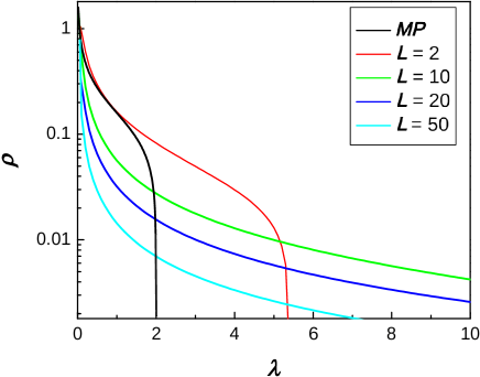
Figure 6: ESD of ${\bf M}^{L}$ (13) corresponding to normal initialization and different number of layers $L$. for $L=1$ activation function $\varphi$ is “Linear” (Marchenko-Pastur distributionMP ). For other values of $L$ activation function $\varphi$ is “HardTanh”.

Let us note that in Pa_Sl the equation (19) was solved in the same way, but with random choice of initial approximation $w_{0}$ in (20). Such initialization does not guarantee the desired root of the equation and the criterion for whether the root is correct is smoothness of $\rho(\lambda)$ in (23). The approach proposed here guarantees the correct choice of root of (19) and does not require any additional verification.

The solution of (14) for linear activation function (24), is presented in Fig. 5 (black curve). Red curve corresponds to the direct numerical calculation of the eigenvalues distribution of the random matrix (13), corresponding to DNN with $L=2$, layer width $N=10^{3}$. The distribution of eigenvalues was obtained by averaging over $10^{3}$ realizations. One can see good agreement between the the results for finite-size system and infinite-size one. The only difference is in the neighborhood of soft-edge of spectra (maximal value of $\lambda$). For finite-size system this edge is random, for infinite-size system – deterministic. On the other hand, the behavior of Jacobian (10) eigenvalues determines the existence of FP and boundaries of partitions (basins of attraction). For example, $\|{\bf J}^{L}\|<1$ is sufficient for the DNN mapping to be a contraction. The obtained result confirms our assumption that in the RMT limit the number of FPs $Q$ and corresponding basins $\Omega_{k}$, $k=1,2,\ldots,Q$ may be non-random.

In Fig. 6, the solutions of (14) corresponding to initialization of weights by random variables with normal distribution and various numbers of layers $L$ are shown. The activation function $\varphi$ is “Linear”. The case of single layer $L=1$ corresponds to Marchenko-Pastur distribution MP . One can notice that, with increase of $L$ the curve is pressed towards the $\lambda$-axis, forming a narrow peak at $\lambda=0$. So, as $L\to\infty$ the ESD $\rho(\lambda)\to\delta(\lambda)$. It means that the eigenvalues of Jacobian (10) tend to zero, providing contraction mapping $\forall\boldsymbol{x}\in\Omega$ and, hence, only one FP $\boldsymbol{x}^{*}$ may exists. This result is also in full agreement with our numerical simulations, demonstrating that the number of FPs $Q\to 1$ as $L\to\infty$.

The equation (14) is not applicable for “heavy-tailed” distributions due to violation of (12), but direct numerical calculation of eigenvalues of (13) shows that ESD takes a $\delta$-like shape as $L\to\infty$ even for “heavy-tailed” distributions. We used Cauchy distribution for calculations and the results are presented in Fig. 7.

Numerical solution of (19) was carried out with the following activation functions: “Linear”, “ReLU”, “Hard Tanh” and “Erf”. The corresponding moment generating functions $m_{M^{L}}$ are penn_uni :

• For “Linear” activation:

  $$m_{M^{L}}(z)=\frac{z}{1-z}$$ (24)

• For “ReLU” activation:

  $$m_{M^{L}}(z)=\frac{1}{2}\frac{z}{1-z}$$

• For “HardTanh” activation:

  $$m_{M^{L}}(z,q)={\rm erf}\left(1/\sqrt{2q}\right)\frac{z}{1-z}$$

• For ”Erf” activation:

  $$m_{M^{L}}(z,q)=\frac{z}{\sqrt{2\pi q}}\Phi\left(z,1/2,\frac{1+\pi q}{\pi q}\right)$$

  where $\Phi$ is a special function known as the Lerch transcendent.

  $$\Phi(z,s,\alpha)=\sum_{n=0}^{\infty}\frac{z^{n}}{(n+\alpha)^{s}}$$

Due to “weak similarity” mentioned above, the results differ quantitatively only and, hence, were not presented here.

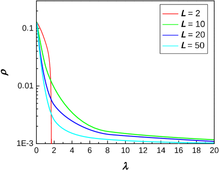
Figure 7: ESD of ${\bf M}^{L}$ (13) corresponding to Cauchy initialization and various numbers of layers $L$. The activation function $\varphi$ is “HardTanh”.

VI Summary of Results and discussion

We studied the existence of fixed points and corresponding basins of attraction of the class of DNNs with the same dimensions of input and output vectors. Such DNNs play an important role in various image-to-image transformations, such as image encoding/decoding, semi-supervised image classification, various visual effects, etc.

We first considered untrained DNNs with random initialization of weight matrices according to “light-tailed” distribution (exponential decay of the tail), e.g., normal distribution. Here we showed the existence of the unique fixed point (FP) for any DNNs layer width $N$, any DNNs depth $L$ and a wide class of “sigmoid”-type activation functions.

Proposition 1

Consider an untrained DNN $\boldsymbol{\Phi}(\boldsymbol{x})$ with random initialization of weight matrices according to “light-tailed” distribution (exponential decay of the tail), e.g., normal distribution. Then there exists a unique fixed point (FP) of $\boldsymbol{\Phi}(\boldsymbol{x})$ for any DNN’s layer width $N$, any DNN’s depth $L$ and a wide class of “sigmoid”-type activation functions.

We next turn our attention to the trained DNNs. Note, that such DNNs typically have “heavy-tailed” distribution (e.g., Cauchy distribution) of weights Ma-Ma:17 ; Pa_Sl . The key result of this paper shows that the change from “light-tailed” to “heavy-tailed” distributions critically affects the number of fixed points and their basins of attractions. Specifically we established the following proposition.

Proposition 2

Let every layer of the trained DNN $\boldsymbol{\Phi}(\boldsymbol{x})$ have the same width $N_{0}$. Then the number of FP $Q(N_{0},L)$ increases with DNN’s depth $L$ up to some value $L_{0}$ and then decreases to $Q(N_{0},L)=1$ as $L\to\infty$. Our numerical calculations indicate stability of these FP. Moreover, each FP of $\boldsymbol{\Phi}(\boldsymbol{x})$ is an interior point of its basin of attraction.

Remarks. (i) In context of example 2 in section II the Proposition 1 means that untrained DNN can not identify employees images correctly whereas trained one can.

(ii) Proposition 2 implies that DNN training leads to formation of extra FPs and corresponding basins of attraction.

The issue of practical importance is to optimize architecture of DNN to obtain the required number of fixed points $Q(N,L)$ which depends on specific application (e.g. the number of employees in the example 2 of section II). In this work we studied the dependence of $Q(N,L)$ on the depths $L$ for fixed $N_{0}$. We showed that it is non-monotone and there exists an optimal DNN’s depths $L_{0}$ for given number of classes (e.g., employees number in example 2 in section II).

Out analytical results are based analysis of spectral properties of input/output Jacobian for DNN’s with random initialization penn_uni ; Pa_Sl ; Be-Sch:24 . These results complement numerical calculations.

VII Acknowledgments

The work of V.S. was supported by NSF Grant “International Multilateral Partnerships for Resilient Education and Science System in Ukraine” (IMPRESS-U): N240122. The work of L.B. was partially supported by the same NSF Grant. The authors are grateful to Ievgenii Afanasiev for many discussions and useful suggestions.

References

- (1) Y. Yan, S. Yang, Y. Wang, J. Zhao, F. Shen, Review Neural Networks about Image Transformation Based on IGC Learning Framework with Annotated Information, arXiv:2206.10155v1 (2022).
- (2) S. Kaji, S. Kida, Overview of image-to-image translation by use of deep neural networks: denoising, super-resolution, modality conversion, and reconstruction in medical imaging, arXiv:1905.08603 (2019).
- (3) W. Hong, T. Chen, M. Lu, S. Pu and Z. Ma, Efficient Neural Image Decoding via Fixed-Point Inference, in IEEE Transactions on Circuits and Systems for Video Technology, 31 (9) 3618-3630, (2021).
- (4) C. Mou, Q. Wang, J. Zhang, Deep Generalized Unfolding Networks for Image Restoration, arXiv:2204.13348 (2022).
- (5) J. Shena, K. Kaloudis, Ch. Merkatas, M. A. F. Sanjuán, On the approximation of basins of attraction using deep neural networks, arXiv:2109.06564v1 (2021).
- (6) J. Hopfield, Neural networks and physical systems with emergent collective computational abilities, Proceedings of the National Academy of Sciences 79(8), 2554 (1982).
- (7) J. Hopfield, Neurons with graded response have collective computational properties like those of two-state neurons., Proceedings of the National Academy of Sciences 81 (10), 3088 (1984).
- (8) D. Krotov, J. Hopfield, Large Associative Memory Problem in Neurobiology and Machine Learning, arXiv:2008.06996 (2021).
- (9) T. Kimura, K. Kato, Analysis of Discrete Modern Hopfield Networks in Open Quantum System, arXiv:2411.02883 (2024).
- (10) L. Berlyand, P.-E. Jabin, Mathematics of Deep Learning: An Introduction, Walter de Gruyter GmbH & Co KG, 132 pages (2023).
- (11) J. Pennington, S. S. Schoenholz, S. Ganguli, The Emergence of Spectral Universality in Deep Networks. arXiv:1802.09979v1 (2018).
- (12) Y. Bahri, J. Kadmon, J. Pennington, S. Schoenholz, J. Sohl-Dickstein, and S. Ganguli, Statistical mechanics of deep learning, Annual Review of Condensed Matter Physics, 11 501–528 (2020).
- (13) C. Gallicchio and S. Scardapane, Deep randomized neural networks, in Recent Trends in Learning From Data. Studies in Computational Intelligence, 896, eds. L. Oneto, N. Navarin, A. Sperduti and D. Anguita (Springer, Heidelberg, 2020).
- (14) R. Giryes, G. Sapiro and A. M. Bronstein, Deep neural networks with random Gaussian weights: A universal classification strategy?. IEEE Trans. Signal Processes 64 3444–3457 (2016).
- (15) Z. Ling, X. He and R. C. Qiu, Spectrum concentration in deep residual learning: a free probability approach, IEEE Acess 7 105212–105223, arxiv:1807.11697 (2019).
- (16) A. G. de G. Matthews, J. Hron, M. Rowland, R. E. Turner,and Z. Ghahramani. Gaussian process behaviour in wide deep neural networks, Int. Conf. on Learn. Represent, arxiv:1804.1127100952 (2018).
- (17) G. Yang, Tensor programs III: neural matrix laws, arxiv:2009.10685v1 (2020).
- (18) J. Wang, R. Cao, N.J. Brandmeir, et al. Face identity coding in the deep neural network and primate brain. Commun Biol 5, 611 (2022).
- (19) J. Wang, R. Cao, N.J. Brandmeir, et al, Face identity coding in the deep neural network and primate brain, Commun Biol 5, 611 (2022).
- (20) T.J. Piotrowski, R.L.G. Cavalcante, M. Gabor, Fixed points of nonnegative neural networks, Journal of Machine Learning Research, 25(139) 1-40, arXiv:2106.16239v9 (2024).
- (21) N. Buduma, Fundamentals of Deep Learning, O’Reilly Media, Inc., 2-nd edition, 387 p, 2017.
- (22) V. Marchenko, L. Pastur, The eigenvalue distribution in some ensembles of random matrices, Math. USSR Sbornik 1, 457–483 (1967).
- (23) L. Berlyand, E. Sandier, Y. Shmalo, and L. Zhang, Enhancing Accuracy in Deep Learning Using Random Matrix Theory, Journal of Machine Learning. 3(4) 347-412, (2024).
- (24) C.H. Martin and M.W. Mahoney, Implicit self-regularization in deep neural networks: evidence from random matrix theory and implications for learning, Journal of Machine Learning Research 22, 1-73 (2021).
- (25) N. Belrose, A. Scherlis, Understanding gradient descent through the training Jacobian, arXiv:2412.07003v2 (2024).
- (26) L. Pastur, V. Slavin, On random matrices arising in deep neural networks: General iid case, Random Matrices: Theory and Applications 12 (01), 2250046 (2023).
- (27) J. Hoffman, D.A. Roberts, Sh. Yaida, Robust Learning with Jacobian Regularization, arXiv:1908.02729v1 (2019).