Collaborative Spacecraft Servicing under Partial Feedback using Lyapunov-based Deep Neural Networks

Abstract

Multi-agent systems are increasingly applied in space missions, including distributed space systems, resilient constellations, and autonomous rendezvous and docking operations. A critical emerging application is collaborative spacecraft servicing, which encompasses on-orbit maintenance, space debris removal, and swarm-based satellite repositioning. These missions involve servicing spacecraft interacting with malfunctioning or defunct spacecraft under challenging conditions, such as limited state information, measurement inaccuracies, and erratic target behaviors. Existing approaches often rely on assumptions of full state knowledge or single-integrator dynamics, which are impractical for real-world applications involving second-order spacecraft dynamics. This work addresses these challenges by developing a distributed state estimation and tracking framework that requires only relative position measurements and operates under partial state information. A novel $\rho$-filter is introduced to reconstruct unknown states using locally available information, and a Lyapunov-based deep neural network adaptive controller is developed that adaptively compensates for uncertainties stemming from unknown spacecraft dynamics. To ensure the collaborative spacecraft regulation problem is well-posed, a trackability condition is defined. A Lyapunov-based stability analysis is provided to ensure exponential convergence of errors in state estimation and spacecraft regulation to a neighborhood of the origin under the trackability condition. The developed method eliminates the need for expensive velocity sensors or extensive pre-training, offering a practical and robust solution for spacecraft servicing in complex, dynamic environments.

1 Introduction

Multi-agent systems play a role in space applications such as distributed space systems, resilient constellations, and autonomous rendezvous and docking operations (e.g., [1, 2, 3]). A rapidly advancing area within this domain is collaborative spacecraft servicing, which includes on-orbit maintenance, space debris removal, and swarm-based satellite repositioning (e.g., [3, 4, 5]). While current multi-agent spacecraft servicing scenarios often involve a small number of agents, typically between 2 to 5 spacecraft (e.g., [6]), future missions are expected to comprise larger constellations of 10 to 20 or more agents, necessitating the development of decentralized control strategies that can efficiently coordinate and adapt to the complexities of these systems (e.g., [7]). The adoption of collaborative and decentralized approaches in these missions offers several benefits, including enhanced reliability, reduced costs, and improved safety, as multiple servicing spacecraft can work together to accomplish complex tasks while minimizing the risk of single-point failures. These missions often involve multiple servicing spacecraft performing tasks such as approaching, inspecting, or rendezvousing with a non-functional or malfunctioning spacecraft that may be in an uncontrolled tumble or exhibiting anomalous behavior.

The space environment introduces unique challenges for these scenarios. These include limited knowledge of the defunct spacecraft, reduced state accuracy due to measurement errors, and partial or unavailable state measurements (e.g., [8, 9]). Such constraints necessitate methods for reconstructing the state of the spacecraft using incomplete information. Furthermore, the characterization of defunct spacecraft in complex servicing scenarios is often complicated by orbital dynamics, poor lighting conditions, unknown physical properties, and erratic behaviors (e.g., [10, 11, 12, 13]). In such cases, state estimation alone may prove inadequate, requiring the additional capability to learn the dynamics of the defunct spacecraft to predict its behavior and devise effective servicing strategies.

Neural networks (NNs) are frequently employed to approximate the unstructured uncertainty inherent in spacecraft dynamics, particularly in scenarios where classical physics-based models may be insufficient or impractical (e.g., [14, 15, 16, 17]). In contrast to white-box approaches, which rely on explicit physical equations, NNs offer a powerful black-box paradigm that can estimate unknown dynamics under challenging space weather conditions, including low Earth orbit, electromagnetic interactions with unknown gravitational fields, uncertain gravitational perturbations and atmospheric drag. The ability of NNs to learn complex patterns and relationships in data makes them well-suited for capturing nonlinearities and uncertainties that arise in spacecraft systems. Furthermore, recent advances in deep neural networks (DNNs) have significantly improved function approximation capabilities, enabling more accurate estimation of uncertain dynamics (e.g., [18]).

To mitigate the uncertainties inherent in complex systems, traditional machine learning approaches typically rely on offline training of NNs using pre-collected datasets. However, this methodology has several limitations: the required datasets can be difficult to obtain, may not accurately reflect the operating conditions of the environment, and fail to adapt online to discrepancies between the pretrained data and actual system behavior. In contrast, adaptive control offers a promising alternative by enabling real-time estimation of unknown model parameters while providing stability guarantees for the system. While shallow NNs have enabled online adaptation for decades, DNNs offer enhanced performance, but often require extensive offline pre-training, which can be challenging in dynamic environments. However, recent breakthroughs in Lyapunov-based DNNs (Lb-DNNs) overcome the challenges associated with nonlinear nested uncertain parameters (e.g., [19, 20, 21, 22, 23]), enabling the construction of analytically-derived update laws based on Lyapunov-based stability analysis, which provide convergence and boundedness guarantees while allowing for real-time adaptation without pre-training requirements. Several results have demonstrated the effectiveness of adaptive NNs in spacecraft rendezvous applications, including estimating nonlinear dynamical models in the presence of $J_{2}$ perturbations and orbit uncertainty estimation (e.g., [14, 15]), and uncertain spacecraft dynamics (e.g., [16, 17]).

The work in [24] pioneered the use of Lb-DNNs for distributed state estimation and tracking in multi-agent systems, while also introducing the notion of trackability. To illustrate trackability, consider a network of fixed cameras observing a dynamic object. Each camera can capture only a subset of the information required to fully determine the object’s state. Independent estimation by each camera results in incomplete information. By enabling the cameras to share their individual estimates, the network forms a collaborative framework that leverages collective information. When generalized to multi-agent systems, this approach leads to the concept of trackability, which quantifies the richness of information required for accurate state estimation in a decentralized system.

For example, in a two-dimensional system with two agents tracking a single target, if each agent measures only one degree of freedom and lacks communication with the other, the agents can only align collinearly with the target. However, successful tracking requires the agents to share partial measurements to achieve complete state reconstruction. This concept is particularly relevant for multi-agent spacecraft servicing, where inter-agent communication can significantly enhance state estimation and servicing capabilities.

While [24] demonstrated exponential state estimation and tracking within a neighborhood of the object of interest, it relied on assumptions that are impractical for spacecraft servicing, such as single-integrator dynamics and full relative state information. Extending these results to second-order spacecraft dynamics while assuming full relative velocity information is unrealistic, as relative velocity sensors are often costly and energy-intensive. Therefore, there is a need for a distributed observer capable of reconstructing relative velocities using only relative position measurements.

This work addresses the challenges of spacecraft servicing by eliminating the restrictive assumptions in [24]. The developed method relies solely on relative position measurements and accommodates partial state information of the defunct spacecraft. A novel $\rho$-filter is developed, extending the work in [25], to reconstruct unknown states using locally available information. Through Lyapunov-based stability analysis, the method guarantees exponential convergence of the defunct spacecraft’s state estimates and regulates the servicing spacecraft to a neighborhood of the defunct satellite’s state, provided the trackability condition is satisfied.

2 Notation and Preliminaries

The study of multi-agent systems involves challenges due to the complexity arising from multiple interacting agents and nonlinear dynamics. To address these challenges effectively, several mathematical tools and notational conventions are introduced in this section. Linear algebra provides a compact and efficient way to represent agent states, interactions, and transformations using vectors and matrices, while eigenvalue analysis supports stability and convergence studies. The networked nature of multi-agent systems is naturally modeled using graphs, and algebraic graph theory offers powerful methods to analyze key properties such as consensus, stability, and connectivity. Finally, deep neural networks play an increasingly important role in adaptive control of multi-agent systems, leveraging their ability to approximate complex mappings and learn from data in uncertain and dynamic environments. These tools and notations form the foundational elements necessary for modeling, analysis, and control in the context of multi-agent systems.

Denote by $\mathbf{1}_{n}\in\mathbb{R}^{n}$ the column vector of length $n>1$ whose entries are all ones. Similarly, $\mathbf{0}_{n}\in\mathbb{R}^{n}$ denotes the column vector of length $n>1$ whose entries are all zeroes. For $m,n>1$, $\mathbf{0}_{m\times n}\in\mathbb{R}^{m\times n}$ denotes the $m\times n$ zero matrix. The $p\times p$ identity matrix and the $p\times 1$ column vector of ones are denoted by $I_{p}$ and $1_{p}$, respectively. Given $M\in\mathbb{Z}_{>0}$, the enumeration operation $[\cdot]$ is defined as $[M]\triangleq\{1,2,...,M\}$. Let $n,m\in\mathbb{Z}_{>0}$ with $m>n$. The Euclidean norm of $r\in\mathbb{R}^{n}$ is $\left\|r\right\|\triangleq\sqrt{r^{\top}r}$. Given a positive integer $N$ and collection $\{x_{i}\}_{i\in[N]}\subset\mathbb{R}^{n}$, let $(x_{i})_{i\in[N]}\triangleq[x_{1}^{\top},x_{2}^{\top},...,x_{N}^{\top}]^{\top}\in\mathbb{R}^{nN}$. Given $H\in\mathbb{R}^{m\times m}$ with columns $\{h_{i}\}_{i\in[n]}\subset\mathbb{R}^{m},\text{vec}(H)=[h_{1}^{\top},h_{2}^{\top},\ldots,h_{n}^{\top}]^{\top}\in\mathbb{R}^{mn}$. The Frobenius norm is denoted by $\left\|\cdot\right\|_{F}\triangleq\left\|\mathrm{vec}(\cdot)\right\|$. The Kronecker product of $A\in\mathbb{R}^{p\times q}$ and $B\in\mathbb{R}^{m\times n}$ is denoted by $A\otimes B\in\mathbb{R}^{pm\times qn}$. Given any $A\in\mathbb{R}^{p\times a}$, $B\in\mathbb{R}^{a\times r}$, and $C\in\mathbb{R}^{r\times s}$, the vectorization operator satisfies the property $\mathrm{vec}(ABC)=(C^{\top}\otimes A)\mathrm{vec}\left(B\right)$. Differentiating on both sides with respect to $\mathrm{vec}\left(B\right)$ yields the property

$$\frac{\partial}{\partial\mathrm{vec}\left(B\right)}\mathrm{vec}(ABC) = (C^{\top}\otimes A).$$ (1)

The maximum and minimum eigenvalues of $G=G^{\top}$ are denoted by $\lambda_{\text{max}}(G)\in\mathbb{R}$ and $\lambda_{\text{min}}(G)\in\mathbb{R}$, respectively. The spectral norm of $A\in\mathbb{R}^{n\times n}$ is defined as $\sigma_{\max}\left(A\right)\triangleq\sqrt{\lambda_{\max}\left(A^{\top}A\right)}$. For $A\in\mathbb{R}^{c\times c}$ and $B\in\mathbb{R}^{d\times d}$, let the block diagonalization operator be defined as $\text{blkdiag}(A,B)=\left[\begin{array}[]{cc}A&\mathbf{0}_{c\times d}\\ \mathbf{0}_{c\times d}&B\end{array}\right]\in\mathbb{R}^{(c+d)\times(c+d)}$. The right-to-left matrix product operator is represented by $\stackrel{{\scriptstyle\curvearrowleft}}{{\prod}}$, i.e., $\stackrel{{\scriptstyle\curvearrowleft}}{{\stackrel{{\scriptstyle[}}{{p}}=1]{m}{\prod}}}A_{p}=A_{m}\ldots A_{2}A_{1}$ and $\stackrel{{\scriptstyle\curvearrowleft}}{{\stackrel{{\scriptstyle[}}{{p}}=a]{m}{\prod}}}A_{p}=I$ if $a>m$.

The space of essentially bounded Lebesgue measurable functions is denoted by $\mathcal{L}_{\infty}$. For $A\subseteq\mathbb{R}^{n}$ and $B\subseteq\mathbb{R}^{m}$, let ${\tt C}(A,B)$ denote the set of continuous functions $f:A\to\mathbb{R}^{m}$ such that $f(A)\subseteq B$. A function with $k$ continuous derivatives is called a $\mathtt{C}^{k}$ function.

2.1 Algebraic Graph Theory

Let $\mathcal{G}\triangleq(\mathcal{V},E)$ represent a static and undirected graph with number of nodes $N\in\mathbb{Z}_{\geq 2}$, where the node set is denoted by $\mathcal{V}\triangleq\left[N\right]$, and the edge set is denoted by $E\subseteq\mathcal{V}\times\mathcal{V}$. An edge between nodes $i$ and $k$ belongs to the edge set $(\text{i.e., }(i,k)\in E)$ if and only if node $i$ can send information to node $k$. Since the graph $\mathcal{G}$ is undirected, $(i,k)\in E$ if and only if $(k,i)\in E$. An undirected graph is connected whenever there exists a sequence of edges in $E$ linking any two distinct nodes. The neighborhood set of node $i$ is $\mathcal{N}_{i}\triangleq\{k\in\mathcal{V}\setminus\{i\}:(k,i)\in E\}$. Let $\mathcal{A}\triangleq\left[a_{ik}\right]\in\mathbb{R}^{N\times N}$ be the adjacency matrix of $\mathcal{G}$, where $a_{ik}=1$ if $(k,i)\in E$ and $a_{ik}=0$ otherwise. Within this work, no self-loops are considered. Therefore, $a_{ii}\triangleq 0$ for all $i\in\mathcal{V}$. The degree matrix of $\mathcal{G}$ is $\mathcal{D}\triangleq\text{diag}(\mathcal{A}\cdot 1_{N})\in\mathbb{R}^{N\times N}$. Using the degree and adjacency matrices, the Laplacian matrix of the graph $\mathcal{G}$ is $\mathcal{L}\triangleq\mathcal{D}-\mathcal{A}$.

2.2 Deep Neural Network Model

Let $\kappa\in\mathbb{R}^{L_{0}}$ denote a DNN input, and $\theta\in\mathbb{R}^{p}$ denote the vector of DNN parameters (i.e., weights and bias terms). A fully-connected feedforward DNN $\Phi(\kappa,\theta)$ with $k\in\mathbb{Z}_{>0}$ hidden layers and output size $L_{k+1}\in\mathbb{Z}_{>0}$ is defined using a recursive relation $\varphi_{j}\in\mathbb{R}^{L_{j+1}}$ modeled as [19]

$$\varphi_{j} \triangleq \begin{cases}V_{j+1}^{\top}\kappa_{a},&j=0,\\ V_{j+1}^{\top}\phi_{j}\left(\varphi_{j-1}\right)&j\in\left\{1,\ldots,k\right\},\end{cases}$$ (2)

where $\Phi(\kappa,\theta)=\varphi_{k}$, $\kappa_{a}\triangleq\left[\kappa^{\top},1\right]^{\top}$ denotes the augmented input that accounts for the bias terms, $L_{j}\in\mathbb{Z}_{>0}$ denotes the a in the $j^{\textrm{th}}$ layer with $L_{j}^{a}\triangleq L_{j}+1$, and $V_{j+1}\in\mathbb{R}^{L_{j}^{a}\times L_{j+1}}$ denotes the matrix of weights and biases, for all $j\in\left\{0,\ldots,k\right\}$.

The vector of activation functions is denoted by $\phi_{j}:\mathbb{R}^{L_{j}}\to\mathbb{R}^{L_{j}^{a}}$ for all $j\in\left\{1,\ldots,k\right\}$. The vector of activation functions can be composed of various activation functions, and hence, may be represented as $\phi_{j}=\left[\varsigma_{1},\ldots,\varsigma_{L_{j}},1\right]^{\top}$ for all $j\in\left\{1,\ldots,k\right\}$, where $\varsigma_{j}:\mathbb{R}\to\mathbb{R}$ for all $j\in\left\{1,\ldots,L_{j}\right\}$ denotes a bounded $\mathtt{C}^{1}$ activation function, where 1 accounts for the bias term. For the DNN architecture in (2), the vector of DNN weights is $\theta\triangleq\left[\mathrm{vec}(V_{1})^{\top},\ldots,\mathrm{vec}(V_{k})^{\top}\right]^{\top}$ with size $p=\sum_{j=0}^{k}L_{j}^{a}L_{j+1}$.

Consider $y_{j}\in\mathbb{R}^{L_{j}}$ where $y_{j}=\left[y_{1},\ldots,y_{L_{j}}\right]$ with $y_{i}\in\mathbb{R}$ for all $i\in\left\{1,\ldots,L_{j}\right\}$. The Jacobian $\frac{\partial\phi_{j}}{\partial y_{j}}:\mathbb{R}^{L_{j}}\to\mathbb{R}^{L_{j}^{a}\times L_{j}}$ of the activation function vector at the $j^{\mathrm{th}}$ layer is given by $\left[\varsigma_{1}^{\prime}(y_{1})\mathbf{e}_{1},\ldots,\varsigma_{L_{j}}^{\prime}(y_{L_{j}})\mathbf{e}_{L_{j}},\mathbf{0}_{L_{j}}\right]^{\top}$$\in\mathbb{R}^{L_{j}^{a}\times L_{j}}$, where $\varsigma_{j}^{\prime}$ denotes the derivative of $\varsigma_{j}$ with respect to its argument for $j\in\left\{1,\ldots,L_{j}\right\}$, $\mathbf{e}_{i}$ is the $i^{\text{th}}$ standard basis vector in $\mathbb{R}^{L_{j}}$, and $\mathbf{0}_{L_{j}}$ is the zero vector in $\mathbb{R}_{L_{j}}$.

Let the gradient of the DNN with respect to the weights be denoted by $\nabla_{\theta}\Phi(\kappa,\theta)\triangleq\frac{\partial}{\partial\theta}\Phi(\kappa,\theta)$, which can be represented as $\nabla_{\theta}\Phi(\kappa,\theta)=\left[\frac{\partial}{\partial{\rm vec}(V_{1})}\Phi(\kappa,\theta),\ldots,\frac{\partial}{\partial{\rm vec}(V_{k+1})}\Phi(\kappa,\theta)\right]$$\in\mathbb{R}^{L_{k+1}\times p}$, where $\frac{\partial}{\partial{\rm vec}(V_{j})}\Phi(\kappa,\theta)$$\in\mathbb{R}^{L_{k+1}\times L_{j-1}^{a}L_{j}}$ for all $j\in\left\{1,\ldots,k+1\right\}$. Using (2) and the property of the vectorization operator in (1) yields

$$\nabla_{\theta}\Phi(\kappa,\theta) =\left(\stackrel{{\scriptstyle\curvearrowleft}}{{\stackrel{{\scriptstyle[}}{{\ell}}=j+1]{k}{\prod}}}V_{\ell+1}^{\top}\frac{\partial\phi_{\ell}}{\partial\varphi_{\ell-1}}\right)\left(I_{L_{j+1}}\otimes\varrho_{j}\right),$$ (3)

for $j\in\left\{0,\ldots,k\right\}$, where $\varrho_{j}=\kappa_{a}^{\top}$ if $j=0$ and $\varrho_{j}=\phi_{j}^{\top}\left(\varphi_{j-1}\right)$ if $j\in\left\{1,\ldots,k\right\}$.

3 Problem Formulation

3.1 System Dynamics

Consider a servicer spacecraft indexed by $i$ and a defunct spacecraft indexed by $0$. The relative motion of servicer spacecraft with respect to the defunct spacecraft, which is assumed to follow an elliptical Keplerian orbit, can be described by the following system of differential equations (see [27])

$$\ddot{q}_{i}^{x} =2\tau\dot{q}_{i}^{y}+\dot{\tau}q_{i}^{y}+\tau^{2}q_{i}^{x}+\frac{\mu}{{\tt r}^{2}}-\frac{\mu({\tt r}+q_{i}^{x})}{\left(\left({\tt r}+q_{i}^{x}\right)^{2}+(q_{i}^{y})^{2}+(q_{i}^{z})^{2}\right)^{\frac{3}{2}}}+\mathbf{P}_{i}^{x}(q_{i}^{x})$$

$$+\mathbf{D}_{i}^{x}(\dot{q}_{i}^{x})+u_{i}^{x},$$

$$\ddot{q}_{i}^{y} =-2\tau\dot{q}_{i}^{x}-\dot{\tau}q_{i}^{x}+\tau^{2}q_{i}^{y}-\frac{\mu q_{i}^{y}}{\left(\left({\tt r}+q_{i}^{x}\right)^{2}+(q_{i}^{y})^{2}+(q_{i}^{z})^{2}\right)^{\frac{3}{2}}}+\mathbf{P}_{i}^{y}(q_{i}^{y})+\mathbf{D}_{i}^{y}(\dot{q}_{i}^{y})+u_{i}^{y},$$

$$\ddot{q}_{i}^{z} =-\frac{\mu q_{i}^{z}}{\left(\left({\tt r}+q_{i}^{x}\right)^{2}+(q_{i}^{y})^{2}+(q_{i}^{z})^{2}\right)^{\frac{3}{2}}}+\mathbf{P}_{i}^{z}(q_{i}^{z})+\mathbf{D}_{i}^{z}(\dot{q}_{i}^{z})+u_{i}^{z},$$

$$\ddot{{\tt r}} ={\tt r}\tau^{2}-\frac{\mu}{{\tt r}^{2}},$$

$$\dot{\tau} =-\frac{2\dot{{\tt r}}\tau}{{\tt r}},$$

where, $q_{i}^{x},q_{i}^{y},q_{i}^{z}\in\mathbb{R}$ represent the radial, in-track, and cross-track rectangular coordinates of the servicer spacecraft relative to the defunct spacecraft, $u_{i}^{x},u_{i}^{y},u_{i}^{z}\in\mathbb{R}$ denote the control accelerations of the servicer spacecraft, ${\tt r},\tau\in\mathbb{R}$ are the orbital radius and angular velocity of the defunct spacecraft, respectively, and $\mu$ is the gravitational parameter of the central body. The additional forces influencing the servicer’s motion include gravitational perturbations $\mathbf{P}_{i}^{x}(q_{i}^{x}),\mathbf{P}_{i}^{y}(q_{i}^{y}),\mathbf{P}_{i}^{z}(q_{i}^{z})\in\mathbb{R}$, which model deviations from an ideal central gravitational field, such as oblateness ($J_{2}$) or third-body effects (see [28, Equation 3]), and atmospheric drag forces $\mathbf{D}_{i}^{x}(\dot{q}_{i}^{x}),\mathbf{D}_{i}^{y}(\dot{q}_{i}^{y}),\mathbf{D}_{i}^{z}(\dot{q}_{i}^{z})\in\mathbb{R}$ (see [29, Equation 1]).

For spacecraft using a radar system for rendezvous navigation, the transformation of variables

$$q_{i}^{x} =\sigma_{i}\cos\phi_{i}\cos\gamma_{i},$$

$$q_{i}^{y} =\sigma_{i}\cos\phi_{i}\sin\gamma_{i},$$

$$q_{i}^{z} =\sigma_{i}\sin\phi_{i},$$

are used (see [30]), where $\sigma_{i}$ is the range between the servicer spacecraft $i$ and the defunct spacecraft, $\gamma_{i}$ is the azimuth angle, and $\phi_{i}$ is the relative elevation angle. After the substitution of this transformation, the relative motion dynamics are given by

$$\ddot{q}_{i}=f_{i}(q_{i},\dot{q}_{i})+g(q_{i})u_{i}+\omega(\tau,\dot{\tau},q_{i},\dot{q}_{i})$$ (4)

where $q_{i}=\left[\begin{array}[]{ccc}\sigma_{i}&\gamma_{i}&\phi_{i}\end{array}\right]^{\top}\in\mathbb{R}^{3}$, $u_{i}=\left[\begin{array}[]{ccc}u_{i}^{x}&u_{i}^{y}&u_{i}^{z}\end{array}\right]^{\top}\in\mathbb{R}^{3}$, $f_{i}=\left[\begin{array}[]{ccc}f^{\sigma}&f^{\gamma}&f^{\phi}\end{array}\right]\in\mathbb{R}^{3}$, $\omega=\left[\begin{array}[]{ccc}\omega^{\sigma}&\omega^{\gamma}&\omega^{\phi}\end{array}\right]\in\mathbb{R}^{3}$ where

$$f_{i}^{\sigma}(q_{i},\dot{q}_{i}) =\sigma_{i}\dot{\phi}^{2}-\frac{\mu({\tt r}\cos\gamma_{i}\cos\phi_{i}+\sigma_{i})}{\left({\tt r}^{2}+\sigma_{i}^{2}+2{\tt r}\sigma_{i}\cos\gamma_{i}\cos\phi_{i}\right)^{\frac{3}{2}}}+\frac{\mu}{{\tt r}^{2}}\cos\gamma_{i}\cos\phi_{i}$$

$$+\mathbf{P}_{i}^{x}(q_{i}^{x})+\mathbf{D}_{i}^{x}(\dot{q}_{i}^{x}),$$

$$f_{i}^{\gamma}(q_{i},\dot{q}_{i}) =\frac{\mu({\tt r}\sin\gamma_{i}\sec\phi_{i})}{\sigma_{i}\left({\tt r}^{2}+\sigma_{i}^{2}+2{\tt r}\sigma_{i}\cos\gamma_{i}\cos\phi_{i}\right)^{\frac{3}{2}}}+\frac{\mu}{{\tt r}^{2}\sigma_{i}}\sin\gamma_{i}\sec\phi_{i}+\mathbf{P}_{i}^{y}(q_{i}^{y})+\mathbf{D}_{i}^{y}(\dot{q}_{i}^{y}),$$

$$f_{i}^{\sigma}(q_{i},\dot{q}_{i}) =-\frac{2\dot{\sigma}_{i}\dot{\phi}_{i}}{\sigma_{i}}-\frac{\mu}{{\tt r}^{2}\sigma_{i}}\cos\gamma_{i}\sin\phi_{i}+\frac{\mu{\tt r}\cos\gamma_{i}\sin\phi_{i}}{\sigma_{i}\left({\tt r}^{2}+\sigma_{i}^{2}+2{\tt r}\sigma_{i}\cos\gamma_{i}\cos\phi_{i}\right)^{\frac{3}{2}}}$$

$$+\mathbf{P}_{i}^{z}(q_{i}^{z})+\mathbf{D}_{i}^{z}(\dot{q}_{i}^{z}),$$ (5)

$$g(q_{i})=\left[\begin{array}[]{ccc}1&0&0\\ 0&\frac{1}{\sigma_{i}}&0\\ 0&0&\frac{1}{\sigma_{i}}\end{array}\right],$$ (6)

and

$$\omega^{\sigma}(\tau,q_{i},\dot{q}_{i}) =(\tau^{2}+2\tau\dot{\gamma}+\dot{\gamma}^{2})\sigma\cos^{2}\phi,$$

$$\omega^{\gamma}(\tau,\dot{\tau},q_{i},\dot{q}_{i}) =2(\tau+\dot{\gamma})\dot{\phi}\tan\phi-\dot{\tau}-2(\tau+\dot{\gamma})\frac{\dot{\sigma}}{\sigma},$$

$$\omega^{\sigma}(\tau,\dot{q}_{i}) =-\frac{1}{2}(\tau+\dot{\gamma})^{2}.$$ (7)

3.2 Multi-Spacecraft System Model

Consider a multi-spacecraft system of servicing spacecraft consisting of $N$ agents indexed by $i\in\mathcal{V}$, and a single defunct spacecraft indexed by $\{0\}$, with $\overline{\mathcal{V}}\triangleq\mathcal{V}\cup\{0\}$. The dynamics for spacecraft $i\in\mathcal{V}$ are given by (4). Based on the structure of $\omega$ as defined by (7), there exist known constants $\overline{\omega},\overline{\dot{\omega}}\in\mathbb{R}_{>0}$ such that $\left\|\omega(\tau,\dot{\tau},q_{i},\dot{q}_{i})\right\|\leq\overline{\omega}$ and $\left\|\dot{\omega}(\tau,\dot{\tau},q_{i},\dot{q}_{i})\right\|\leq\overline{\dot{\omega}}$ for all $t\in\left[0,\infty\right)$.

The dynamics for the defunct spacecraft is given by

$$\ddot{q}_{0}=f_{0}(q_{0},\dot{q}_{0}),$$ (8)

where $q_{0},\dot{q}_{0},\ddot{q}_{0}\in\mathbb{R}^{3}$ denote the defunct spacecrafts unknown generalized position, velocity, and acceleration, respectively, and the function $f_{0}:\mathbb{R}^{3}\times\mathbb{R}^{3}\to\mathbb{R}^{3}$ is unknown and of class $\mathtt{C}^{1}$. In practice, the target spacecraft’s motion is often constrained by its initial conditions, orbital mechanics, or other environmental factors, which limits its state variations. The following assumption formally captures these conditions.

Assumption 1.

There exist known constants $\overline{q}_{0},\overline{\dot{q}}_{0}\in\mathbb{R}_{>0}$ such that $\left\|q_{0}(t)\right\|\leq\overline{q}_{0}$ and $\left\|\dot{q}_{0}(t)\right\|\leq\overline{\dot{q}}_{0}$ for all $t\in\left[0,\infty\right)$.

3.3 Control Objective

Each spacecraft $i\in\mathcal{V}$ can measure the relative position $d_{i,j}\in\mathbb{R}^{3}$ between itself and its neighbors $j\in\mathcal{N}_{i}$, defined as

$$d_{i,j}\triangleq q_{j}-q_{i}.$$ (9)

Unique to the defunct spacecraft, each spacecraft $i\in\mathcal{V}$ can measure the partial relative position between itself and the defunct spacecraft, given by

$$y_{i}\triangleq C_{i}\left(q_{0}-q_{i}\right),$$ (10)

where $y_{i}\in\mathbb{R}^{m_{i}}$ and $C_{i}\in\mathbb{R}^{m_{i}\times 3}$ represents the output matrix of agent $i$, characterizing the agent’s heterogeneous sensing capabilities. Since each spacecraft is typically equipped with a specific suite of sensors, such as cameras or LIDAR, it is reasonable to assume that each spacecraft has knowledge of its own sensor configuration and capabilities. Formally, each agent $i\in\mathcal{V}$ knows its own output matrix $C_{i}$.

The primary objective is to design a distributed controller for each servicer spacecraft $i\in\mathcal{V}$, that guides the servicer spacecraft towards the defunct spacecraft using only the partial relative measurement model. Since relative velocity measurements are unavailable, a secondary objective is to develop a decentralized observer that can estimate the relative velocities using only locally available information from each spacecraft. Additionally, because the defunct spacecrafts state is unknown, a tertiary objective is to design a distributed system identifier that reconstructs the defunct spacecrafts unknown state while simultaneously using online learning techniques to approximate its dynamics.

To quantify the servicing objective, define the tracking error $e_{i}\in\mathbb{R}^{3}$ of agent $i\in\mathcal{V}$ as

$$e_{i}\triangleq q_{0}-q_{i}.$$ (11)

Furthermore, define the relative position error $\eta_{i}\in\mathbb{R}^{3}$ as

$$\eta_{i}\triangleq\sum_{j\in\mathcal{N}_{i}}d_{i,j}+b_{i}C_{i}^{\top}y_{i},$$ (12)

where $b_{i}\in\left\{0,1\right\}$ denotes a binary indicator of spacecraft $i$’s ability to sense the defunct spacecraft, for all $i\in\mathcal{V}$.

Using (9) and (11), (12) is expressed in an equivalent analytical form as

$$\eta_{i}=\left(b_{i}C_{i}^{\top}C_{i}e_{i}-\sum_{j\in\mathcal{N}_{i}}\left(e_{j}-e_{i}\right)\right),$$ (13)

for all $i\in\mathcal{V}$.

In spacecraft servicing scenarios, reliable communication among spacecraft enables efficient coordination and execution of tasks. The communication topology of the network is often designed to be connected, ensuring that information can be exchanged between all spacecraft. This connectivity enables the spacecraft to share resources and adapt to changing mission requirements. The subsequent assumption provides a mathematical representation of these conditions.

Assumption 2.

The graph $\mathcal{G}$ is connected, and there exists at least one $b_{i}=1$ for some $i\in\mathcal{V}$.

4 Control Design

Define the filtered tracking error $r_{i}\in\mathbb{R}^{3}$ as

$$r_{i}=\dot{e}_{i}+k_{1}e_{i},$$ (14)

where $k_{1}\in\mathbb{R}_{>0}$ is a user-defined constant, for all $i\in\mathcal{V}$. Let $\hat{\eta}_{i}\in\mathbb{R}^{3}$ and $\hat{\zeta}_{i}\in\mathbb{R}^{3}$ denote the relative position error and relative velocity error estimates, respectively. The corresponding relative position estimation error $\tilde{\eta}_{i}\in\mathbb{R}^{3}$ and relative velocity estimation error $\tilde{\zeta}_{i}\in\mathbb{R}^{3}$ are defined as

$$\tilde{\eta}_{i} =\eta_{i}-\hat{\eta}_{i},$$ (15)

$$\tilde{\zeta}_{i} =\zeta_{i}-\hat{\zeta}_{i},$$ (16)

where $\zeta_{i}\triangleq\dot{\eta}_{i}$, for all $i\in\mathcal{V}$. Taking the second time-derivative of (11), substituting (4) and (8) into the resulting expression, and adding and subtracting by $f_{0}(\eta_{i},\hat{\zeta}_{i})-f_{i}(\eta_{i},\hat{\zeta}_{i})$ yields

$$\ddot{e}_{i} =f_{0}(\eta_{i},\hat{\zeta}_{i})-f_{i}(\eta_{i},\hat{\zeta}_{i})-g(q_{i})u_{i}(t)-\omega(\tau,\dot{\tau},q_{i},\dot{q}_{i})+\tilde{f}_{i}(q_{0},\dot{q}_{0},q_{i},\dot{q}_{i},\eta_{i},\hat{\zeta}_{i}),$$ (17)

where $\tilde{f}_{i}(q_{0},\dot{q}_{0},q_{i},\dot{q}_{i},\eta_{i},\hat{\zeta}_{i})\triangleq f_{0}(q_{0},\dot{q}_{0})-f_{0}(\eta_{i},\hat{\zeta}_{i})+f_{i}(\eta_{i},\hat{\zeta}_{i})-f_{i}(q_{i},\dot{q}_{i})\in\mathbb{R}^{3}$. Substituting (17) into the time derivative of (14) yields

$$\dot{r}_{i} =f_{0}(\eta_{i},\hat{\zeta}_{i})-f_{i}(\eta_{i},\hat{\zeta}_{i})-g(q_{i})u_{i}(t)-\omega(\tau,\dot{\tau},q_{i},\dot{q}_{i})+\tilde{f}_{i}(q_{0},\dot{q}_{0},q_{i},\dot{q}_{i},\eta_{i},\hat{\zeta}_{i})+k_{1}\dot{e}_{i}.$$ (18)

4.1 Lyapunov-based Deep Neural Network Function Approximation

Traditional physics-based models can be challenging to formulate in a manner that accurately captures the complex dynamics of spacecraft in servicing scenarios, due to simplifying assumptions and uncertainties such as varying mass properties and environmental conditions. DNNs offer a promising alternative that can learn complex patterns from data without requiring explicit knowledge of the underlying physics. This function approximation capability motivates the use of DNN-based function approximation to develop more accurate and robust models of spacecraft dynamics. The universal function approximation property is assumed to hold over the compact set $\Omega\subset\mathbb{R}^{6}$, defined as

$$\Omega\triangleq\left\{\iota\in\mathbb{R}^{6}:\left\|\iota\right\|\leq\Upsilon\right\},$$ (19)

where $\Upsilon\in\mathbb{R}_{>0}$ is a positive constant, for all $k\in\overline{\mathcal{V}}$.

Let $\kappa_{i}\triangleq\left[\begin{array}[]{cc}\eta_{i}^{\top}&\hat{\zeta}_{i}^{\top}\end{array}\right]^{\top}\in\mathbb{R}^{6}$ and define $h_{i}:\mathbb{R}^{6}\to\mathbb{R}^{3}$ as $h_{i}(\kappa_{i})\triangleq f_{0}(\eta_{i},\hat{\zeta}_{i})-f_{i}(\eta_{i},\hat{\zeta}_{i})$, for all $i\in\mathcal{V}$. Prescribe $\overline{\varepsilon}>0$ and note that for all $i\in\mathcal{V}$, $h_{i}\in{\tt C}\left(\Omega,\mathbb{R}^{3}\right)$. Then, by [31, Theorem 3.2], there exists an Lb-DNN such that $\sup_{\kappa_{i}\in\Omega}\left\|\Phi_{i}(\kappa_{i},\theta_{i}^{\ast})-h_{i}(\kappa_{i})\right\|<\overline{\varepsilon}$, for all $i\in\mathcal{V}$. Therefore, each agent $i\in\mathcal{V}$ can model the unknown function $h_{i}(\kappa_{i})$ using an Lb-DNN as

$$h_{i}(\kappa_{i})=\Phi_{i}(\kappa_{i},\theta_{i}^{\ast})+\varepsilon_{i}(\kappa_{i}),$$ (20)

where $\theta_{i}^{\ast}\in\mathbb{R}^{p}$ are the ideal weights, $\Phi_{i}:\mathbb{R}^{6}\times\mathbb{R}^{p}\to\mathbb{R}^{3}$, and $\varepsilon_{i}:\mathbb{R}^{6}\to\mathbb{R}^{3}$ is an unknown function representing the reconstruction error that is bounded as $\sup_{\kappa_{i}\in\Omega}\left\|\varepsilon_{i}(\kappa_{i})\right\|<\overline{\varepsilon}$.

The Lb-DNN described in (20) is inherently nonlinear with respect to its weights. To address the nonlinearity, a first-order Taylor approximation for the Lb-DNN is applied. To quantify the approximation, the parameter estimation error $\widetilde{\theta}_{i}\in\mathbb{R}^{p}$ is defined as

$$\widetilde{\theta}_{i}=\theta_{i}^{\ast}-\widehat{\theta}_{i},$$ (21)

for all $i\in\mathcal{V}$, where $\widehat{\theta}_{i}\in\mathbb{R}^{p}$ represents the weight estimates. The first-order Taylor approximation of $\Phi_{i}(\kappa_{i},\theta_{i}^{\ast})$ evaluated at $\hat{\theta}_{i}$ is given as

$$\Phi_{i}(\kappa_{i},\theta_{i}^{\ast})=\Phi_{i}(\kappa_{i},\hat{\theta}_{i})+\nabla_{\hat{\theta}_{i}}\Phi_{i}(\kappa_{i},\hat{\theta}_{i})\widetilde{\theta}_{i}+R_{1,i}(\widetilde{\theta}_{i},\kappa_{i}),$$ (22)

where $\nabla_{\widehat{\theta}_{i}}\Phi_{i}:\mathbb{R}^{6}\times\mathbb{R}^{p}\to\mathbb{R}^{3\times p}$ is the Jacobian of $\Phi_{i}$ with respect to $\hat{\theta}_{i}$, and $R_{1,i}:\mathbb{R}^{p}\times\mathbb{R}^{6}\to\mathbb{R}^{3}$ is the first Lagrange remainder, which accounts for the error introduced by truncating the Taylor approximation after the first-order term, for all $i\in\mathcal{V}$.

Using (20) and (22), (18) is rewritten as

$$\dot{r}_{i} =\Phi_{i}(\kappa_{i},\hat{\theta}_{i})+\nabla_{\hat{\theta}_{i}}\Phi_{i}(\kappa_{i},\hat{\theta}_{i})\widetilde{\theta}_{i}-g(q_{i})u_{i}(t)-\omega(\tau,\dot{\tau},q_{i},\dot{q}_{i})+k_{1}\dot{e}_{i}$$

$$+\tilde{f}_{i}(q_{0},\dot{q}_{0},q_{i},\dot{q}_{i},\kappa_{i})+\Delta_{i}(\widetilde{\theta}_{i},\kappa_{i}),$$ (23)

where $\Delta_{i}(\widetilde{\theta}_{i},\kappa_{i})\triangleq R_{1,i}(\widetilde{\theta}_{i},\kappa_{i})+\varepsilon_{i}(\kappa_{i})\in\mathbb{R}^{3}$. By [32, Theorem 4.7], the remainder term $R_{1,i}(\widetilde{\theta}_{i},\kappa_{i})$ can be expressed as $R_{1,i}(\widetilde{\theta}_{i},\kappa_{i})=\frac{1}{2}\tilde{\theta}_{i}^{\top}\nabla_{\hat{\theta}_{i}}^{2}\Phi_{i}\left(\kappa_{i},\hat{\theta}_{i}+\gamma_{i}\tilde{\theta}_{i}\right)\tilde{\theta}_{i}$, where $\nabla_{\widehat{\theta}_{i}}^{2}\Phi_{i}:\mathbb{R}^{6}\times\mathbb{R}^{p}\to\mathbb{R}^{6\times p\times p}$ is the Hessian of $\Phi_{i}$ with respect to $\hat{\theta}_{i}$, and $\gamma_{i}\in\left[0,1\right]$, for all $i\in\mathcal{V}$. Consequently, there exists some constant $M_{i}\in\mathbb{R}_{>0}$ such that $\sigma_{\max}\left(\nabla_{\widehat{\theta}_{i}}^{2}\Phi_{i}\left(\kappa_{i},\hat{\theta}_{i}+\gamma_{i}\tilde{\theta}_{i}\right)\right)\leq M_{i}$, which, by [33, Theorem 8.8], yields $\left\|R_{1,i}(\widetilde{\theta}_{i},\kappa_{i})\right\|\leq\frac{M_{i}}{2}\left\|\tilde{\theta}_{i}\right\|^{2}$, given bounded $\kappa_{i}$, for all $i\in\mathcal{V}$.

To facilitate the subsequent development, the following assumption is made.

Assumption 3.

[34, Assumption 1] There exists $\overline{\theta}\in\mathbb{R}_{>0}$ such that the unknown ideal weights can be bounded as $\max_{i\in\mathcal{V}}\left\{\left\|\theta_{i}^{\ast}\right\|\right\}\leq\overline{\theta}$.

Assumption 3 is reasonable since, in practice, the user can select $\overline{\theta}$ a priori, and subsequently prescribe $\overline{\varepsilon}$ using a conservative estimate whose feasibility can be verified using heuristic search methods, e.g., Monte Carlo search. Alternatively, adaptive bound estimation techniques (e.g., [35]) can be used to estimate $\overline{\theta}$.

4.2 Distributed Observer-based Control Design

The controller, filter, observer, and adaptation law are designed to satisfy a set of conditions that ensure the stability of the closed-loop system. Specifically, the design aims to cancel out cross-coupled terms in the Lyapunov function derivative, while bounding or utilizing the remaining terms to achieve negative definiteness. To this end, the control design incorporates several key features, including the introduction of auxiliary variables, such as a filtered estimation error, and the selection of user-defined constants. The subsequent stability analysis will demonstrate that these design elements establish the boundedness and convergence properties of the system and will provide a rigorous justification for the specific structure of the control input, observer, and adaptation law.

To facilitate the distributed observer design, a filtered estimation error $\tilde{r}_{i}\in\mathbb{R}^{3}$ is defined as

$$\tilde{r}_{i}\triangleq\dot{\tilde{\eta}}_{i}+k_{3}\tilde{\eta}_{i}+\rho_{i},$$ (24)

for all $i\in\mathcal{V}$, where $k_{3}\in\mathbb{R}_{>0}$ is a user-defined constant, and $\rho_{i}\in\mathbb{R}^{3}$ is designed as

$$\rho_{i}(t) =-(k_{3}+k_{4})\tilde{\eta}_{i}(t)$$

$$+\left(1-k_{3}^{2}-k_{3}k_{4}\right)\int_{t_{0}}^{t}\tilde{\eta}_{i}(\tau){\rm d}\tau-\left(k_{3}+k_{4}+k_{5}\right)\int_{t_{0}}^{t}\rho_{i}(\tau){\rm d}\tau,$$

$$\rho_{i}(0) =\mathbf{0}_{3},$$ (25)

where $k_{4},k_{5}\in\mathbb{R}_{>0}$ are user-defined constants. The distributed observer is designed as

$$\dot{\hat{\eta}}_{i} =\hat{\zeta}_{i},$$

$$\dot{\hat{\zeta}}_{i} =\left(\sum_{j\in\mathcal{N}_{i}}\left(g_{j}u_{j}-g_{i}u_{i}\right)-b_{i}C_{i}^{\top}C_{i}g_{i}u_{i}\right)-(k_{3}^{2}-2)\tilde{\eta}_{i}-\left(2k_{3}+k_{4}+k_{5}\right)\rho_{i},$$

$$\hat{\eta}_{i}(0) =\mathbf{0}_{3},$$

$$\hat{\zeta}_{i}(0) =\mathbf{0}_{3},$$ (26)

for all $i\in\mathcal{V}$. Based on the subsequent stability analysis, the control input is designed as

$$u_{i} =g_{i}^{-1}\left(\Phi_{i}(\kappa_{i},\hat{\theta}_{i})+k_{2}\left(k_{1}\eta_{i}+\hat{\zeta}_{i}-k_{3}\tilde{\eta}_{i}-\rho_{i}\right)\right),$$ (27)

where $k_{2}\in\mathbb{R}_{>0}$ is a user-defined constant and $g_{i}^{-1}$ is guaranteed to exist by (6), for all $i\in\mathcal{V}$. Similarly, the adaptation law for the Lb-DNN is designed as

$$\dot{\hat{\theta}}_{i} =\text{proj}\left(\Theta_{i},\hat{\theta}_{i},\overline{\theta}\right),$$ (28)

where

$$\Theta_{i} \triangleq\Gamma_{i}\left(\nabla_{\hat{\theta}_{i}}\Phi_{i}(\kappa_{i},\hat{\theta}_{i})\left(\hat{\zeta}_{i}+k_{1}\eta_{i}\right)-k_{6}\left(\hat{\theta}_{i}-\sum_{j\in\mathcal{N}_{i}}\left(\hat{\theta}_{j}-\hat{\theta}_{i}\right)\right)\right),$$

for all $i\in\mathcal{V}$, where $k_{6}\in\mathbb{R}_{>0}$ is a user-defined forgetting rate, $\Gamma_{i}\in\mathbb{R}^{p\times p}$ is a symmetric user-defined learning rate with strictly positive eigenvalues, and proj$(\cdot)$ denotes a smooth projection operator as defined in [36, Appendix E], which ensures $\hat{\theta}(t)\in\mathcal{B}_{\overline{\theta}}\triangleq\left\{\theta\in\mathbb{R}^{p}:\left\|\theta\right\|\leq\overline{\theta}\right\}$ for all $t\in\mathbb{R}_{\geq 0}$.

4.3 Ensemble Analysis

To aid in the stability analysis, the interaction matrix $\mathcal{H}\in\mathbb{R}^{3N\times 3N}$ is defined as

$$\mathcal{H}\triangleq\left(L\otimes I_{3}\right)+\mathcal{C},$$ (29)

where $\mathcal{C}\triangleq\text{blkdiag}\left(b_{1}C_{1}^{\top}C_{1},\ldots,b_{N}C_{N}^{\top}C_{N}\right)\in\mathbb{R}^{3N\times 3N}$. Using (29), (13) is expressed in an ensemble form as

$$\eta=\mathcal{H}e,$$ (30)

where $\eta\triangleq\left(\eta_{i}\right)_{i\in\mathcal{V}}\in\mathbb{R}^{3N}$ and $e\triangleq\left(e_{i}\right)_{i\in\mathcal{V}}\in\mathbb{R}^{3N}$. Using (14) and (30) yields the useful expression

$$\mathcal{H}r=\dot{\eta}+k_{1}\eta,$$ (31)

where $r\triangleq\left(r_{i}\right)_{i\in\mathcal{V}}\in\mathbb{R}^{3N}$. Using (16), (24), (26), (30) and (31), (27) is expressed in an ensemble form as

$$u =\mathbf{g}^{-1}\left(\Phi+k_{2}\mathcal{H}r-k_{2}\tilde{r}\right),$$ (32)

where $u\triangleq\left(u_{i}\right)_{i\in\mathcal{V}}\in\mathbb{R}^{3N}$, $\mathbf{g}^{-1}\triangleq I_{N}\otimes g^{-1}\in\mathbb{R}^{3N\times 3N}$, $\Phi\triangleq\left(\Phi_{i}\right)_{i\in\mathcal{V}}\in\mathbb{R}^{3N}$, $\tilde{r}\triangleq\left(\tilde{r}_{i}\right)_{i\in\mathcal{V}}\in\mathbb{R}^{3N}$, and $\rho\triangleq\left(\rho_{i}\right)_{i\in\mathcal{V}}\in\mathbb{R}^{3N}$. Using (29), (26) is expressed in an ensemble form as

$$\dot{\hat{\eta}} =\hat{\zeta},$$

$$\dot{\hat{\zeta}} =-\mathcal{H}\mathbf{g}u-(k_{3}^{2}-2)\tilde{\eta}-\left(2k_{3}+k_{4}+k_{5}\right)\rho,$$ (33)

where $\hat{\eta}\triangleq\left(\hat{\eta}_{i}\right)_{i\in\mathcal{V}}\in\mathbb{R}^{3N}$, $\hat{\zeta}\triangleq\left(\hat{\zeta}_{i}\right)_{i\in\mathcal{V}}\in\mathbb{R}^{3N}$, $\mathbf{g}\triangleq I_{N}\otimes g\in\mathbb{R}^{3N\times 3N}$, and $\tilde{\eta}\triangleq\left(\tilde{\eta}_{i}\right)_{i\in\mathcal{V}}\in\mathbb{R}^{3N}$. Furthermore, the time-derivative of (25) is expressed in an ensemble form as

$$\dot{\rho}\triangleq\tilde{\eta}-(k_{3}+k_{4})\tilde{r}-k_{5}\rho.$$ (34)

Substituting (32) into the ensemble representation of (23) yields

$$\dot{r} =\nabla_{\hat{\theta}}\Phi\widetilde{\theta}-k_{2}\mathcal{H}r+k_{2}\tilde{r}+k_{1}r-k_{1}^{2}e-\mathbf{w}+\tilde{f}+\Delta,$$ (35)

where $\nabla_{\hat{\theta}}\Phi\triangleq\text{blkdiag}\left(\nabla_{\hat{\theta}_{1}}\Phi_{1},\ldots,\nabla_{\hat{\theta}_{N}}\Phi_{N}\right)\in\mathbb{R}^{3N\times 3N}$, $\widetilde{\theta}\triangleq\left(\tilde{\theta}_{i}\right)_{i\in\mathcal{V}}\in\mathbb{R}^{3N}$, $\mathbf{w}\triangleq\mathbf{1}_{N}\otimes\omega\in\mathbb{R}^{3N}$, $\tilde{f}\triangleq\left(\tilde{f}_{i}\right)_{i\in\mathcal{V}}\in\mathbb{R}^{3N}$, and $\Delta\triangleq\left(\Delta_{i}\right)_{i\in\mathcal{V}}\in\mathbb{R}^{3N}$. Taking the time-derivative of (24), using (17), (20), (22), (24), and (30), and then substituting (33) and (34) into the ensemble representation of the resulting expression yields

$$\dot{\tilde{r}} =\mathcal{H}\left(h-\mathbf{w}+\tilde{f}\right)+\left(k_{3}+k_{4}\right)\rho-\tilde{\eta}-k_{4}\tilde{r},$$ (36)

where $h\triangleq\left(h_{i}(\kappa_{i})\right)_{i\in\mathcal{V}}\in\mathbb{R}^{3N}$. The ensemble representation of (28) is expressed as

$$\dot{\hat{\theta}}=\left[\begin{array}[]{ccc}\text{proj}\left(\Theta_{1},\hat{\theta}_{1},\overline{\theta}\right)^{\top}&\cdots&\text{proj}\left(\Theta_{N},\hat{\theta}_{N},\overline{\theta}\right)^{\top}\end{array}\right]^{\top},$$ (37)

where $\hat{\theta}\triangleq\left(\hat{\theta}_{i}\right)_{i\in\mathcal{V}}\in\mathbb{R}^{pN}$ . Substituting (37) into the ensemble representation of (21) yields

$$\dot{\widetilde{\theta}}=-\left[\begin{array}[]{ccc}\text{proj}\left(\Theta_{1},\hat{\theta}_{1},\overline{\theta}\right)^{\top}&\cdots&\text{proj}\left(\Theta_{N},\hat{\theta}_{N},\overline{\theta}\right)^{\top}\end{array}\right]^{\top}.$$ (38)

This work focuses on spacecraft with limited sensing capabilities. Accurate state estimation is necessary for spacecraft servicing missions, particularly in scenarios where multiple spacecraft track and service a target. Each spacecraft’s sensing limitations may restrict it to measuring only a subset of the target’s states. Without information sharing, the collective system may fail to reconstruct the target’s complete state. For instance, in a two-dimensional scenario, two spacecraft that each measure only one degree of freedom and cannot communicate would be limited to aligning collinearly with the target. However, by sharing partial measurements, the spacecraft can collaborate to achieve complete state reconstruction, enabling effective tracking and servicing.

The trackability condition formalizes this idea, ensuring the spacecraft’s collective sensing provides sufficient information for accurate state estimation. It guarantees stability in the closed-loop error system by ensuring the eigenvalues of the matrix $\mathcal{H}$ are positive. The following definition describes this concept.

Definition 1.

(Trackability, [24, Lemma 2]) A target agent is said to be trackable if the following condition, known as the trackability condition, is satisfied: $\text{rank}\left(\sum_{i\in\mathcal{V}}b_{i}C_{i}^{\top}C_{i}\right)=3$.

5 Stability Analysis

Define the concatenated state vector $z:\mathbb{R}_{\geq 0}\to\mathbb{R}^{\varphi}$ as $z\triangleq\left[\begin{array}[]{cccccc}e^{\top}&r^{\top}&\tilde{\eta}^{\top}&\tilde{r}^{\top}&\rho^{\top}&\tilde{\theta}^{\top}\end{array}\right]^{\top}$, where $\varphi\triangleq(15+p)N$. Using (14), (24), (34), (35), and (38) yields

$$\dot{z}=\left[\begin{array}[]{c}r-k_{1}e\\ \begin{array}[]{c}\nabla_{\hat{\theta}}\Phi\widetilde{\theta}-k_{2}\mathcal{H}r+k_{2}\tilde{r}+k_{1}r-k_{1}^{2}e-\mathbf{w}+\tilde{f}+\Delta\end{array}\\ \tilde{r}-k_{3}\tilde{\eta}-\rho\\ \begin{array}[]{c}\mathcal{H}\left(h-\mathbf{w}+\tilde{f}\right)+\left(k_{3}+k_{4}\right)\rho-\tilde{\eta}-k_{4}\tilde{r}\end{array}\\ \tilde{\eta}-\left(k_{3}+k_{4}\right)\tilde{r}-k_{5}\rho\\ -\left[\begin{array}[]{ccc}\text{proj}\left(\Theta_{1},\hat{\theta}_{1},\overline{\theta}\right)^{\top}&\cdots&\text{proj}\left(\Theta_{N},\hat{\theta}_{N},\overline{\theta}\right)^{\top}\end{array}\right]^{\top}\end{array}\right].$$ (39)

By the Universal Approximation Theorem in [31, Theorem 3.2], the subsequent stability analysis requires ensuring $\kappa_{i}(t)\in\Omega$ for all $i\in\mathcal{V}$, for all $t\in\mathbb{R}_{\geq 0}$. This requirement is guaranteed to be satisfied by achieving a stability result which constrains $z$ to a compact domain. Define the compact domain bounding all system trajectories as

$$\mathcal{D}\triangleq\left\{\iota\in\mathbb{R}^{\varphi}:\left\|\iota\right\|\leq\chi\right\},$$ (40)

where $\chi\in\mathbb{R}_{>0}$ is a bounding constant.

By the continuous differentiability of $f_{k}$, it follows that $f_{k}$ is Lipschitz continuous over $\mathcal{D}$ for all $k\in\overline{\mathcal{V}}$. Consequently, $h_{i}$ is Lipschitz continuous over $\mathcal{D}$ for all $i\in\mathcal{V}$. Hence, there exists a constant ${\tt D}\in\mathbb{R}_{\geq 0}$ such that $\left\|h_{i}\right\|=\left\|f_{0}(\eta_{i},\hat{\zeta}_{i})-f_{i}(\eta_{i},\hat{\zeta}_{i})\right\|\leq{\tt D}$ for all $i\in\mathcal{V}$ and for all time. Furthermore, from (20), there exists a constant $L_{\Phi}\in\mathbb{R}_{\geq 0}$ such that $\left\|\nabla_{\hat{\theta}}\Phi\right\|\leq L_{\Phi}$. Similarly, by Assumption 3 and the projection operator, it holds that $\left\|\tilde{\theta}_{i}\right\|\leq\left\|\theta_{i}^{*}\right\|+\left\|\hat{\theta}_{i}\right\|\leq 2\overline{\theta}$. Therefore, there exists $\overline{\Delta}\triangleq 2M\overline{\theta}^{2}+\overline{\varepsilon}\in\mathbb{R}_{>0}$ such that $\left\|\Delta\right\|=\left\|\left(\Delta_{i}\right)_{i\in\mathcal{V}}\right\|=\left(NR_{1,i}(\widetilde{\theta}_{i},\kappa_{i})+\varepsilon_{i}(\kappa_{i})\right)_{i\in\mathcal{V}}\leq N\left(\frac{M_{i}}{2}\left\|\tilde{\theta}_{i}\right\|^{2}\right)_{i\in\mathcal{V}}+\overline{\varepsilon}\leq 2NM\overline{\theta}^{2}+\overline{\varepsilon}=\overline{\Delta}$, where $M\triangleq\max_{i\in\mathcal{V}}\left\{M_{i}\right\}$, for all $z\in\mathcal{D}$.

To facilitate the stability analysis, consider the Lyapunov function candidate $V:\mathcal{D}\to\mathbb{R}_{\geq 0}$ defined as

$$V(z)\triangleq\frac{1}{2}z^{\top}Pz,$$ (41)

where $P\triangleq\text{blkdiag}\left(I_{15N},\Gamma^{-1}\right)\in\mathbb{R}^{\varphi\times\varphi}$ and $\Gamma\triangleq\text{blkdiag}\left(\Gamma_{1},\ldots,\Gamma_{N}\right)\in\mathbb{R}^{pN\times pN}$. By the Rayleigh quotient theorem (see [37, Theorem 4.2.2]), (41) satisfies

$$\lambda_{1}\left\|z\right\|^{2}\leq V(z)\leq\lambda_{2}\left\|z\right\|^{2},$$ (42)

where $\lambda_{1}\triangleq\frac{1}{2}\min\left\{1,\lambda_{\min}\left(\Gamma^{-1}\right)\right\}$ and $\lambda_{2}\triangleq\frac{1}{2}\max\left\{1,\lambda_{\max}\left(\Gamma^{-1}\right)\right\}$. Based on the subsequent set definitions, let $\delta\triangleq\frac{\left(\overline{\Delta}+N\overline{\omega}+2LN^{2}\left(\overline{q}_{0}+\overline{\dot{q}}_{0}\right)\right)^{2}}{\underline{\lambda}_{\mathcal{H}}k_{2}}+\frac{\left(\overline{\lambda}_{\mathcal{H}}{\tt D}+2LN^{2}\overline{\lambda}_{\mathcal{H}}\left(\overline{q}_{0}+\overline{\dot{q}}_{0}\right)+N\overline{\omega}\overline{\lambda}_{\mathcal{H}}\right)^{2}}{2k_{4}}+k_{6}\overline{\theta}^{2}\overline{\lambda}_{\mathcal{J}}$ and $\lambda_{3}\triangleq\frac{1}{2}\min\left\{\alpha_{i}\right\}_{i=\left[6\right]}$, where

$$\alpha_{1} =2-2\overline{\lambda}_{\mathcal{H}}L_{\Phi}-4LN\overline{\lambda}_{\mathcal{H}}\left(\overline{\lambda}_{\mathcal{H}}+1\right),$$

$$\alpha_{2} =k_{2}\underline{\lambda}_{\mathcal{H}}-k_{2}-LN\left(k_{3}+2\left(2\overline{\lambda}_{\mathcal{H}}+1\right)+\left(1+k_{1}\right)\left(2\overline{\lambda}_{\mathcal{H}}+1\right)+2\right)-L_{\Phi}\left(1+\overline{\lambda}_{\mathcal{H}}\right)-2,$$

$$\alpha_{3} =2-L_{\Phi}-LN\left(\overline{\lambda}_{\mathcal{H}}+1\right),$$

$$\alpha_{4} =k_{4}-k_{2}-LN\left(\left(k_{3}+2+\left(1+k_{1}\right)\left(2\overline{\lambda}_{\mathcal{H}}+1\right)\right)+1\right)\overline{\lambda}_{\mathcal{H}}-L_{\Phi},$$

$$\alpha_{5} =2k_{5}-LN\left(\overline{\lambda}_{\mathcal{H}}+1\right)-L_{\Phi},$$

$$\alpha_{6} =k_{6}\underline{\lambda}_{\mathcal{J}}-L_{\Phi}\left(k_{3}+3\overline{\lambda}_{\mathcal{H}}+3\right),$$

where $\overline{\lambda}_{(\cdot)}\triangleq\lambda_{\max}(\cdot)$ and $\underline{\lambda}_{(\cdot)}\triangleq\lambda_{\min}(\cdot)$.

For the dynamical system described by (39), the set of stabilizing initial conditions $\mathcal{S}\subset\mathbb{R}^{\varphi}$ is defined as

$$\mathcal{S}\triangleq\left\{\iota\in\mathbb{R}^{\varphi}:\left\|\iota\right\|\leq\sqrt{\frac{\lambda_{1}}{\lambda_{2}}\chi^{2}-\frac{\delta}{\lambda_{3}}}\right\},$$ (43)

and the uniformly ultimately bounded (UUB) set $\mathcal{U}\subset\mathbb{R}^{\varphi}$ is defined as

$$\mathcal{U}\triangleq\left\{\iota\in\mathbb{R}^{\varphi}:\left\|\iota\right\|\leq\sqrt{\frac{\lambda_{2}}{\lambda_{1}}\frac{\delta}{\lambda_{3}}}\right\}.$$ (44)

Furthermore, based on the subsequent stability analysis, the parameter interaction matrix $\mathcal{J}\in\mathbb{R}^{pN\times pN}$ is defined as

$$\mathcal{J}\triangleq(\mathcal{L}_{G}+I_{N})\otimes I_{p}.$$ (45)

Lemma 1.

If the target is trackable, then ${\tt z}^{\top}\mathcal{H}{\tt z}>0$ for any ${\tt z}\neq\mathbf{0}_{nN}$.

Proof.

See [24, Lemma 1] ∎

Theorem 1.

Consider the dynamical system described by (4) and (8). For any initial conditions of the states $\left\|z(t_{0})\right\|\in\mathcal{S}$, the observer given by (26), the controller given by (27), and the adaptation law given by (28) ensure that $z$ exponentially converges to $\mathcal{U}$ in the sense that

$$\left\|z(t)\right\|\leq\sqrt{\frac{\lambda_{2}}{\lambda_{1}}}\sqrt{\left\|z(t_{0})\right\|^{2}{\rm e}^{-\frac{\lambda_{3}}{\lambda_{2}}(t-t_{0})}+\frac{\delta}{\lambda_{3}}\left(1-{\rm e}^{-\frac{\lambda_{3}}{\lambda_{2}}(t-t_{0})}\right)},$$ (46)

for all $t\in\left[t_{0},\infty\right)$, provided that $\lambda_{3}>0$, $\chi>\sqrt{\frac{\lambda_{2}}{\lambda_{1}}\frac{\delta}{\lambda_{3}}}\sqrt{\frac{\lambda_{2}}{\lambda_{1}}+1}$, Assumptions 1-3 hold, and the target is trackable.

Proof.

Substituting (39) into the time-derivative of (41), using (21), and simplifying yields

$$\dot{V}(z) =-k_{1}e^{\top}e-k_{2}r^{\top}\mathcal{H}r-k_{3}\tilde{\eta}^{\top}\tilde{\eta}-k_{4}\tilde{r}^{\top}\tilde{r}-k_{5}\rho^{\top}\rho+\left(1-k_{1}^{2}\right)r^{\top}e+k_{2}r^{\top}\tilde{r}+k_{1}r^{\top}r$$

$$+\widetilde{\theta}^{\top}\nabla_{\hat{\theta}}^{\top}\Phi r+\tilde{r}^{\top}\mathcal{H}\left(h-\mathbf{w}+\tilde{f}\right)+r^{\top}\left(\Delta-\mathbf{w}+\tilde{f}\right)$$

$$-\tilde{\theta}^{\top}\Gamma^{-1}\left[\begin{array}[]{ccc}\text{proj}\left(\Theta_{1},\overline{\theta}\right)^{\top}&\cdots&\text{proj}\left(\Theta_{N},\overline{\theta}\right)^{\top}\end{array}\right].$$ (48)

Invoking [36, Lemma E.1.IV], using (29) and the definition of $\mathcal{J}$ in (45), and using the ensemble representation of (21) yields

$$-\tilde{\theta}^{\top}\Gamma^{-1}\begin{bmatrix}\text{proj}\left(\Theta_{1},\hat{\theta}_{1},\overline{\theta}\right)\\ \vdots\\ \text{proj}\left(\Theta_{N},\hat{\theta}_{N},\overline{\theta}\right)\end{bmatrix} \leq-\tilde{\theta}^{\top}\nabla_{\hat{\theta}}^{\top}\Phi\left(\hat{\zeta}+k_{1}\eta\right)+k_{6}\tilde{\theta}^{\top}\mathcal{\mathcal{J}}\theta^{\ast}-k_{6}\tilde{\theta}^{\top}\mathcal{\mathcal{J}}\tilde{\theta}.$$ (49)

Using (49), applying the triangle inequality and the Cauchy-Schwarz inequality to the right-hand-side of (48) and using the definitions of $\underline{\lambda}_{\mathcal{H}}$, $\underline{\lambda}_{\mathcal{J}}$, $\overline{\lambda}_{\mathcal{J}}$, $L_{\Phi}$, $\overline{\Delta}$, and $\overline{\omega}$ and Assumption 3 to the resulting expression yields

$$\dot{V}(z) \leq-\left\|e\right\|^{2}-k_{2}\underline{\lambda}_{\mathcal{H}}\left\|r\right\|^{2}-k_{3}\left\|\tilde{\eta}\right\|^{2}-k_{4}\left\|\tilde{r}\right\|^{2}-k_{5}\left\|\rho\right\|^{2}-k_{6}\underline{\lambda}_{\mathcal{J}}\left\|\tilde{\theta}\right\|^{2}+k_{6}\overline{\theta}\overline{\lambda}_{\mathcal{J}}\left\|\tilde{\theta}\right\|$$

$$+k_{2}\left\|r\right\|\left\|\tilde{r}\right\|+\left\|r\right\|^{2}+L_{\Phi}\left\|\widetilde{\theta}\right\|\left(\left\|r\right\|+\left\|\hat{\zeta}\right\|+\left\|\eta\right\|\right)$$

$$+\overline{\lambda}_{\mathcal{H}}\left\|\tilde{r}\right\|\left(\left\|h\right\|+\left\|\tilde{f}\right\|+N\overline{\omega}\right)+\left\|r\right\|\left(\overline{\Delta}+N\overline{\omega}+\left\|\tilde{f}\right\|\right),$$ (50)

for all $z\in\mathcal{D}$. Using the ensemble representation of (14), (15), (30), and (31) yields

$$\left\|\hat{\zeta}\right\|\leq\overline{\lambda}_{\mathcal{H}}\left\|e\right\|+\overline{\lambda}_{\mathcal{H}}\left\|r\right\|+k_{3}\left\|\tilde{\eta}\right\|+\left\|\tilde{r}\right\|+\left\|\rho\right\|.$$ (51)

Using (51), the ensemble representation of (11), the triangle inequality, Assumption 1, and the definition of $\overline{\lambda}_{\mathcal{H}}$ yields the bound

$$\left\|\tilde{f}\right\| \leq LN\left(\left(4\overline{\lambda}_{\mathcal{H}}+2\right)\left\|e\right\|+\left(2\overline{\lambda}_{\mathcal{H}}+1\right)\left\|r\right\|+k_{3}\left\|\tilde{\eta}\right\|+\left\|\tilde{r}\right\|+\left\|\rho\right\|+2N\left(\overline{q}_{0}+\overline{\dot{q}}_{0}\right)\right).$$ (52)

Using (30) and (51) yields

$$L_{\Phi}\left\|\widetilde{\theta}\right\|\left(\left\|r\right\|+\left\|\hat{\zeta}\right\|+k_{1}\left\|\eta\right\|\right) \leq 2\overline{\lambda}_{\mathcal{H}}L_{\Phi}\left\|\widetilde{\theta}\right\|\left\|e\right\|+L_{\Phi}\left(1+\overline{\lambda}_{\mathcal{H}}\right)\left\|\widetilde{\theta}\right\|\left\|r\right\|+k_{3}L_{\Phi}\left\|\widetilde{\theta}\right\|\left\|\tilde{\eta}\right\|$$

$$+L_{\Phi}\left\|\widetilde{\theta}\right\|\left\|\tilde{r}\right\|+L_{\Phi}\left\|\widetilde{\theta}\right\|\left\|\rho\right\|.$$ (53)

By using (52) and (53), (50) is upper bounded as

$$\dot{V}(z) \leq-\left\|e\right\|^{2}-k_{2}\underline{\lambda}_{\mathcal{H}}\left\|r\right\|^{2}+\left\|r\right\|^{2}+LN\left(2\overline{\lambda}_{\mathcal{H}}+1\right)\left\|r\right\|^{2}-k_{3}\left\|\tilde{\eta}\right\|^{2}-k_{4}\left\|\tilde{r}\right\|^{2}$$

$$-k_{5}\left\|\rho\right\|^{2}-k_{6}\underline{\lambda}_{\mathcal{J}}\left\|\tilde{\theta}\right\|^{2}+k_{2}\left\|r\right\|\left\|\tilde{r}\right\|+2\overline{\lambda}_{\mathcal{H}}L_{\Phi}\left\|\widetilde{\theta}\right\|\left\|e\right\|+L_{\Phi}\left(1+\overline{\lambda}_{\mathcal{H}}\right)\left\|\widetilde{\theta}\right\|\left\|r\right\|$$

$$+L_{\Phi}\left\|\widetilde{\theta}\right\|\left\|\tilde{r}\right\|+L_{\Phi}\left\|\widetilde{\theta}\right\|\left\|\rho\right\|+LN\overline{\lambda}_{\mathcal{H}}\left(4\overline{\lambda}_{\mathcal{H}}+2\right)\left\|e\right\|\left\|\tilde{r}\right\|+k_{3}LN\overline{\lambda}_{\mathcal{H}}\left\|\tilde{\eta}\right\|\left\|\tilde{r}\right\|$$

$$+LN\overline{\lambda}_{\mathcal{H}}\left\|\rho\right\|\left\|\tilde{r}\right\|+LN\left(4\overline{\lambda}_{\mathcal{H}}+2\right)\left\|e\right\|\left\|r\right\|+LNk_{3}\left\|\tilde{\eta}\right\|\left\|r\right\|+LN\left\|\tilde{r}\right\|\left\|r\right\|$$

$$+LN\left\|\rho\right\|\left\|r\right\|+\overline{\lambda}_{\mathcal{H}}{\tt D}\left\|\tilde{r}\right\|+2LN^{2}\overline{\lambda}_{\mathcal{H}}\left(\overline{q}_{0}+\overline{\dot{q}}_{0}\right)\left\|\tilde{r}\right\|+N\overline{\omega}\overline{\lambda}_{\mathcal{H}}\left\|\tilde{r}\right\|+k_{3}L_{\Phi}\left\|\widetilde{\theta}\right\|\left\|\tilde{\eta}\right\|$$

$$+\overline{\Delta}\left\|r\right\|+N\overline{\omega}\left\|r\right\|+2LN^{2}\left(\overline{q}_{0}+\overline{\dot{q}}_{0}\right)\left\|r\right\|+k_{6}\overline{\theta}\overline{\lambda}_{\mathcal{J}}\left\|\tilde{\theta}\right\|+LN\overline{\lambda}_{\mathcal{H}}\left\|\tilde{r}\right\|^{2},$$ (54)

for all $z\in\mathcal{D}$. By using Young’s inequality and completing the square, (54) is upper bounded as

$$\dot{V}(z) \leq-\left(1-\overline{\lambda}_{\mathcal{H}}L_{\Phi}-2LN\overline{\lambda}_{\mathcal{H}}\left(\overline{\lambda}_{\mathcal{H}}+1\right)\right)\left\|e\right\|^{2}$$

$$-\frac{1}{2}\left(k_{2}\underline{\lambda}_{\mathcal{H}}-k_{2}-LN\left(k_{3}+2\left(2\overline{\lambda}_{\mathcal{H}}+1\right)+\left(1+k_{1}\right)\left(2\overline{\lambda}_{\mathcal{H}}+1\right)+2\right)\right.$$

$$\left.-L_{\Phi}\left(1+\overline{\lambda}_{\mathcal{H}}\right)-2\right)\left\|r\right\|^{2}$$

$$-\frac{k_{3}}{2}\left(2-L_{\Phi}-LN\left(\overline{\lambda}_{\mathcal{H}}+1\right)\right)\left\|\tilde{\eta}\right\|^{2}$$

$$-\frac{1}{2}\left(k_{4}-k_{2}-LN\left(\left(k_{3}+2+\left(1+k_{1}\right)\left(2\overline{\lambda}_{\mathcal{H}}+1\right)\right)+1\right)\overline{\lambda}_{\mathcal{H}}-L_{\Phi}\right)\left\|\tilde{r}\right\|^{2}$$

$$-\frac{1}{2}\left(2k_{5}-LN\left(\overline{\lambda}_{\mathcal{H}}+1\right)-L_{\Phi}\right)\left\|\rho\right\|^{2}$$

$$-\frac{1}{2}\left(k_{6}\underline{\lambda}_{\mathcal{J}}-L_{\Phi}\left(k_{3}+3\overline{\lambda}_{\mathcal{H}}+3\right)\right)\left\|\widetilde{\theta}\right\|^{2}+k_{6}\overline{\theta}^{2}\overline{\lambda}_{\mathcal{J}}$$

$$+\frac{\left(\overline{\Delta}+N\overline{\omega}+2LN^{2}\left(\overline{q}_{0}+\overline{\dot{q}}_{0}\right)\right)^{2}}{\underline{\lambda}_{\mathcal{H}}k_{2}}+\frac{\left(\overline{\lambda}_{\mathcal{H}}{\tt D}+2LN^{2}\overline{\lambda}_{\mathcal{H}}\left(\overline{q}_{0}+\overline{\dot{q}}_{0}\right)+N\overline{\omega}\overline{\lambda}_{\mathcal{H}}\right)^{2}}{2k_{4}},$$ (55)

for all $z\in\mathcal{D}$. Using the definitions of $\lambda_{3}$ and $z$ yields

$$\dot{V}(z)\leq-\lambda_{3}\left\|z\right\|^{2}+\delta,$$ (56)

for all $z\in\mathcal{D}$. From (42), it follows that $-\lambda_{3}\left\|z\right\|^{2}\leq-\frac{\lambda_{3}}{\lambda_{2}}V(z)$. Therefore, (56) is upper bounded as

$$\dot{V}(z)\leq-\frac{\lambda_{3}}{\lambda_{2}}V(z)+\delta,$$ (57)

for all $z\in\mathcal{D}$. Solving the differential inequality given by (57) yields

$$V\left(z(t)\right)\leq V\left(z(t_{0})\right){\rm e}^{-\frac{\lambda_{3}}{\lambda_{2}}(t-t_{0})}+\frac{\lambda_{2}\delta}{\lambda_{3}}\left(1-{\rm e}^{-\frac{\lambda_{3}}{\lambda_{2}}(t-t_{0})}\right),$$ (58)

for all $z\in\mathcal{D}$. From (42), it follows that $V\left(z(t_{0})\right){\rm e}^{-\frac{\lambda_{3}}{\lambda_{2}}(t-t_{0})}\leq\lambda_{2}\left\|z(t_{0})\right\|^{2}{\rm e}^{-\frac{\lambda_{3}}{\lambda_{2}}(t-t_{0})}$ and also $\lambda_{1}\left\|z(t)\right\|^{2}\leq V\left(z(t)\right)$. Therefore, (58) can be bounded as

$$\lambda_{1}\left\|z(t)\right\|^{2}\leq\lambda_{2}\left\|z(t_{0})\right\|^{2}{\rm e}^{-\frac{\lambda_{3}}{\lambda_{2}}(t-t_{0})}+\frac{\lambda_{2}\delta}{\lambda_{3}}\left(1-{\rm e}^{-\frac{\lambda_{3}}{\lambda_{2}}(t-t_{0})}\right),$$ (59)

for all $z\in\mathcal{D}$. Solving (59) for $\left\|z(t)\right\|$ yields

$$\left\|z(t)\right\|\leq\sqrt{\frac{\lambda_{2}}{\lambda_{1}}}\sqrt{\left\|z(t_{0})\right\|^{2}{\rm e}^{-\frac{\lambda_{3}}{\lambda_{2}}(t-t_{0})}+\frac{\delta}{\lambda_{3}}\left(1-{\rm e}^{-\frac{\lambda_{3}}{\lambda_{2}}(t-t_{0})}\right)},$$ (60)

for all $z\in\mathcal{D}$. The UUB set defined by (44) is obtained by taking the limit as $t\to\infty$ of the right-hand side of (60), yielding $\lim_{t\to\infty}\left\|z(t)\right\|\leq\sqrt{\frac{\lambda_{2}}{\lambda_{1}}\frac{\delta}{\lambda_{3}}}$, or $z(t)\in\mathcal{U}$ as $t\to\infty$. The set of stabilizing initial conditions defined by (43) follows from an upper bound on (60) given by $\left\|z(t)\right\|\leq\sqrt{\frac{\lambda_{2}}{\lambda_{1}}}\sqrt{\left\|z(t_{0})\right\|^{2}+\frac{\delta}{\lambda_{3}}}$. From the definition of $\mathcal{D}$, the condition $z\in\mathcal{D}$ holds if and only if $\sqrt{\frac{\lambda_{2}}{\lambda_{1}}}\sqrt{\left\|z(t_{0})\right\|^{2}+\frac{\delta}{\lambda_{3}}}\leq\chi$, which is equivalent to $\left\|z(t_{0})\right\|\leq\sqrt{\frac{\lambda_{1}}{\lambda_{2}}\chi^{2}-\frac{\delta}{\lambda_{3}}}$, or $\left\|z(t_{0})\right\|\in\mathcal{S}$. For $\mathcal{S}$ to be nonempty and $\mathcal{U}\subset\mathcal{S}$, the feasibility condition $\chi>\sqrt{\frac{\lambda_{2}}{\lambda_{1}}\frac{\delta}{\lambda_{3}}}\sqrt{\frac{\lambda_{2}}{\lambda_{1}}+1}$ must hold. Let $\Upsilon$, in (19), be defined as $\Upsilon\triangleq\left(\overline{\lambda}_{\mathcal{H}}\left(k_{1}+1\right)+k_{3}+2\right)\chi$. By the definition of $\Omega$ in (19), it follows that $\iota\in\mathcal{D}$ implies $\left\|\iota\right\|\leq\chi\leq\Upsilon$ for all time. To establish that $\kappa_{i}\in\Omega$ for all $i\in\mathcal{V}$, for ensuring the universal approximation property holds, observe that $\left\|\kappa_{i}\right\|\leq\sqrt{\left\|\eta_{i}\right\|^{2}+\left\|\hat{\zeta}_{i}\right\|^{2}}\leq\left\|\eta\right\|+\left\|\hat{\zeta}\right\|\leq\left(\overline{\lambda}_{\mathcal{H}}\left(k_{1}+1\right)+k_{3}+2\right)\chi=\Upsilon$. This confirms $\kappa_{i}\in\Omega$ for all $i\in\mathcal{V}$ and for all time. Consequently, $\mathcal{U}\subset\mathcal{S}\subset\mathcal{D}$, ensuring that the universal approximation property and Lipschitz property are satisfied, the state remains bounded, and the trajectories converge to a nonempty domain that is strictly smaller than the set of stabilizing initial conditions.

Since $\left\|z\right\|\leq\chi$ implies $\left\|e\right\|,\left\|r\right\|,\left\|\tilde{\eta}\right\|,\left\|\tilde{r}\right\|,\left\|\rho\right\|,\left\|\tilde{\theta}\right\|\leq\chi$, the states $e$, $r$, $\tilde{\eta}$, $\tilde{r}$, $\rho$ and $\tilde{\theta}$ remain bounded. As $\kappa_{i}\in\Omega$, $\kappa_{i}$ is also bounded for all $i\in\mathcal{V}$. The boundedness of $\hat{\theta}_{i}$, enforced by the projection operator, ensures $\Phi_{i}(\kappa_{i},\hat{\theta}_{i})$ is bounded for all $i\in\mathcal{V}$. The boundedness of $e_{i}$ implies $\eta_{i}$ is bounded, as given by (13), for all $i\in\mathcal{V}$. Similarly, boundedness of $e$, $r$, $\tilde{\eta}$, $\tilde{r}$, and $\rho$ ensures $\hat{\zeta}$ is bounded by (51). Since $e$ is bounded and $q_{0}$ is bounded by Assumption 1, $q_{i}$ is bounded for all $i\in\mathcal{V}$. Likewise, boundedness of $r$, and $\dot{q}_{0}$ by Assumption 1, implies $\dot{q}_{i}$ is bounded for all $i\in\mathcal{V}$. Consequently, the boundedness of $g_{i}^{-1}$, $\Phi_{i}$, $\eta_{i}$, $\hat{\zeta}_{i}$, $\tilde{\eta}$, and $\rho$ ensures $u_{i}$ is bounded, as given by (27), for all $i\in\mathcal{V}$. Since $g_{i}$, $u_{i}$, $\tilde{\eta}_{i}$, $\rho_{i}$, and $\hat{\zeta}_{i}$ are bounded, the observer states $\dot{\hat{\eta}}_{i}$ and $\dot{\hat{\zeta}}_{i}$ are bounded by (26), for all $i\in\mathcal{V}$. Similarly, boundedness of $\Phi_{i}$, $\eta_{i}$, $\hat{\zeta}_{i}$, and $\hat{\theta}_{i}$ ensures $\dot{\hat{\theta}}_{i}$ is bounded for all $i\in\mathcal{V}$. Therefore, since $u_{i}$, $\rho_{i}$, $\dot{\hat{\eta}}_{i}$, $\dot{\hat{\zeta}}$, and $\dot{\hat{\theta}}_{i}$ are bounded for all $i\in\mathcal{V}$, all implemented signals remain bounded for all time. ∎

6 Simulation

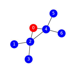
Figure 1: Communication Topology

In addition to the stability analysis, a simulation is included to provide empirical evidence of the controller performance. The scenario involves a network of $N=6$ servicer spacecraft tasked with tracking a single defunct spacecraft, simulating an approach and servicing operation. The communication topology governing the multi-spacecraft network is depicted in Fig. 1. The simulation spans a duration of 360 seconds.

Table 1: Spacecraft Parameters

Spacecraft Index	Mass (kg)	Cross-Sectional Area $(m^{2})$
$q_{0}$	10,000	1,000
$q_{1}$	640.1074	10.1267
$q_{2}$	1,087.4786	17.9324
$q_{3}$	25.1687	20.4416
$q_{4}$	470.9405	27.4020
$q_{5}$	241.4649	21.5405
$q_{6}$	161.1994	34.5757

The defunct spacecraft is initialized in a near-Earth elliptical orbit, characterized by a periapsis altitude of $300\times 10^{3}$ meters, an apoapsis altitude of $700\times 10^{3}$ meters, and an inclination angle $\frac{\pi}{6}$ radians. The semi-major axis, $a$, is calculated as the arithmetic mean of the periapsis and apoapsis altitudes. The initial orbital velocity is derived from the vis-viva equation, $v=\sqrt{\mu\left(\frac{2}{r_{\text{periapsis}}}-\frac{1}{a}\right)}$, where $\mu$ denotes the standard gravitational parameter of Earth.

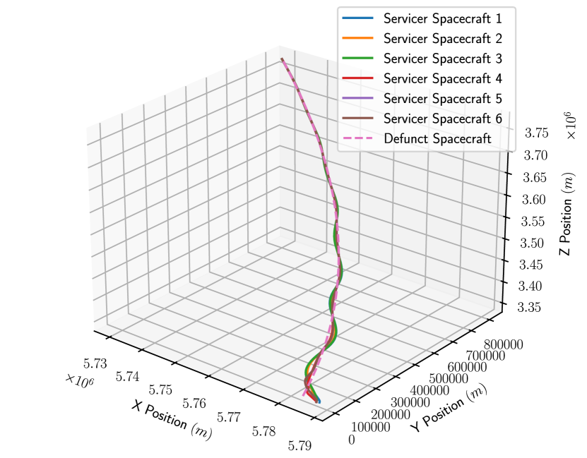
Figure 2: 3D visualization of the trajectories of all servicer spacecraft (solid lines) and the defunct spacecraft (dotted line). For visual clarity, only the first 60 seconds of the simulation.

The initial positions of the servicer spacecraft are offset from the defunct spacecraft’s initial conditions. These offsets are generated randomly, with radial distances uniformly distributed in the range $U\left(2500,5000\right)$ meters, and angular deviations in azimuth ($\gamma$) and elevation ($\phi$) sampled from $U\left(-0.5,0.5\right)$ radians. Each servicer spacecraft’s initial velocity matches the defunct spacecraft’s orbital velocity to ensure relative dynamics are dominated by initial positional offsets.

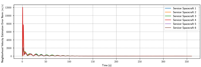
Figure 3: Plot showing the norm of the neighborhood velocity estimation error $\left(\left\|\tilde{\zeta}_{i}\right\|\right)$ over time for all servicer spacecraft.

Each servicer spacecraft employs an output matrix $C_{i}\in\mathbb{R}^{p_{i}\times 3}$, where the entries are uniformly sampled from $U\left(-2,2\right)$. The matrix row dimension, $p_{i}$, is randomly selected from $p_{i}\in\left\{1,2,3,4\right\}$. The specific matrices selected for this simulation are as follows:

$$C_{1} =\left[\begin{array}[]{ccc}1.5124&-1.8904&0.6818\end{array}\right],\ C_{2}=\left[\begin{array}[]{ccc}-0.2772&1.7565&1.1135\\ 0.8638&1.2110&-1.6287\end{array}\right],$$

$$C_{3} =\left[\begin{array}[]{ccc}1.5055&1.5784&-1.6598\\ -1.8437&-1.3206&1.5125\end{array}\right],\ C_{4}=\left[\begin{array}[]{ccc}0.3722&0.6866&-0.3528\\ -1.2097&-0.8414&-1.4315\\ 1.1332&-0.3498&-1.8633\end{array}\right],$$

$$C_{5} =\left[\begin{array}[]{ccc}1.9554&0.9926&-0.8782\\ 1.1571&-1.5870&-0.2084\\ 1.6343&-0.8255&-0.8488\end{array}\right],\ C_{6}=\left[\begin{array}[]{ccc}0.0991&-1.6655&1.6674\end{array}\right].$$

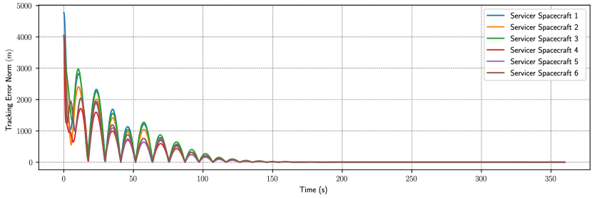
Figure 4: Plot showing the norm of the tracking error $\left(\left\|e_{i}\right\|\right)$ over time for all servicer spacecraft.

Each servicer spacecraft employs an Lb-DNN consisting of 4 hidden layers with 4 neurons per hidden layer. This configuration results in a total of 103 weights per spacecraft. The Lb-DNNs use the $\tanh$ activation function in the output layer, while the hidden layers employ the Swish activation function [38]. The weights are initialized using the Kaiming He initialization method [39] to leverage the Swish activation’s smooth approximation of the ReLU function. The control gains are selected as $k_{i}=0.65$ for $i\in\{1,\ldots,5\}$, $k_{6}=0.0001$, and $\Gamma_{i}=0.01\cdot I_{103}$ for $i\in\{1,\ldots,6\}$.

The dynamics governing the servicer and defunct spacecraft follow the nonlinear equations detailed in (4). For the servicer spacecraft, masses and cross-sectional areas are sampled from the uniform distributions $U\left(25,1500\right)\ kg$   and $U\left(1,50\right)\ m^{2}$, respectively. The properties of all spacecraft are listed in Table 1. The measurement model follows (10) and includes additive Gaussian noise with zero mean and a standard deviation of $\sqrt{0.5}$ meters.

A 3D visualization of the trajectories of all servicer spacecraft and the defunct spacecraft is shown in Fig. 2. The visualization is limited to the first 60 seconds of the simulation to provide a detailed view of the initial trajectory dynamics. This depiction illustrates the cooperative behavior of the servicer spacecraft as they maneuver within the operational region.

The performance of the neighborhood velocity estimation is shown in Fig. 3, which shows the norm of the estimation error $\left\|\tilde{\zeta}_{i}\right\|$ over time for all servicer spacecraft. The results indicate that all servicer spacecraft achieve steady-state estimation error values of approximately $5\ m/s$ after about 150 seconds. The initial transient spikes observed within the first 10 seconds are attributed to the zero-value initialization of the observer. This transient response could be mitigated by initializing the observer with prior estimates of the velocity, thereby improving the convergence characteristics.

The tracking performance of the servicer spacecraft is shown in Fig. 4, which shows the norm of the tracking error $\left\|e_{i}\right\|$ over time. The plot shows that all servicer spacecraft achieve steady-state tracking error values of approximately $5$ meters after approximately 200 seconds. This level of precision is considered sufficient to initiate servicing operations. The oscillatory behavior observed during the steady-state phase can be attributed to the choice of control gains. While adjustments to the gain parameters could reduce oscillations, such modifications would likely increase control effort, necessitating a trade-off between control performance and energy efficiency.

7 Conclusion

This work addresses challenges in spacecraft servicing by introducing a distributed state estimation and tracking framework that relies solely on relative position measurements and operates effectively under partial state information. The proposed $\rho$-filter reconstructs unknown states using locally available data, while a Lyapunov-based deep neural network adaptive controller compensates for uncertainties arising from unknown spacecraft dynamics. To ensure a well-posed collaborative spacecraft regulation problem, a trackability condition is established. Lyapunov-based stability analysis guarantees exponential error convergence in state estimation and spacecraft regulation to a neighborhood of the origin, contingent on this condition. Empirical validation is demonstrated through a simulation involving a network of six servicer spacecraft tasked with tracking a single defunct spacecraft. The servicer spacecraft achieve steady-state tracking errors of approximately 5 meters within 200 seconds, meeting precision requirements for initiating servicing operations.

Statements and Declarations

Funding

This research is supported in part by AFOSR grant FA9550-19-1-0169. Any opinions, findings, and conclusions or recommendations expressed in this material are those of the author(s) and do not necessarily reflect the views of the sponsoring agency.

Conflict of Interest

On behalf of all authors, the corresponding author states that there is no conflict of interest.

Consent for Publication

This work has been approved for public release: distribution unlimited. Case Number AFRL-2024-5871.

Code Availability

The code used in this study is available on request.

References

• \bibcommenthead
• [1] Guffanti, T. & D’Amico, S. Passively safe and robust multi-agent optimal control with application to distributed space systems. J. Guid. Control Dyn. 46, 1448–1469 (2023). URL https://doi.org/10.2514/1.G007207.
• [2] Arnas, D. & Linares, R. Uniform satellite constellation reconfiguration. J. Guid. Control Dyn. 45, 1241–1254 (2022). URL https://doi.org/10.2514/1.G006514.
• [3] Soderlund, A. A. & Phillips, S. Hybrid systems approach to autonomous rendezvous and docking of an underactuated satellite. J. Guid. Control Dyn. 46, 1901–1918 (2023). URL https://doi.org/10.2514/1.G006813.
• [4] Mercier, M. & Curtis, D. Optimal NMC trajectory design for on-orbit, multi-agent inspection missions. AIAA Scitech (2024). URL https://arc.aiaa.org/doi/abs/10.2514/6.2024-1867.
• [5] Bang, J. & Ahn, J. Multitarget rendezvous for active debris removal using multiple spacecraft. J. Spacecr. Rockets 56, 1237–1247 (2019). URL https://doi.org/10.2514/1.A34344.
• [6] Burch, J. L., Moore, T. E., Torbert, R. B. & Giles, B. L. Magnetospheric multiscale overview and science objectives. Space Science Reviews 199, 5–21 (2016).
• [7] Vaughan, M. et al. Towards persistent space observations through autonomous multi-agent formations. AIAA Scitech (2022). URL https://arc.aiaa.org/doi/abs/10.2514/6.2022-2074.
• [8] Asri, E. G. & Zhu, Z. H. Capturing an unknown uncooperative target with a swarm of spacecraft. AIAA Scitech (2024). URL https://arc.aiaa.org/doi/abs/10.2514/6.2024-0625.
• [9] Cho, H. & Kerschen, G. Satellite formation control using continuous adaptive sliding mode controller. AIAA/AAS Astrodyn. Spec. Conf. (2016). URL https://arc.aiaa.org/doi/abs/10.2514/6.2016-5662.
• [10] Kim, S.-G., Crassidis, J., Cheng, Y., Fosbury, A. & Junkins, J. Kalman filtering for relative spacecraft attitude and position estimation. AIAA Guid. Navig. Control Conf. (2012). URL https://arc.aiaa.org/doi/abs/10.2514/6.2005-6087.
• [11] Morgan, D. et al. Swarm-keeping strategies for spacecraft under J2 and atmospheric drag perturbations. J. Guid. Control Dyn. 35, 1492–1506 (2012). URL https://doi.org/10.2514/1.55705.
• [12] Sun, R., Wang, J., Zhang, D., Jia, Q. & Shao, X. Roto-translational spacecraft formation control using aerodynamic forces. J. Guid. Control Dyn. 40, 2556–2568 (2017).
• [13] Sun, X., Geng, C., Deng, L. & Chen, P. Geolocation of formation-flying spacecraft using relative position vector measurements. J. Guid. Control Dyn. 45, 764–773 (2022). URL https://doi.org/10.2514/1.G006377.
• [14] Zhang, K. & Demetriou, M. A. Adaptive neural network control of spacecraft rendezvous using nonlinear dynamical models in the presence of J2 perturbations. AIAA Guid. Navig. Control Conf. (2018). URL https://arc.aiaa.org/doi/abs/10.2514/6.2018-1105.
• [15] Harl, N., Rajagopal, K. & Balakrishnan, S. N. Neural network based modified state observer for orbit uncertainty estimation. J. Guid. Control Dyn. 36, 1194–1209 (2013). URL https://doi.org/10.2514/1.55711.
• [16] Park, T. H. & D’Amico, S. Adaptive neural-network-based unscented kalman filter for robust pose tracking of noncooperative spacecraft. J. Guid. Control Dyn. 46, 1671–1688 (2023). URL https://doi.org/10.2514/1.G007387.
• [17] Silvestrini, S. & Lavagna, M. R. Spacecraft formation relative trajectories identification for collision-free maneuvers using neural-reconstructed dynamics. AIAA Scitech (2020). URL https://arc.aiaa.org/doi/abs/10.2514/6.2020-1918.
• [18] LeCun, Y., Bengio, Y. & Hinton, G. Deep learning. Nature 521, 436–444 (2015).
• [19] Patil, O., Le, D., Greene, M. & Dixon, W. E. Lyapunov-derived control and adaptive update laws for inner and outer layer weights of a deep neural network. IEEE Control Syst Lett. 6, 1855–1860 (2022).
• [20] Patil, O. S., Le, D. M., Griffis, E. & Dixon, W. E. Deep residual neural network (ResNet)-based adaptive control: A Lyapunov-based approach, 3487–3492 (2022).
• [21] Nino, C. F., Patil, O. S., Philor, J., Bell, Z. & Dixon, W. E. Deep adaptive indirect herding of multiple target agents with unknown interaction dynamics, 2509–2514 (2023).
• [22] Hart, R., Patil, O., Griffis, E. & Dixon, W. E. Deep Lyapunov-based physics-informed neural networks (DeLb-PINN) for adaptive control design, 1511–1516 (2023).
• [23] Griffis, E., Patil, O., Hart, R. & Dixon, W. E. Lyapunov-based long short-term memory (Lb-LSTM) neural network-based adaptive observer. IEEE Control Syst. Lett. 8, 97–102 (2024).
• [24] Nino, C. F., Patil, O. S., Edwards, S. C., Bell, Z. I. & Dixon, W. E. Distributed target tracking under partial feedback using Lyapunov-based deep neural networks (2025).
• [25] Nino, C., Patil, O. & Dixon, W. E. Second-order heterogeneous multi-agent target tracking without relative velocities. IEEE Control Syst. Lett. 7, 3663–3668 (2023).
• [26] Griffis, E., Patil, O., Bell, Z. & Dixon, W. E. Lyapunov-based long short-term memory (Lb-LSTM) neural network-based control. IEEE Control Syst. Lett. 7, 2976–2981 (2023).
• [27] Schaub, H. & Junkins, J. Analytical Mechanics of Space Systems (AIAA Education Series, New York, 2003).
• [28] Vess, M. F. & Starin, S. R. A study on the effects of j2 perturbations on a drag-free control system for spacecraft in low earth orbit (NASA Goddard Space Flight Center, 2003).
• [29] Mostaza Prieto, D., Graziano, B. P. & Roberts, P. C. Spacecraft drag modelling. Prog. Aerosp. Sci. 64, 56–65 (2014).
• [30] Eggleston, J. M. & Dunning, R. S. Analytical evaluation of a method of midcourse guidance for rendezvous with earth satellites. National Aeronautics and Space Administration (1961). URL https://api.semanticscholar.org/CorpusID:128306715.
• [31] Kidger, P. & Lyons, T. Universal approximation with deep narrow networks. Proc. Mach. Learn. Res. (2020).
• [32] Lax, P. D. & Terrell, M. S. Multivariable Calculus with Applications (Springer International Publishing AG, 2017).
• [33] Zhang, F. Matrix Theory (Springer, 2011).
• [34] Lewis, F. L., Yegildirek, A. & Liu, K. Multilayer neural-net robot controller with guaranteed tracking performance. IEEE Trans. Neural Netw. 7, 388–399 (1996).
• [35] Fan, B., Yang, Q., Jagannathan, S. & Sun, Y. Asymptotic tracking controller design for nonlinear systems with guaranteed performance. IEEE Trans. Cybern. 48, 2001–2011 (2018).
• [36] M Krstic, P. K., I Kanellakopoulos. Nonlinear and Adaptive Control Design (John Willey, New York, 1995).
• [37] Horn, R. A. & Johnson, C. R. Matrix Analysis (Cambridge University Press., Cambridge, 1993).
• [38] Ramachandran, P., Zoph, B. & Le, Q. V. Swish: a self-gated activation function. arXiv: Neural Evol. Comput. (2017).
• [39] He, K., Zhang, X., Ren, S. & Sun, J. Delving deep into rectifiers: Surpassing human-level performance on imagenet classification. CoRR abs/1502.01852 (2015).