Stochastic Process Learning via Operator Flow Matching

Abstract

Expanding on neural operators, we propose a novel framework for stochastic process learning across arbitrary domains. In particular, we develop operator flow matching (OFM) for learning stochastic process priors on function spaces. OFM provides the probability density of the values of any collection of points and enables mathematically tractable functional regression at new points with mean and density estimation. Our method outperforms state-of-the-art models in stochastic process learning, functional regression, and prior learning.

1 Introduction

Stochastic processes are foundational to many domains, from functional regression and physics data assimilation, to financial markets, geophysics, and black box optimization. Stochastic processes can serve as prior distributions over functions and can provide the density of any finite collection of points. Conventionally, priors over processes are often hand-designed from predefined Gaussian processes (GP) and their variants tuned against data, only allowing for GP regression. This is despite the fact that phenomena modeled in the natural world often do not follow Gaussianity, Fig 1. Consequently, this hinders the flexibility and generalizability of these stochastic processes in real-world applications, leaving behind significant challenges for more general stochastic process learning (SPL).

In SPL, the prior over the stochastic process is learned from data, i.e., historical point evaluation of past experiments. Learning the prior over the process is crucial for universal functional regression (UFR), which is a recently proposed Bayesian scheme for functional regression and takes GP-regression as a special case when the prior is Gaussian (Shi et al., 2024a). UFR is important to scientific and engineering domains, including reanalysis, data completion-assimilation, uncertainty quantification, and black box optimization.

In this paper, we introduce a novel operator learning framework termed operator flow matching (OFM) for learning priors over stochastic processes through the joint distribution of any collection of points. To achieve this, we theoretically and empirically generalize marginal optimal transport flow matching (Tong et al., 2024) to infinite-dimensional function spaces where we map a GP into a prior over function spaces through a flow differential equation. We then derive SPL from the function space derivation and learn a prior over any collection of points. For SPL, we map any collection of pointwise evaluations of a GP to pointwise evaluations of target functions. This allows us to learn prior distributions over the more general stochastic process, hence enabling sampling values of any collection of points with their associated density and facilitating efficient UFR. We leverage this capability by extending neural operators Azizzadenesheli et al. (2024)–designed initially to map functions between infinite-dimensional spaces–to map between collections of points deploying their functional convergence properties. This serves as the essential architecture block in OFM.

After learning the prior and having access to the densities, OFM is used for UFR, where given any collection of points of the underlying function, we estimate the posterior mean value of any new collection of points and efficiently sample from their posterior values using stochastic gradient Langevin dynamics (SGLD) (Welling & Teh, 2011), i.e., a Gaussian sampling on the input GP space. We show that OFM outperforms state-of-the-art methods, including deep GPs, neural processes, and operator flows (OpFlow) (Salimbeni & Deisenroth, 2017; Jankowiak et al., 2020; Garnelo et al., 2018; Kim et al., 2019; Shi et al., 2024a).

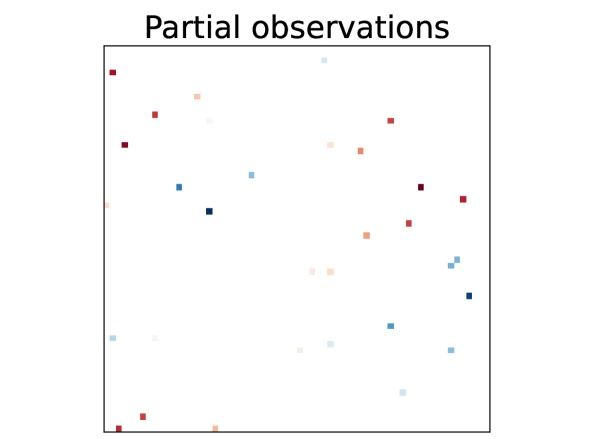
(a)

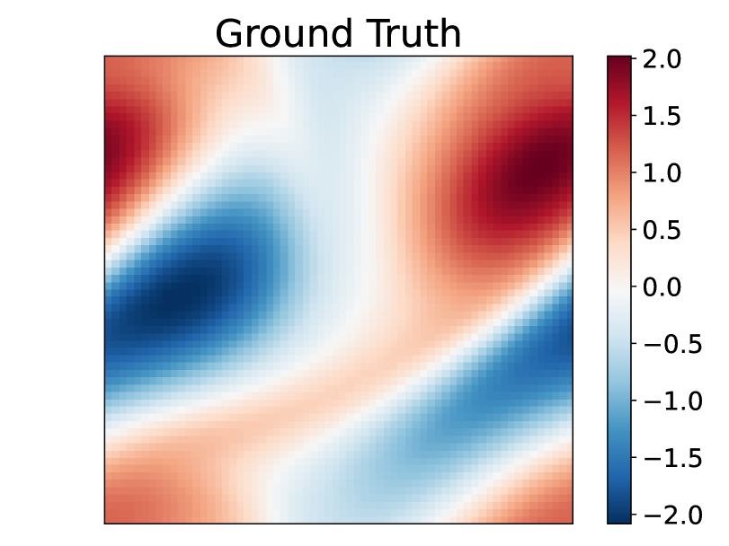
(b)

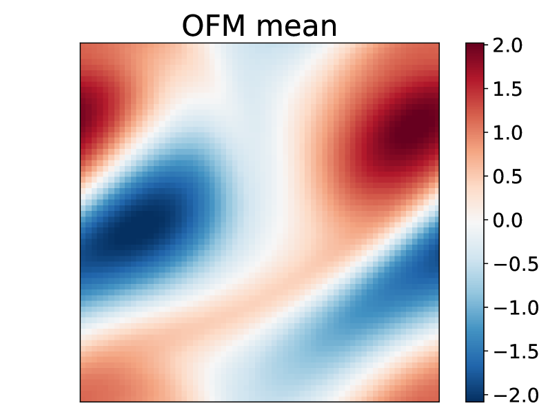
(c)

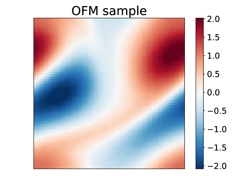
(d)

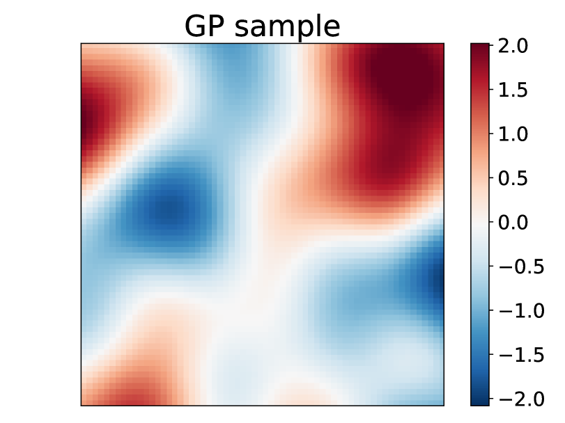
(e)

Figure 1: Operator Flow Matching (OFM) regression on Navier-Stokes functional data with resolution $64\times 64$. (a) 32 random observations. (b) Ground truth sample (c) Predicted mean from OFM. (d) One posterior sample from OFM. (e) One posterior sample from best fitted GP.

Our principal contribution is that OFM represents the first simulation-free continuous normalizing flow for functional regression purposes, which transports a GP to a target stochastic process and enables likelihood estimation for any collection of points. Compared with existing baselines in functional regression, OFM enjoys greater expressiveness without the architectural constraints seen in deep GPs or OpFlow, and avoids the theoretical limitations associated with neural processes (see Appendix A.11). We empirically show that regression with OFM outperforms existing baselines, matches classical GP regression on GP examples, and delivers exceptional performance on highly non-Gaussian functional datasets, such as those from Navier-Stokes equations and black hole simulations.

2 Related work

Neural operators. Neural operators constitute a paradigm in machine learning for learning maps between function spaces, a generalization of conventional neural networks that map between finite dimensional spaces (Li et al., 2021; Kovachki et al., 2023). Among neural operator architectures, Fourier neural operators (FNO) (Li et al., 2021) enable convolution in the spectral domain and are effective for operator learning (Pathak et al., 2022; Wen et al., 2023; Yang et al., 2021; 2023; Sun et al., 2023; Li et al., 2023). In this work, we use this as our choice of neural operators architecture.

Direct function samples. There is a body of work on generative models dedicated to learning distributions over functions, such that direct sampling on the function space is possible. For example, generative adversarial neural operators (GANO) generalize generative adversarial nets on finite dimensional spaces to function spaces (Rahman et al., 2022; Shi et al., 2024b), yielding a neural operator generative model that maps GP to data functions (Azizzadenesheli et al., 2024). Other works in this area have followed the success of diffusion models (Song et al., 2021; Ho et al., 2020) in finite dimensional spaces, e.g., denoising diffusion operators generalize diffusion models to function spaces by using GP as a means to add noise and use neural operators to learn the score operator on function-valued data (Lim et al., 2023; Pidstrigach et al., 2023; Kerrigan et al., 2023a). Moreover, the same principle has been deployed to generalize flow matching (Lipman et al., 2023) to functional spaces (Kerrigan et al., 2023b), an approach closely related to our work. However, these works on learning generative models on function spaces do not support UFR the way GP-regression does because they (i) focus solely on generating function samples, (ii) do not clarify how to model a stochastic process on point value sequential generation, and (iii) do not provide point evaluation of probability density.

Stochastic processes. Earlier works on SPL have focused on hand-tuned methods in the style of GP-regression. In these cases, an expert tunes the GP parameters given a set of experimental samples. More advanced methods rely on deep GPs, in which a network of GPs is stacked on top of each other. The parameters of deep GPs are commonly optimized by minimizing the variational free energy, which serves as a bound on the negative log marginal likelihood. (Damianou & Lawrence, 2013; Liu et al., 2020). Deep GPs have limitations in terms of learnability, expressivity, and computational complexity. Warped GPs  (Kou et al., 2013) and transforming GP (Maroñas et al., 2021) methods use historical data to learn a pointwise transformation of GP values and achieve on par performance compared to deep GP type methods. The pointwise nature of such approaches limits their generality.

Another attempt to address SPL is neural processes (Garnelo et al., 2018), inspired by variational inference method and designed for sampling from function spaces. This method trains a model to map any collection of points and their values to a vector, used as an input to a decoder that maps any collection of points to their values. The architectures used in these modes are not consistent as the number of points grows, and same with the decoder, making the approach limited to finite dimensions. The diffusion based variants (Dutordoir et al., 2023) also use uncorrelated Gaussian noise, and the results do not exist in function spaces (Rahman et al., 2022; Lim et al., 2023). In the end, methods based on neural processes are unable to provide density estimation for collections of points, as needed for UFR and SPL in general.

Finally, OpFlow introduced invertible neural operators that are trained to map any collection of points sampled from a GP to a new collection of points in the data space (Shi et al., 2024a), using the maximum likelihood principle. This method is consistent as the resolution grows, captures the likelihood of any collection of points, and allows for UFR using SGLD. However, similar to normalizing flow (Papamakarios et al., 2021) methods in finite dimensional domains, the use of invertible deep learning models makes their training a challenge, particularly with regards to expressiveness, as also described in the original OpFlow work.

3 Operator Flow Matching

Here, we introduce the problem setting and the notations used for OFM in function space. We recommend that readers consult Appendix A.1–A.3 for a foundational overview of SPL and UFR. Subsequently, we present the framework of OFM, which extends marginal optimal transport flow matching (Tong et al., 2024) to infinite-dimensional spaces. We further demonstrate the generalization of flow matching to stochastic processes as it is induced from OFM on function spaces. Finally, we illustrate how to evaluate exact and tractable likelihoods for any point evaluation of functions using OFM, making it applicable in the UFR setting.

For a real separable Hilbert space $(\mathcal{H},\langle\cdot,\cdot\rangle,\lVert\cdot\rVert)$, equipped with the Borel $\sigma-$ algebra of measurable sets denoted by $\mathcal{B(H)}$, we introduce two measures on $\mathcal{B(H)}$, $\nu_{0}$ as the reference measure and $\nu_{1}$ as the data measure. Consider a function $h_{0}$ sampled from $\nu_{0}$, such that $h_{0}\sim\nu_{0}$. For a smooth time-varying infinite dimensional vector field $\mathcal{G}_{t}:\mathcal{H}\rightarrow\mathcal{H}$, we define an ordinary differential equation (ODE)

$$\frac{\partial\Phi_{t}(h_{0})}{\partial t}=\mathcal{G}_{t}(\Phi_{t}(h_{0})),$$ (1)

with initial condition $\Phi_{0}(h_{0})=h_{0}$, where $h=h_{t}=\Phi_{t}(h_{0})$ represents a function $h_{0}$ transported along a vector field from time $0$ to time $t$. The diffeomorphism $\Phi_{t}$ induces a pushforward measure $\mu_{t}:=[\Phi_{t}]_{\sharp}(\mu_{0})$, with $\mu_{0}=\nu_{0}$, and we refer to $\mu_{t}$ as the path of probability measure. The goal is to construct a path of probability measure such that at $t=1$, $\mu_{1}\approx\nu_{1}$. The dynamic relationship between the time varying measure $\mu_{t}$ and vector field $\mathcal{G}_{t}$ can be characterized by the continuity equation:

$$\frac{\partial\mu_{t}}{\partial t}=-\nabla\cdot(\mu_{t}\mathcal{G}_{t})$$ (2)

In practice, we use Eq. 2 in its weak form (Ambrosio et al., 2008; Kerrigan et al., 2023b) to check whether a given vector field $\mathcal{G}_{t}$ generates the target $\mu_{t}$:

$$\int_{0}^{1}\int_{\mathcal{H}}\frac{\partial\varphi(h,t)}{\partial t}+\langle\mathcal{G}_{t}(h),\nabla_{h}\varphi(h,t)\rangle)d\mu_{t}(h)dt=0,~~~\forall\varphi\in\text{Cyl}(\mathcal{H}\times[0,1])$$ (3)

Where $\text{Cyl}(\mathcal{H}\times[0,1])$ is the space of smooth cylindrical test functions. Suppose that the time-varying vector field $\mathcal{G}_{t}$ and induced $\mu_{t}$, which satisfy Eq.3, are known. We parameterize $\mathcal{G}_{t}$ with a neural operator $\mathcal{G}_{\theta}:[0,1]\times\mathcal{H}\rightarrow\mathcal{H}$ and regress $\mathcal{G}_{\theta}$ to target $\mathcal{G}_{t}$ through flow matching objective.

$$\mathcal{L}_{\text{FM}}^{\dagger}=\mathbb{E}_{t\sim\mathcal{U}[0,1],h\sim\mu_{t}}\lVert\mathcal{G}_{\theta}(t,h)-\mathcal{G}_{t}(h)\rVert^{2}$$ (4)

However, similar to its finite-dimensional counterpart, $\mathcal{G}_{t}$ is typically unknown. Moreover, there are infinitely many paths of probability measures that satisfy the Eq. 3 and ensure $\mu_{1}\approx\nu_{1}$. Therefore, it is necessary to specify a path of probability measures to effectively guide the learning of $\mathcal{G}_{\theta}$.

3.1 Conditional probability measures and Gaussian measures

Consider a joint probability measure $\pi(\nu_{0},\nu_{1})$ on $\mathcal{H\times H}$, where the reference measure $\nu_{0}$, is chosen as a Gaussian measure, whose absolute continuity is well-studied (Bogachev, 1998). We characterize $\nu_{0}$ by a GP with trace-class covariance operator. e.g. $\nu_{0}=\mathcal{N}(m_{0},C_{0})$, where $m_{0}$ is the mean, $C_{0}$ is the covariance operator. With the joint measure $\pi(\nu_{0},\nu_{1})$, we sample a function pair $z:=(h_{0},h_{1})$.

Assuming $\nu_{1}$ has full support on the Cameron-Martin space associated with $\nu_{0}$, we construct a conditional probability measure $\mu_{t}(\cdot|z)$ as a Gaussian measure with trace-class covariance operator and small operator norm to approximate Dirac measures in the sense of weak convergence. Such that, at $t=0$ and $t=1$, $\mu_{t}(\cdot|z)$ is a centered around $h_{0},h_{1}$, approximating $\delta_{h_{0}},\delta_{h_{1}}$ respectively; Subsequently, we can construct a new marginal probability measure by mixing these approximated Dirac measures:

$$\mu_{t}(A)=\int\mu_{t}({A|z})d\pi(z),~\forall A\in\mathcal{B(H)}$$ (5)

Due to $d\pi(z)$ being always positive, the conditional probability measure (Dirac measure approximated by Gaussian measure) is absolutely continuous with respect to $\mu_{t}$. Eq. 5 indicates that $\mu_{0}=\int\delta_{h_{0}}d\pi(z)\approx\nu_{0}$, and $\mu_{1}=\int\delta_{h_{1}}d\pi(z)\approx\nu_{1}$. This formulation suggests that $\mu_{0},\mu_{1}$ represent convolutions of $\nu_{0},\nu_{1}$ with Gaussian measures. For a more detailed discussion on convolution with Gaussian measures, we refer the readers to Appendix B.1 of  Lim et al. (2023).

Suppose $\int_{0}^{1}\int_{\mathcal{H}}\int_{\mathcal{H\times H}}\lVert\mathcal{G}_{t}(h|z)\rVert d\mu_{t}(h|z)d\pi(z)dt$ is finite to guarantee the vector field is sufficiently regular, where $\mathcal{G}_{t}(\cdot|z)$ is the conditional vector field. Under this condition, the vector field that generates $\mu_{t}$ as specified in Eq. 5 and Eq. 3 can be expanded as follows :

$$\mathcal{G}_{t}(h)=\int_{\mathcal{H\times H}}\mathcal{G}_{t}(h|z)\frac{d\mu_{t}(\cdot|z)}{d\mu_{t}}(h)d\pi(z)$$ (6)

Eq. 6 is an extension of the Theorem 1 as detailed in Kerrigan et al. (2023b), and we provide the derivation in Appendix A.5. We note that $\mu_{t}(\cdot|z)$ is a Gaussian measure and can be expressed as $\mu_{t}(\cdot|z)=\mathcal{N}(m_{t},C_{t})$, with mean $m_{t}$ and trace-class covariance operator $C_{t}$. Inspired by Tong et al. (2024), we choose $m_{t}$ and $C_{t}$ to have the following forms:

$$m_{t}=t\cdot h_{1}+(1-t)\cdot h_{0}$$ (7)

$$C_{t}=\sigma_{\text{min}}^{2}C_{0}$$ (8)

where $C_{0}$ is the same Gaussian covariance operator defined for $\nu_{0}$ and $\sigma_{\text{min}}$ is a small constant. Further, similar to finite-dimensional flow matching, we only consider the simplest vector field that applies a canonical transformation for Gaussian measures, such that the flow has the form: $\Phi_{t}(h_{0}|z)=m_{t}+\sigma_{\text{min}}h_{0}\approx t\cdot h_{1}+(1-t)\cdot h_{0}$. From Eq. 1, we can get $\mathcal{G}_{t}(h|z)=h_{1}-h_{0}$, indicating $\mathcal{G}_{t}(h|z)$ is independent of the time $t$ and the path from $h_{0}$ to $h_{1}$ is a direct, straight line. Equipped with well-constructed conditional vector field and probability measures, we can train a neural operator $\mathcal{G}_{\theta}$ with the conditional flow matching loss

$$\mathcal{L}_{\text{CFM}}^{\dagger}=\mathbb{E}_{t\sim\mathcal{U}[0,1],h\sim\mu_{t},z\sim\pi(\nu_{0},\nu_{1})}\lVert\mathcal{G}_{\theta}(t,h)-\mathcal{G}_{t}(h|z)\rVert^{2}.$$ (9)

Next, we explore how to approximate the true optimal transport plan from optimal coupling of the joint measure $\pi(\nu_{0},\nu_{1})$. A common way for measuring the distance between two probability measure is 2-Wasserstein distance, which a special case of static Kantorovich formulation (Kantorovich & Rubinshtein, 1958). The static 2-Wasserstein distance is defined as follows

$$W_{\text{sta}}(\nu_{0},\nu_{1})^{2}_{2}=\inf_{\pi\in\Pi}\int_{\mathcal{H\times H}}\lVert h_{0}-h_{1}\rVert^{2}d\pi(h_{0},h_{1})$$ (10)

In the ODE framework, we also care about the dynamic form of the 2-Wasserstein distance to estimate the cost along the transport trajectory, which also is a special case of dynamic Kantorovich formulation (Chizat et al., 2018).

$$W_{\text{dyn}}(\nu_{0},\nu_{1})_{2}^{2}=\inf_{\mu_{t},\mathcal{G}_{t}}\int_{\mathcal{H}}\int_{0}^{1}\lVert\mathcal{G}_{t}(h)\rVert^{2}d\mu_{t}(h)dt$$ (11)

Within the OFM framework, the marginal probability measure is a sum of Dirac measures as described in Eq. 5, and we selected $\nu_{0}$ as a Gaussian measure and assumed $\nu_{1}$ has full support on the Cameron-Martin space associated with $\nu_{0}$. Furthermore, the cost function of 2-Wasserstein distance is squared $L^{2}$ norm, which is continuous by nature. According to Theorem 4.3 and Lemma 4.4 of Chizat et al. (2018), $W_{\text{sta}}=W_{\text{dyn}}$ for our specifically constructed $\mu_{t}$ and $\mathcal{G}_{t}$ in the sense of weak convergence. Therefore, to get the dynamic optimal transport plan, we only need to find a joint measure $\pi(\nu_{0},\nu_{1})$ that achieves the infimum in Eq. 10. In practice, we use a minibatch approximation of optimal coupling between $\nu_{0}$ and $\nu_{1}$. The above approach extends the dynamic (marginal) optimal transport framework of (Tong et al., 2024) to infinite-dimensional function space. The related work of Kerrigan et al. (2024) addresses a similar problem, but from a different perspective. For a detailed comparison, please refer to Appendix A.11. In the next subsection, we show how to generalize flow matching to stochastic process, which is induced from the function space derivation.

3.2 Generalizing Flow matching to stochastic processes

Stochastic processes are inherently infinite-dimensional, and define distribution over any collection of points ((Brémaud, 2020), Chapter 5.1). We generalize the above marginal optimal transport flow matching on function spaces to stochastic process by defining the transport map on any collection of points. We then show that this generalization recovers infinite-dimensional flow matching implemented with neural operator as the collection of points covers the space in the limit.

For any $n$, and points $\{x_{1},x_{2},\ldots,x_{n}\}$, consider an ODE system in which a vector of random variables $u_{0}\in\mathbb{R}^{n}$ is gradually transformed into $u_{1}$, for which, the $i$th entry is equal to $u(x_{i})$, via a smooth, time-varying vector field, denoted by $\mathcal{G}_{t}$ with abuse of notation.

$$u_{t}:=\Phi_{t}(u_{0})=u_{0}+\int_{0}^{t}\mathcal{G}_{s}(u_{s})ds.$$ (12)

Given the collection of points and the density of $p_{0}:=p_{0}\left(\{u_{0}(x_{1}),u_{0}(x_{2}),\ldots,u_{0}(x_{n})\}\right)=\mathcal{N}\left(\textbf{0},K\left(\{x_{1},x_{2},\ldots,x_{n}\}\right)\right)$, where $K$ is a $n\times n$ covariance matrix with entries described by kernel function $k(x_{i},x_{j})$ and $u_{0}\sim p_{0}$, the time-varying density $p_{t}$ induced by the diffeomorphism $\Phi_{t}$ or $\mathcal{G}_{t}$ can be computed using the well-known transport equation  (Lipman et al., 2023; Fjelde et al., 2024),

$$\frac{\partial p_{t}(u_{t})}{\partial t}=-(\nabla\cdot(\mathcal{G}_{t}p_{t}))(u_{t})$$ (13)

Eq. 13 shows that constructing $p_{t}$ is equivalent to constructing $\mathcal{G}_{t}$ for finite entries for which the analysis carries to finite collection of random variables. In the following, we refer to $p_{t}$ as the marginal probability path induced by $\mathcal{G}_{t}$ for the given collection of points. From Eq. 13, the log density can be computed through integration,

$$\log p_{t}(u_{t})=\log p_{0}(u_{0})-\int_{0}^{t}(\nabla\cdot\mathcal{G}_{s})(u_{s})ds.$$ (14)

In this formulation, we are seeking a specific vector field that transports density $q_{0}$ to target density $q_{1}$ for any $n$ and any collection of points $\{x_{1},x_{2},\ldots,x_{n}\}$ with boundary conditions $p_{0}=q_{0},p_{1}=q_{1}$. We propose to extend optimal transport flow matching (Tong et al., 2024) to stochastic processes and parameterize a potential vector field $\mathcal{G}_{t}$ with a neural operator $\mathcal{G}_{\theta}$, which can be optimized through the flow matching objective for SPL,

$$\mathcal{L}_{\text{FM}}(\theta):=\sup_{n}\sup_{\{x_{1},x_{2},\ldots,x_{n}\}}\mathbb{E}_{t\sim\mathcal{U}(0,1),u_{t}\sim p_{t}}\lVert\mathcal{G}_{\theta}(t,u_{t})-\mathcal{G}_{t}(u_{t})\rVert^{2}$$ (15)

Note that $p_{t}$ and $u_{t}$ depend on the point collocations. In the above equation, the suprema are intractable and we replace them with expectation as a soft approximation. Moreover, the true $\mathcal{G}_{t}$ is usually unknown and to address it, one can derive a probability path conditioned on latent variable $z$ of the same alphabet size as the collection. Consequently, the marginal probability path $p_{t}(u_{t})$ is a mixture of conditional probability paths $p_{t}(u_{t}|z)$,

$$p_{t}(u_{t})=\int p_{t}(u_{t}|z)q(z)dz$$ (16)

$$\mathcal{G}_{t}(u_{t})=\mathbb{E}_{q(z)}[\frac{\mathcal{G}_{t}(u_{t}|z)p_{t}(u_{t}|z)}{p_{t}(u_{t})}].$$ (17)

Given Eq. 17, the conditional flow matching (CFM) objective is defined as

$$\mathcal{L}_{\text{CFM}}(\theta):=\mathbb{E}_{n}\mathbb{E}_{x_{1},x_{2},\ldots,x_{n}}\mathbb{E}_{t,q(z),p_{t}(u_{t}|z)}\rVert\mathcal{G}_{\theta}(t,u_{t})-\mathcal{G}_{t}(u_{t}|z)\rVert^{2}$$ (18)

Equations 15, when suprema are replaced with expectations, and 18 have identical gradient for $\theta$, which indicates $\nabla_{\theta}\mathcal{L}_{\text{FM}}(\theta)=\nabla_{\theta}\mathcal{L}_{\text{CFM}}(\theta)$. Inspired by the finite dimensional developments (Tong et al., 2024), the variable $z$ is chosen as a couple $(u_{0},u_{1})$ from the the coupling $\pi(u_{0},u_{1})$, where mini-batch optimal transport plan is achieved via minimizing the dynamic 2-Wasserstein distance, which is equivalent to the static 2-Wasserstein distance under mild conditions on $\mathbb{R}^{n}$ with

$$W_{\text{dyn}}(q_{0},q_{1})_{2}^{2}=\inf_{p_{t},\mathcal{G}_{t}}\int_{\mathbb{R}^{n}}\int_{0}^{1}p_{t}(u_{t})\lVert\mathcal{G}_{t}(u_{t})\rVert^{2}du_{t}dt$$ (19)

$$W_{\text{sta}}(q_{0},q_{1})^{2}_{2}=\inf_{\pi\in\Pi}\int_{\mathbb{R}^{n}\times\mathbb{R}^{n}}\lVert u_{1}-u_{0}\rVert^{2}d\pi(u_{0},u_{1})$$ (20)

Considering the class of Gaussian conditional probability paths $p_{t}(u_{t}|z)=\mathcal{N}(u_{t}|m_{t}(z),\sigma_{t}(z)^{2}K\left(\{x_{1},x_{2},\ldots,x_{n}\}\right))$, with conditional flow $\Phi_{t}(u_{0}|z)=\sigma_{t}u_{0}+m_{t}$. Specially, we choose $m_{t}=tu_{1}+(1-t)u_{0}$ and $\sigma_{t}=\sigma$, where $\sigma>0$ is a small constant. Then we can derive a closed-form expression for the corresponding vector field (Tong et al., 2024). Detailed derivation provided in Appendix A.4

$$\mathcal{G}_{t}(u_{t}|z)=u_{1}-u_{0}$$ (21)

With the aforementioned developments, for any collection of points, we transport a Gaussian distribution to a target distribution. The Gaussian distribution is drawn from a GP, with its covariance matrix $K({x_{1},\cdots,x_{n}})$ determined by the kernel function $k(x_{i},x_{j})$ of the GP. According to Kolmogorov extension theorem (KET) (Kolmogorov & Bharucha-Reid, 2018), there exists a valid stochastic process whose finite-dimensional marginal is the pushforward distribution under $\mathcal{G}_{\theta}$. This demonstrates that the generalization of flow matching to infinite-dimensional spaces with neural operators naturally induces the generalization of flow matching to stochastic processes. In the scenario where the limit of points covers the space, these two become equivalent. For a detailed explanation and proof, please refer to Appendix A.1 and A.2.

Recent work on finite-dimensional flow matching (Tong et al., 2024) has shown benefits of model training and generation quality with the optimal transport plan. We have extended this approach to any collection of points and the infinite-dimensional space. It is reasonable to assume that similar advantages would apply in these contexts as well; however, a thorough investigation into why the optimal transport plan should be preferred is beyond the scope of this paper. In addition, the theory development for generalizing flow matching to stochastic process as well as the development of optimal transport infinite-dimensional flow matching are considered as additional contributions of this paper.

3.3 Likelihood estimation and Bayesian Universal Functional Regression

We parameterize $\mathcal{G}_{\theta}$ with FNO (Li et al., 2021) to ensure our model is resolution agnostic, and assume $\mathcal{G}_{\theta}$ learns the map from $\nu_{0}$ to $\nu_{1}$, which serves as the prior. In practice, we deal with discretized evaluations of functions that may have different sampling rate and resolution. For instance, consider a function $u$ sampled from $\nu_{1}$, observed on a collection of points $u_{1}:=\{u(x_{1}),u(x_{2}),...,u(x_{m})\}$; thus we have a density function $\mathbb{P}(u_{1})$ defined on collection of points $\{x_{1},x_{2},...,x_{m}\}$, where $\mathbb{P}(u_{1})$ is derived from measure $\nu_{1}$. This is similar to how a multivariate Gaussian distribution can be derived from a Gaussian measure characterized by a Gaussian process. Therefore, we can rewrite Eq. 14 as:

$$\log\mathbb{P}(u_{1})=\log\mathbb{P}(u_{0})-\int_{0}^{1}(\nabla\cdot\mathcal{G}_{\theta})(u_{t})dt,$$ (22)

where $u_{0}$ is drawn from the reference Gaussian measure $\nu_{0}$, which is also defined on the collection of point $\{x_{1},x_{2},...,x_{m}\}$. Thus $\mathbb{P}(u_{0})$ is a multivariate Gaussian with a tractable density function. Furthermore, with the probability density function $\mathbb{P}(u_{1})$, we can evaluate the precise likelihood of any $u_{1}$ from $\mathbb{P}(u_{1})$ via Eq. 22. However, following a similar argument to Grathwohl et al. (2018), the computation of $\nabla\cdot\mathcal{G}_{\theta}(u)$ incurs a cost of $\mathcal{O}(m^{2})$ where $m$ is cardinality of set $\{x_{1},x_{2},...,x_{m}\}$. This quadratic time complexity renders the likelihood calculation prohibitively expensive. To address this issue, we adopt the strategy proposed in Grathwohl et al. (2018), utilizing the unbiased Skilling-Hutchinson trace estimator (Hutchinson, 1989; Skilling, 1989) to approximate the divergence term. This technique reduces the computation cost to $\mathcal{O}(m)$, which is the same as the cost of inference, thereby streamlining the evaluation process. The estimator is implemented as follows:

$$\nabla\cdot\mathcal{G}_{\theta}(u)=\mathbb{E}_{p(\varepsilon)}[\varepsilon^{T}\frac{\partial\mathcal{G}_{\theta}(u,t)}{\partial u}\varepsilon]$$ (23)

In the unbiased trace estimator, the random variable $\varepsilon$ is characterized by $\mathbb{E}(\varepsilon)=0$ and $\text{Cov}(\varepsilon)=I$. This estimator benefits from the optimal transport nature of the map which gives rise to a direct line. The gradient computation in Eq. 23 can be efficiently handled with reverse-mode automatic differentiation, allowing for precise estimation with arbitrary error by averaging over a sufficient number of runs, which can benefit from parallel computing of GPUs.

With the efficient tool established for estimating the likelihood of any discretized function samples, we now turn our attention to UFR, i.e., a Bayesian functional regression. Consider a collection of pointwise observations of the underlying unknown function drawn from $\nu_{1}$, that is corrupted with Gaussian noise, denoted as $\{\widehat{u}(x_{1}),\widehat{u}(x_{2}),\ldots,\widehat{u}(x_{n})\}$ or $\{\widehat{u}(x_{i})\}_{i=1}^{n}$. We specifically focus on Gaussian white noise characterized by $\epsilon\sim\mathcal{N}(0,\sigma^{2})$, such that $\widehat{u}(x_{i})=u(x_{i})+\epsilon_{i}$ for $i\in\{1,\cdots,n\}$ (depending on the nature of the problem, the noise may also be considered as a correlated GP noise). In UFR setting, we are interested in the posterior distribution over new $m\geq n$ points that include the $n$ observation points. With Bayes rule, we have the posterior:

$$\mathbb{P}\left(\{u(x_{i})\}_{i=1}^{m}\Big{|}\{\widehat{u}(x_{i})\}_{i=1}^{n}\right)=\frac{\mathbb{P}\left(\{\widehat{u}(x_{i})\}_{i=1}^{n}\Big{|}\{u(x_{i})\}_{i=1}^{m}\right)\cdot\mathbb{P}\left(\{u(x_{i})\}_{i=1}^{m}\right)}{\mathbb{P}\left(\{\widehat{u}(x_{i})\}_{i=1}^{n}\right)}$$ (24)

Taking the logarithm of Eq. 24, we have:

$$\log\mathbb{P}\left(\{u(x_{i})\}_{i=1}^{m}\Big{|}\{\widehat{u}(x_{i})\}_{i=1}^{n}\right)=\log\mathbb{P}\left(\{\widehat{u}(x_{i})\}_{i=1}^{n}\Big{|}\{u(x_{i})\}_{i=1}^{m}\right)+\log\mathbb{P}\left(\{u(x_{i})\}_{i=1}^{m}\right)\\ -\log\mathbb{P}\left(\{\widehat{u}(x_{i})\}_{i=1}^{n}\right)$$ (25)

Given $\epsilon_{i}\sim\mathcal{N}(0,\sigma^{2})$ and $\{\epsilon_{i}\}_{i=1}^{n}$ is a multivariate Gaussian, then $\{\widehat{u}(x_{i})\}_{i=1}^{n}\Big{|}\{u(x_{i})\}_{i=1}^{n}$ is a shifted multivariate Gaussian with mean $\{u(x_{i})\}_{i=1}^{n}$ translated from the original multivariate Gaussian $\{\epsilon_{i}\}_{i=1}^{n}$. Due to the translation invariance property of Gaussian distribution, We have :

$$\log\mathbb{P}\left(\{\widehat{u}(x_{i})\}_{i=1}^{n}\Big{|}\{u(x_{i})\}_{i=1}^{n}\right)=\log\mathbb{P}\left(\{\epsilon_{i}\}_{i=1}^{n}\right)=-\frac{\sum_{i=1}^{n}\lVert\widehat{u}(x_{i})-u(x_{i})\rVert^{2}}{2\sigma^{2}}-\frac{n}{2}\log(2\pi\sigma^{2})$$ (26)

We notice $m>n$ and $\{\widehat{u}(x_{i})\}_{i=i}^{n}$ only depends on $\{u(x_{i})\}_{i=1}^{n}$, and doesn’t depend on $\{u(x_{i})\}_{i=n+1}^{m}$. Thus $\log\mathbb{P}\left(\{\widehat{u}(x_{i})\}_{i=1}^{n}\Big{|}\{u(x_{i})\}_{i=1}^{m}\right)=\log\mathbb{P}\left(\{\widehat{u}(x_{i})\}_{i=1}^{n}\Big{|}\{u(x_{i})\}_{i=1}^{n}\right)$.

For evaluating $\log\mathbb{P}\left(\{u(x_{i})\}_{i=1}^{m}\right)$, which is the second part on the right-hand side of Eq. 25, we can efficiently calculate it with the likelihood estimation tool described above. The third part on the right hand side of Eq. 25 ($\log\mathbb{P}\left(\{\widehat{u}(x_{i})\}_{i=1}^{n}\right)$) represents the evidence and is constant. Thus the posterior distribution of Eq 25 can be simplified as:

$$\log\mathbb{P}\left(\{u(x_{i})\}_{i=1}^{m}\Big{|}\{\widehat{u}(x_{i})\}_{i=1}^{n}\right)=-\frac{\sum_{i=1}^{n}\lVert\widehat{u}(x_{i})-u(x_{i})\rVert^{2}}{2\sigma^{2}}+\log\mathbb{P}\left(\{u(x_{i})\}_{i=1}^{m}\right)+C$$ (27)

Where the constant $C=-\frac{n}{2}\log(2\pi\sigma^{2})-\log\mathbb{P}\left(\{\widehat{u}(x_{i})\}_{i=1}^{n}\right)$. Given the closed-form posterior distribution, we adopt SGLD (Welling & Teh, 2011) to efficiently sample from the posterior, and then derive statistical features of interest, e.g. mean, maximum a posteriori, and posterior uncertainty, i.e., variance, from the posterior samples. More specifically, we follow the posterior sampling strategy developed by Shi et al. (2024a), which suggests that given an invertible framework, sampling within the input GP space (where the Gaussian measure $\nu_{0}$ is defined) and then mapping to the data function space (where data measure $\nu_{1}$ is defined) yields better performance compared to direct sampling in the data function space. In all experiments, we use the dopri5 ODE solver provided by torchdiffeq Chen et al. (2019) with atol=1e-5 and rtol=1e-5. Detailed posterior sampling algorithm is provided in Appendix A.8

4 Experiments

In this section, we demonstrate the superior regression performance compared to several baselines across a variety of function datasets, including both Gaussian and highly non-Gaussian Process. As baselines, we employ standard GP Regression (Williams & Rasmussen, 2006), Deep GPs (Salimbeni & Deisenroth, 2017; Jankowiak et al., 2020), Neural Processes (Kim et al., 2019; Garnelo et al., 2018), and OpFlow (Shi et al., 2024a).

For our function datasets, we analyze: (1) Gaussian and non-Gaussian with known posterior, including 1D GPs, 2D GPs, and 1D Truncated GPs, (TGP). (2) Highly non-GPs, datasets with unknown posterior, such as those derived from Navier-Stokes equations (Li et al., 2021), black hole dataset from expensive Monte Carlo simulation, and 2D Signed Distance Functions extracted from MNIST digits (MNIST-SDF) (Sitzmann et al., 2020). During regression, we assume that the prior $\mathcal{G}_{\theta}$ is always successfully trained and remains frozen. Details about the learning process for priors and experimental setup for regression are provided in the Appendix A.9,  A.10.

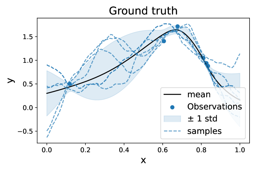
(a)

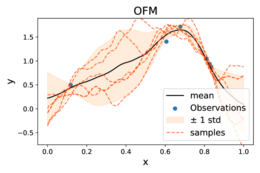
(b)

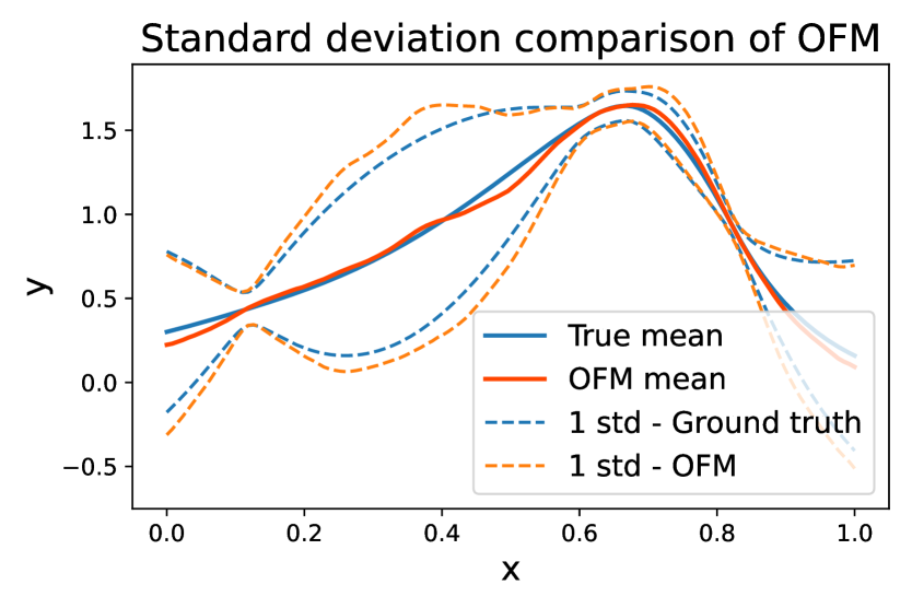
(c)

Figure 2: OFM regression on GP data. (a) Ground truth GP regression with observed data and predicted samples. (b) OFM regression with observed data and predicted samples. (c) Standard deviation comparison between true GP and OFM predictions.

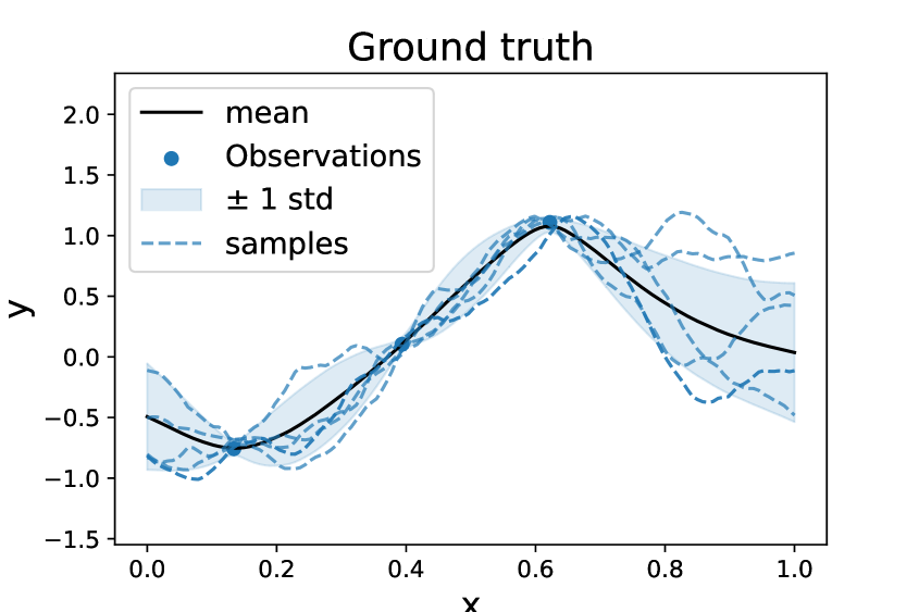
(a)

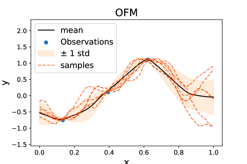
(b)

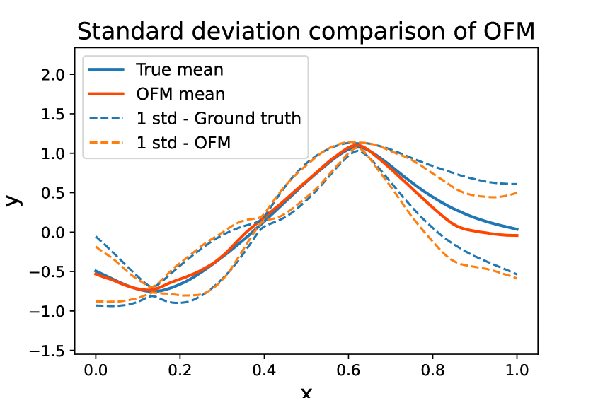
(c)

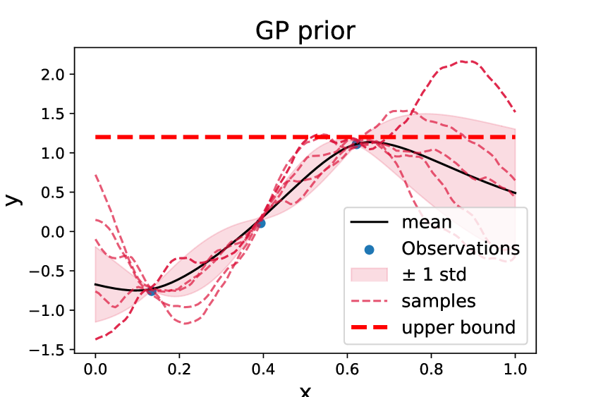
(d)

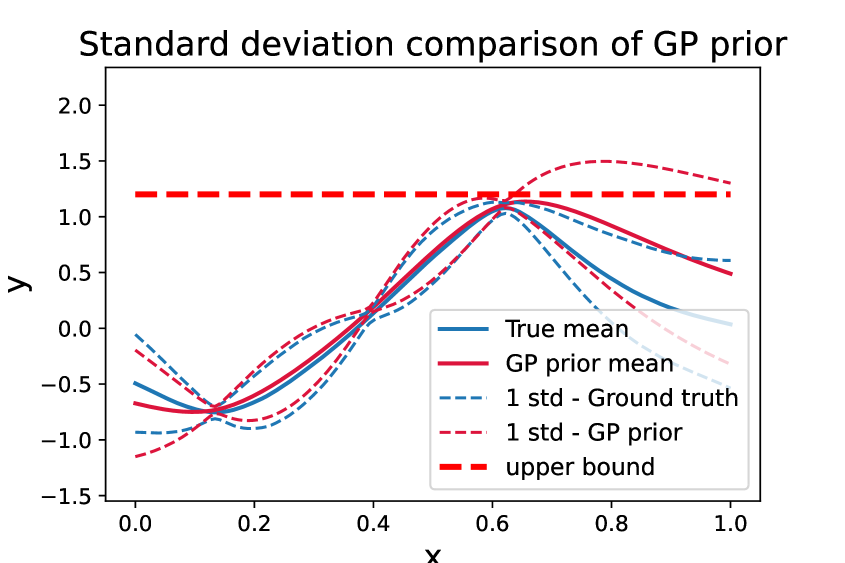
(e)

Figure 3: OFM regression on TGP data. (a) Ground truth TGP regression with observed data and predicted samples. (b) OFM regression with observed data and predicted samples. (c) Standard deviation comparison between true TGP and OFM predictions. (d) Prior GP regression with observed data and predicted samples. (e) Standard deviation comparison between true TGP and GP prior predictions.

1D GP data. This experiment replicates the results of classical GP regression, wherein the posterior distributions are precisely known in a closed form. The process involves generating a single new realization from the data measure $\nu_{1}$. We then select observations at $6$ randomly chosen positions, incorporating a predefined noise level. The posterior is inferred across 128 positions, which includes estimating noise-free values at the observation points. We evaluate our results with two commonly used quantities in the GP literature (1) Standardized Mean Squared Error (SMSE) that normalizes the mean squared error by the variance of the ground truth; and (2) Mean Standardized Log Loss (MSLL), originally introduced by  Williams & Rasmussen (2006), defined as:

$$-\log p(\{u(x_{i})\}_{i=1}^{m}|\{\widehat{u}(x_{i})\}^{n}_{i=1})=\frac{1}{2}\log(2\pi\sigma^{2}_{*})+\frac{(\{u(x_{i})\}_{i=1}^{m}-\{\bar{u}(x_{i})\}_{i=1}^{m})^{2}}{2\sigma^{2}_{*}}$$ (28)

where $\{\widehat{u}(x_{i})\}^{n}_{i=1}$ represents observations, $\{x_{i}\}_{i=1}^{m},\{u(x_{i})\}_{i=1}^{m},$ indicate the new positions queried, and the test data (true posterior samples). Meanwhile, $\{\bar{u}(x_{i})\}_{i=1}^{m},\sigma^{2}_{*}$ are predicted mean and variances from the model. We average out SMSE and MSLL over a test dataset contains 1000 true GP posterior samples for all models. The performance of each model is detailed in Table 1. From Fig. 2, the regression with OFM matches the analytical solution very well and provides realistic posterior samples.

Truncated GP data. In this experiment, we analyze the regression performance of OFM for tractable non-GP. Specifically, we work on truncated GP (Swiler et al., 2020; Shi et al., 2024a), which constrains the function amplitude within a specified range. This is achieved by applying a sampling-rejection strategy on samples from the GP prior. We set the bounds of our TGP to $[-1.2,1.2]$ and perform regression using observations only at three points, while estimating the posterior across 128 points. Subsequently, we sample 1000 true TGP posteriors from the GP prior to calculate the mean and standard deviation. Traditional metrics like MSLL and SMSE, which assume a Gaussian posterior, are not suitable for TGP. Therefore, we evaluate performance using the mean squared error for both the predicted mean and standard deviation. The results are reported in Table. 1, and illustrated in Fig. 3. OFM accurately learns the specified bounds and provides accurate estimations of mean and standard deviation, along with realistic posterior samples. In contrast, directly applying GP regression exceeds the bounds and yields unrealistic posterior samples.

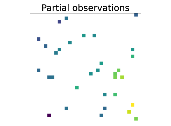
(a)

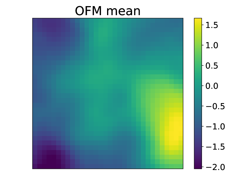
(b)

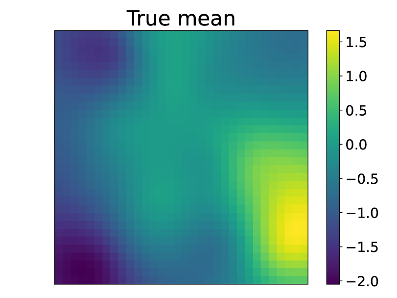
(c)

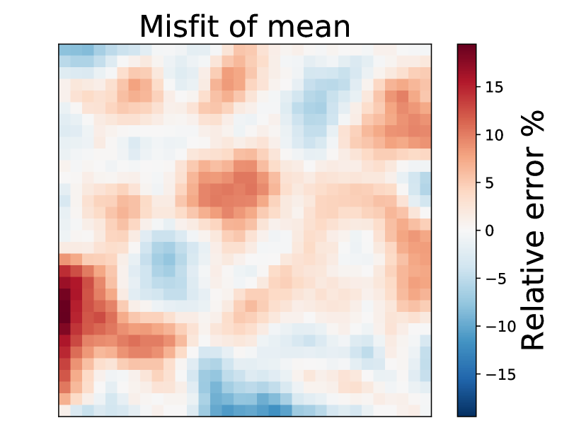
(d)

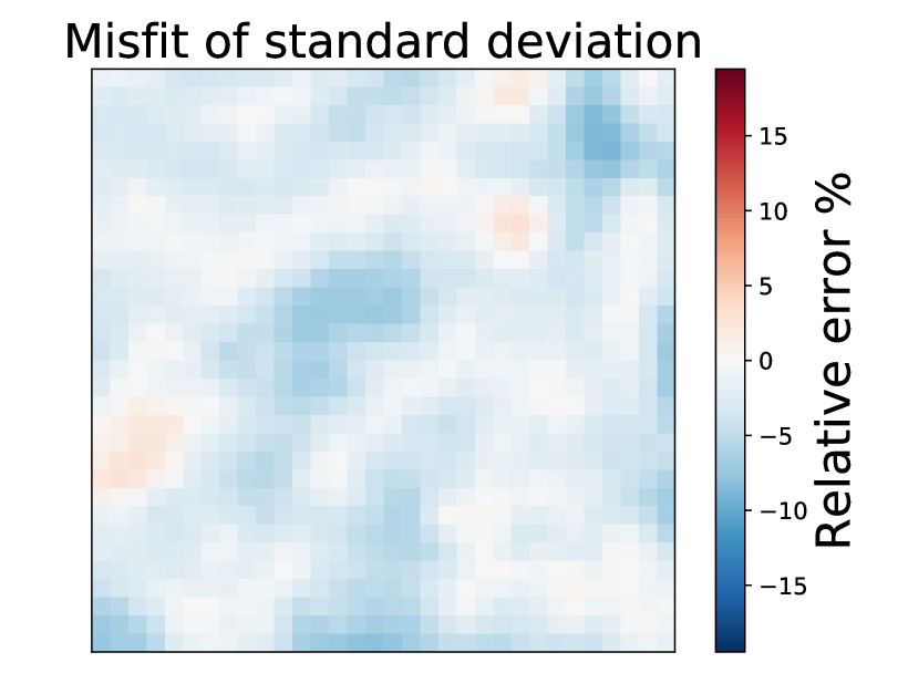
(e)

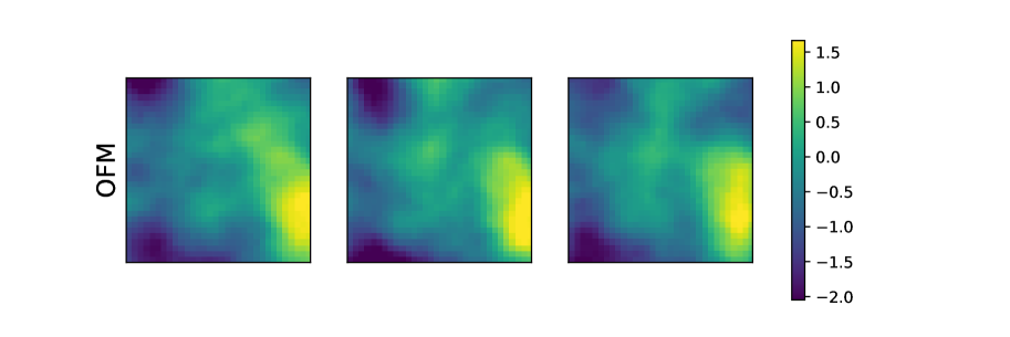
(f)

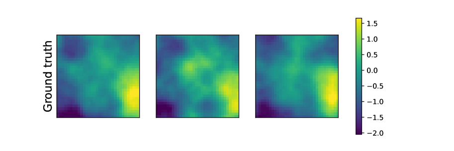
(g)

Figure 5: OFM regression on 2D GP data with resolution 32$\times$32. (a) 32 random observations. (b) Predicted mean from OFM. (c) Ground truth mean from GP regression. (d) Misfit of the predicted mean. (e) Misfit of predicted standard deviation. (f) Predicted samples from OFM. (g) Predicted samples from GP regression.

2D GP data. Similar to the 1D GP example, we extend our regression analysis to 2D GP data. As shown in Fig.  5 and detailed in Table 1, OFM provide accurate posterior estimation. The relative error shown in Fig.  5 is the absolute error normalized by the maximum absolute value of the mean prediction derived from the ground truth GP regression.

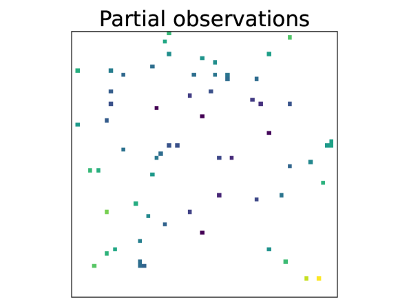
(a)

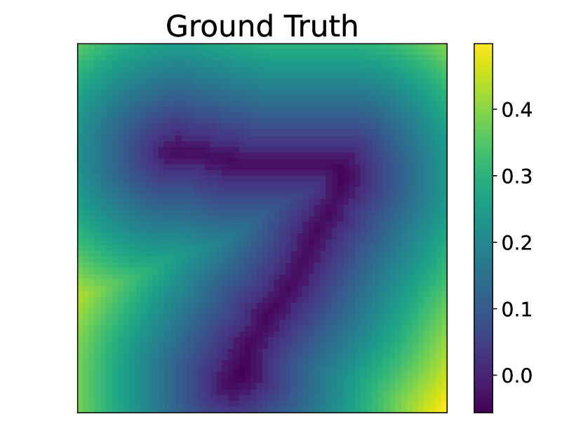
(b)

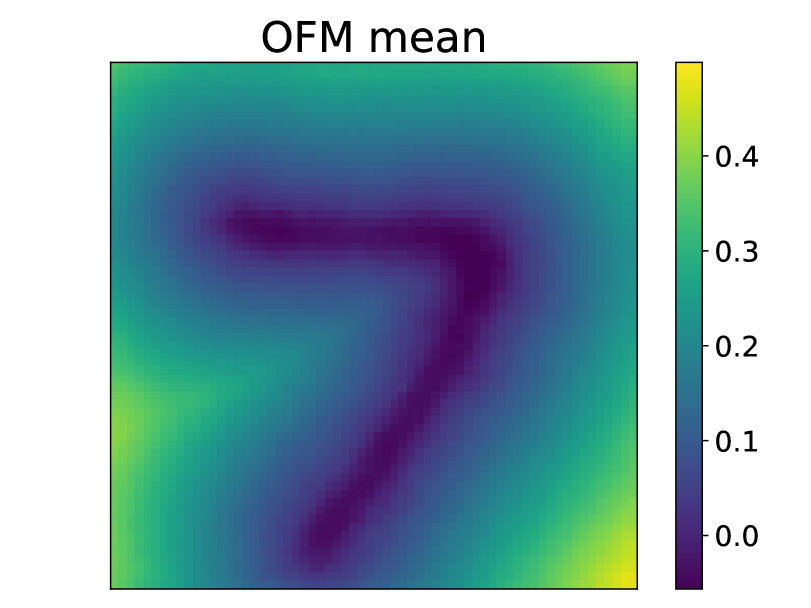
(c)

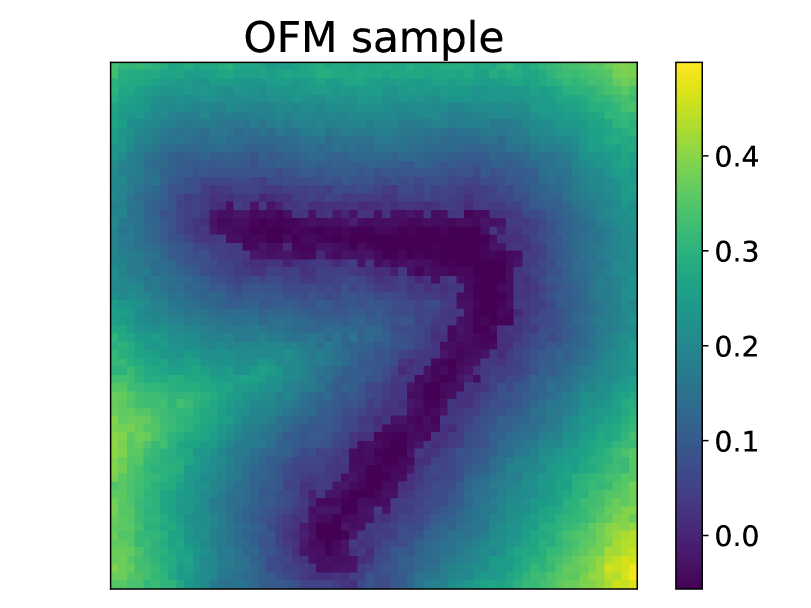
(d)

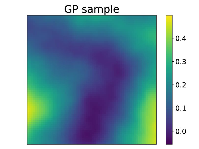
(e)

Figure 7: OFM regression on MNIST-SDF with resolution $64\times 64$. (a) 64 random observations. (b) Ground truth sample. (c) Predicted mean from OFM. (d) One posterior sample from OFM. (e) One posterior sample from best fitted GP.

Navier-Stokes, Black hole and MNIST-SDF datasets. We collected a 2D Navier-Stokes dataset and applied OFM for the regression. Unlike the GP experiments, where MSLL and SMSE score serve as standard benchmarks, evaluating the performance of models on general non-GPs presents a significant challenge due to the difficulty of determining the true posterior and lack of benchmarks. Therefore, we present the predicted mean, and a posterior sample in Fig  1 for visual comparison with the ground truth. The predicted mean, along with the posterior sample, are closely aligned with the ground truth. In contrast, traditional GP regression failed to accurately capture the dynamics of the Navier-Stokes data. In Fig. 4, we conduct a similar analysis using a simulated black hole dataset. Here, OFM provides a more realistic mean and posterior sample that capture the density and swirling patterns of the black hole. Once again, GP regression fails to capture these key statistics. Next, we observe similar outcomes when applying OFM to the MNIST-SDF example (Fig 7), where OFM correctly recognizes the number "$7$" while GP regression does not.

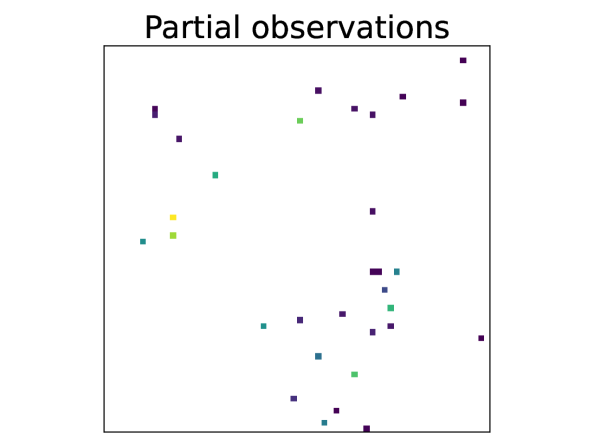
(a)

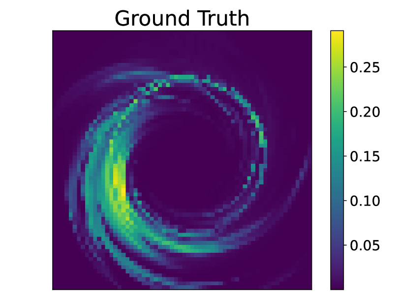
(b)

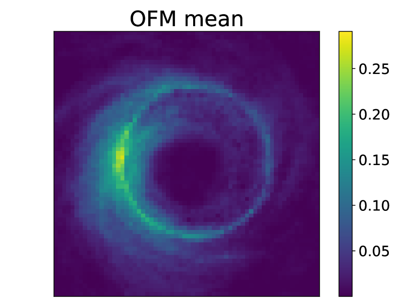
(c)

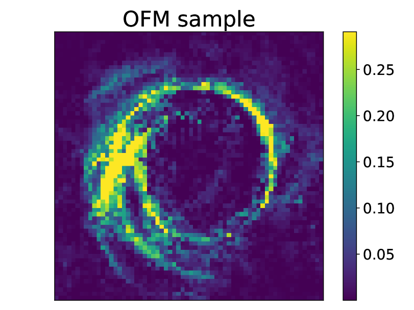
(d)

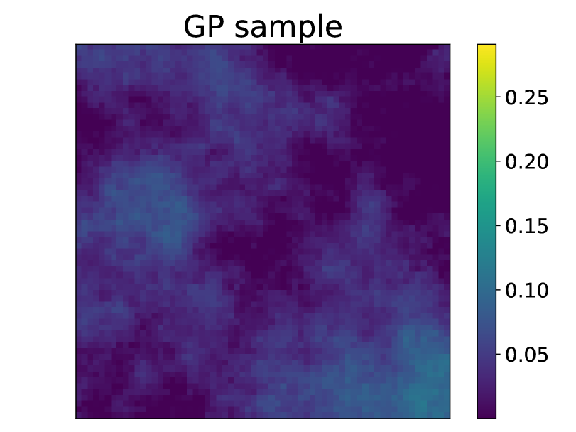
(e)

Figure 4: OFM regression on black hole data with resolution $64\times 64$. (a) 32 random observations. (b) Ground truth sample. (c) Predicted mean from OFM. (d) One posterior sample from OFM. (e) One posterior sample from best fitted GP.

Dataset $\rightarrow$	1D GP		2D GP		1D TGP
Algorithm $\downarrow$ Metric $\rightarrow$	SMSE	SMLL	SMSE	SMLL	$\mu$	$\sigma$
GP prior	-	-	-	-	$6.4\cdot 10^{-2}$	$1.6\cdot 10^{-2}$
OpFlow	$5.0\cdot 10^{-1}$	$2.0\cdot 10^{-1}$	$1.4\cdot 10^{-1}$	$\mathbf{1.1\cdot 10^{-1}}$	$1.3\cdot 10^{-2}$	$3.9\cdot 10^{-3}$
NP	$6.1\cdot 10^{-1}$	$4.5\cdot 10^{~0}$	$1.7\cdot 10^{-1}$	$2.1\cdot 10^{~0}$	$1.0\cdot 10^{-1}$	$1.9\cdot 10^{-2}$
ANP	$5.1\cdot 10^{-1}$	$9.8\cdot 10^{-1}$	$1.6\cdot 10^{-1}$	$1.1\cdot 10^{~0}$	$1.4\cdot 10^{-1}$	$1.7\cdot 10^{-2}$
DGP	$4.1\cdot 10^{-1}$	$6.8\cdot 10^{-2}$	$1.8\cdot 10^{~0}$	$4.2\cdot 10^{~0}$	$4.9\cdot 10^{-1}$	$1.4\cdot 10^{-2}$
DSPP	$4.7\cdot 10^{-1}$	$6.5\cdot 10^{~0}$	$1.9\cdot 10^{-1}$	$6.6\cdot 10^{~0}$	$1.1\cdot 10^{-2}$	$1.3\cdot 10^{-2}$
OFM	$\mathbf{4.1\cdot 10^{-1}}$	$\mathbf{5.5\cdot 10^{-2}}$	$\mathbf{1.3\cdot 10^{-1}}$	$1.6\cdot 10^{-1}$	$\mathbf{5.2\cdot 10^{-3}}$	$\mathbf{9.5\cdot 10^{-4}}$

Table 1: Comparison of OFM with baseline models: GP regression; OpFlow (Shi et al., 2024a); Neural Processes ( Garnelo et al. (2018), NP); Attentive NP ( Kim et al. (2019), ANP); Deep variational GP ( Salimbeni & Deisenroth (2017), DGP); Deep Sigma Point Process ( Jankowiak et al. (2020), DSSP); Datasets contain 1D GP, 2D GP, and 1D TGP examples. Metrics SMSE and SMLL used for 1D GP and 2D GP example. Mean squared error for the predicted mean $(\mu)$ and predicted standard deviation ($\sigma$) are used for TGP example. Performance of GP regression for 1D GP and 2D GP are removed (marked with ’$-$’), which are taken as the ground truth. Best performance in bold.

5 Conclusion

In this paper, we proposed Operator Flow Matching (OFM) for stochastic process learning, which generalizes flow matching models to infinite-dimensional space and stochastic process with optimal transport path. OFM efficiently computes the probability density for any finite collection of points and supports mathematically tractable functional regression. We extensively tested OFM across a diverse range of datasets, including those with closed-form GP and non-GP data, as well as highly non-GP such as Navier-Stokes and black hole data. In comparative evaluations, OFM consistently outperformed all baseline models, establishing new standards in stochastic process learning and regression 

Acknowledgments

This material is based upon work supported by the U.S. Department of Energy, Office of Science, Office of Advanced Scientific Computing Research, Science Foundations for Energy Earthshot under Award Number DE-SC0024705. We also wish to thank Charles Gammie, Ben Prather, Abhishek Joshi, Vedant Dhruv, and Chi-kwan Chan for providing the black hole simulations.

Appendix A Appendix

A.1 Stochastic process learning

Let $(\Omega,\mathcal{F},P)$ denote a probability space and let $(\mathbb{R}^{d},\mathcal{B}(\mathbb{R}^{d}))$ denote a measurable space where $\mathcal{B}(\mathbb{R})$ is the Borel space. Following the standard definition of stochastic processes (Brémaud (2020), Chapter 5.1), a stochastic process $\mathcal{P}$ on a domain $D$ is a collection of $\mathbb{R}^{d}$-valued random variables indexed by members of $D$, i.e.,

$$\{a(x):x\in D\}$$

jointly following the probability law $P$. In the special case of Gaussian processes, e.g., Wiener process, following the Gaussian law for $P$, for any collection points $\{x_{1},x_{2},\ldots,x_{n}\}$, the random variables $\{a(x_{1}),a(x_{2}),\ldots,a(x_{n})\}$ are jointly Gaussian, resulting in a function $a$ to be drawn from a GP. We need to emphasize, $\{a(x_{1}),a(x_{2}),\ldots,a(x_{n})\}$ is a collection of random variables (random vector) equipped with Lebesgue measure, and represents a discretized observation of one continuous function $a$. In practice, the joint probability distribution of the collection of the random variables is unknown a priori, and needs to be learned.

In SPL, one way we suggest is to learn an invertible operator $\mathcal{T}$ that maps a base stochastic process $\mathcal{P}$ to another stochastic process $\mathcal{Q}$ that represents the data via discretization convergence theorem (see Appendix A.2). That is, for any collection of points $\{x_{1},x_{2},\ldots,x_{n}\}$, and for any $n$, the operator $\mathcal{T}$ maps the law on $\{a(x_{1}),a(x_{2}),\ldots,a(x_{n})\}$ to $\{u(x_{1}),u(x_{2}),\ldots,u(x_{n})\}$ and vice versa for the inverse $\mathcal{T}^{-1}$, where $u(x)$ is a pointwise evaluation of function data sample, i.e.,

$$\{u(x_{1}),u(x_{2}),\ldots,u(x_{n})\}=\mathcal{T}\left(\{a(x_{1}),a(x_{2}),\ldots,a(x_{n})\}\right)\par$$

Then, the probability of $\{u(x_{1}),u(x_{2}),\ldots,u(x_{n})\}$, at evaluation points $\{x_{1},x_{2},\ldots,x_{n}\}$, for any $n$ and collection of points on $D$ is given by,

$$\mathbb{P}\left(\{u(x_{1}),u(x_{2}),\ldots,u(x_{n})\}\right) =\textbf{J}\mathcal{T}\Big{|}_{\{a(x_{1}),a(x_{2}),\ldots,a(x_{n})\}}\mathbb{P}\left(\{a(x_{1}),a(x_{2}),\ldots,a(x_{n})\}\right)$$

where with abuse of notation $\mathbb{P}(u(x))$ denotes the density of $u(x)$ at point $x$, same for $\mathbb{P}(a(x))$, and similarly, following the notation in Theorem $11.1$ of Villani (2009), $\textbf{J}\mathcal{T}\Big{|}_{\{a(x_{1}),a(x_{2}),\ldots,a(x_{n})\}}$ is the absolute value of the Jacobian determinant of the map from the random vector $\{a(x_{1}),a(x_{2}),\ldots,a(x_{n})\}$ at points $\{x_{1},x_{2},\ldots,x_{n}\}$ to the random vector $\{u(x_{1}),u(x_{2}),\ldots,u(x_{n})\}$  via inverse operator $\mathcal{T}^{-1}$. We further show that the pushedforward $\mathcal{Q}$ is indeed a valid stochastic process via Kolmogorov Extension Theorem (KET) (Kolmogorov & Bharucha-Reid, 2018) with a proof provided in Appendix. A.2 . In SPL, we aim to learn a neural operator $\mathcal{T}_{\theta}$ such that the resulting $\mathcal{Q}$ matches the data process under the true $\mathcal{T}$.

A.2 Model stochastic process with infinite-dimensional flow matching via kolmogorov Extension Theorem

In operator learning, neural operators (Li et al., 2021; Kovachki et al., 2023; Azizzadenesheli et al., 2024) are typically designed to map an input function to an output function. When the input function is provided at a specific discretization (e.g., a set of points with their corresponding values), the model processes this discretized input as a collection of points and their values. Traditionally, in operator learning, this process is seen as an approximation of the operator’s application to the underlying continuous function, where the discretization introduces approximation errors. Thus, the input is conceptually still treated as a function.

Moreover, the application of the operator to a collection of points is well-defined, and, by the discretization convergence theorem, as the number of points increases, this operation converges to a well-defined mapping. In this paper, leveraging these properties, we adopt a different perspective as described in the introduction. We extend neural operators to define explicit maps between collections of points. In this framework, the input is not the abstract function itself but rather a collection of points and their associated values. Importantly, this mapping remains well-defined regardless of the number of points in the collection and, by the discretization convergence theorem, converges to a unique mapping as the point collection approaches the underlying continuous function.

Next, we show that given an invertible operator $\mathcal{T}$ and a valid stochastic process $\mathcal{P}$ whose finite dimensional marginal is $\mathbb{P}(\{a(x_{1}),a(x_{2}),...,a(x_{n})\}$, there exist a valid stochastic process $\mathcal{Q}$ with finite-dimensional marginal $\{u(x_{1}),u(x_{2}),\ldots,u(x_{n})\}.$

Once again, as defined in Section A.1

$$\{u(x_{1}),u(x_{2}),\ldots,u(x_{n})\}=\mathcal{T}\left(\{a(x_{1}),a(x_{2}),\ldots,a(x_{n})\}\right)$$

Then, the probability of $\{u(x_{1}),u(x_{2}),\ldots,u(x_{n})\}$, at evaluation points $\{x_{1},x_{2},\ldots,x_{n}\}$, for any $n$ and collection of points on $D$ is given by,

$$\mathbb{P}\left(\{u(x_{1}),u(x_{2}),\ldots,u(x_{n})\}\right)=\textbf{J}\mathcal{T}\Big{|}_{\{a(x_{1}),a(x_{2}),\ldots,a(x_{n})\}}\mathbb{P}\left(\{a(x_{1}),a(x_{2}),\ldots,a(x_{n})\}\right)$$ (29)

where with abuse of notation $\mathbb{P}(u(x))$ denotes the density of $u(x)$ at point $x$, same for $\mathbb{P}(a(x))$, and similarly, following the notation in Theorem $11.1$ of Villani (2009), $\textbf{J}\mathcal{T}\Big{|}_{\{a(x_{1}),a(x_{2}),\ldots,a(x_{n})\}}$ is the absolute value of the Jacobian determinant of the map from the random vector Jacobian of the map from the random vector $\{a(x_{1}),a(x_{2}),\ldots,a(x_{n})\}$ at points $\{x_{1},x_{2},\ldots,x_{n}\}$ to the random vector $\{u(x_{1}),u(x_{2}),\ldots,u(x_{n})\}$ via inverse operator $\mathcal{T}^{-1}$. We should notice Eq. 29 represents the changes of variables between two random vectors, with Lebesgue measure involved. The connection between the finite-dimensional marginal (equipped with Lebesgue measure) and the probability measure of a stochastic process in infinite-dimensional space is described by Kolmogorov Extension theorem (KET) (Kolmogorov & Bharucha-Reid, 2018), which assures that if all finite-dimensional distributions (i.e., distributions of function at finite collection of points) are consistent, then a stochastic process exists that matches finite-dimensional distributions.

Formally, according to KET, to establish that a valid stochastic process $\mathcal{Q}$, which has $\mathbb{P}\left(\{u(x_{1}),u(x_{2}),\ldots,u(x_{n})\}\right)$ as its finite dimensional distributions, it is essential to demonstrate that such a joint distribution satisfies the following two consistency properties:

Permutation invariance. For any permutation $\pi$ of $\{1,\cdots,n\}$, the joint distribution should remain invariant when elements of $\{x_{1},\cdots,x_{n}\}$ are permuted, such that

$$\mathbb{P}\left(\{u(x_{1}),u(x_{2}),\ldots,u(x_{n})\}\right)=\mathbb{P}\left(\{u(x_{\pi(1)}),u(x_{\pi(2)}),\ldots,u(x_{\pi(n)})\}\right)$$ (30)

Marginal Consistency. This principle specifies that that if a portion of the set is marginalized, the marginal distribution will still align with the distribution defined on the original set, such that for $m\geq n$

$$\mathbb{P}\left(\{u(x_{1}),u(x_{2}),\ldots,u(x_{n})\}\right)=\int\mathbb{P}\left(\{u(x_{1}),u(x_{2}),\ldots,u(x_{m})\}\right)du(x_{n+1})\cdots du(x_{m})$$ (31)

The permutation invariance property is naturally upheld when utilizing operator, as there is no inherent order among the elements in the set $\{x_{1},x_{2},\ldots,x_{n}\}$. Furthermore, the marginal consistency property is also maintained due to the definition of operator $\mathcal{T}$ (see Eq. 29), which ensures that $\mathbb{P}\left(\{u(x_{1}),u(x_{2}),\ldots,u(x_{n})\}\right)$ is closed under marginalization. This is because $\mathbb{P}\left(\{a(x_{1}),a(x_{2}),\ldots,a(x_{n})\}\right)$ is closed under marginalization, which fully determines $\mathbb{P}\left(\{u(x_{1}),u(x_{2}),\ldots,u(x_{n})\}\right)$ through the Jacobian. While verifying that $\mathcal{Q}$ constitutes a valid induced stochastic process is straightforward given the $\mathcal{T}$, approximating the $\mathcal{T}$ with a neural operator is non-trivial and depends highly on the model used. For instance, in Transforming GP (Maroñas et al., 2021), the authors employ a marginal normalizing flow, which acts as a point-wise operator to transform values from a GP to another. Consequently, the induced Jacobian is a diagonal matrix. More recently, OpFlow (Shi et al., 2024a) introduces an invertible neural operator by generalizing RealNVP to function space, which induces a triangular Jacobian matrix. In our work, we extend this framework to a more comprehensive case: a diffeomorphism. Here, the induced Jacobian is a full-rank matrix and is not necessarily triangular or diagonal, the determinant of the Jacobian for any collection of points is calculated through Eq 22.

Last, we want to clarify the the connection between the notions of operator $\mathcal{T}$ and operator $\mathcal{G}$ throughout this paper. The operator $\mathcal{T}$ is the $\Phi_{t}$ (a diffeomporhism) defined in Eq. 12, which is the integral of $\mathcal{G}$ over time interval $[0,1]$. Due to the nature of an ODE system, $\mathcal{T}$ is invertible. However, $\mathcal{G}$ is not necessary invertible, which enables us to parameterize it with a classical neural operator, like FNO (Li et al., 2021).

A.3 Universal Functional Regression

UFR is concerned with Bayesian regression on function spaces (Shi et al., 2024a), where it can be used to infer the posterior of an unknown function on a domain $D$ from a collection of pointwise observations. The observations are often corrupted with noise of variance $\sigma^{2}$, denoted as $\{\widehat{u}(x_{1}),\widehat{u}(x_{2}),\ldots,\widehat{u}(x_{n})\}$ or $\{\widehat{u}(x_{i})\}_{i=1}^{n}$. More specifically, for $m\geq n$ points at which the function is to be inferred,

$$\mathbb{P}\left(\{u(x_{1}),u(x_{2}),\ldots,u(x_{m})\}\Big{|}\{\widehat{u}(x_{1}),\widehat{u}(x_{2}),\ldots,\widehat{u}(x_{n})\}\right)$$

Note that when the prior over the function space is Gaussian, UFR reduces to the celebrated GP regression. Following Bayes rule, and maps between stochastic processes, we obtain the log posterior as follows,

$$\log\mathbb{P}\left(\{u(x_{i})\}_{i=1}^{m}\Big{|}\{\widehat{u}(x_{i})\}_{i=1}^{n}\right)= -\frac{1}{2}\sum_{i}^{n}\frac{\left(\widehat{u}(x_{i})-u(x_{i})\right)^{2}}{\sigma^{2}}-n\log(\sigma)-\frac{n}{2}\log(2\pi)$$

$$+\log\mathbb{P}\left(\{u(x_{i})\}_{i=1}^{m}\right)-\log\mathbb{P}\left(\{\widehat{u}(x_{i})\}_{i=1}^{n}\right)$$

This equality holds for any collection of points. It is worth noting that the posterior is exact up to constants, i.e., the second, third, and last terms are constant. Therefore, they do not contribute in MAP estimation, mean estimation, and functional regression in general, and there is no need to compute them.

A.4 Derivation of Eq. 21

In this part, we show the detailed derivation of Eq. 21. In Flow Matching, the variable $z$ is chosen as a single data point from the coupling $\pi(u_{0},u_{1})$ where $u_{1}\sim q_{1}$, and $u_{0}\sim q_{0}=\mathcal{N}\left(\textbf{0},K\left(\{x_{1},x_{2},\ldots,x_{n}\}\right)\right)$. Considering the class of Gaussian conditional probability paths

$$p_{t}(u_{t}|z)=\mathcal{N}(u_{t}|m_{t}(z),\sigma_{t}(z)^{2}K\left(\{x_{1},x_{2},\ldots,x_{n}\}\right))$$ (32)

With conditional flow $\phi_{t}(u_{t}|z)=\sigma_{t}u_{0}+m_{t}$. Specially, we choose $m_{t}=tu_{1}+(1-t)u_{0}$ and $\sigma_{t}=\sigma$, where $\sigma>0$ is a small constant. From Eq. 1 (or Theorem 3 of Lipman et al. (2023)), a vector that defines the Gaussian conditional flow is :

$$\mathcal{G}_{t}(u_{t}|z)=\frac{\sigma_{t}^{\prime}}{\sigma_{t}}(u_{t}-m_{t})+m_{t}^{\prime}(u_{1})$$ (33)

Then we can derive a closed-form expression for both the conditional probability and corresponding vector field (Tong et al., 2024) by plug in $\mu_{t}$ and $\sigma_{t}$ into Eq. 32 and Eq. 33

$$p_{t}(u_{t}|z)=\mathcal{N}(u_{t}|tu_{1}+(1-t)u_{0},\sigma^{2}K\left(\{x_{1},x_{2},\ldots,x_{n}\}\right))$$ (34)

$$\mathcal{G}_{t}(u_{t}|u_{1})=0+(u_{1}-u_{0})=u_{1}-u_{0}$$ (35)

Now, let’s check the boundary conditions. At $t=0$,

$$p_{0}(u_{t}|z)=\mathcal{N}(u_{t}|u_{0},\sigma^{2}K\left(\{x_{1},x_{2},\ldots,x_{n}\}\right)\xrightarrow{\sigma\rightarrow 0}\delta_{u_{0}}$$ (36)

At $t=1$,

$$p_{1}(u_{t}|z)=\mathcal{N}(u_{t}|u_{1},\sigma^{2}K\left(\{x_{1},x_{2},\ldots,x_{n}\}\right)\xrightarrow{\sigma\rightarrow 0}\delta_{u_{1}}$$ (37)

From Eq. 16, we have $p_{0}(u_{0})=\int p_{0}(u_{t}|z)\pi(z)dz=\int\delta_{u_{0}}\pi(u_{0},u_{1})du_{0}du_{1}=q_{0}$ and $p_{1}(u_{1})=\int p_{1}(u_{t}|z)\pi(z)dz=\int\delta_{u_{1}}\pi(u_{0},u_{1})du_{0}du_{1}=q_{1}$, which show boundary conditions are satisfied.

A.5 Derivation of Eq. 6

In this part, we show the derivation of Eq. 6, which extends Theorem 1 of Kerrigan et al. (2023b). The problem setting is given continuity equation and its weak form:

$$\int_{0}^{1}\int_{\mathcal{H}}\frac{\partial\varphi(h,t)}{\partial t}+\langle\mathcal{G}_{t}(h),\nabla_{h}\varphi(h,t)\rangle)d\mu_{t}(h)dt=0,~~~\forall\varphi\in\text{Cyl}(\mathcal{H}\times[0,1])$$ (38)

we want to derive the following form of the conditional vector field under absolute continuity assumption and other mild conditions, where $z:=(h_{0},h_{1})$.

$$\mathcal{G}_{t}(h)=\int_{\mathcal{H\times H}}\mathcal{G}_{t}(h|z)\frac{d\mu_{t}(\cdot|z)}{d\mu_{t}}(h)d\pi(z)$$ (39)

First, $\int_{0}^{1}\int_{\mathcal{H}}\frac{\partial\varphi(h,t)}{\partial t}d\mu_{t}(h)dt=\int_{0}^{1}\int_{\mathcal{H}}\int_{z}\frac{\partial\varphi(h,t)}{\partial t}d\mu_{t}(h|z)d\pi(z)dt$. With continuity equation in strong form and the fact that $\mathcal{G}_{t}(h|z)$ induces $\mu_{t}(h|z)$ we have:

$$\int_{0}^{1}\int_{\mathcal{H}}\int_{z}\frac{\partial\varphi(h,t)}{\partial t}d\mu_{t}(h|z)d\pi(z)dt=\int_{0}^{1}\int_{\mathcal{H}}\int_{z}-\nabla\cdot(\varphi(h,t)\mathcal{G}_{t}(h|z))d\mu_{t}(h|z)d\pi(z)dt$$

By the divergence-form identity:

$$\nabla\cdot(\varphi(h,t)\mathcal{G}_{t}(h|z))=\langle\mathcal{G}_{t}(h),\nabla_{h}\varphi(h,t)\rangle)\rangle+\varphi(h,t)\nabla\cdot\mathcal{G}_{t}(h|z))$$

Since we choose the smooth test function $\varphi(h,t)$ from $\text{Cyl}(\mathcal{H}\times[0,1])$ and use the continuity equation in weak form, we assume term $\varphi(h,t)\nabla\cdot\mathcal{G}_{t}(h|z)$ disappears under integration. Thus we have

$$\int_{0}^{1}\int_{\mathcal{H}}\frac{\partial\varphi(h,t)}{\partial t}d\mu_{t}(h)dt =-\int_{0}^{1}\int_{\mathcal{H}}\int_{z}\langle\mathcal{G}_{t}(h|z),\nabla_{h}\varphi(h,t)\rangle d\mu_{t}(h|z)d\pi(z)dt$$

$$=-\int_{0}^{1}\int_{\mathcal{H}}\int_{z}\langle\mathcal{G}_{t}(h|z),\nabla_{h}\varphi(h,t)\rangle\frac{d\mu_{t}(g|z)}{d{\mu_{t}(h)}}d\mu_{t}(h)d\pi(z)dt$$

$$=-\int_{0}^{1}\int_{\mathcal{H}}\int_{z}\langle\mathcal{G}_{t}(h|z)\frac{d\mu_{t}(h|z)}{d{\mu_{t}(h)}},\nabla_{g}\varphi(h,t)\rangle d\mu_{t}(h)d\pi(z)dt$$

$$=-\int_{0}^{1}\int_{\mathcal{H}}\int_{z}\langle\mathcal{G}_{t}(h|z)\frac{d\mu_{t}(\cdot|z)}{d{\mu_{t}}}(h)d\pi(z),\nabla_{h}\varphi(h,t)\rangle d\mu_{t}(h)dt$$

$$=-\int_{0}^{1}\int_{\mathcal{H}}\langle\int_{z}\mathcal{G}_{t}(h|z)\frac{d\mu_{t}(\cdot|z)}{d{\mu_{t}}}(h)d\pi(z),\nabla_{h}\varphi(h,t)\rangle d\mu_{t}(h)dt$$

On the other side, from Eq A.5, we have

$$\int_{0}^{1}\int_{\mathcal{H}}\frac{\partial\varphi(h,t)}{\partial t}d\mu_{t}(h)dt=-\int_{0}^{1}\int_{\mathcal{H}}\langle\mathcal{G}_{t}(h),\nabla_{h}\varphi(h,t)\rangle)d\mu_{t}(h)dt=0,~~~\forall\varphi\in\text{Cyl}(\mathcal{H}\times[0,1])\par$$

Thus $\mathcal{G}_{t}(h)=\int_{z}\mathcal{G}_{t}(h|z)\frac{d\mu_{t}(\cdot|z)}{d\mu_{t}}(h)d\pi(z)=\int_{\mathcal{H\times H}}\mathcal{G}_{t}(h|z)\frac{d\mu_{t}(\cdot|z)}{d\mu_{t}}(h)d\pi(z)$

A.6 Example of Posterior Samples

In this section, we initially present the regression result of OFM in another additional N-S scenario, as illustrated in Fig 6. Subsequently, we display more posterior samples used in the 2D regression examples. As depicted in Fig 8, 9, 10, OFM successfully generates realistic posterior samples that are consistent with the ground truth and demonstrate appropriate variability. In contrast, GP regression fails to produce explainable posterior samples.

(a)

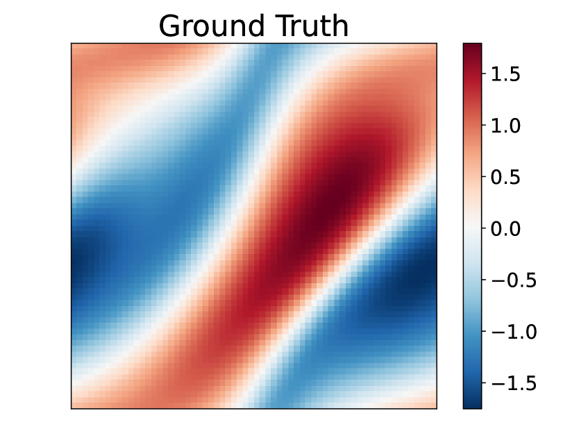
(b)

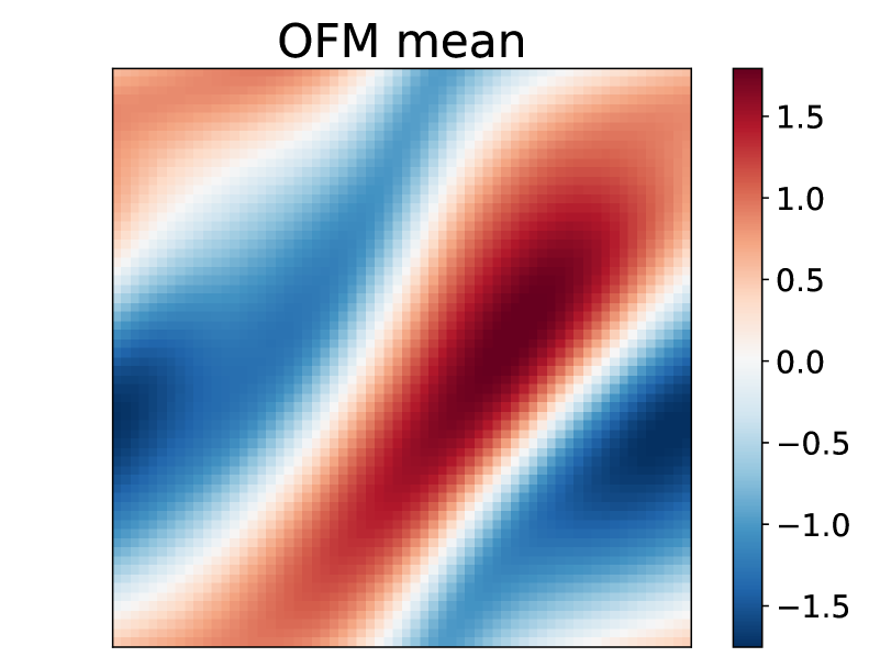
(c)

(d)

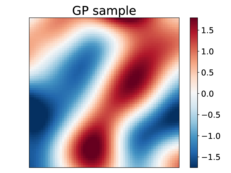
(e)

Figure 6: OFM regression on Navier-Stokes functional data with resolution $64\times 64$. (a) 32 random observations. (b) Ground truth sample (c) Predicted mean from OFM. (d) One posterior sample from OFM. (e) One posterior sample from best fitted GP.

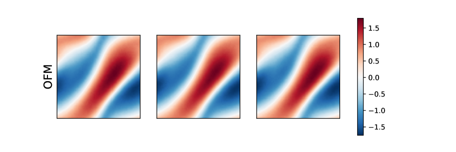
(a)

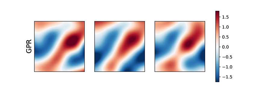
(b)

Figure 8: OFM regression on NS data. (a) Posterior samples from OFM. (b) Posterior samples from GP regression.

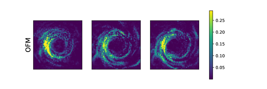
(a)

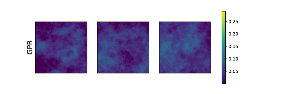
(b)

Figure 9: OFM regression on black hole data. (a) Posterior samples from OFM. (b) Posterior samples from GP regression.

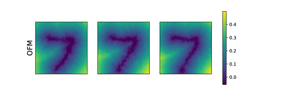
(a)

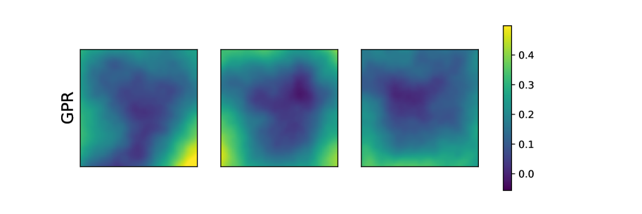
(b)

Figure 10: OFM regression on MNIST-SDF data. (a) Posterior samples from OFM. (b) Posterior samples from GP regression.

A.7 Co-domain functional regression with OFM

In this section, we expand our regression framework to accommodate co-domain settings, as many function datasets feature a co-domain dimension greater than one. For example, earthquake waveform data commonly include three directional components, leading to a three-dimensional co-domain. Similarly, the velocity field in fluid dynamics usually features three directional components, also resulting in a dimension of co-domain of three.

We illustrate this extension through a 2D GP example with a co-domain of 3 (channel dimension of 3). In learning the prior, we define the reference measure ($\nu_{0}$) as a joint measure (Wiener measure) of three identical but independent Gaussian measures while the target measure ($\nu_{1}$) is another Wiener measure. We keep all other parameters unchanged as those described in the 2D GP regression tasks, with the only modification being an increase in the channel dimension from one to three. After training the prior (training detail provided in Appendix A.9), and provided 32 random observations across the three channels at co-locations, we then perform regression with OFM across these channels jointly. As demonstrated in Fig 11, OFM accurately estimate the mean and uncertainty across three channels.

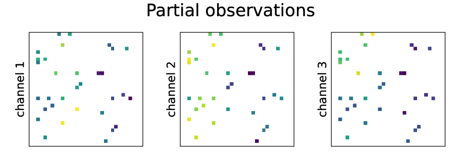
(a)

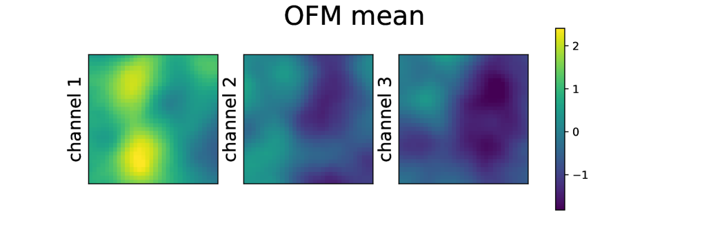
(b)

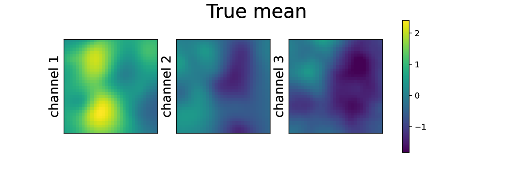
(c)

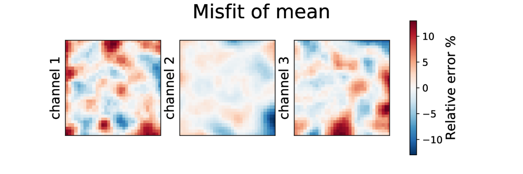
(d)

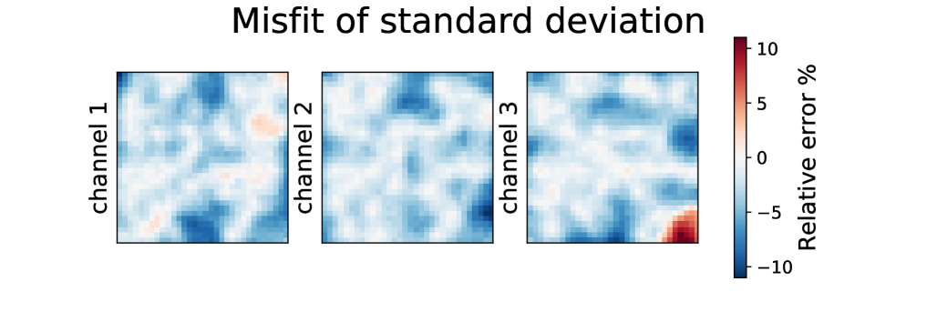
(e)

Figure 11: OFM regression on co-domain GP data with resolution 32x32. (a) 32 random observations at co-locations. (b) Predicted mean from OFM. (c) Ground truth mean from GP regression. (d) Misfit of the predicted mean. (e) Misfit of predicted standard deviation.

A.8 Posterior sampling with Stochastic Gradient Langevin Dynamics

In this section, we describe how to sample from posterior distribution with SGLD. We denote logarithmic posterior distribution (Eq. 27) as $\log\mathbb{P}_{\theta}$ and denote a set of posterior samples as $\{u_{\theta}^{t}\}^{N}_{t=1}$, where each $u_{\theta}^{t}$ is defined on a collection of point $\{x_{i}\}_{i=1}^{m}$.

By following the standard SGLD pipeline as described by Welling & Teh (2011), we can obtain a set of $N$ posterior samples $\{u_{\theta}^{t}\}_{t=1}^{N}$. However, SGLD is known to be sensitive to the choice of regression parameters and can become trapped in local minima, leading to convergence issues, especially in regions of high curvature (Li et al., 2015). To mitigate these challenges, Shi et al. (2024a) proposed that within an invertible framework, drawing a posterior sample $u_{\theta}^{t}$ is equivalent to drawing a sample $a_{\theta}^{t}$ in Gaussian space, since $u_{\theta}^{t}$ uniquely defines $a_{\theta}^{t}$ and vice versa. This approach can stabilize the posterior sampling process and is less sensitive to the regression parameters due to the inherent smoothness of the Gaussian process. Additionally,  Shi et al. (2024a) suggests starting from maximum a posteriori (MAP) estimate of $a_{\theta}^{t}$, denoted as $\overline{a_{\theta}}$, which can reduces the number of burn-in terations needed in SGLD. We adopt the same sampling strategy and refer readers to the detailed discussion in Shi et al. (2024a). The algorithm is reported in Algorithm 1

When the size of observations or context points ($\{\widehat{u}(x_{i})\}_{i=1}^{n}$) is 0, sampling from the posterior degrades to sampling from the prior, the results of which are presented in the subsequent section.

Algorithm 1 Posterior sampling with SGLD

1:Input and Parameters: Logarithmic posterior distribution $\log\mathbb{P}_{\theta}$, temperature $T$, learning rate $\eta_{t}$, MAP $\overline{a}_{\theta}$, burn-in iteration $b$, sampling iteration $t_{N}$, total iteration $N$.

2:Initialization: $a_{\theta}^{0}=\overline{a}_{\theta}$

3:for $t=0,1,2,\ldots,N$ do

4:  Compute gradient of the posterior: $\nabla_{a_{\theta}}\log\mathbb{P}_{\theta}$

5:  Update $a_{\theta}^{t+1}$: $a_{\theta}^{t+1}=a_{\theta}^{t}+\frac{\eta_{t}}{2}\nabla\log\mathbb{P}_{\theta}+\sqrt{\eta_{t}T}\mathcal{N}(0,I)$

6:  if $t\geq b$ then

7:   Every $t_{N}$ iterations: obtain new sample $a_{\theta}^{t+1}$, and corresponding $u_{\theta}^{t+1}$

8:  end if

9:end for

A.9 Prior learning with OFM

We now elaborate on the prior learning process and the corresponding performance evaluation. As shown in Algorithm 2, the training dataset is sampled from the unknown data measure $\nu_{1}$. Concretely, the training dataset consists of $M$ discretized functions $\{u_{i}|D_{i}\}_{i=1}^{M}$, where $u_{i}|D_{i}$ denotes a discretized observation of the $u_{i}$ function.

In practice, to simplify dataset preparation, one often uses the same discretization grid $D_{i}$ for all function samples, e.g. $D_{i}=\{x_{1},\cdots,x_{n}\}$ regardless of the sample index "i". For the consistency of notions, let $h_{0}$ represents a batch of i.i.d discretized functions sampled from the training dataset (equivalently, sampled from $\nu_{1}$). Next, the reference Gaussian process $\nu_{0}=\mathcal{N}(m_{0},C_{0})$ is known and determined by the user. With a slight abuse of notation, We choose to use notation $h_{0},h_{1}$ for consistency purpose, in other parts of this paper, $h_{0},h_{1}$ is replaced with $a,u$ respectively.

For specific experiments setting, we employ Matern kernel to construct the reference GP and to prepare training datasets for 1D GP, 2D GP, and 1D TGP. We have set the kernel length $l=0.01$ with a smoothness factor $\zeta=0.5$ for all reference GPs. OFM maps the GP samples from reference GPs to data samples and is resolution-invariant, which means OFM can be trained with functions at any resolution and evaluated at any resolution.

Algorithm 2 Learning a prior

Input: Reference Gaussian process $\nu_{0}=\mathcal{N}(m_{0},C_{0})$, data measure $\nu_{1}$, batch size $b$, small constant $\sigma_{\text{min}}$, discretized domain $D=\{x_{1},\cdots x_{n}\}$

1:while Training do

2:  $h_{0}\sim\nu_{0};\quad h_{1}\sim\nu_{1}$       # sample functions of size $b$ i.i.d from the measures on $D$

3:  $\pi\leftarrow\mathrm{OT}(h_{0},h_{1})$           # mini-batch optimal transport plan

4:  $(h_{0},h_{1})\sim\pi$

5:  $t\sim\mathcal{U}(0,1)$

6:  $\mu_{t}\leftarrow t\,h_{1}+(1-t)\,h_{0}$

7:  $h_{t}\sim\mathcal{N}(\mu_{t},\sigma_{\text{min}}^{2}C_{0})$

8:  $\mathcal{L}^{\dagger}_{\mathrm{CFM}}(\theta)\leftarrow\bigl{\|}\mathcal{G}_{\theta}(t,x)-(h_{1}-h_{0})\bigr{\|}^{2}$

9:  $\theta\leftarrow\mathrm{Update}\bigl{(}\theta,\nabla_{\theta}\,\mathcal{L}^{\dagger}_{\mathrm{CFM}}(\theta)\bigr{)}$

10:end while

11:return $\mathcal{G}_{\theta}$

1D GP dataset. We choose $l=0.3$ and $\zeta=1.5$ and generate $20,000$ training samples on domain $[0,1]$ with a fixed resolution of 256. We use autocovariance and histogram of point-wise value as metrics for evaluation. We evaluate OFM at several different resolutions shown Fig 12, 13, 14, which demonstrate OFM’s excellent capability to learn the function prior.

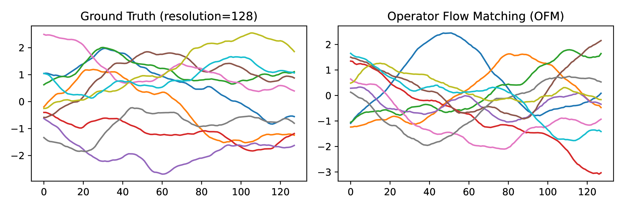
(a)

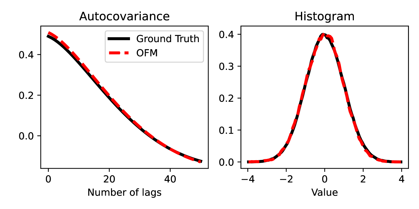
(b)

Figure 12: OFM for 1D GP prior learning, evaluated at resolution=128. (a) Random samples from ground truth and generated by OFM. (b) Autocovariance and histogram comparison

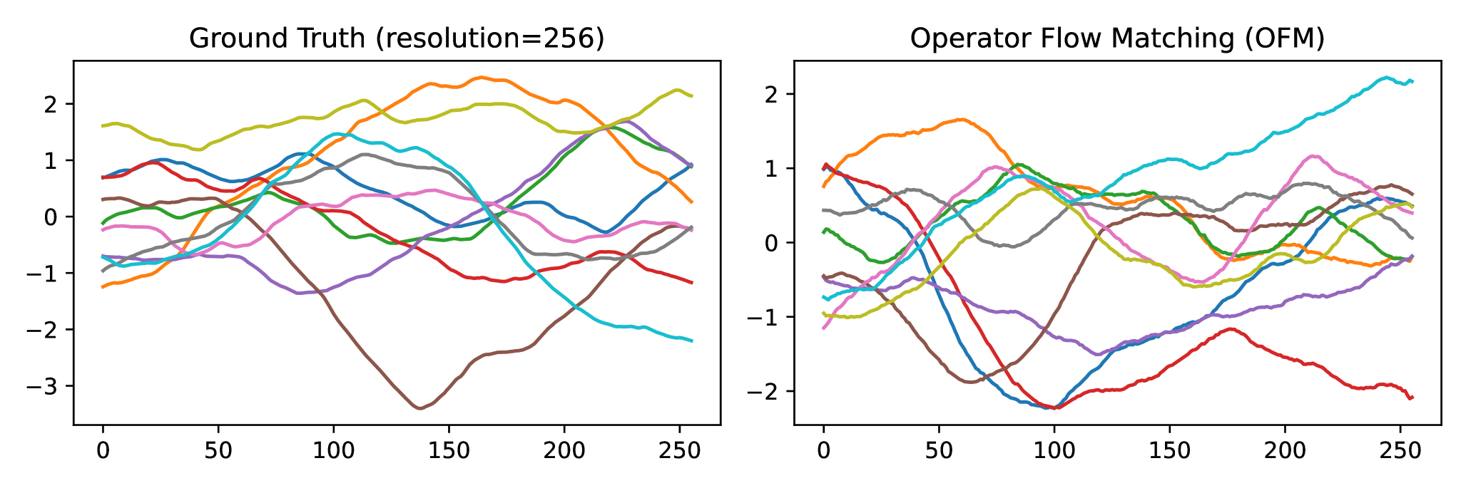
(a)

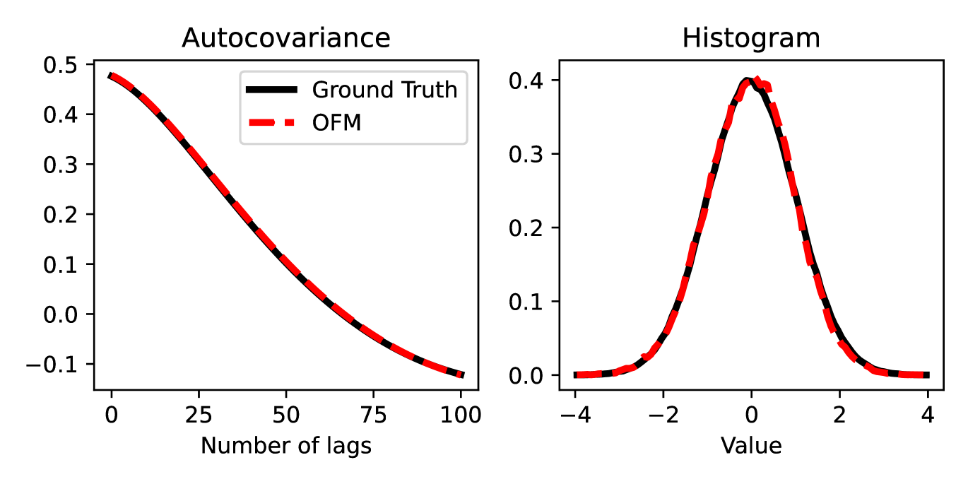
(b)

Figure 13: OFM for 1D GP prior learning, evaluated at resolution=256. (a) Random samples from ground truth and generated by OFM. (b) Autocovariance and histogram comparison

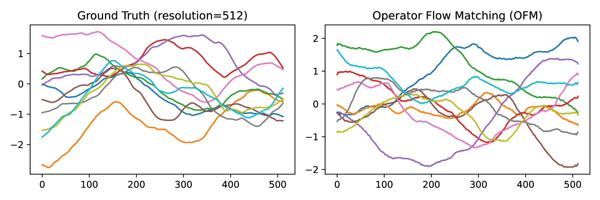
(a)

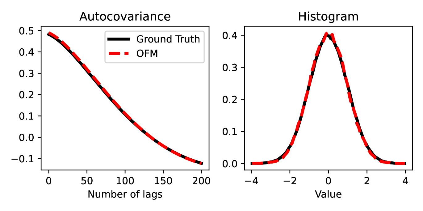
(b)

Figure 14: OFM for 1D GP prior learning, evaluated at resolution=512. (a) Random samples from ground truth and generated by OFM. (b) Autocovariance and histogram comparison

1D TGP dataset. We choose $l=0.3$ and $\zeta=1.5$ and generating $20,000$ training samples on domain $[0,1]$ with a fixed resolution of 256. We set $[-1.2,1.2]$ for the bounds. Results provided in Fig 15, 16, 17.

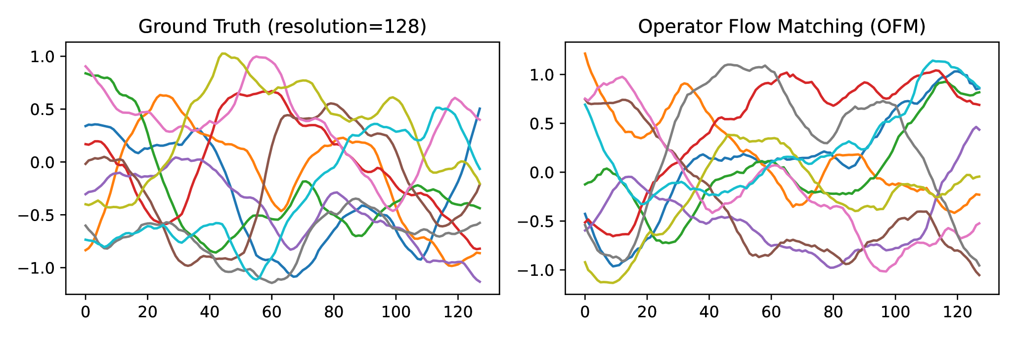
(a)

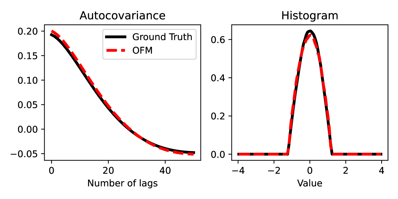
(b)

Figure 15: OFM for 1D TGP prior learning, evaluated at resolution=128. (a) Random samples from ground truth and generated by OFM. (b) Autocovariance and histogram comparison

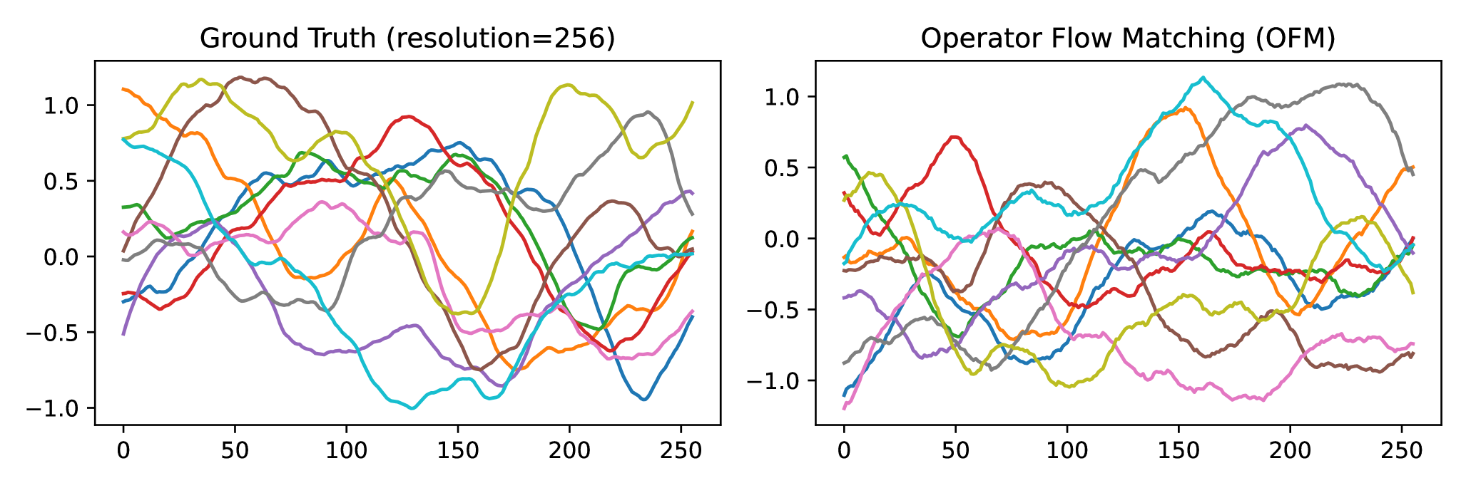
(a)

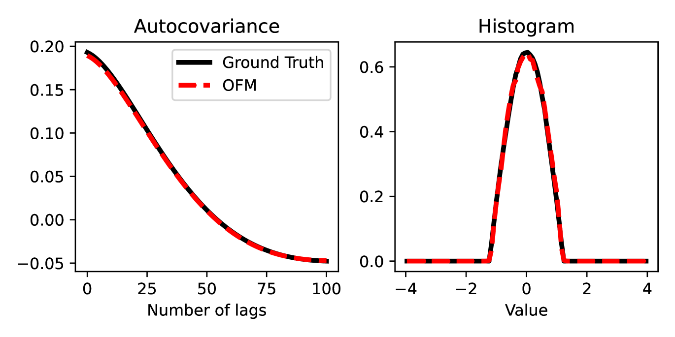
(b)

Figure 16: OFM for 1D TGP prior learning, evaluated at resolution=256. (a) Random samples from ground truth and generated by OFM. (b) Autocovariance and histogram comparison

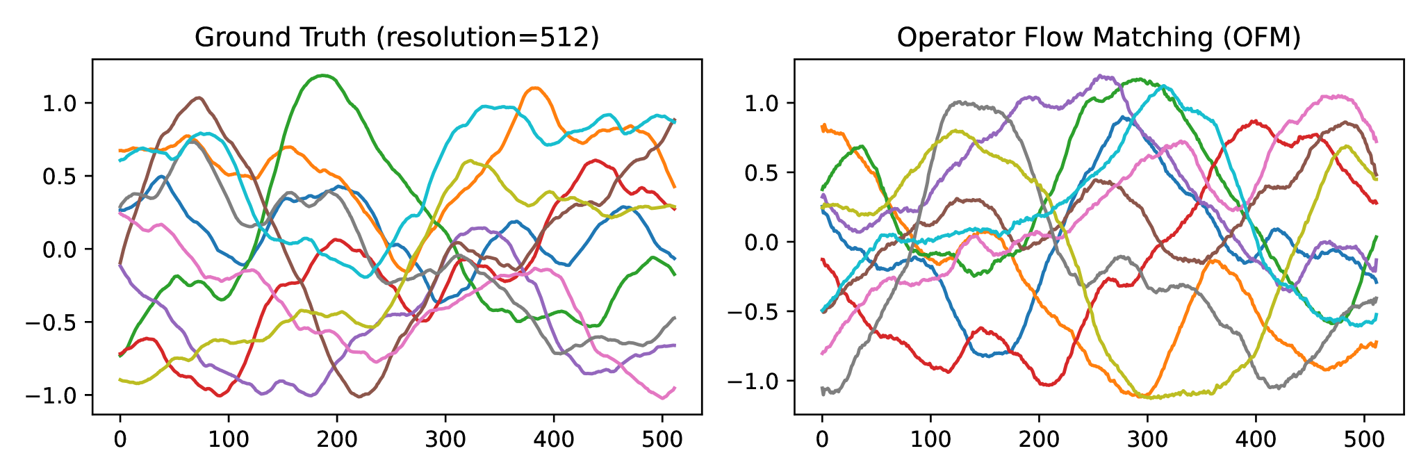
(a)

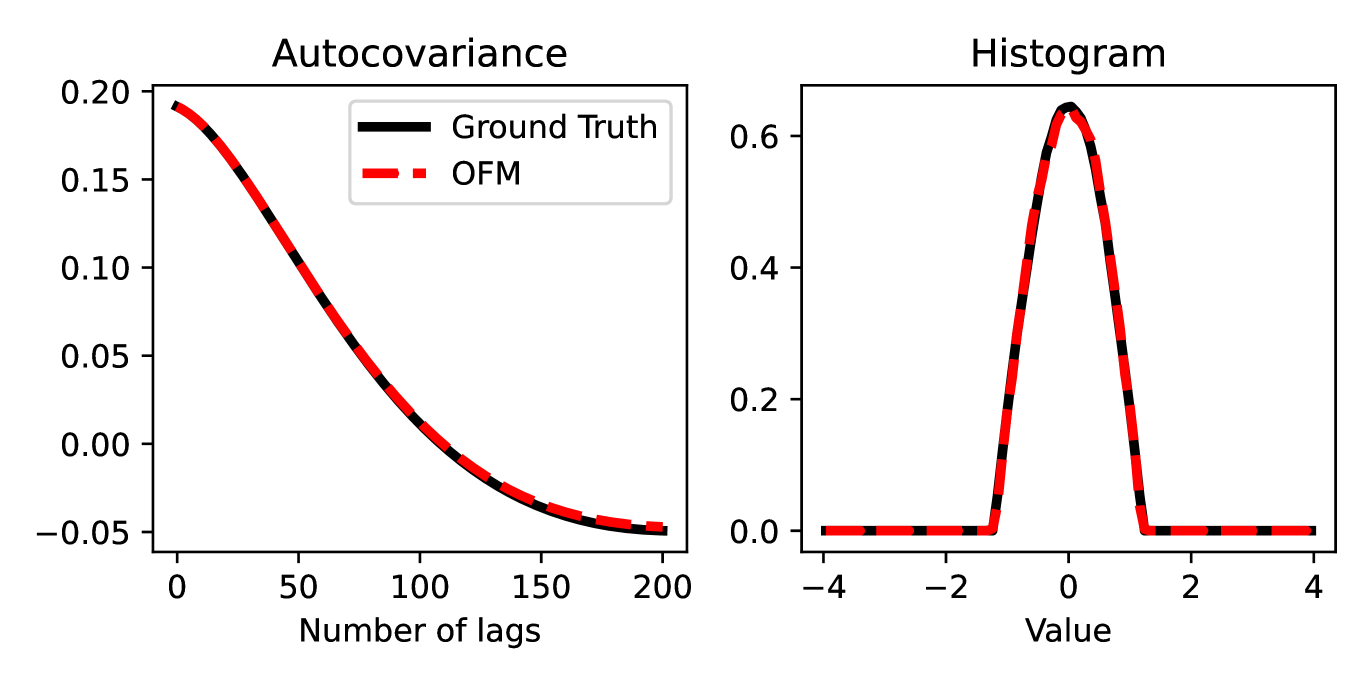
(b)

Figure 17: OFM for 1D TGP prior learning, evaluated at resolution=512. (a) Random samples from ground truth and generated by OFM. (b) Autocovariance and histogram comparison

2D Naiver-Stokes, Black hole, MNIST-SDF datasets. All the following 2D datasets are defined on domain $[0,1]\times[0,1]$ and have a resolution of $64\times 64$. We collected a 2D Navier-Stokes dataset consisting of 20000 samples, with viscosity $=1e-4$ . The results, including zero-shot super-resolution, are provided in Fig 18,  19. The learning of Black hole dataset, generated using expensive Monte Carlo method, is detailed in Fig 20, 21. Additionally, we trained OFM on $20,000$ MNIST-SDF samples, the outcomes are illustrated in Fig 22, 23.

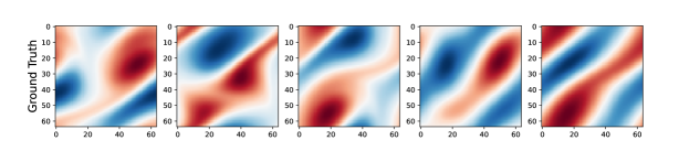
(a)

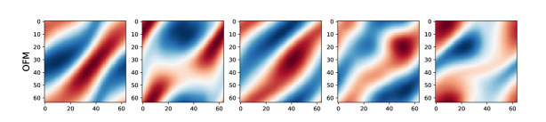
(b)

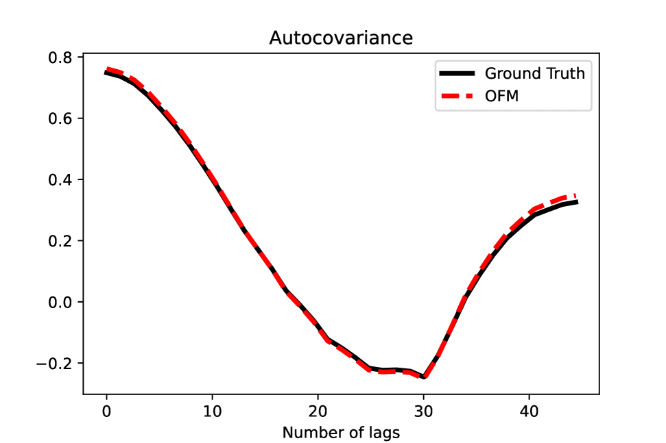
(c)

Figure 18: OFM for 2D N-S prior learning, evaluated at resolution=$64\times 64$. (a) Random samples from ground truth. (b) Random samples generated by OFM. (c) Autocovariance comparison

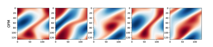
(a)

Figure 19: OFM for 2D N-S prior learning, evaluated at $128\times 128$ resolution (zero-shot super-resolution)

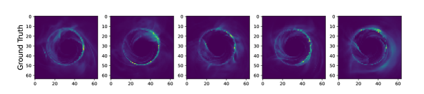
(a)

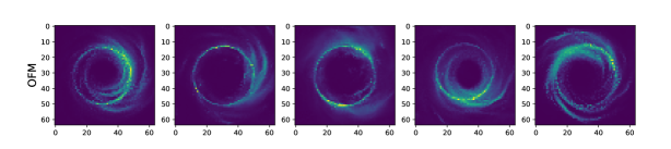
(b)

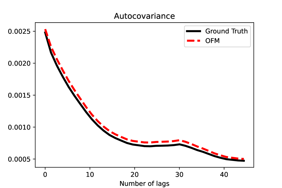
(c)

Figure 20: OFM for 2D black hole prior learning, evaluated at resolution=64. (a) Random samples from ground truth. (b) Random samples generated by OFM. (c) Autocovariance comparison

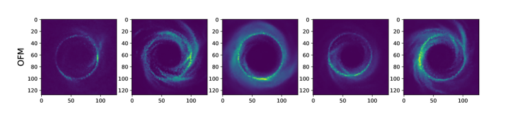
(a)

Figure 21: OFM for 2D black hole prior learning, evaluated at $128\times 128$ resolution (zero-shot super-resolution)

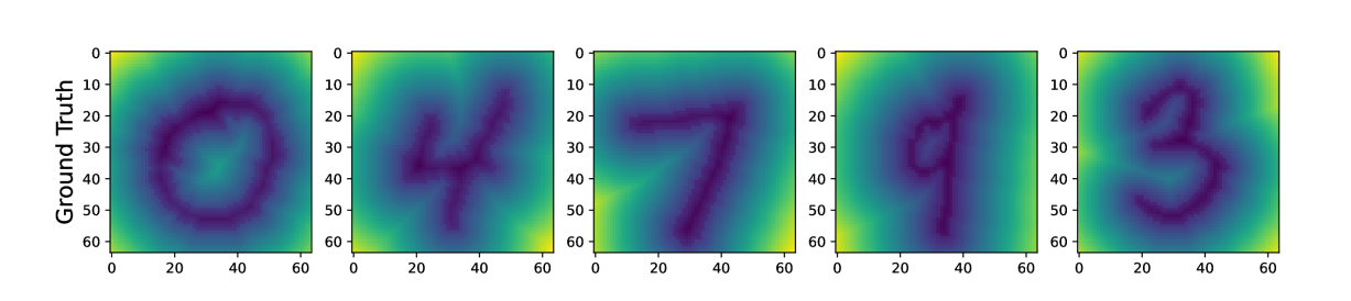
(a)

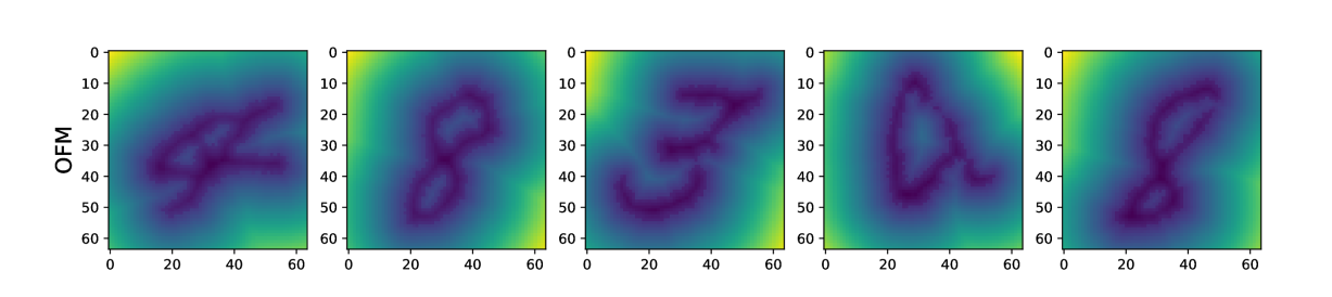
(b)

Figure 22: OFM for 2D MNIST-SDF prior learning, evaluated at $64\times 64$ resolution. (a) Random samples from ground truth. (b) Random samples generated by OFM.

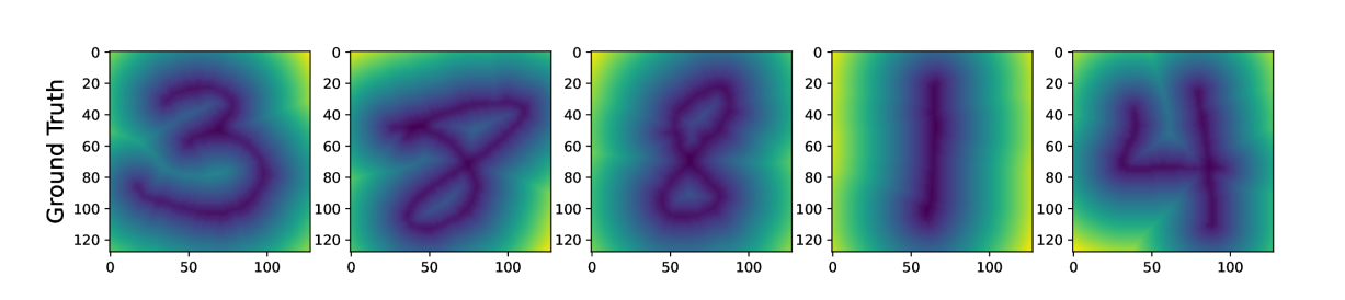
(a)

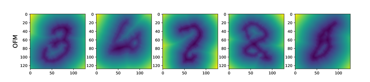
(b)

Figure 23: OFM for 2D MNIST-SDF prior learning, evaluated at $128\times 128$ resolution. (a) Random samples from ground truth. (b) Random samples generated by OFM.

A.10 Details of experimental setup

In this section, we outline the details of experiments setup used in this paper. Since regression with OFM requires learning the prior first, we list the parameters used for learning the prior and regression separately. We employ FNO as the backbone, implemented using neuraloperator library (Li et al., 2021). All time reported in the subsequent tables are based on one computations performed using a single NVIDIA RTX A6000 (48 GB) graphics card.

Table 2 details the parameters used for training the prior. For instance, in the 1D GP prior learning experiment, the dataset consists of 20,000 samples, each with a co-domain dimension (or channel) of one. The batch size is set at 1024, and the model is trained over 500 epochs. The total training time is about 0.76 hours, and the size of the trained model is 37.1 megabytes.

Tables 3, 4, and 5 detail the parameters for SGLD sampling as described in Algorithm 1. For example, in the 1D GP regression as an example, the regression takes 40,000 iterations with a burn-in phase of 3,000 iterations. Posterior samples are collected every 10 iterations. The temperature for the injected noise during the gradient update is set at 1, and the learning rate decays exponentially from 0.005 to 0.004 (defined in Algorithm 1). We average 32 runs with the Hutchinson trace estimator to evaluate the likelihood, utilizing GPU parallel computing. The noise level, as specified in Equation 27, is 0.01 in this regression task. Then given 6 random observations, we ask for the posterior samples across 128 points. The GPU memory usage for the regression task is 4 gigabytes, with the total runtime to 4.91 hours.

Datasets	Size of Dataset	Channels	Batch Size	Epochs	Training Time	Model Size
1D GP	$2\cdot 10^{4}$	1	1024	$5\cdot 10^{2}$	$0.76$ h	37.1 MB
1D TGP	$2\cdot 10^{4}$	1	1024	$5\cdot 10^{2}$	1.24 h	37.1 MB
2D GP	$2\cdot 10^{4}$	1	256	$5\cdot 10^{2}$	1.14 h	76 MB
2D co-domain GP	$2\cdot 10^{4}$	3	256	$5\cdot 10^{2}$	1.01 h	76 MB
2D N-S	$2\cdot 10^{4}$	1	256	$5\cdot 10^{2}$	3.79 h	286 MB
2D Black hole	$1.2\cdot 10^{4}$	1	256	$5\cdot 10^{2}$	2.28 h	286 MB
2D MNIST-SDF	$2\cdot 10^{4}$	1	256	$5\cdot 10^{2}$	8.31 h	286 MB

Table 2: Parameters used in experiments of prior learning

Datasets	Total Iteration	Burn-in Iteration	Sampling Iterations	Temperature of Noise
1D GP	$4\cdot 10^{4}$	$3\cdot 10^{3}$	10	1
1D TGP	$4\cdot 10^{4}$	$3\cdot 10^{3}$	10	1
2D GP	$2\cdot 10^{4}$	$3\cdot 10^{3}$	10	1
2D co-domain GP	$2\cdot 10^{4}$	$3\cdot 10^{3}$	10	1
2D N-S	$2\cdot 10^{4}$	$3\cdot 10^{3}$	10	1
2D Black hole	$2\cdot 10^{4}$	$3\cdot 10^{3}$	10	1
2D MNIST-SDF	$2\cdot 10^{4}$	$3\cdot 10^{3}$	10	1

Table 3: Parameters used in regression experiments - Part A

Datasets	Initial Learning Rate	End Learning Rate	Hutchinson Samples	Noise Level
1D GP	$5\cdot 10^{-3}$	$4\cdot 10^{-3}$	32	$1\cdot 10^{-2}$
1D TGP	$5\cdot 10^{-3}$	$4\cdot 10^{-3}$	32	$1\cdot 10^{-3}$
2D GP	$1\cdot 10^{-3}$	$8\cdot 10^{-4}$	32	$1\cdot 10^{-2}$
2D co-domain GP	$1\cdot 10^{-3}$	$8\cdot 10^{-4}$	16	$1\cdot 10^{-2}$
2D N-S	$3\cdot 10^{-3}$	$2\cdot 10^{-3}$	8	$1\cdot 10^{-3}$
2D Black hole	$5\cdot 10^{-3}$	$4\cdot 10^{-3}$	8	$1\cdot 10^{-3}$
2D MNIST-SDF	$5\cdot 10^{-3}$	$4\cdot 10^{-3}$	8	$1\cdot 10^{-3}$

Table 4: Parameters used in regression experiments - Part B

Datasets	Number of Observations	Inquired Grids	GPU Memory	Running Time
1D GP	6	128	4 GB	4.91 h
1D TGP	3	128	4 GB	5.42 h
2D GP	32	$32\times 32$	22 GB	9.70 h
2D co-domain GP	32	$32\times 32$	31 GB	5.05 h
2D N-S	32	$64\times 64$	44 GB	13.65 h
2D Black hole	32	$64\times 64$	44 GB	13.37 h
2D MNIST-SDF	64	$64\times 64$	44 GB	9.41 h

Table 5: Parameters used in regression experiment - Part C

A.11 Detailed analysis of OFM and comparison with existing methods

In this section, we elaborate the connection and difference with pervious work, highlight contributions and potential limitations of our work. The regression with OFM involves a two-steps process: (i) learning a prior on function space, and (ii) sampling from the posterior given observations. Consequently, the OFM framework has connections with both generative models on function space and the models developed for functional regression. In the following, we provide a comprehensive comparative analysis with related models and baselines, including operator flow (OpFlow) (Shi et al., 2024a), conditional optimal transport flow matching (COT-FM) (Kerrigan et al., 2024), neural processes (NPs) (Garnelo et al., 2018; Dutordoir et al., 2023)

Comparison with OpFlow. OpFlow introduces invertible neural operators, which generalizes RealNVP (Dinh et al., 2017) to function space and maps any collection of points sampled from a GP to a new collection of points in the data space, using the maximum likelihood principle (Shi et al., 2024a). This method captures the likelihood of any collection of point consistently as the resolution increases and allows for UFR using SGLD. Despite these advantages, the requirement for an invertible neural operator brings training and expressiveness challenges. On the contrary, OFM adopts a simulation-free ODE framework for prior learning, which offers enhanced expressiveness and ensures training stability through a simple regression objective while avoiding using the invertible neural operator. In addition, OFM proposes a non-trivial extension of UFR to the simulation-free ODE framework. These improvements render OFM a more practical solution for challenging functional regression tasks.

Comparison with COT-FM. COT-FM (Kerrigan et al., 2024) proposes a conditional generalization of Benamou-Brenier Theorem (Benamou & Brenier, 2000), formulating a conditional optimal transport plan that applicable for both Euclidean and Hilbert space. In contrast, OFM employs an unconditional optimal transport plan in Hilbert space based on dynamic Kantorovich formulation, which is initially generalized for unbalanced optimal transport (Chizat et al., 2018). The advantage of COT-FM lies in its ability to flexibly incorporate specific conditions tailored for conditional generative tasks. However, COT-FM is not suitable for functional regression tasks due to: (i) COT-FM is contingent upon both the reference and target being influenced by conditions, and the vector field learnt is triangular, designed to transport jointly the coupling of a reference measure and a condition measure. In UFR setting, the learnt prior is required to be unconditioned, (ii) the coupling with condition measure typically prevents inducing valid stochastic process, even when the reference measure is a Gaussian measure, (iii) cannot provide point evaluation of probability density. Last, We should notice, the development of OFM is different and independent of COT-FM, the former with a focus on stochastic process learning and Bayesian functional regression.

Comparison with NPs. NPs were developed to address the computational and restrictive prior challenges of Gaussian Processes, utilizing neural networks for efficiency  (Garnelo et al., 2018). However, several recent studies have discussed the drawbacks in the formulation of NPs, raising concerns that NPs might not learn the underlying function distribution (Rahman et al., 2022; Dupont et al., 2022; Shi et al., 2024a).

Notably, NPs treats the point cloud data as a set of values, ignoring the metric space of the data (Dupont et al., 2022). This can lead to misinterpretations of a function sampled at different resolutions as distinct functions (Appendix A.1 of (Rahman et al., 2022)). Furthermore, NPs rely on encoding input data into finite-dimensional, Gaussian-distributed latent variables before projecting these into an infinite-dimensional space. This process tends to lose consistency at higher resolutions. Moreover, the Bayesian regression framework underpinning NPs focuses on point sets rather than the functions themselves, leading to a dilution of prior information with increasing data points.

In recent study, diffusion-based variants of NPs (NDP) (Dutordoir et al., 2023), was proposed to leverage the expressiveness of diffusion models (Ho et al., 2020; Song et al., 2021). Nonetheless, the formulation of NDP does not address the aforementioned issues of NPs and introduces two more problems: (i) NDP fails to induce a valid stochastic process as it does not satisfy the marginal consistency criterion required by Kolmogorov Extension Theorem (Kolmogorov & Bharucha-Reid, 2018), and (ii) it relies on uncorrelated Gaussian noise for denoising, which is not applicable in function spaces (Lim et al., 2023). Oppositely, OFM establishes a more theoretically sound framework by rigorously defining learning within function spaces. Additionally, Bayesian functional regression within the OFM framework adheres to valid stochastic processes, offering a robust and theoretically grounded solution.

Contribution and Limitations. In conclusion, OFM represents the first simulation-free continuous normalizing flow (ODE framework) designed for functional regression purpose, demonstrating superior performance over existing baselines. The theory development for generalizing flow matching to stochastic process as well as development of optimal-transport infinite-dimensional flow matching are considered as additional contributions.

Despite these advances, the current regression framework with OFM is primarily limited to low-dimensional data (1D and 2D in this study). This limitation stems from the challenges associated with learning operators for functions defined on high-dimensional domains—an area that remains underdeveloped both computationally and in terms of dataset availability (Kovachki et al., 2023). Additionally, while the time complexity for regression with OFM is $\mathcal{O}(D^{2})$, the incorporation of additional components significantly increases its computational resource requirements compared to classical GP regression.

References

- Ambrosio et al. (2008) Luigi Ambrosio, Nicola Gigli, and Giuseppe Savaré. Gradient flows: in metric spaces and in the space of probability measures. Springer Science & Business Media, 2008. ISBN 3-7643-8722-X.
- Azizzadenesheli et al. (2024) Kamyar Azizzadenesheli, Nikola Kovachki, Zongyi Li, Miguel Liu-Schiaffini, Jean Kossaifi, and Anima Anandkumar. Neural operators for accelerating scientific simulations and design. Nature Reviews Physics, 6(5):320–328, May 2024. ISSN 2522-5820. doi: 10.1038/s42254-024-00712-5. URL https://www.nature.com/articles/s42254-024-00712-5. Publisher: Nature Publishing Group.
- Benamou & Brenier (2000) Jean-David Benamou and Yann Brenier. A computational fluid mechanics solution to the Monge-Kantorovich mass transfer problem. Numerische Mathematik, 84(3):375–393, 2000. URL https://www.iap.fr/actualites/laune/2022/TransportOptimal/ark%20_67375_VQC-XB4DR0Z3-2.pdf. Publisher: Springer-Verlag Berlin/Heidelberg.
- Bogachev (1998) Vladimir Igorevich Bogachev. Gaussian measures. American Mathematical Soc., 1998. ISBN 0-8218-1054-5. Issue: 62.
- Brémaud (2020) Pierre Brémaud. Probability Theory and Stochastic Processes. Universitext. Springer International Publishing, Cham, 2020. ISBN 978-3-030-40182-5 978-3-030-40183-2. doi: 10.1007/978-3-030-40183-2. URL http://link.springer.com/10.1007/978-3-030-40183-2.
- Chen et al. (2019) Ricky T. Q. Chen, Yulia Rubanova, Jesse Bettencourt, and David Duvenaud. Neural Ordinary Differential Equations, December 2019. URL http://arxiv.org/abs/1806.07366. arXiv:1806.07366 [cs, stat].
- Chizat et al. (2018) Lénaïc Chizat, Gabriel Peyré, Bernhard Schmitzer, and François-Xavier Vialard. Unbalanced optimal transport: Dynamic and Kantorovich formulations. Journal of Functional Analysis, 274(11):3090–3123, June 2018. ISSN 0022-1236. doi: 10.1016/j.jfa.2018.03.008. URL https://www.sciencedirect.com/science/article/pii/S0022123618301058.
- Damianou & Lawrence (2013) Andreas Damianou and Neil D Lawrence. Deep gaussian processes. pp. 207–215. PMLR, 2013.
- Dinh et al. (2017) Laurent Dinh, Jascha Sohl-Dickstein, and Samy Bengio. Density estimation using Real NVP, February 2017. URL http://arxiv.org/abs/1605.08803. arXiv:1605.08803.
- Dupont et al. (2022) Emilien Dupont, Yee Whye Teh, and Arnaud Doucet. Generative Models as Distributions of Functions, February 2022. URL http://arxiv.org/abs/2102.04776. arXiv:2102.04776.
- Dutordoir et al. (2023) Vincent Dutordoir, Alan Saul, Zoubin Ghahramani, and Fergus Simpson. Neural Diffusion Processes, June 2023. URL http://arxiv.org/abs/2206.03992. arXiv:2206.03992 [cs, stat].
- Fjelde et al. (2024) Tor Fjelde, Émile Mathieu, and Vincent Dutordoir. An introduction to Flow Matching · Cambridge MLG Blog, January 2024. URL https://mlg.eng.cam.ac.uk/blog/2024/01/20/flow-matching.html#mjx-eqn%3Aeq%3Acf-from-cond-vf.
- Garnelo et al. (2018) Marta Garnelo, Jonathan Schwarz, Dan Rosenbaum, Fabio Viola, Danilo J. Rezende, S. M. Ali Eslami, and Yee Whye Teh. Neural Processes, July 2018. URL http://arxiv.org/abs/1807.01622. arXiv:1807.01622 [cs, stat].
- Grathwohl et al. (2018) Will Grathwohl, Ricky T. Q. Chen, Jesse Bettencourt, Ilya Sutskever, and David Duvenaud. FFJORD: Free-form Continuous Dynamics for Scalable Reversible Generative Models, October 2018. URL http://arxiv.org/abs/1810.01367. arXiv:1810.01367 [cs, stat].
- Ho et al. (2020) Jonathan Ho, Ajay Jain, and Pieter Abbeel. Denoising Diffusion Probabilistic Models, December 2020. URL http://arxiv.org/abs/2006.11239. arXiv:2006.11239 [cs, stat].
- Hutchinson (1989) Michael F Hutchinson. A stochastic estimator of the trace of the influence matrix for Laplacian smoothing splines. Communications in Statistics-Simulation and Computation, 18(3):1059–1076, 1989. ISSN 0361-0918. Publisher: Taylor & Francis.
- Jankowiak et al. (2020) Martin Jankowiak, Geoff Pleiss, and Jacob R. Gardner. Deep Sigma Point Processes, December 2020. URL http://arxiv.org/abs/2002.09112. arXiv:2002.09112 [cs, stat].
- Kantorovich & Rubinshtein (1958) Leonid Vasilevich Kantorovich and SG Rubinshtein. On a space of totally additive functions. Vestnik of the St. Petersburg University: Mathematics, 13(7):52–59, 1958. ISSN 1063-4541. Publisher: Allerton Press, Inc.
- Kerrigan et al. (2023a) Gavin Kerrigan, Justin Ley, and Padhraic Smyth. Diffusion Generative Models in Infinite Dimensions, February 2023a. URL http://arxiv.org/abs/2212.00886. arXiv:2212.00886 [cs, stat].
- Kerrigan et al. (2023b) Gavin Kerrigan, Giosue Migliorini, and Padhraic Smyth. Functional Flow Matching, December 2023b. URL http://arxiv.org/abs/2305.17209. arXiv:2305.17209 [cs, stat].
- Kerrigan et al. (2024) Gavin Kerrigan, Giosue Migliorini, and Padhraic Smyth. Dynamic Conditional Optimal Transport through Simulation-Free Flows, May 2024. URL http://arxiv.org/abs/2404.04240. arXiv:2404.04240.
- Kim et al. (2019) Hyunjik Kim, Andriy Mnih, Jonathan Schwarz, Marta Garnelo, Ali Eslami, Dan Rosenbaum, Oriol Vinyals, and Yee Whye Teh. Attentive Neural Processes, July 2019. URL http://arxiv.org/abs/1901.05761. arXiv:1901.05761 [cs, stat].
- Kolmogorov & Bharucha-Reid (2018) Andreĭ Nikolaevich Kolmogorov and Albert T Bharucha-Reid. Foundations of the theory of probability: Second English Edition. Courier Dover Publications, 2018. ISBN 0-486-82159-5.
- Kou et al. (2013) Peng Kou, Feng Gao, and Xiaohong Guan. Sparse online warped Gaussian process for wind power probabilistic forecasting. Applied energy, 108:410–428, 2013. ISSN 0306-2619. Publisher: Elsevier.
- Kovachki et al. (2023) Nikola Kovachki, Zongyi Li, Burigede Liu, Kamyar Azizzadenesheli, Kaushik Bhattacharya, Andrew Stuart, and Anima Anandkumar. Neural Operator: Learning Maps Between Function Spaces With Applications to PDEs. Journal of Machine Learning Research, 24(89):1–97, 2023. ISSN 1533-7928. URL http://jmlr.org/papers/v24/21-1524.html.
- Li et al. (2015) Chunyuan Li, Changyou Chen, David Carlson, and Lawrence Carin. Preconditioned Stochastic Gradient Langevin Dynamics for Deep Neural Networks, December 2015. URL http://arxiv.org/abs/1512.07666. arXiv:1512.07666.
- Li et al. (2021) Zongyi Li, Nikola Kovachki, Kamyar Azizzadenesheli, Burigede Liu, Kaushik Bhattacharya, Andrew Stuart, and Anima Anandkumar. Fourier Neural Operator for Parametric Partial Differential Equations, May 2021. URL http://arxiv.org/abs/2010.08895. arXiv:2010.08895 [cs, math].
- Li et al. (2023) Zongyi Li, Nikola Borislavov Kovachki, Chris Choy, Boyi Li, Jean Kossaifi, Shourya Prakash Otta, Mohammad Amin Nabian, Maximilian Stadler, Christian Hundt, Kamyar Azizzadenesheli, and Anima Anandkumar. Geometry-Informed Neural Operator for Large-Scale 3D PDEs, September 2023. URL http://arxiv.org/abs/2309.00583. arXiv:2309.00583.
- Lim et al. (2023) Jae Hyun Lim, Nikola B. Kovachki, Ricardo Baptista, Christopher Beckham, Kamyar Azizzadenesheli, Jean Kossaifi, Vikram Voleti, Jiaming Song, Karsten Kreis, Jan Kautz, Christopher Pal, Arash Vahdat, and Anima Anandkumar. Score-based Diffusion Models in Function Space, November 2023. URL http://arxiv.org/abs/2302.07400. arXiv:2302.07400 [cs, math, stat].
- Lipman et al. (2023) Yaron Lipman, Ricky T. Q. Chen, Heli Ben-Hamu, Maximilian Nickel, and Matt Le. Flow Matching for Generative Modeling, February 2023. URL http://arxiv.org/abs/2210.02747. arXiv:2210.02747 [cs, stat].
- Liu et al. (2020) Haitao Liu, Yew-Soon Ong, Xiaobo Shen, and Jianfei Cai. When Gaussian process meets big data: A review of scalable GPs. IEEE transactions on neural networks and learning systems, 31(11):4405–4423, 2020. ISSN 2162-237X. Publisher: IEEE.
- Maroñas et al. (2021) Juan Maroñas, Oliver Hamelijnck, Jeremias Knoblauch, and Theodoros Damoulas. Transforming Gaussian processes with normalizing flows. pp. 1081–1089. PMLR, 2021. ISBN 2640-3498.
- Papamakarios et al. (2021) George Papamakarios, Eric Nalisnick, Danilo Jimenez Rezende, Shakir Mohamed, and Balaji Lakshminarayanan. Normalizing flows for probabilistic modeling and inference. Journal of Machine Learning Research, 22(57):1–64, 2021. ISSN 1533-7928.
- Pathak et al. (2022) Jaideep Pathak, Shashank Subramanian, Peter Harrington, Sanjeev Raja, Ashesh Chattopadhyay, Morteza Mardani, Thorsten Kurth, David Hall, Zongyi Li, Kamyar Azizzadenesheli, Pedram Hassanzadeh, Karthik Kashinath, and Animashree Anandkumar. FourCastNet: A Global Data-driven High-resolution Weather Model using Adaptive Fourier Neural Operators, February 2022. URL http://arxiv.org/abs/2202.11214. arXiv:2202.11214.
- Pidstrigach et al. (2023) Jakiw Pidstrigach, Youssef Marzouk, Sebastian Reich, and Sven Wang. Infinite-Dimensional Diffusion Models, October 2023. URL http://arxiv.org/abs/2302.10130. arXiv:2302.10130 [cs, math, stat].
- Rahman et al. (2022) Md Ashiqur Rahman, Manuel A. Florez, Anima Anandkumar, Zachary E. Ross, and Kamyar Azizzadenesheli. Generative Adversarial Neural Operators, October 2022. URL http://arxiv.org/abs/2205.03017. arXiv:2205.03017 [cs, math].
- Salimbeni & Deisenroth (2017) Hugh Salimbeni and Marc Deisenroth. Doubly stochastic variational inference for deep Gaussian processes. Advances in neural information processing systems, 30, 2017.
- Shi et al. (2024a) Yaozhong Shi, Angela F. Gao, Zachary E. Ross, and Kamyar Azizzadenesheli. Universal Functional Regression with Neural Operator Flows, November 2024a. URL http://arxiv.org/abs/2404.02986. arXiv:2404.02986 [cs] version: 3.
- Shi et al. (2024b) Yaozhong Shi, Grigorios Lavrentiadis, Domniki Asimaki, Zachary E. Ross, and Kamyar Azizzadenesheli. Broadband Ground-Motion Synthesis via Generative Adversarial Neural Operators: Development and Validation. Bulletin of the Seismological Society of America, 114(4):2151–2171, August 2024b. ISSN 0037-1106, 1943-3573. doi: 10.1785/0120230207. URL https://pubs.geoscienceworld.org/bssa/article/114/4/2151/636448/Broadband-Ground-Motion-Synthesis-via-Generative.
- Sitzmann et al. (2020) Vincent Sitzmann, Eric Chan, Richard Tucker, Noah Snavely, and Gordon Wetzstein. Metasdf: Meta-learning signed distance functions. Advances in Neural Information Processing Systems, 33:10136–10147, 2020.
- Skilling (1989) John Skilling. The eigenvalues of mega-dimensional matrices. Maximum Entropy and Bayesian Methods: Cambridge, England, 1988, pp. 455–466, 1989. ISSN 9048140447. Publisher: Springer.
- Song et al. (2021) Yang Song, Jascha Sohl-Dickstein, Diederik P. Kingma, Abhishek Kumar, Stefano Ermon, and Ben Poole. Score-Based Generative Modeling through Stochastic Differential Equations, February 2021. URL http://arxiv.org/abs/2011.13456. arXiv:2011.13456 [cs, stat].
- Sun et al. (2023) Hongyu Sun, Zachary E. Ross, Weiqiang Zhu, and Kamyar Azizzadenesheli. Phase Neural Operator for Multi-Station Picking of Seismic Arrivals. Geophysical Research Letters, 50(24):e2023GL106434, 2023. ISSN 1944-8007. doi: 10.1029/2023GL106434. URL https://onlinelibrary.wiley.com/doi/abs/10.1029/2023GL106434. _eprint: https://onlinelibrary.wiley.com/doi/pdf/10.1029/2023GL106434.
- Swiler et al. (2020) Laura P Swiler, Mamikon Gulian, Ari L Frankel, Cosmin Safta, and John D Jakeman. A survey of constrained Gaussian process regression: Approaches and implementation challenges. Journal of Machine Learning for Modeling and Computing, 1(2), 2020. ISSN 2689-3967. Publisher: Begel House Inc.
- Tong et al. (2024) Alexander Tong, Kilian Fatras, Nikolay Malkin, Guillaume Huguet, Yanlei Zhang, Jarrid Rector-Brooks, Guy Wolf, and Yoshua Bengio. Improving and generalizing flow-based generative models with minibatch optimal transport, March 2024. URL http://arxiv.org/abs/2302.00482. arXiv:2302.00482 [cs].
- Villani (2009) Cédric Villani. Optimal Transport, volume 338 of Grundlehren der mathematischen Wissenschaften. Springer, Berlin, Heidelberg, 2009. ISBN 978-3-540-71049-3 978-3-540-71050-9. doi: 10.1007/978-3-540-71050-9. URL http://link.springer.com/10.1007/978-3-540-71050-9.
- Welling & Teh (2011) Max Welling and Yee Whye Teh. Bayesian learning via stochastic gradient langevin dynamics. In Proceedings of the 28th International Conference on International Conference on Machine Learning, ICML’11, pp. 681–688, Madison, WI, USA, June 2011. Omnipress. ISBN 978-1-4503-0619-5.
- Wen et al. (2023) Gege Wen, Zongyi Li, Qirui Long, Kamyar Azizzadenesheli, Anima Anandkumar, and Sally M. Benson. Real-time high-resolution CO2 geological storage prediction using nested Fourier neural operators. Energy & Environmental Science, 16(4):1732–1741, April 2023. ISSN 1754-5706. doi: 10.1039/D2EE04204E. URL https://pubs.rsc.org/en/content/articlelanding/2023/ee/d2ee04204e. Publisher: The Royal Society of Chemistry.
- Williams & Rasmussen (2006) Christopher KI Williams and Carl Edward Rasmussen. Gaussian processes for machine learning, volume 2. MIT press Cambridge, MA, 2006. Issue: 3.
- Yang et al. (2021) Yan Yang, Angela F. Gao, Jorge C. Castellanos, Zachary E. Ross, Kamyar Azizzadenesheli, and Robert W. Clayton. Seismic wave propagation and inversion with Neural Operators, October 2021. URL http://arxiv.org/abs/2108.05421. arXiv:2108.05421.
- Yang et al. (2023) Yan Yang, Angela F. Gao, Kamyar Azizzadenesheli, Robert W. Clayton, and Zachary E. Ross. Rapid Seismic Waveform Modeling and Inversion with Neural Operators, April 2023. URL http://arxiv.org/abs/2209.11955. arXiv:2209.11955.