Pz Cats: Photometric redshift catalogs based on DES Y3 BAO sample

Abstract

The photometric redshift estimation (photo-z) has been developed over the years with various methods. In this work, we analyse four different photo-z estimators using the Dark Energy Survey Y3 BAO Sample: ANNz2, BPZ, ENF, and DNF. Unlike what is usually found in the literature, we investigate the possibility of selecting the best galaxies according to their redshift Probability Distribution Function (PDF). We selected 25,760 galaxies from four different spectroscopic surveys and cross-matched them with the photo-z sample. These galaxies served to understand the redshift bias and its 68th percentile $\sigma_{68}$. We found that within a range of $0.79<z_{p}<0.85$ there is the lowest $\sigma$ for all the estimators we analysed. DNF has the biggest absolute value of the bias ($\sigma$), while ENF, ANNz2 and BPZ lose precision for a redshift range below 0.7 and higher than 0.9. If one wants to pick the best galaxies by removing the bins with the worst bias, one will find that ANNz2 is the most robust algorithm for all chosen criteria. When selecting the best PDFs, the resulting sub-samples gave BPZ with more selected objects. ANNz2 shows better precision, ENF has the worst selection of Gaussian PDFs, with very few galaxies left for an LSS study. We also showed that even though the PDFs are smooth, there are catastrophic redshift results. Lastly, DNF is the worst in precision but with sufficient galaxies for cosmological analysis. We also selected galaxies whose PDFs have only secondary peaks not bigger than 30% of the main peak height, called Small Peaks. For these sub-samples, ANNz2 outperformed the other algorithms. We will make all catalogs publicly available through the package Pz Cats.

1 Introduction

Redshift estimation can be obtained in two ways via spectroscopy or photometry. Spectroscopic surveys rely on spectrographs and optical fibres, and this requires a long exposure time of a single object to later compare the spectrum to a measured spectrum in a laboratory. Photometric surveys are based on bands/filters in different wavelength ranges. For this second type of survey construction, we need to estimate the redshift of each observed object from the measured magnitudes and compare them to a set of previously observed objects whose spectroscopy and photometry are known.

Photometric surveys are ideal for observing a larger number of objects, rather than spectroscopic ones, and understand the properties of their shape to infer their morphology. The methods used can be template fitting or training-based machine learning methods. Template fitting is based on the inference of photometric redshift (photo-z) that requires a set of known objects that should include all their sub-types based on empirical and/or theoretical models which allow us to predict the photometry from a few parameters, like stellar mass, star formation rate and redshift, among others. Some examples of algorithms are: LePhare [1, 2], BPZ [3], ZEBRA[4], EAZY [5]. Training-based methods require a set of coincident galaxies whose spectroscopic redshifts are known, some examples of algorithms are: TPZ [6], ANNz2 [7], GPZ [8], DNF[9].

Luminous Red Galaxies (LRG) are the best sources for surveys whose goal is to study the Large Scale Structure (LSS). They are correlated with clusters, occupying massive halos [10, 11]. LRGs are bright and red, they have uniform Spectral Energy Distribution (SED) which makes them ideal for photo-z surveys [12]. In this study, we will focus on the Dark Energy Survey (DES) LRGs for the BAO sample. They used the VISTA Hemisphere Survey (VHS) [13] together with DES filters to select the LRGs in the $rzK$-space [14] for redshifts above $0.5$.

There are many thorough photometric redshift verifications made by the DES Collaboration or independent groups like [15, 16, 17]. Our main goal in this paper is to analyse how selecting galaxies through their full redshift Probability Distribution Function (PDF) can affect the effective redshift ($z_{eff}$) of the survey, its precision and sample size. This is different than assuming the PDFs are nearly Gaussian and comparing different photo-z estimators by their redshift variance. Furthermore, we are using a different training spectroscopic sample, with intersections with the ones used by the DES Collaboration, less populated, but still relevant to understand how each estimator can be influenced by the size of the training sample. In terms of precision, we obtain the photo-z errors without assuming any distribution function to the sample’s distribution $N(z)$.

The present study is organized into five sections. Section 2 describes the photometric estimators we used for this analysis. Section 3 describes the error estimation of the photometric methods. Next, we show in section 4 the results for each estimator and their respective cuts, including selecting the best redshift distribution functions and colour cut. The last section 5 summarises the study.

2 Photo-z estimators

2.1 BPZ

The Bayesian photometric redshift estimation (BPZ) [3] version 1.98b is a Bayesian probability redshift estimation algorithm, a template fitting method. This method is based on the Bayesian theory that all probabilities are conditional. Thus, the redshift of a galaxy given that we have photometric information will be $p(z|\mathbf{m_{0}})$, where $z$ is the redshift we want to find and $m_{0}$ are the magnitudes in each filter.

Applying Bayes’ theorem, we have

$$p(z|\mathbf{m_{0}})=\frac{p(\mathbf{m_{0}}|z)p(z)}{p(\mathbf{m_{0}})},$$ (2.1)

where $p(\mathbf{m_{0}}|z)$ is the likelihood, the probability that the magnitude data of various filters $\mathbf{m_{0}}$ represent the redshift $z$. The redshift will be the result that maximises the likelihood.

We chose PDFs with $100$ points and the same redshift range as the chosen for the other algorithms.

2.2 ANNz2

It is possible to obtain photo-zs through an Artificial Neural Network (ANN), a training-based method. It forms a map between the input variables and output ones, the connections through response functions are called neurons. ANNz2 [18] is a software that uses a multilayer perceptron (MLP). Of the many layers of nodes, the inputs that are the magnitudes of $k$ filters, $\bf{m}_{k}$, are in the first layer, while the last ones contain the outputs: the photometric redshift $z_{p}$ and the PDFs.

To obtain $z_{p}$, the data must be divided into training, testing, and evaluation sets. For samples of galaxies without spectroscopic redshift, one needs to match the galaxies from a spectroscopic survey to use for training and testing.

What ANN does is minimise a cost function $E$ that compares the estimated $z_{p}$ according to the weight $\bf{w}$ and the input magnitudes, and the spectroscopic redshift $z_{k}$ of the training set. $E$ is written as follows:

$$E=\sum_{k}\left[z_{p}(\bf{w},\bf{m}_{k})-z_{k}\right].$$ (2.2)

ANNz2 [7] is an improved version to find the $z_{p}$ PDF. This can be done through a randomised regression that combines machine learning methods (MLM), which are trained and perform better. The MLM with the best performance is chosen as the final estimator.

We used the Random Regression technique, dividing the reference set into four parts, the training with $20,608$ galaxies and three test sets each with $1,000$; $2,000$; and $2,760$ galaxies, respectively. An ensemble of $100$ random MLMs were used in the photo-z estimation, $90$ k-Nearest Neighbours (kNN), and $100$ PDF bins.

2.3 DNF

Another trained-based method is the nearest neighbours method. [9] developed two methods based on the k-nearest neighbour (kNN) algorithm. An Euclidean Neighbourhood Fitting (ENF) treats all the training galaxies as equally important, the estimated redshift will be close to where there are closer galaxies in the magnitude surface. A direction-oriented fitting, on the other hand, considers how the multi-magnitude surface looks depending on its direction, in this case, the direction is the estimated redshift. Imagine a single galaxy with many neighbours with their respective spectroscopic redshift. For a galaxy at the centre of its neighbours, its redshift will point to the direction where the neighbours form a smoother surface.

A good method ensures that the neighbours do not have just similar spectroscopic redshifts, but also a similar multi-magnitude surface. The Directional Neighbourhood Fitting (DNF) [9] provides a better redshift estimator compared to ENF.

The distance between two galaxies $D$ in a magnitude space is:

$$D=\sqrt{\sum_{i}^{n}(m_{i}^{t}-m_{i}^{p})^{2}},$$ (2.3)

where $m_{i}^{t}$ is the magnitude of the training sample and $m_{i}^{p}$ is the magnitude of the galaxies with redshift to be estimated, $n$ is the number of magnitude bands. This is the distance used with ENF/DNF.

For the DNF estimator, one might consider the angle $\alpha$ formed between two position vectors in magnitude space. The perfect near-neighbour galaxy has $\alpha=0$, where the distance to a neighbour galaxy is $DN=D^{2}\sin^{2}\alpha$. We also chose 100 points to construct the PDFs. For the specifications with ENF/DNF, we chose 100 neighbours and ensured photometric redshifts remained inside the training redshift range.

2.4 Spectroscopic sample

In this work, we used the Dark Energy Survey BAO sample of red galaxies from the third year of observations, Dark Energy Survey (DES) Year 3 [19] photometric sample. The survey’s sample consists of $7,081,993$ galaxies. The input of each object was used in the three photo-z estimators within a range of $0<z<2.0$. We test four different algorithms for estimating the Probability Density Function: ANNz2, BPZ, ENF, DNF .

The reference spectroscopic galaxy set consists of $25,760$ galaxies from: the VIPERS Data Release 2 (PDR-2) [20] W1 and W4 equatorial fields, DEEP2 Galaxy Redshift Survey [21], VIMOS VLT Deep Survey (VVDS) [22], and the SDSS eBOSS LRG pCMASS [23]. These galaxies were found by matching their celestial coordinates with a tolerance of $2$ arcseconds. We used the Random Regression technique, dividing the reference set into four parts, the training with $20,608$ galaxies and three test sets each with $1,000$; $2,000$; and $2,760$ galaxies, respectively. An ensemble of $100$ random Machine Learning Methods was used in the photo-z estimation, $90$ kNN, and $100$ PDF bins. In Figure 1, we show the distribution of colours $g-i$ and $r-i$ for the DES observations for its whole BAO sample in black and our matched galaxies in blue, we do not have information for $r-i>1.5$, but this is shown to be irrelevant in the results. Figure 2 shows the redshift distribution of this sample, ideal for a LSS survey with LRG.

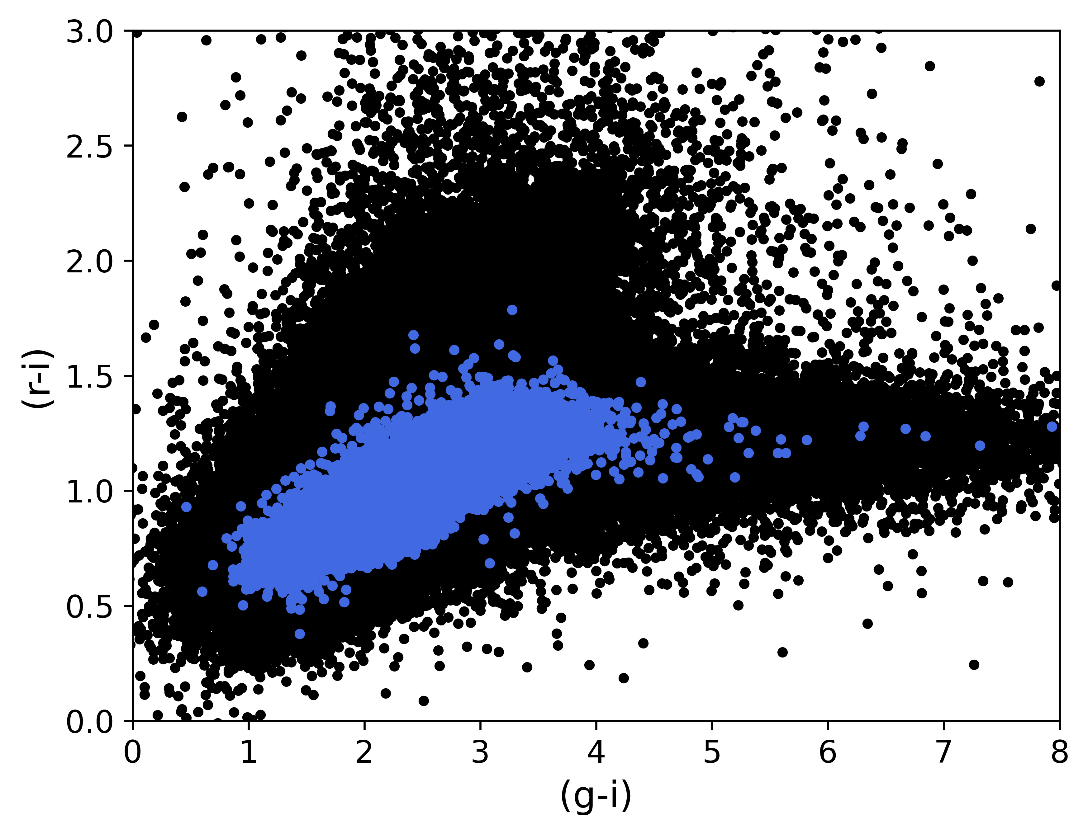
Figure 1: Colours $r-i$ and $g-i$ of the DES galaxies (black) and the matched spec-z sample (blue).

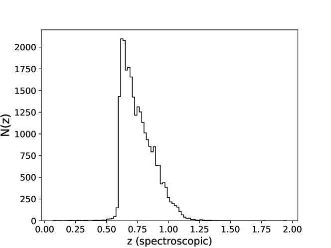
Figure 2: Spec-z sample distribution.

BPZ does not need a training set of spectroscopic redshift, thus the required input information was simply the magnitudes of the galaxies as well as the filters information, we added the DECam filters transmission as a function of wavelength to the BPZ inputs. We chose PDFs with $100$ points and the same redshift range as the chosen for the other algorithms.

We used the same spectroscopic sample described above for DNF/ENF. We also chose 100 points to construct the PDFs. For the specifications with DNF/ENF, we chose 100 neighbours and ensured photometric redshifts remained inside the training redshift range. Because DNF/ENF estimates the redshift according to neighbouring galaxies from the spectroscopic sample, we had to divide the spectroscopic set into $\sim 5000$ training galaxies and the remaining to compute the metrics for these two estimators, otherwise the result would be exactly the spec-z result.

In Table (1), we show the effective redshift $z_{eff}$ defined in [24] and the 68th percentile of the redshift error $\sigma_{z}$, defined as

$$\sigma_{z}=\frac{(z_{p}-z)}{(1+z)}.$$ (2.4)

The comparison was made with the spectroscopic dataset used from training and testing. For ANNz2, we used the set separated to test for the algorithm pipeline. The BPZ bias was calculated with all the available spectroscopic observations. Lastly, for DNF/ENF, we had to run the estimator with the galaxies of the training set, since DNF/ENF does not have a testing step. We separated 80% for training and 20% for testing DNF/ENF, and the 20% was used to compute the bias between redshifts. DNF/ENF’s $\sigma_{z}^{68}$ matches the results obtained by [17] in the incomplete training set case, which means we are providing sufficient spectroscopic reference galaxies.

Data	$z_{eff}$	$\sigma_{z}^{68}$
ANNz2	0.856	${}^{+0.007}_{-0.021}$
BPZ	0.848	${}^{+0.009}_{-0.039}$
ENF	0.854	${}^{+0.018}_{-0.016}$
DNF	0.819	${}^{+0.054}_{-0.016}$

Table 1: Each survey with its effective redshift $z_{eff}$.

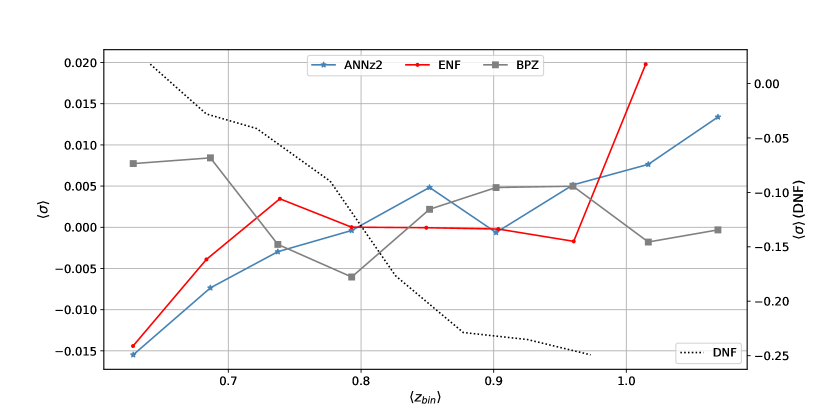
Figure 3: $\sigma_{68}$ of each photo-z estimator. The DNF’s bias is shown in the right y-axis.

3 Bias per redshift bin

A good way to compare these estimates is the quantity $\sigma_{68}$, which is the $68\%$ confidence region of the bias $\sigma$:

$$\sigma=z_{photo}-z_{train}.$$ (3.1)

We plot the bias, Eq. (3.1), per redshift bin in Figure (3), the sample used to compare is the same of the previous plots. The red squares represent the ENF bias per bin, they are larger for $z>0.95$, this is expected once we do not have enough galaxies with these redshift values. The same is true for ANNz2, but the bias is smaller indicating a better performance of this estimator. DNF is the most biased estimator for most bins. Compared to the DES Collaboration results in [15], we agree that in the bins around $z_{p}=0.8$, the bias increases at $z_{p}>1.0$.

In Table (1), we show the effective redshift $z_{eff}$ described by [24], and the 68th percentile of the redshift error $\sigma_{z}$, defined as

$$\sigma_{z}=\frac{(z_{p}-z)}{(1+z)}.$$ (3.2)

The comparison was made with the spectroscopic dataset used from training and testing. For ANNz2, we used the set separated to test for the algorithm pipeline. The BPZ bias was calculated with the available spectroscopic observations. Lastly, for ENF/DNF, we had to run the estimator with the galaxies of the training set, since ENF/DNF does not have a testing step. We separated 80% for training and 20% for testing ENF/DNF, the 20% was used to compute the bias between redshifts.

4 Results

Our results for the four methods are available at the Zenodo repository with DOI: 10.5281/zenodo.14290701. In Figure 4, we show the ANNz2 testing sample compared to the resulting photo-z. The cyan dotted line shows the $\sigma_{99}$ error, the dashed blue line represents the $\sigma_{68}$ error with the expected result. The black and white pixels represent the number of galaxies concentrated with that particular spec-z/photo-z value. The resulting redshift estimation was satisfactory, the sample distribution matches the spectroscopic redshift pattern without much dispersion.

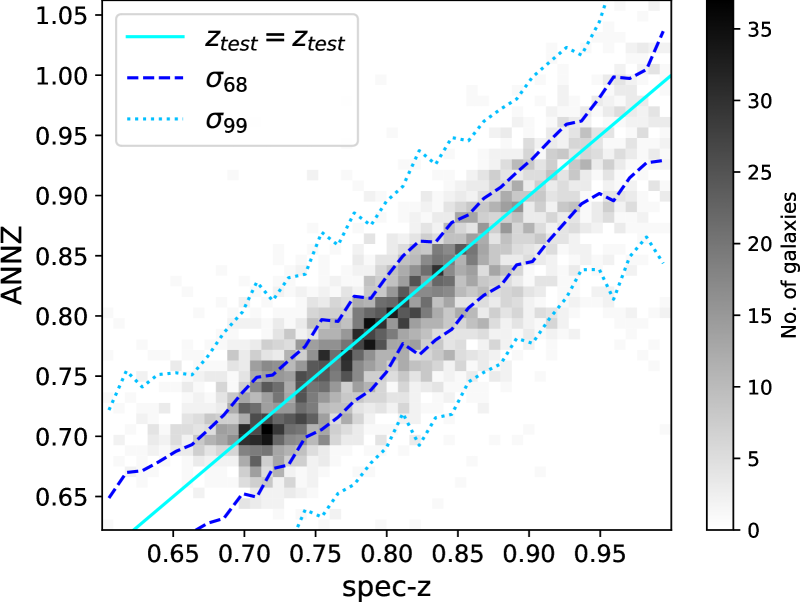
Figure 4: ANNz2 photo-z compared to the spectroscopic training set. The horizontal axis is the spec-z testing sample.

Figure 5 shows the high bias between the BPZ photo-z and the matched samples $spec-z$. Compared to ANNz2, this estimator has a bigger error, indicated by the wider $\sigma_{68}$ region. The results are consistent with the expected redshift, with little dispersion from the $z_{p}=z_{spec}$ line. For redshifts higher than 1.1, $\sigma_{99}$ deviates from a straight line. The stripped pattern is due to the limitation of the estimator of setting a redshift resolution, we chose a resolution of $0.02$. This same pattern can be seen in other studies using BPZ, like in [25].

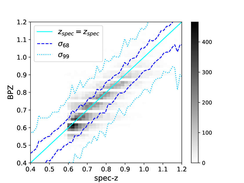
Figure 5: BPZ vs Vipers redshift results.

Paper	Algorithm	$\sigma_{68}$	Sample	Training set size
DES SV [16]	ANNz2 (test 1 cut)	$\sim$0.049	DES SV	7,249
DES SV [16]	BPZ (test 1)	$\sim$0.056	DES SV	-
DES SV [16]	DESDM (test 1)	$\sim$0.055	DES SV	7,249
DES Deep Field [17]	DNF Complete	0.0373	DESY3 Deep Field	26,883
DES Deep Field [17]	DNF Incomplete	0.0500	DESY3 Deep Field	22,651

Table 2: Photo-z estimation using DES objects.

The ENF results are shown in Figure 6. This time the deviation in the errors region happens at $z\sim 0.95$, this indicates that the estimator is not accurate enough for higher redshift values. Finally in Figure 7, DNF seems to overestimate the redshift and has the same issue at higher redshift as ENF. Both algorithms show an asymmetric distribution, the negative $\sigma_{68}$ is closer to the $z_{spec}=z_{p}$ function for the $z<0.9$, these algorithms are overestimating the galaxy’s photo-z. A similar discrepancy appeared in the lower redshift region in [26] for the Sloan Digital Sky Survey photometric catalog.

In table 2, we included results using DES data with different algorithms, from the Scientific Verification and Deep Field. We had to estimate the $\sigma_{68}$ from [17] to the equivalent version of our definition. Our results show lower $\sigma_{68}$ than most cases. The exception is DNF Complete training (all the available filters from DECAM) set from [17]. Compared to [17]’s DNF incomplete case (only $g,r,i,z$ filters like the BAO sample), we found compatible results.

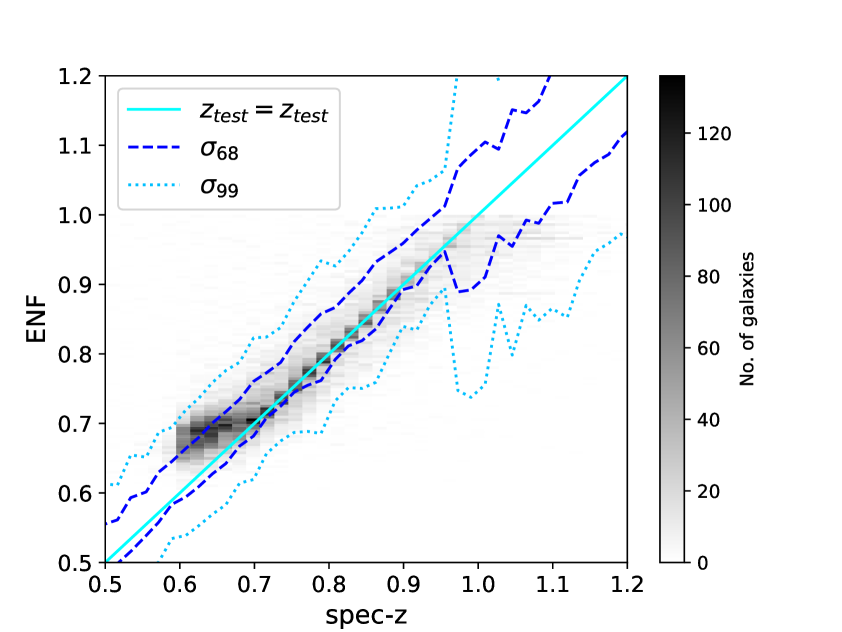
Figure 6: ENF photo-z vs Vipers redshift results.

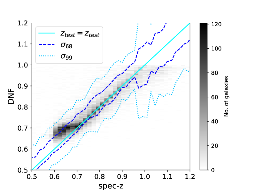
Figure 7: DNF photo-z vs Vipers redshift results.

In order to make sure our spectroscopic sample was enough for DNF, we compare, in Figure 8, our result in the x-axis with the BAO sample by the DES Y3 [19] in the y-axis. They are highly correlated for all the redshift values. The DES Collaboration used $\sim 2.2\times 10^{5}$ spectroscopic matched galaxies in their estimation spectra matched [19]. Despite their superior access to spectroscopic data, our analysis is comparable with $\langle\sigma\rangle=z_{Pz\,\,cats}-z_{DESY3}=-0.003$. Figure 8 shows the 68th percentile for this bias with the same colour scheme used above. The results diverge for $z>0.9$, this means DNF is more sensitive to the training set in this range.

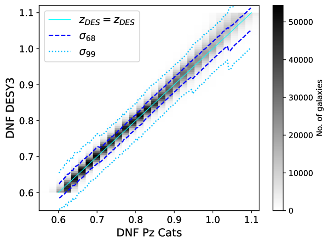
Figure 8: DNF results with our training set and the DESY3 one.

4.1 Consistency tests based on the redshift Probability Distribution Function

Due to the lack of a bigger number of filters, we may find redshift Probability Distribution Functions (PDF) that are not perfect, such as a Dirac delta function. An accurate but not free-of-systematics PDF ideally looks like a Gaussian distribution, and the realistic case results in a survey with nearly Gaussian and multi-modal PDFs.

Photo-z estimator	Method	No. of galaxies	$z_{eff}$	$\sigma_{z}^{68}$
ANNz2	Gaussian PDFs	$2,931,677$	$0.817$	${}^{+0.014}_{-0.031}$
ANNz2	Small peaks	$5,133,775$	$0.799$	${}^{+0.009}_{-0.022}$
ENF	Gaussian PDFs	$299,427$	$0.834$	${}^{+0.040}_{-0.084}$
ENF	Small peaks	$2,256,616$	$0.768$	${}^{+0.046}_{-0.055}$
DNF	Gaussian PDFs	$2,111,461$	0.868	${}^{+0.116}_{-0.121}$
DNF	Small peaks	$2,456,190$	$0.761$	${}^{+0.033}_{-0.142}$
BPZ	Gaussian PDFs	$3,973,671$	$0.812$	${}^{+0.016}_{-0.045}$
BPZ	Small peaks	$5,904,860$	$0.811$	${}^{+0.008}_{-0.042}$

Table 3: All the cuts for each estimator.

Unfortunately, one cannot eliminate all the objects with secondary peaks, but it is possible to exclude the most noisy ones. Here, we computed the number of peaks per PDF and selected galaxies that contain a peak that cannot be larger than 30% of the main peak. Furthermore, we selected PDFs close to a Gaussian distribution. We calculated the statistical moments $\mu_{n}$ using the distributions $PDF(z_{p})$:

$$\mu_{n}=\int\limits_{-\infty}^{\infty}z_{p}^{n}PDF(z_{p})\differential z_{p},$$ (4.1)

where $n$ is the moment ordinal, we use the second moment to classify the distribution. For a Gaussian, the second moment is the sum of the average value squared and the variance ($\mu^{2}+\sigma^{2}$). The mode and the mean are the same in a normal distribution, so we use the $z_{p}$ output of the estimators as $\mu$ and its respective error as $\sigma$. This sample we call Gaussian + "estimator". We shall call Small Peaks the case where the second biggest maximum is not bigger than thirty per cent of the global maximum, this guarantees that the noise is not dominant in the PDF.

The resulting sub-samples are shown in the table 3. BPZ has the biggest number of selected objects. However, because of the Bayesian method, this estimator forces smoother PDFs, but that may not mean it is the best representation of all galaxies, we need to trust that the template available is representative enough of the galaxy’s photometry. ANNz2 shows better precision despite not having a sample as big as BPZ’s. ENF has the worst selection of Gaussian PDFs, with very few galaxies left for a LSS study. Lastly, the worst in precision is DNF but with sufficient galaxies for cosmological analysis. The Small Peaks results are more populated, this time ANNz2 has better precision and more objects than the other algorithms. Choosing the least noisy PDFs may be an advantage to LSS studies for being less selective because the decrease in the number of objects is lower.

From eq. (3.1) 68th percentile, we plot the distribution of $\sigma_{z}$ for all the estimators and sample cuts. In Figure 9, we show the distribution of $\sigma_{z}$ for all the samples described here. The black line represents the whole survey, the blue one represents the samples only with Gaussian PDFs, and the grey area includes multi-modal PDFs but not too noisy.

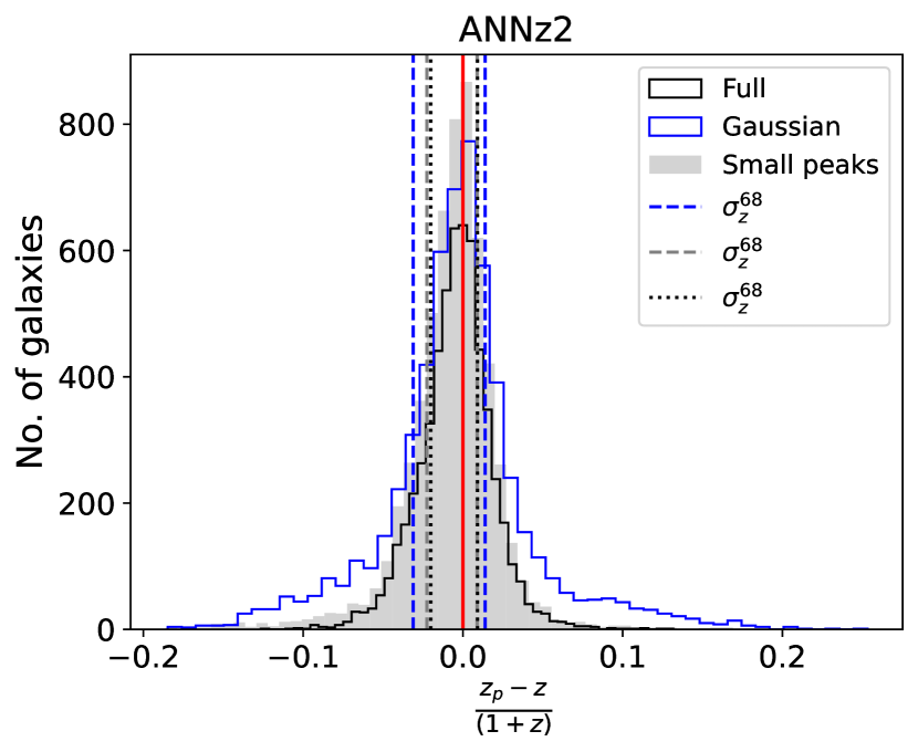
(a) ANNZ $\sigma_{z}$

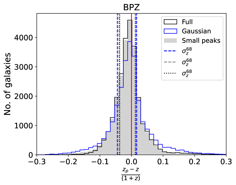
(b) BPZ $\sigma_{z}$

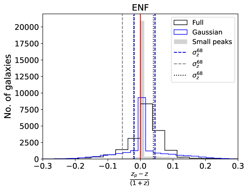
(c) ENF $\sigma_{z}$

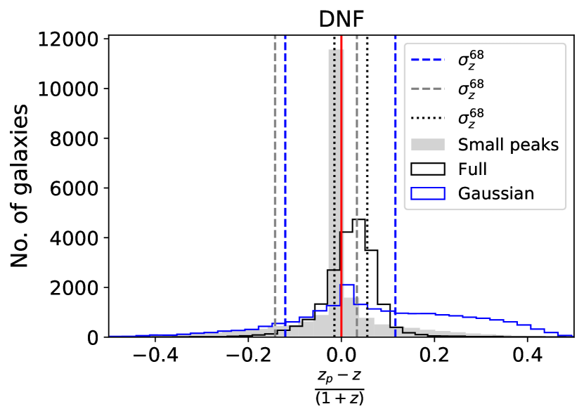
(d) DNF $\sigma_{z}$

Figure 9: Comparison of $\sigma_{z}$ values from different models.

The first panel has the ANNz2 normalised bias, Figure 9(a), the vertical lines respecting the distribution colours. The expected normalised bias is a Gaussian distribution with mean zero, the three cases show the centres close to zero, but the distributions are not perfectly Gaussian, and the $\pm\sigma_{68}$ are not symmetric. The least accurate sample is the blue (Gaussian) one, the main reason is the loss of statistics. In Figure 9(b), BPZ’s three distributions are very similar and not Gaussian. ENF and DNF (Figure 9(c),9(d)) have the worst normalised bias distribution and biggest $\pm\sigma_{68}$.

4.2 Precision with respect to the redshift

Complementary to the results above, we show $\sigma_{68}$ w.r.t. the spectroscopic redshift of the matched galaxies used for testing (all galaxies for BPZ). The result is shown in Figure 10. BPZ in figure 10(a) looses precision when $z>1.0$, for ENF/DNF(figs. 10(c),10(d)) this happens at $z>0.9$. The only photo-z estimator to show consistent and precise results is ANNz2.

(a) BPZ

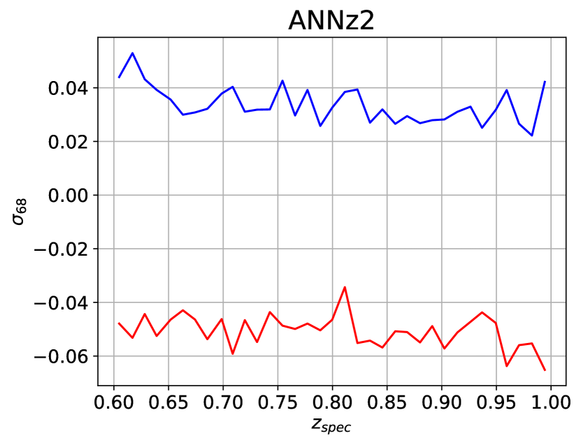
(b) ANNz2

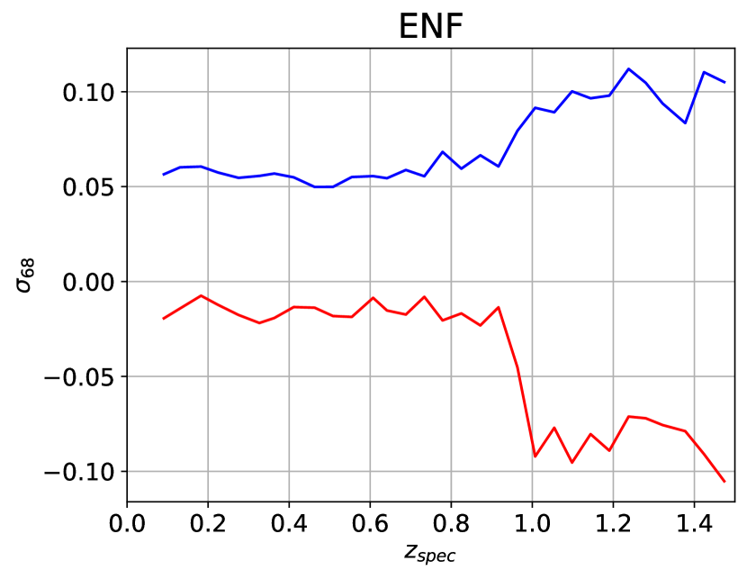
(c) ENF

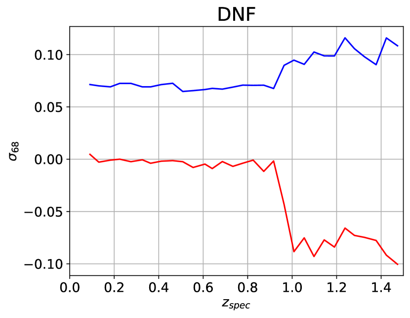
(d) DNF

Figure 10: $\sigma^{68}$ for each $z_{spec}$ bin. Blue: positive error. Red: negative error.

This is consistent with Figures 4, 5, 6, and 7. The asymmetry of overestimation by ENF/DNF and underestimation by BPZ, while ANNz2 is nearly uniform for all redshift values.

We know there are certain galaxies that are not well estimated giving catastrophic redshift. Here, we choose $\sigma_{z}>\sigma_{99}$ as a catastrophic result. In table 4 we compare the numbers of galaxies with catastrophic results, ANNz2 has the best performance compared to the other estimators. Then, we compared the PDF performance in the catastrophic results, BPZ distribution modes $z_{mode}$ match exactly the photo-z result, but the other algorithms show discrepancy, with ANNz2 as with the worst result.

Estimator	# of galaxies with $\sigma_{z}>\sigma_{99}$	# of galaxies with $|z_{mode}-z_{phot}|>0.1$
ANNz2	146	81
BPZ	1,283	0
ENF	1,179	38
DNF	1,084	27

Table 4: Catastrophic results for each algorithm.

We compared the relative frequency of galaxies classified with Gaussian PDFs from the testing sample for each algorithm. In Figure 11, we show the number of Gaussians ($N_{Gauss}$) up to $|\sigma_{z}|$ compared to the number of galaxies in the test sample up to $|\sigma_{z}|$. BPZ has nearly 70% Gaussian PDFs with bias bigger than 0.075 and ANNz2 has nearly 60%. ENF reaches a maximum of 25% of Gaussian PDFs for very small bias, after $|\sigma_{z}|>0.025$, the frequency saturates and only 15% of the PDFs are nearly Gaussian. The opposite happens to DNF, it is an improvement compared to ENF, but saturation is below 25%. This result shows an important situation that may occur, even though the PDFs are smooth, there are catastrophic redshift results.

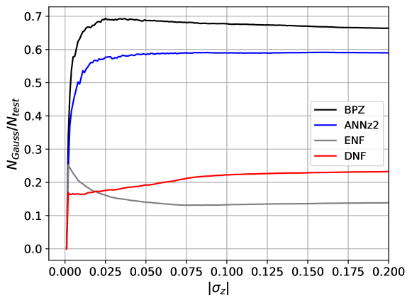
Figure 11: Relative frequency of Gaussian distributions compared to the total number of testing samples w.r.t. the absolute bias ($\sigma_{z}$) for each estimator.

4.3 Filters with respect to the bias

Another important aspect is how $\sigma_{68}$ behaves for each filter. We chose to analyse the behaviour for magnitudes greater than 20. First, we compare the bias normalized by $\sigma_{68}$ in Figure 12. The first panel shows the distribution for the filter $g$, because DNF has the larger error, the distribution (in red) is narrower than the other estimators. ANNz2 and BPZ are centred at zero. DNF and ENF are centred at positive bias. The same pattern is seen in the second top panel for the filter $r$. The filters $i$ and $z$ show a different pattern, ANNz2 is still centred at zero, while BPZ is centred at negative bias and DNF at positive bias. ENF’s filter $i$ is less positive than the other filters. Finally for filter $z$, in the last panel, the only difference from the previous one is BPZ’s distribution which is now more negative.

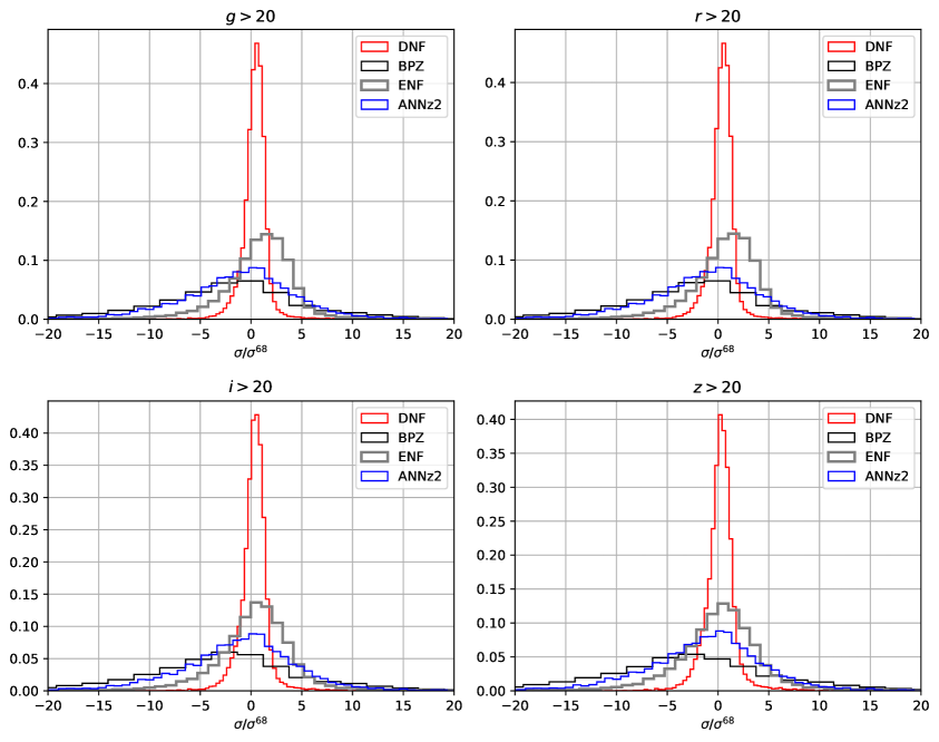
Figure 12: Bias distribution for each filter. Red: DNF, black: BPZ, gray: ENF and blue: ANNz2.

Therefore, the best estimator is ANNz2, its error is consistent for all redshifts. The other estimators are less precise for higher redshift. For LSS analysis this is problematic, the ideal scenario should include a wider range of redshifts.

4.4 Colour cut

In the previous test, we based our $\sigma_{68}$ analysis w.r.t. the colour coverage of our spectroscopic sample, in Figure 1. For each estimator, we cut the redshifts restriction to the colours $1<g-i<4$ and $0.5<r-i<1.4$. Then, we selected the redshifts whose $\sigma_{68}$ is smaller than $10\%$ of the photo-z value. In table 5, there are the $z_{eff}$ considering the colour cut and it is clear that they are compatible with the entire sample photo-z estimation. lastly, the number of objects reduces significantly to DNF, so depending on the use of the catalog, one must understand that an accurate representation of the filters by the training sample may reduce statistics.

Estimator	$z_{eff}$	number of galaxies
ANNz2	0.86	7,031,738
BPZ	0.84	7,012,076
ENF	0.82	6,304,106
DNF	0.84	4,727,115

Table 5: Result after the colour cut.

We checked the bias distribution normalized by $\sigma_{68}$ in terms of the faintest part of each filter. This is shown in Figure 12, the only algorithm that is symmetric over the bias is ANNz2, BPZ underestimates the faint galaxies, while DNF and ENF overestimate them.

5 Summary

This study explored the properties of four different photo-z estimators: ANNz2, BPZ, ENF, DNF with the same spectroscopic sample to train and/or test their precision.

We selected 25,760 galaxies from four different spectroscopic surveys and cross-matched them with the DES Y3 BAO sample. These galaxies served to understand the redshift bias $\sigma$ and its 68th percentile $\sigma_{68}$ and are representative in terms of magnitude. We found that within a range of $0.79<z_{p}<0.85$ there is the lowest $\sigma$ for all the estimators we analysed. DNF has the biggest absolute value of the bias, while ENF, ANNz2 and BPZ lose precision for a redshift range below 0.7 and higher than 0.9.

Computing the statistical metrics of the redshfit errors we found that the smallest bias belong to BPZ and the worst bias belongs to DNF. The least biased bin is $z_{p}\sim 0.8$ for all estimators, while the most biased bins are below 0.7 and above 0.9.

We also investigated the $\sigma_{68}$ metric, a robust metric to estimate the error of the algorithms. ANNz2 and BPZ showed consistent $\sigma_{68}$ for all bins, while ENF and DNF have an asymmetric error distribution, with lower negative error values than the positive ones and a considerable error increase for redshift higher than 0.9. As a consistent test, we compared with the DES Collaboration, because our and their results diverge slightly for higher redshift, we conclude that this algorithm is sensitive to the training set available especially in the high redshift end.

The other test we conducted involved selecting the best galaxies according to their redshift PDFs. The resulting sub-samples gave BPZ with the biggest number of selected objects. However, because of the Bayesian method, this estimator forces smoother PDFs. ANNz2 shows better precision despite not having a sample as big as BPZ’s. ENF has the worst selection of Gaussian PDFs, with very few galaxies left for an LSS study. Lastly, worst in precision lies DNF but with sufficient galaxies for cosmological analysis. For the Small Peaks sub-sample, ANNz2 performed better than the other algorithms. Due to the highly selective criteria, the Gaussian sub-sample is not ideal for studies that need significant statistics, this will be demonstrated in a following study using Pz Cats.

In case one wants to pick the best galaxies by removing the bins with the worst bias, they will find that ANNz2 is the most robust algorithm for all criteria. DNF and ENF have a significant shift from zero. We also showed that even though the PDFs are smooth, there are catastrophic redshift results.

Lastly, we analysed how the bias behaves with faint galaxies. The result confirmed the other analysis, where ANNz2 is consistent for all redshifts, while the other estimators overestimate or underestimate the photo-zs. In the end, of the four algorithms ANNz2 was successful in most of the metrics discussed with less catastrophic results. In the next study, we will show whether this success influences cosmological results.

References

- [1] S. Arnouts, S. Cristiani, L. Moscardini, S. Matarrese, F. Lucchin, A. Fontana et al., Measuring and modelling the redshift evolution of clustering: the hubble deep field north, Monthly Notices of the Royal Astronomical Society 310 (1999) 540.
- [2] L. Guzzo, M. Scodeggio, B. Garilli, B. Granett, A. Fritz, U. Abbas et al., The vimos public extragalactic redshift survey (vipers)-an unprecedented view of galaxies and large-scale structure at 0.5< z< 1.2, Astronomy & Astrophysics 566 (2014) A108.
- [3] N. Benitez, Bayesian photometric redshift estimation, The Astrophysical Journal 536 (2000) 571.
- [4] R. Feldmann, C.M. Carollo, C. Porciani, S. Lilly, P. Capak, Y. Taniguchi et al., The zurich extragalactic bayesian redshift analyzer and its first application: Cosmos, Monthly Notices of the Royal Astronomical Society 372 (2006) 565.
- [5] G.B. Brammer, P.G. van Dokkum and P. Coppi, Eazy: a fast, public photometric redshift code, The Astrophysical Journal 686 (2008) 1503.
- [6] M. Carrasco Kind and R.J. Brunner, Tpz: photometric redshift pdfs and ancillary information by using prediction trees and random forests, Monthly Notices of the Royal Astronomical Society 432 (2013) 1483 [https://academic.oup.com/mnras/article-pdf/432/2/1483/18463634/stt574.pdf].
- [7] I. Sadeh, F.B. Abdalla and O. Lahav, Annz2: photometric redshift and probability distribution function estimation using machine learning, Publications of the Astronomical Society of the Pacific 128 (2016) 104502.
- [8] I.A. Almosallam, M.J. Jarvis and S.J. Roberts, Gpz: non-stationary sparse gaussian processes for heteroscedastic uncertainty estimation in photometric redshifts, Monthly Notices of the Royal Astronomical Society 462 (2016) 726.
- [9] J. De Vicente, E. Sánchez and I. Sevilla-Noarbe, Dnf–galaxy photometric redshift by directional neighbourhood fitting, Monthly Notices of the Royal Astronomical Society 459 (2016) 3078.
- [10] N. Padmanabhan, T. Budavári, D.J. Schlegel, T. Bridges, J. Brinkmann, R. Cannon et al., Calibrating photometric redshifts of luminous red galaxies, Monthly Notices of the Royal Astronomical Society 359 (2005) 237.
- [11] H. Hoshino, A. Leauthaud, C. Lackner, C. Hikage, E. Rozo, E. Rykoff et al., Luminous red galaxies in clusters: central occupation, spatial distributions and miscentring, Monthly Notices of the Royal Astronomical Society 452 (2015) 998.
- [12] D.J. Eisenstein, J. Annis, J.E. Gunn, A.S. Szalay, A.J. Connolly, R. Nichol et al., Spectroscopic target selection for the sloan digital sky survey: The luminous red galaxy sample, The Astronomical Journal 122 (2001) 2267.
- [13] R. McMahon, The vista hemisphere survey (vhs) science goals and status, Science from the Next Generation Imaging and Spectroscopic Surveys 37 (2012) .
- [14] M. Banerji, S. Jouvel, H. Lin, R. McMahon, O. Lahav, F. Castander et al., Combining dark energy survey science verification data with near-infrared data from the eso vista hemisphere survey, Monthly Notices of the Royal Astronomical Society 446 (2015) 2523.
- [15] I. Sevilla-Noarbe, K. Bechtol, M.C. Kind, A.C. Rosell, M. Becker, A. Drlica-Wagner et al., Dark energy survey year 3 results: Photometric data set for cosmology, The Astrophysical Journal Supplement Series 254 (2021) 24.
- [16] C. Sánchez Alonso, M. Carrasco Kind, H. Lin, M. Serra Ricart, F.B. Abdalla, A. Amara et al., Photometric redshift analysis in the dark energy survey science verification data, Monthly notices of the Royal Astronomical Society. Oxford. Vol. 445, no. 2 (Dec. 2014), p. 1482-1506 (2014) .
- [17] L.T. San Cipriano, J. De Vicente, I. Sevilla-Noarbe, W. Hartley, J. Myles, A. Amon et al., Dark energy survey deep field photometric redshift performance and training incompleteness assessment, Astronomy & Astrophysics 686 (2024) A38.
- [18] A.A. Collister and O. Lahav, Annz: estimating photometric redshifts using artificial neural networks, Publications of the Astronomical Society of the Pacific 116 (2004) 345.
- [19] T. Abbott, M. Aguena, S. Allam, A. Amon, F. Andrade-Oliveira, J. Asorey et al., Dark energy survey year 3 results: A 2.7% measurement of baryon acoustic oscillation distance scale at redshift 0.835, Physical Review D 105 (2022) 043512.
- [20] M. Scodeggio, L. Guzzo, B. Garilli, B. Granett, M. Bolzonella, S. De La Torre et al., The vimos public extragalactic redshift survey (vipers)-full spectroscopic data and auxiliary information release (pdr-2), Astronomy & Astrophysics 609 (2018) A84.
- [21] J.A. Newman, M.C. Cooper, M. Davis, S. Faber, A.L. Coil, P. Guhathakurta et al., The deep2 galaxy redshift survey: Design, observations, data reduction, and redshifts, The Astrophysical Journal Supplement Series 208 (2013) 5.
- [22] O. Le Fèvre, G. Vettolani, B. Garilli, L. Tresse, D. Bottini, V. Le Brun et al., The vimos vlt deep survey-first epoch vvds-deep survey: 11 564 spectra with 17.5 i 24, and the redshift distribution over 0 z 5, Astronomy & Astrophysics 439 (2005) 845.
- [23] Y. Wang, G.-B. Zhao, C. Zhao, O.H. Philcox, S. Alam, A. Tamone et al., The clustering of the sdss-iv extended baryon oscillation spectroscopic survey dr16 luminous red galaxy and emission-line galaxy samples: cosmic distance and structure growth measurements using multiple tracers in configuration space, Monthly Notices of the Royal Astronomical Society 498 (2020) 3470.
- [24] A.J. Ross, N. Banik, S. Avila, W.J. Percival, S. Dodelson, J. Garcia-Bellido et al., Optimized clustering estimators for bao measurements accounting for significant redshift uncertainty, Monthly Notices of the Royal Astronomical Society 472 (2017) 4456.
- [25] V. Margoniner and D. Wittman, Photometric redshifts and signal-to-noise ratios, The Astrophysical Journal 679 (2008) 31.
- [26] R.R.R. Reis, M. Soares-Santos, J. Annis, S. Dodelson, J. Hao, D. Johnston et al., The sloan digital sky survey co-add: A galaxy photometric redshift catalog, The Astrophysical Journal 747 (2012) 59.