Explainable Time Series Prediction of
Tyre Energy in Formula One Race Strategy

Abstract.

Formula One (F1) race strategy takes place in a high-pressure and fast-paced environment where split-second decisions can drastically affect race results. Two of the core decisions of race strategy are when to make pit stops (i.e. replace the cars’ tyres) and which tyre compounds (hard, medium or soft, in normal conditions) to select. The optimal pit stop decisions can be determined by estimating the tyre degradation of these compounds, which in turn can be computed from the energy applied to each tyre, i.e. the tyre energy. In this work, we trained deep learning models, using the Mercedes-AMG PETRONAS F1 team’s historic race data consisting of telemetry, to forecast tyre energies during races. Additionally, we fitted XGBoost, a decision tree-based machine learning algorithm, to the same dataset and compared the results, with both giving impressive performance. Furthermore, we incorporated two different explainable AI methods, namely feature importance and counterfactual explanations, to gain insights into the reasoning behind the forecasts. Our contributions thus result in an explainable, automated method which could assist F1 teams in optimising their race strategy.

1. Introduction

Formula One (F1) is a popular sport all over the globe, with some Grand Prix races exceeding 100 million TV viewers. The significant prize pools mean that competing teams will go to great lengths to maximise the performance of their cars. Because of this, analysing historical race data is essential for teams as they provide useful insights into how various factors affect the car performance. One of the most important factors is the tyre degradation, i.e. how different tyre compounds wear and degrade over time, which lowers the grip they provide and thus the car’s speed. This means teams must optimise their strategies in their selection of which tyre compounds to use and when to pitstop, i.e. leave the race to change tyres. A major contributor to the rate of tyre degradation is the fluctuating energy applied to each tyre, i.e. the tyre energy. This energy represents the sliding power, which is calculated using a physics-based model, comprising variables such as the forces on the tyre and the slip velocity. AI models have not as of yet, as far as we are aware, been used in F1 to forecast tyre degradation. The industry standard for predicting this phenomenon is using simple linear models, which are clearly trustworthy but are often manually calculated and thus time-consuming, and do not take covariate data into account.

Meanwhile, sophisticated time series prediction models such as Long Short-Term Memory (LSTM) (Hochreiter and Schmidhuber, 1997) and Transformers (Vaswani et al., 2017) have been shown to accurately predict future unseen data when given historical multivariate data. It is therefore feasible that such a model could map car telemetry data such as speed and steering wheel angle into an estimation of the tyre energies at any given time. However, time series prediction models lack the ability to explain their forecasts to users. Given the high-risk nature of F1, race strategists would be highly unlikely to trust such an unaccountable model, since it is ultimately the strategist who would need to justify any decisions taken based on this information. However, explainable AI (XAI) techniques have been shown to provide explanations of forecasts from time-series models (see (Rojat et al., 2021) for a recent survey), thus fostering trust from users towards the models.

In this work, we trained and optimised four different deep learning models, consisting of three different Recurrent Neural Network (RNN) models and a state-of-the-art Transformer-based model, to forecast tyre energies for an arbitrary race, given a set of covariate data, e.g. brake, throttle and steering wheel angle from the car’s telemetry. In addition, we incorporated two baselines: linear regression and XGBoost, a gradient-boosted decision tree ensemble algorithm (Chen and Guestrin, 2016). Furthermore, we tested alternative deployments of these prediction models such as single-track specialists and regression-based models to determine the optimal model for real-world use. Finally, we integrated two XAI algorithms, TIME (Sood and Craven, 2022) and CausalImpact (Brodersen et al., 2015), to provide insights into the predictions of our deep learning models. While XGBoost was the most accurate at forecasting our test set, we find the results of our deep learning models to be promising. Furthermore, the integrated XAI methods offer rational and encouraging explanations for the predictions. Our work makes steps towards the real-world use of AI models in F1 for processing live data and predicting tyre energies during a race.

2. Related Work

Time series prediction (also referred to as time series forecasting) concerns training a model to predict the future values of targets based on their previously observed values and/or that of covariates. These covariates are external variables that can be used as inputs to help improve the accuracy of predictions.

Various deep learning architectures have been integrated into time series forecasting. RNNs have been the basis of many forecasting models, such as DeepAR by Salinas et al. (Salinas et al., 2017). The LSTM architecture (Hochreiter and Schmidhuber, 1997), a specialised form of RNN, has shown great potential in applying time series forecasting in fields such as macroeconomics (Kamolthip, 2021) and iron-making (Schockaert et al., 2020). Transformers (Vaswani et al., 2017), which were designed to handle sequence-to-sequence tasks, also see effective use in forecasting time series. PatchTST by Nie et al. (Nie et al., 2023), a Transformer-based model, was the first to be trained on “patched” time series, where the input series is divided into equal-sized patches, inspiring other models such as TSMixer (Ekambaram et al., 2023), a lightweight model composed entirely of multi-layer perception modules. Meanwhile, the Temporal Fusion Transformer (TFT) by Lim et al. (Lim et al., 2019) pushed the state-of-the-art in terms of both accuracy and innovation, consisting of an interpretability module, allowing insights such as feature importance to be analysed. Despite this, studies have shown that Transformer-based models may not be as effective at time series forecasting as previously thought, with simple baselines outperforming the state-of-the-art on benchmark datasets (Zeng et al., 2023).

With regards to applications of time series models in the world of motorsport, Schleinitz et al. (von Schleinitz et al., 2021) combined a variational autoencoder (Kingma and Welling, 2014), an anomaly detector and LSTM predictors to propose the variational autoencoder based selective prediction (VASP) framework. VASP was evaluated in the tasks of anomaly detection and robust time series prediction using data from motorsport race series. The framework outperformed the other approaches for this task and coped well even when anomalies were present. However, VASP, unlike our approach, was not deployed for time series prediction of tyre energy in F1.

Our work is not the first to apply machine learning models to predict variables concerning tyres. Zhang et al. (Zhang et al., 2020) developed and trained a neural network to predict the tyre abrasion status in real-time. The tyre wear was predicted based on accelerometer and strain gauge data. All test data was predicted within $\pm 0.5$mm, with 80% of test cases within $\pm 0.2$mm. Meanwhile, Kim et al. (Kim et al., 2023) developed a 1D Convolutional Neural Network (CNN) that predicts tyre wear using various vehicle and tyre sensing information. Results showed that using more input data resulted in better performance overall, with the best models having a prediction error of 0.21mm, although models which only relied on wheel translation and rotation speed were still promising when accounting for sensing cost.

Accurate predictions alone may not warrant the use of such models in high-risk industries, as the models’ lack of interpretability requires users to blindly trust their predictions, which would mean that risks are taken without justification. XAI methods aim to help users understand how AI models compute outputs in an accessible manner (Bhatt et al., 2020). The best XAI methods should be (among other features) interpretable and trustworthy (Rojat et al., 2021), features which would undoubtedly be desirable in this application.

Feature importance is one of the most popular explanation types for tabular data, assigning an importance value to each feature reflecting how significant the feature was when computing the prediction (Bodria et al., 2023). Temporal Importance Model Explanation (TIME) by Sood et al. (Sood and Craven, 2022) is an XAI method based on feature importance that calculates the importance of each input feature for the model at each time step. This is achieved via repeatedly perturbing the input tensor fed to the model and analysing the differences in results, enabling the user to know when and to what degree certain variables contribute to the model’s output.

Counterfactual explanations assess how a model was dependent on external factors when making a particular prediction, focusing on the differences to obtain the opposite prediction (Bodria et al., 2023). CausalImpact by Brodersen et al. (Brodersen et al., 2015) is a method based on counterfactual explanations which infers the impact of an “intervention” (an event that significantly affects future target values) on time series data, achieved by modelling the counterfactual scenario where the intervention did not occur and comparing the difference.

In this paper, we will experiment with both TIME and CausalImpact. To the best of our knowledge, there are no approaches in the literature which apply time series prediction or explainable AI to F1 applications, as we do in this paper.

3. Time Series Forecasting of Tyre Energy

In this section we detail our study, namely: the dataset used (§3.1); the track state encodings (§3.2); how the data was partitioned (§3.3); our problem formulation (§3.4); and the deployed forecasting models and XAI methods (§3.5).

3.1. Time Series Data

We were provided with both serialised and tabular raw data by the Mercedes-AMG PETRONAS F1 Team, taken from real-time sources such as the car telemetry and GPS. After processing, aligning and merging the raw data, we produced a tabular time series of 0.1s resolution for each race and both drivers from the team, covering the 2020 to 2023 seasons. Some events were excluded as will be discussed in §3.3. Each time series contained the following covariates:

• Time into race (float);

• Car speed and its uncertainty (float);

• Lap number (int);

• Distance around track and distance uncertainty (float);

• Steering wheel angle (float);

• Under/oversteer coefficient (float);

• Lift and coast (boolean) and its distance (float);

• Gear (int);

• Brake (percentage from 0-100);

• Throttle (percentage from 0-100);

• Engine speed (float);

• Fuel load (float);

• Track temperature (float);

• Pit stop status (boolean);

• DRS enabled (boolean) and Pod disabled (boolean);

• Track state (categorical, see §3.2).

The target variables were the energies applied to each of the four tyres. Time was measured from the race start (time = 0) until the end of the raw data sources (roughly five seconds after the car crosses the finish line). In addition to the above covariates, the car’s latitude and longitude were stored for visualising model performance around the track, but were not an input to the model.

3.2. Track State Encodings

The track state is a categorical covariate, representing the current race conditions. In F1, green-flag signifies standard conditions, yellow-flag prohibits cars from overtaking due to a minor incident, and red-flag conveys a race suspension, where cars must drive carefully to the pit lane. Safety cars and virtual safety cars deploy in response to track incidents, enforcing cars to adhere to strict speed limits. Thus, the track state significantly influences other covariates, such as car speed, and so four distinct encoding methods were evaluated:

• exclude the track state from the input data entirely;

• one-hot encoding the state;

• encode the state in order based on expected car speed;

• filter the training set to include only time steps where the track state is green-flag, then exclude the track state column.

Early tests gave no outright best method, so all approaches were included in hyperparameter optimisation experiments.

3.3. Dataset Partitioning

Since there are a wide variety of tracks in F1, fixed training, validation and test sets were decided on with the following properties:

• The training, validation and test sets consisted of 20, 6 and 7 events respectively, ranging from the 2020 to 2023 seasons.

• Each event had 2 races, one for each Mercedes driver, with the end of one race being immediately followed by the start of the next race.

• The datasets contained a mixture of faster open tracks and slower street circuits, to explore the models’ adaptability to various environments.

• The validation and test sets contained both seen and unseen tracks. A seen (unseen) track was one the models had (had not, respectively) been trained on from another season.

Races that took place under wet conditions, were suspended, or lacked necessary data were excluded from the datasets.

3.4. Problem Formulation

For each time step of the test set, the time series forecasting model received the previous 100 time steps of input data and needed to forecast the immediate next value for the energies of each tyre (giving four targets in total). Contrary to standard forecasting tasks, the input data contained only covariate values; no past ground truth values for tyre energies were supplied to the model. The model’s objective was to minimise the root mean squared error (RMSE) of the complete test set for the tyre energies.

3.5. Forecasting Models and XAI Methods

The following deep learning models were developed using the PyTorch library for time series forecasting: RNN (Rumelhart et al., 1986), LSTM (Hochreiter and Schmidhuber, 1997) and Gated Recurrent Unit (GRU) (Cho et al., 2014). In addition, the TFT (Lim et al., 2019) was adapted for this task using the PyTorch Forecasting library. Linear regression and XGBoost (Chen and Guestrin, 2016), both statistical approaches, were integrated as baselines.

To provide insight into the models’ predictions, we incorporated both TIME (Sood and Craven, 2022), a temporal Feature Importance algorithm, and CausalImpact (Brodersen et al., 2015), a statistical Counterfactual Explanation method.

4. Evaluation and Discussion

In this section, we evaluate and discuss the results of the time series forecasting models (§4.1) and the incorporated XAI algorithms (§4.2). Our experiments were conducted on a Linux cluster with AMD EPYC 7742 CPU, 1TB RAM, and RTX 6000 GPU.

4.1. Time Series Forecasting

We first performed hyperparameter tuning on the training set to optimise our deep learning models, utilising state-of-the-art algorithms provided by Ray Tune and Optuna (Akiba et al., 2019). The track state encodings were included in the search space for each model, with the exception of the green-flag only encoding, as this would be used as a comparison on the complete test set. The optimal configurations from these experiments are detailed in Table 1.

Table 1. Optimal Configurations from Hyperparameter Search Experiments

Hyperparameter	RNN	LSTM	GRU	TFT
Track State Encoding	One-Hot	Exclude	One-Hot	One-Hot
Gradient Clip Norm	0.721	0.375	0.124	0.811
Hidden Size	256	512	256	32
Learning Rate	0.073	0.002	1e-4	4e-5
Number of Layers	8	8	4	8
Optimiser	SGD	Ranger	AdamW	Adam
Bi-directional	NO	YES	NO	-
Dropout	-	-	-	0.150
# Attention Heads	-	-	-	8

The results for the test set are presented in Table 2. HS Best represents the track state encoding featured in the best configuration from hyperparameter search experiments (from Table 1), while Green-flag represents an identical model with a green-flag encoded dataset. Values in italics highlight the lowest RMSE of the two track state encodings for each model, with the lowest overall highlighted in bold.

Table 2. Baseline and Fine-tuned Deep Learning Model RMSEs on Test Set

Model	Linear	XGBoost	RNN	LSTM	GRU	TFT
HS Best	7.893	4.841	5.926	5.896	5.517	5.693
Green-flag	7.916	4.785	5.697	5.730	5.558	5.305

From the results, one can observe that all neural models vastly outperformed the linear regression baseline, with the TFT producing the most accurate forecasts of the deep learning models. XGBoost outperformed all trained deep learning models by a considerable margin. However, classifying XGBoost as a baseline for this task may be somewhat unfair as it had to fit to the complete training set and thus required far more RAM (of up to 1024 GB) than any of our deep learning models (at most 256 GB).

Regardless, XGBoost’s performance was very promising, as shown in Figure 1, which also displays the TFT’s forecasts over the same race and lap for comparison. XGBoost captures the trends of the lap far more closely than the TFT. Figure 2 further demonstrates this on an unseen street circuit, showcasing XGBoost’s adaptability to new (types of) tracks.

Figures 3 and 4 demonstrate the performance of XGBoost and TFT over the Abu Dhabi Grand Prix, a seen open track, and the Miami Grand Prix, an unseen street circuit, respectively. These plots highlight the symmetric mean absolute percentage error (SMAPE), a proportional error metric ranging from 0 to 100, allowing us to determine the strongest and weakest sections of the tracks. XGBoost has far fewer sections of the Abu Dhabi track with high SMAPE compared to the TFT, although the difference between the two is less significant for the Miami track. Most weak sections are either during, or shortly preceding or following a corner, which is reasonable as tyre energies change rapidly during these moments.

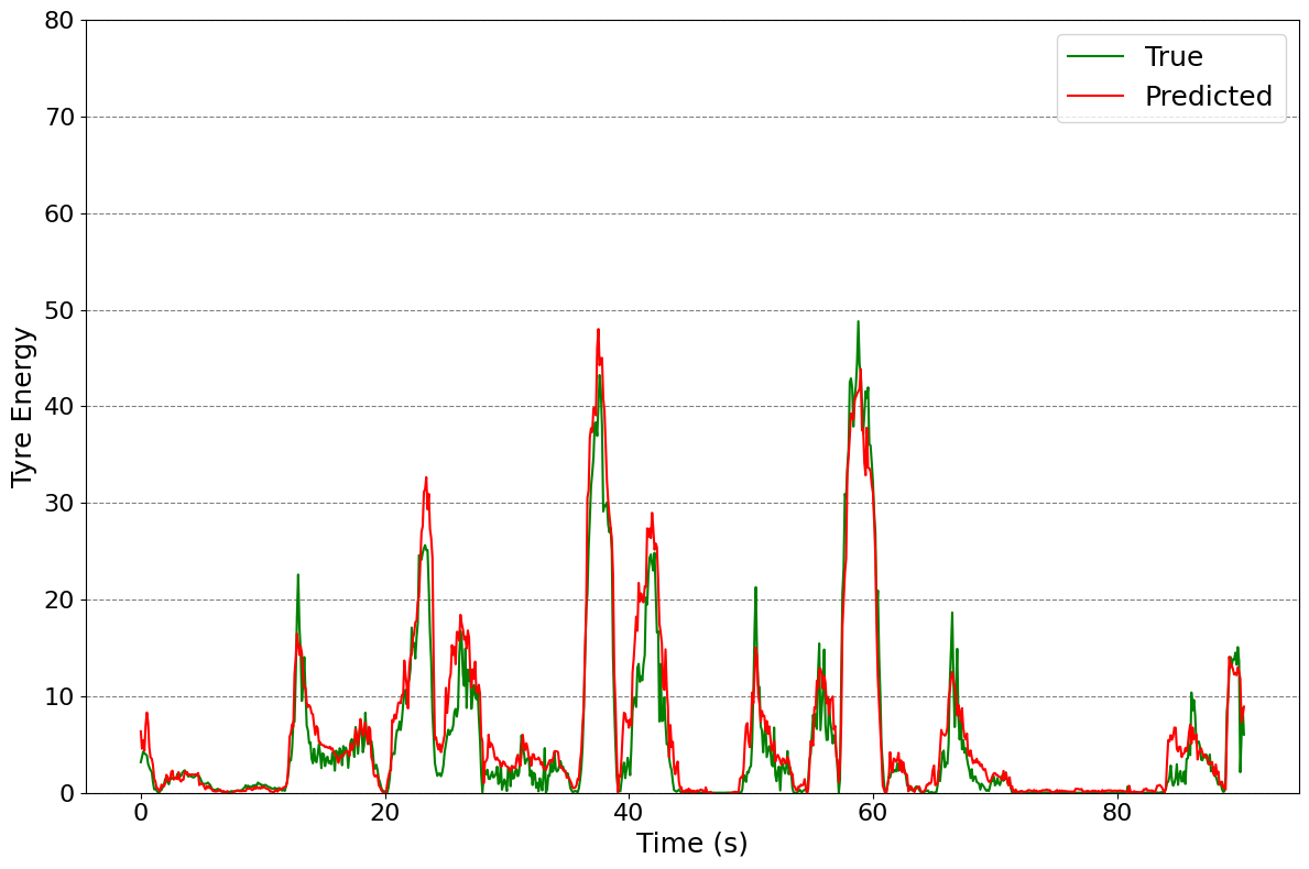
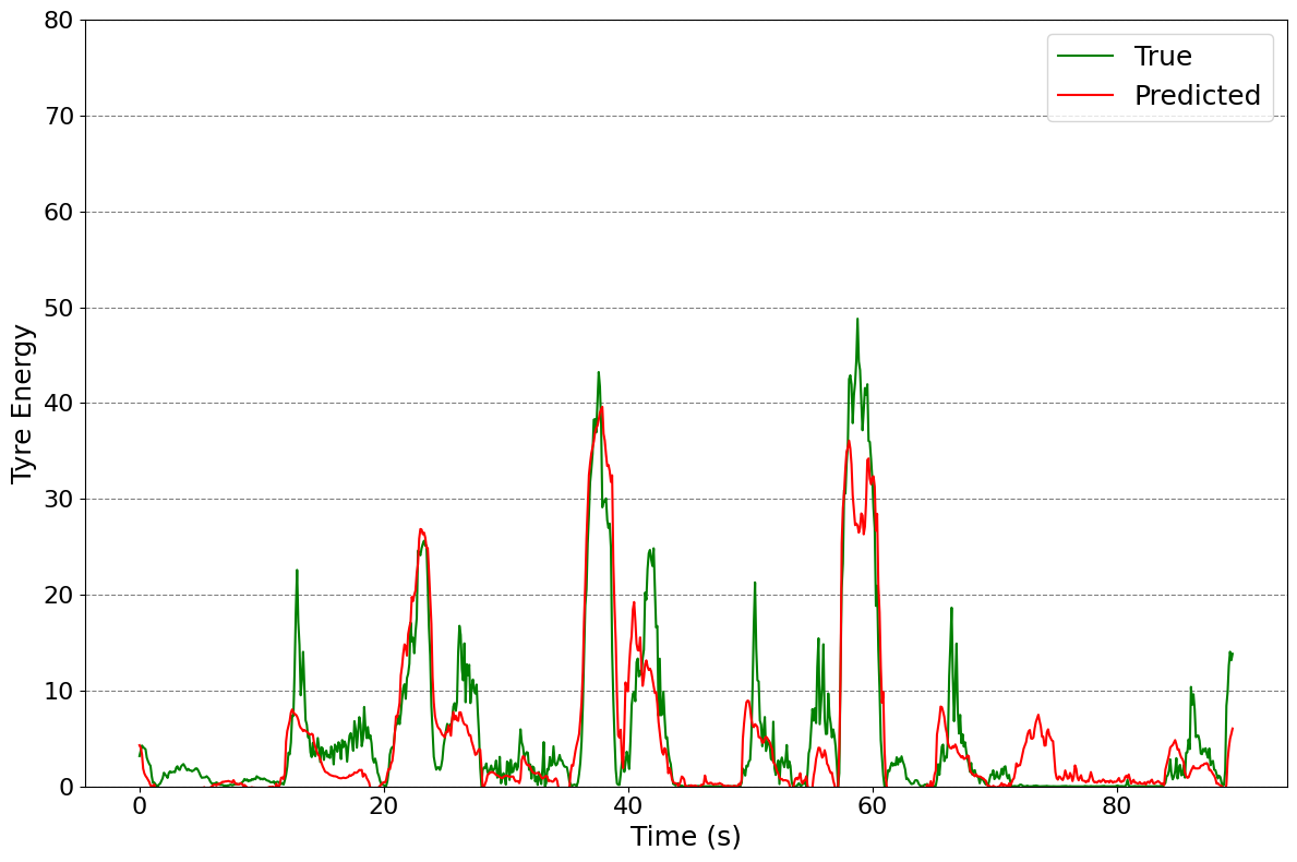
Figure 1. Green-flag XGBoost (left) and TFT (right) front-left tyre energy forecasts for one lap of a seen open track

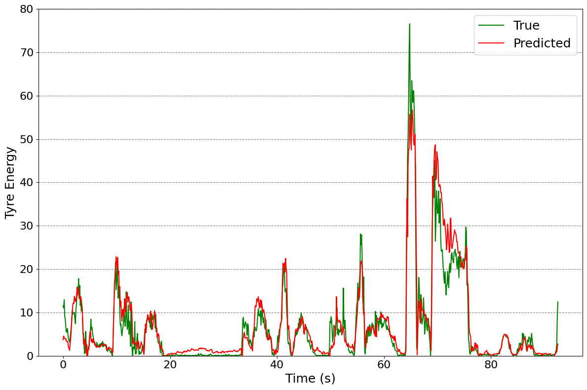
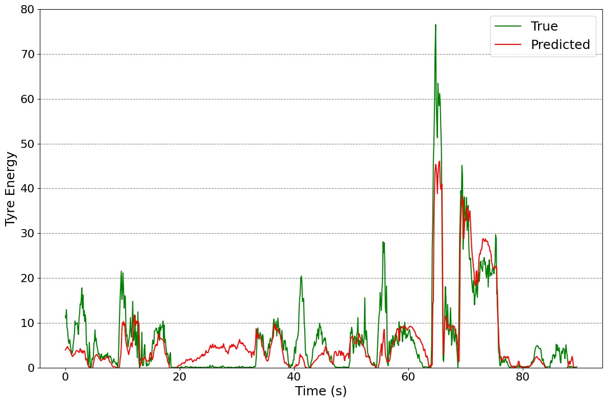
Figure 2. Green-flag XGBoost (left) and TFT (right) front-right tyre energy forecasts for one lap of an unseen street circuit

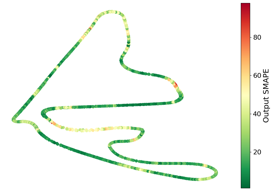
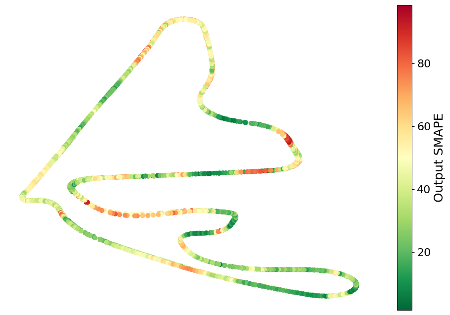
Figure 3. XGBoost (left) and TFT (right) SMAPE values over several laps of the Abu Dhabi Grand Prix (a seen open track)

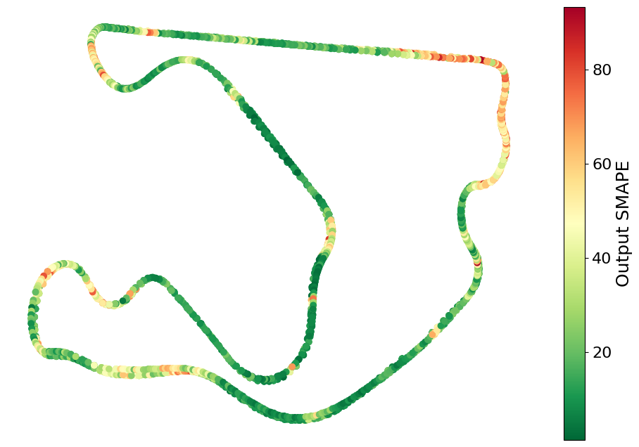
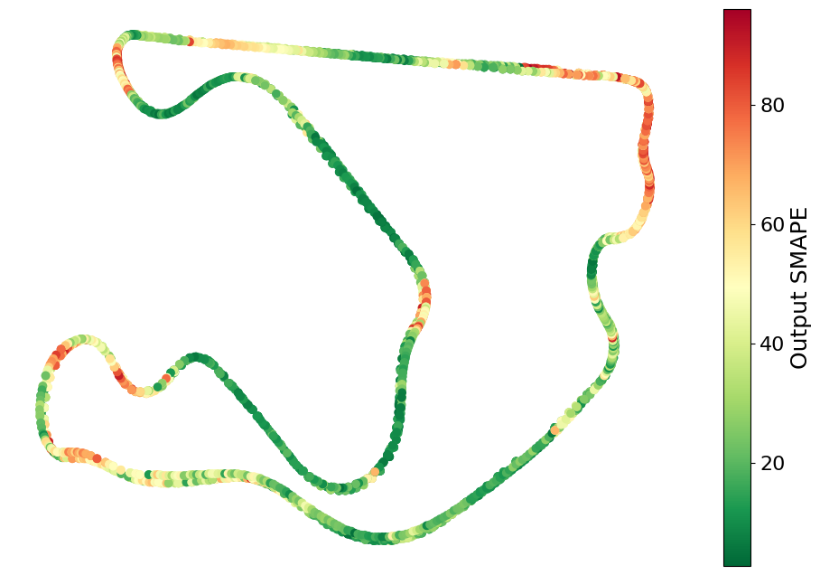
Figure 4. XGBoost (left) and TFT (right) SMAPE values over several laps of the Miami Grand Prix (an unseen street circuit)

Figure 5 details the green-flag TFT forecasts for tyres over one lap of an unseen open track. The cars follow this track clockwise, meaning it predominantly consists of right turns, and this is demonstrated by the larger energy spikes on average for the front left (compared to the front right) and rear left (compared to the rear right) tyres. This further demonstrates that our models are replicating real-world phenomena exhibited by the cars’ dynamics.

Figure 5. Green-flag TFT all tyre energy forecasts for one lap of an unseen clockwise open circuit.
The top row displays the front left and right tyres, while the bottom row displays the rear left and right tyres.

Table 3 demonstrates the results for the GRU and TFT models on seen and unseen tracks respectively. It is clear that the models perform better on seen tracks, as would be expected, but the performance difference is more obvious for the GRU models. Moreover, GRU outperforms TFT for seen races, whereas the green-flag TFT is significantly stronger for unseen events, showcasing the adaptability of the TFT.

Table 3. GRU and TFT models evaluated on several seen (Abu Dhabi, Bahrain, Austria, Monaco and Spain) and unseen (Netherlands, Qatar, Hungary, Miami and Azerbaijan) tracks, with mean results

	Seen Tracks					Seen	Unseen Tracks					Unseen
Model	Abu D.	Bahrain	Austria	Monaco	Spain	Mean	Neth.	Qatar	Hungary	Miami	Azer.	Mean
One-hot GRU	6.504	4.218	5.922	4.595	5.164	5.281	5.980	5.812	7.180	5.696	5.094	5.952
One-hot TFT	7.154	4.508	6.854	4.760	5.600	5.775	6.140	6.766	6.633	5.680	4.644	5.972
Green-flag GRU	6.393	4.279	6.257	4.753	5.472	5.431	4.817	5.949	7.102	5.500	5.309	5.735
Green-flag TFT	6.666	4.188	6.336	4.713	5.355	5.452	5.171	5.739	6.360	5.260	4.843	5.475

The TFT models were also compared against single-track specialist (STS) TFT models, which were trained on one track over multiple seasons and were evaluated on the same track for a more recent season. We speculate that, while STS models do not generalise well for arbitrary tracks, their over-fitting to the circuit would be useful in real-world applications, e.g. for planning the race strategy for a single upcoming race. Table 4 demonstrates that STS models tend to improve upon more generalised models for their specialised track, supporting this hypothesis. Monaco is an exception to this, but unlike the other evaluated tracks, the STS model trained on a single Monaco race only, which suggests that the issue here may have been a lack of data. It should also be noted that Monaco has the lowest tyre degradation, and thus tyre energies, of all tracks, and is often regarded as an exception.

Table 4. TFT models compared against STS TFT models for three distinct tracks, as well as the mean

Model	Abu D.	Austria	Monaco	Mean
One-hot TFT	7.154	6.854	4.760	6.256
Green-flag TFT	6.666	6.336	4.713	5.905
STS One-hot TFT	5.535	4.849	5.115	5.166
STS Green-flag TFT	5.834	5.300	5.269	5.468

Table 5. Forecasting TFT compared against Regression TFTs for Green-flag and Exclude encodings

Model	Azer.	Spain	Miami	Neth.	Test Set
For. G TFT	4.843	5.355	5.260	5.171	5.305
Reg. E TFT	4.572	6.163	6.131	5.393	5.558
Reg. G TFT	4.676	6.183	6.034	5.229	5.877

As a final investigation, regression-based TFT models were trained and evaluated on the complete test set as well as individual tracks. This was to test the hypothesis that 100 time steps of covariate data may be too much information for the models and thus harm the performance. These regression-based models only received one time step of covariate data and must predict the tyre energies for that same time step. From the results in Table 5, we found the TFT to be more accurate than its regression-based counterpart, although the difference in performance was not significant given the large disparity in input data size.

4.2. Explainable AI

Figure 6 ranks the feature importance of the observed covariates for the green-flag TFT, taken from its in-built interpretability module. SteeringWheelAngle, which affects how sharply the car takes corners, is the most important variable for forecasting tyre energies. Overall, the ranking of the variables is logical and is along the lines of what we were expecting, with the most relevant covariates having greater significance. For example, PitStop, which signifies whether a pit stop is taking place, is the second most important variable. This is intuitive as a car is stationary during a pit stop and thus no energy is applied to the tyres.

Figure 6. In-built TFT feature importance

TIME (Sood and Craven, 2022) produces a heat map as shown in Figure 7, which displays the temporal feature importance for the generalised TFT model. This heat map covers a ten-second window of a corner turn, including the entrance, apex and exit. Covariates corresponding to the car speed, steering wheel angle and steering coefficient are assigned high importance for the model. Steering wheel angle is only considered significant when the car starts turning; similarly, car speed is only relevant after the apex when the car starts to accelerate. This is in line with expectations, with other models producing similar results (see Figure 8).

Figure 7. TIME heat map of green-flag TFT for Miami, front-left tyre

Figure 8. TIME heat map of one-hot STS for Abu Dhabi, front-left tyre

CausalImpact (Brodersen et al., 2015) was utilised to analyse the impact of an incident during a race which led to the virtual safety car being deployed. The results are demonstrated in Figure 9. The counterfactual is the hypothetical scenario where the virtual safety car was not deployed i.e., if the race continued under green-flag conditions. The grey shaded area represents the 95% confidence interval, which is wide given the volatility of the tyre energies. The true energies were very low during this period, but the predictions reflect a typical lap. Thus, the difference is almost always negative and the cumulative impact decreases rapidly. The algorithm also calculates the probability of causal effect at 57.5%. This demonstrates that the virtual safety car had a significant impact on reducing the tyre energies during its active period.

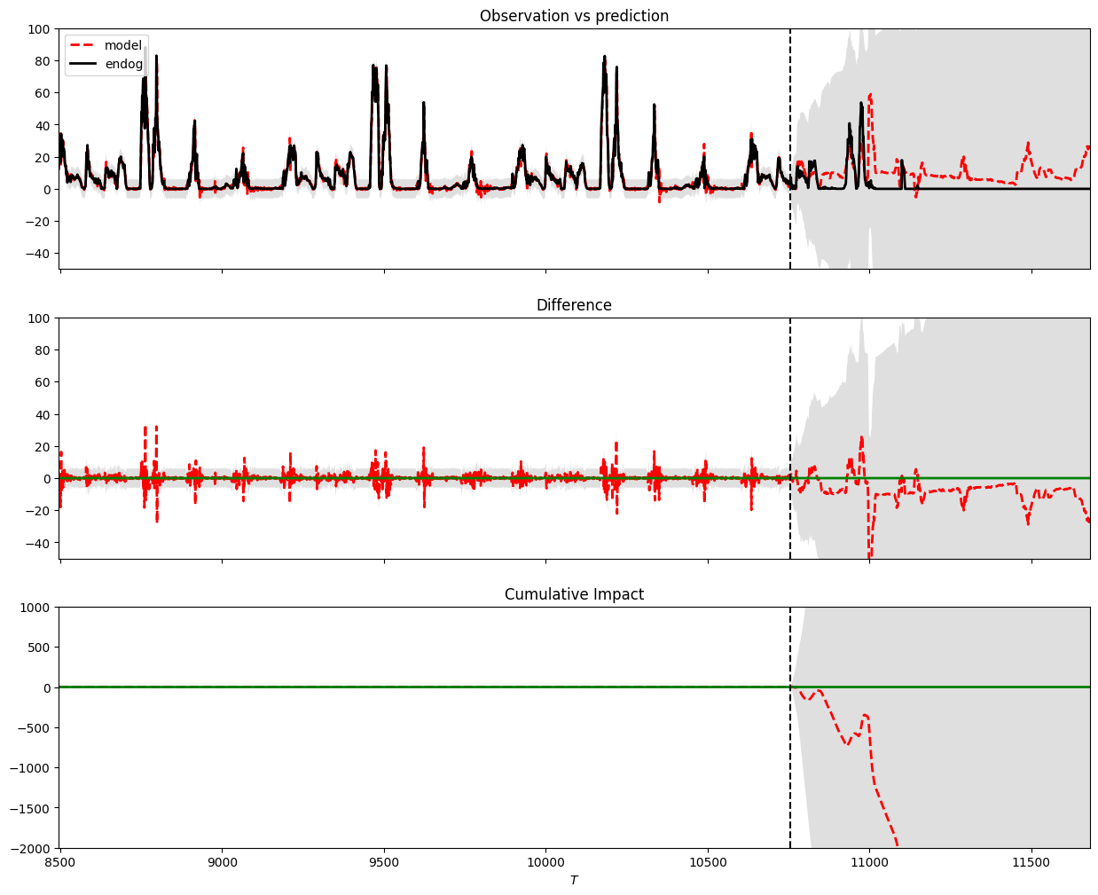
Figure 9. Causal impact of front-left tyre energies for a virtual safety car incident. The first graph gives the counterfactual predictions if the virtual safety car was not deployed (red dashed line), compared to the ground truth observations (black solid line). The second plot displays the difference between the two and the third demonstrates the cumulative difference.

5. Conclusions and Future Work

In this work, we implemented and trained three different recurrent neural network models, and integrated a state-of-the-art transformer model, to forecast tyre energies given only past covariate data. While all of these models vastly outperformed the linear regression baseline, XGBoost proved to be a very powerful tool for this particular time series forecasting task, albeit with its weaknesses such as high memory requirements and rigid training time. Despite this, we found alternative methods to improve model accuracy, such as specialising models to particular tracks. Furthermore, we incorporated XAI techniques to justify the models’ predictions.

Future work will be focused on extending the models’ capabilities to handle practice and qualifying session data to boost accuracy, as well as reconsidering which covariates could be added or removed to improve performance. More explainability methods could be utilised and assessed alongside those we have introduced here, both empirically with datasets and in user studies with race strategists to determine their effectiveness along typical XAI properties such as faithfulness (Jacovi and Goldberg, 2020), i.e. how closely the explanations replicate the models, and trust (Jacovi et al., 2021), i.e. how much users are willing to trust the model. The real-world use of our models is currently limited to post-race analysis due to their iterative processing of complete race data. Enhancing our models to process real-time data and compute predictions on the fly will extend their use to live races, potentially giving F1 teams an edge over their competitors. Finally, we would like to investigate how our models translate to the wider automotive industry, given the increasing importance of tyre degradation for air pollution as electric vehicles become widespread (Katsikouli et al., 2020).

References

- (1)
- Akiba et al. (2019) Takuya Akiba, Shotaro Sano, Toshihiko Yanase, Takeru Ohta, and Masanori Koyama. 2019. Optuna: A Next-generation Hyperparameter Optimization Framework. In KDD. 2623–2631. https://doi.org/10.1145/3292500.3330701
- Bhatt et al. (2020) Umang Bhatt, Alice Xiang, Shubham Sharma, Adrian Weller, Ankur Taly, Yunhan Jia, Joydeep Ghosh, Ruchir Puri, José M. F. Moura, and Peter Eckersley. 2020. Explainable machine learning in deployment. In FAT*. 648–657. https://doi.org/10.1145/3351095.3375624
- Bodria et al. (2023) Francesco Bodria, Fosca Giannotti, Riccardo Guidotti, Francesca Naretto, Dino Pedreschi, and Salvatore Rinzivillo. 2023. Benchmarking and survey of explanation methods for black box models. Data Min. Knowl. Discov. 37, 5 (2023), 1719–1778. https://doi.org/10.1007/S10618-023-00933-9
- Brodersen et al. (2015) Kay H. Brodersen, Fabian Gallusser, Jim Koehler, Nicolas Remy, and Steven L. Scott. 2015. Inferring causal impact using Bayesian structural time-series models. The Annals of Applied Statistics 9, 1 (2015). https://doi.org/10.1214/14-aoas788
- Chen and Guestrin (2016) Tianqi Chen and Carlos Guestrin. 2016. XGBoost: A Scalable Tree Boosting System. In KDD. 785–794. https://doi.org/10.1145/2939672.2939785
- Cho et al. (2014) Kyunghyun Cho, Bart van Merrienboer, Çaglar Gülçehre, Dzmitry Bahdanau, Fethi Bougares, Holger Schwenk, and Yoshua Bengio. 2014. Learning Phrase Representations using RNN Encoder-Decoder for Statistical Machine Translation. In EMNLP. 1724–1734. https://doi.org/10.3115/V1/D14-1179
- Ekambaram et al. (2023) Vijay Ekambaram, Arindam Jati, Nam Nguyen, Phanwadee Sinthong, and Jayant Kalagnanam. 2023. TSMixer: Lightweight MLP-Mixer Model for Multivariate Time Series Forecasting. In KDD. 459–469. https://doi.org/10.1145/3580305.3599533
- Hochreiter and Schmidhuber (1997) Sepp Hochreiter and Jürgen Schmidhuber. 1997. Long Short-Term Memory. Neural Comput. 9, 8 (1997), 1735–1780. https://doi.org/10.1162/NECO.1997.9.8.1735
- Jacovi and Goldberg (2020) Alon Jacovi and Yoav Goldberg. 2020. Towards Faithfully Interpretable NLP Systems: How Should We Define and Evaluate Faithfulness?. In ACL. 4198–4205. https://doi.org/10.18653/V1/2020.ACL-MAIN.386
- Jacovi et al. (2021) Alon Jacovi, Ana Marasovic, Tim Miller, and Yoav Goldberg. 2021. Formalizing Trust in Artificial Intelligence: Prerequisites, Causes and Goals of Human Trust in AI. In FAccT. 624–635. https://doi.org/10.1145/3442188.3445923
- Kamolthip (2021) Sarun Kamolthip. 2021. Macroeconomic forecasting with LSTM and mixed frequency time series data. CoRR abs/2109.13777 (2021). arXiv:2109.13777 https://arxiv.org/abs/2109.13777
- Katsikouli et al. (2020) Panagiota Katsikouli, Pietro Ferraro, Hugo Richardson, Hanson Cheng, Siobhan Anderson, Deepak Mallya, David Timoney, Marc Masen, and Robert Shorten. 2020. Distributed Ledger Enabled Control of Tyre Induced Particulate Matter in Smart Cities. Frontiers in Sustainable Cities 2 (2020). https://doi.org/10.3389/frsc.2020.575482
- Kim et al. (2023) Kangjun Kim, Hyunjae Park, and Taewung Kim. 2023. Comparison of Performance of Predicting the Wear Amount of Tire Tread Depending on Sensing Information. Sensors 23, 1 (2023), 459. https://doi.org/10.3390/S23010459
- Kingma and Welling (2014) Diederik P. Kingma and Max Welling. 2014. Auto-Encoding Variational Bayes. In ICLR. http://arxiv.org/abs/1312.6114
- Lim et al. (2019) Bryan Lim, Sercan Ömer Arik, Nicolas Loeff, and Tomas Pfister. 2019. Temporal Fusion Transformers for Interpretable Multi-horizon Time Series Forecasting. CoRR abs/1912.09363 (2019). arXiv:1912.09363 http://arxiv.org/abs/1912.09363
- Nie et al. (2023) Yuqi Nie, Nam H. Nguyen, Phanwadee Sinthong, and Jayant Kalagnanam. 2023. A Time Series is Worth 64 Words: Long-term Forecasting with Transformers. In ICLR. https://openreview.net/pdf?id=Jbdc0vTOcol
- Rojat et al. (2021) Thomas Rojat, Raphaël Puget, David Filliat, Javier Del Ser, Rodolphe Gelin, and Natalia Díaz Rodríguez. 2021. Explainable Artificial Intelligence (XAI) on TimeSeries Data: A Survey. CoRR abs/2104.00950 (2021). arXiv:2104.00950 https://arxiv.org/abs/2104.00950
- Rumelhart et al. (1986) D. E. Rumelhart, G. E. Hinton, and R. J. Williams. 1986. Learning Internal Representations by Error Propagation. MIT Press, Cambridge, MA, USA, 318–362.
- Salinas et al. (2017) David Salinas, Valentin Flunkert, and Jan Gasthaus. 2017. DeepAR: Probabilistic Forecasting with Autoregressive Recurrent Networks. CoRR abs/1704.04110 (2017). arXiv:1704.04110 http://arxiv.org/abs/1704.04110
- Schockaert et al. (2020) Cedric Schockaert, Reinhard Leperlier, and Assaad Moawad. 2020. Attention Mechanism for Multivariate Time Series Recurrent Model Interpretability Applied to the Ironmaking Industry. CoRR abs/2007.12617 (2020). arXiv:2007.12617 https://arxiv.org/abs/2007.12617
- Sood and Craven (2022) Akshay Sood and Mark Craven. 2022. Feature Importance Explanations for Temporal Black-Box Models. In AAAI. 8351–8360. https://doi.org/10.1609/AAAI.V36I8.20810
- Vaswani et al. (2017) Ashish Vaswani, Noam Shazeer, Niki Parmar, Jakob Uszkoreit, Llion Jones, Aidan N. Gomez, Lukasz Kaiser, and Illia Polosukhin. 2017. Attention is All you Need. In NeurIPS. 5998–6008. https://proceedings.neurips.cc/paper/2017/hash/3f5ee243547dee91fbd053c1c4a845aa-Abstract.html
- von Schleinitz et al. (2021) Julian von Schleinitz, Michael Graf, Wolfgang Trutschnig, and Andreas Schröder. 2021. VASP: An autoencoder-based approach for multivariate anomaly detection and robust time series prediction with application in motorsport. Eng. Appl. Artif. Intell. 104 (2021), 104354. https://doi.org/10.1016/J.ENGAPPAI.2021.104354
- Zeng et al. (2023) Ailing Zeng, Muxi Chen, Lei Zhang, and Qiang Xu. 2023. Are Transformers Effective for Time Series Forecasting?. In AAAI. 11121–11128. https://doi.org/10.1609/AAAI.V37I9.26317
- Zhang et al. (2020) Haomeng Zhang, Shiwen Zhang, Yue Zhang, Xiaojing Huang, and Yi Dai. 2020. Abrasion Status Prediction with BP Neural Network Based on an Intelligent Tire System. In CVCI.