Hermitian and Non-Hermitian Topological Transitions Characterized by Manifold Distance
Abstract
Topological phases are generally characterized by topological invariants denoted by integer numbers. However, different topological systems often require diffenent topological invariants to measure, and theses definition usually fail at critical points. Therefore, it’s challenging to predict what would occur during the transformation between two different topological phases. To address these issues, we propose a general definition based on fidelity and trace distance from quantum information theory: manifold distance (MD). This definition does not rely on the berry connection but rather on the information of the two manifolds - their ground state wave functions. Thus, it can measure different topological systems (including traditional band topology models, non-Hermitian systems, and gapless systems, etc.) and exhibit some universal laws during the transformation between two topological phases. Our research demonstrates: for different topological manifolds, the change rate (first-order derivative) or susceptibility (second-order derivative) of MD exhibit various divergent behaviors near the critical points. Compared to the strange correlator, which could be used as a diagnosis for short-range entangled states in 1D and 2D, MD is more universal and could be applied to non-Hermitian systems and long-range entangled states. For subsequent studies, we expect the method to be generalized te real-space or non-lattice models, in order to facilitate the study of a wider range of physical platforms such as open systems and many-body localization.
In the literature of topology and geometry, two manifolds are topologically equivalent when and only when they can be smoothly deformed to each other Lee (2010). The equivalent manifolds are uniformly characterized by one topological index (invariant), such as the Chern number Lee (2010) corresponding to the famous Thouless-Kohmoto-Nightingale-den Nijs (TKNN) number derived from the linear response theory in the theory of topological matters Hatsugai (1993); Kane and Mele (2005). This pioneering breakthrough propelled the establishment of the topological classification of matters with various symmetries in all dimensions Qi and Zhang (2011); Hasan and Moore (2011); Qi and Zhang (2011); Schnyder et al. (2009, 2008). Regardless of the Hermiticity of the topological matters, theoretical explorations of non-Hermitian quantum systems have significantly expanded the scope of condensed matter physics in the past decade Ashida et al. (2020); Bergholtz et al. (2021); Gong et al. (2018); Kawabata et al. (2019a); Shen et al. (2018); Yao and Wang (2018); Song et al. (2019); Lieu (2018); Bagarello et al. (2016); Lee (2016); Kunst et al. (2018); Yao et al. (2018); Lee and Thomale (2019); Yokomizo and Murakami (2019); Okuma et al. (2020); Borgnia et al. (2020); Yang et al. (2020a); Zhang et al. (2020a); Xue et al. (2021); Guo et al. (2021); Xue et al. (2022); Fu and Zhang (2023a), rapidly encompassing higher-order non-Hermitian systems Liu et al. (2019); Lee et al. (2019); Edvardsson et al. (2019); Kawabata et al. (2020); Okugawa et al. (2020); Fu et al. (2021); Yu et al. (2021); Palacios et al. (2021); Li et al. (2022), exceptional points Kawabata et al. (2019b); Yokomizo and Murakami (2020); Yang et al. (2020b); Zhang et al. (2020b); Xue et al. (2020); Yang et al. (2021); Denner et al. (2021); Fu and Wan (2022); Mandal and Bergholtz (2021); Delplace et al. (2021); Liu et al. (2021); Stålhammar and Bergholtz (2021); Ghorashi et al. (2021a, b), and scale-free localization Li et al. (2021, 2023); Guo et al. (2023); Fu and Zhang (2023b); Molignini et al. (2023). In open boundary conditions (OBSs), the non-Hermitian skin effect (NHSE) is a remarkable feature that predicts an extensive number of eigenstates localized at the edges as well as the breakdown of the Bloch band theory Lee (2016); Yao and Wang (2018); Song et al. (2019); Yokomizo and Murakami (2019); Zhang et al. (2020a); Yang et al. (2020a); Okuma et al. (2020). A comprehensive consequence is the difference of the topological transition points between OBCs and periodic boundary conditions (PBCs).
However, a subtle question has never been addressed in either Hermitian or non-Hermitian systems: what quantitative contexts will happen during the deformation of the transition of two manifolds (topological phases)? Note that in quantum information science, there are two common ways to measure the similarity between two pieces of information: trace distance and fidelity (in the case of pure states, these are completely equivalent) Jozsa (1994); Nandi et al. (2018); Liang et al. (2019); Gu (2010); Banchi et al. (2015); Li (2012); Rastegin (2007, 2007); Zhang et al. (2019); de Miranda and Micklitz (2023); Liang et al. (2019); Brito et al. (2018); Rana et al. (2016). Based on this concept, various new definitions emerge for different physical systems, such as the fidelity rate to characterize the quantum phase transition of the ground state Gu (2010); Banchi et al. (2015), the trace distance quantum discord to measure the quantum correlation Rana et al. (2016), and the minimum trace distance to quantify the non-locality of Bell-type inequalities Brito et al. (2018). These generalized concepts are built upon the significant distinctions in “distances” between different phases of matter. Thus, the measurement of the quantum state serves as an inspiration for our investigation of the topological phase boundaries Wiseman and Milburn (2009); Zeng et al. (2019).
In this work, we establish a formulation to analyze the divergent behavior observed during the deformation of two manifolds representing topological phases. We introduce the concept of “manifold distance (MD)” as a tool for efficiently and directly identifying the boundaries of topological phases. We find that MD, along with its higher-order derivatives, transitions smoothly between two topologically equivalent manifolds (phases). However, at critical points separating distinct topological phases, the higher-order derivatives of MD exhibit distinct divergent behaviors governed by universal scaling laws.
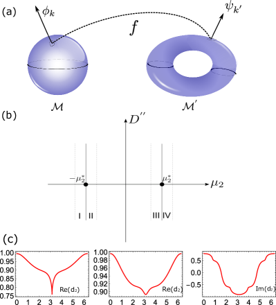
Our MD formulation is broadly applicable, extending not only to conventional Hermitian systems but also to non-Hermitian systems under both open boundary conditions (OBCs) and periodic boundary conditions (PBCs). Furthermore, we demonstrate the applicability of our method to (many-body) continuous systems, including -wave superconductors and the Kitaev toric code model, which exhibits topological order. This approach provides a rigorous means to characterize and understand the behavior at topological phase boundaries. A pictorial representation of this process is shown in Fig. 1.
To illustrate the formulation, consider two manifolds, and , whose parameters are mapped onto each other via a smooth function:
| (1) |
The mapping functions, which quantify the distance between different ground-state wavefunctions, exhibit divergent behavior at the critical points of phase transitions.
Manifold distance.- The most natural definition of manifold distance is based on the trace distanceJozsa (1994), which, for pure states, is exactly equivalent to fidelity Jozsa (1994); Liang et al. (2019). We define two distinct distance measures as follows:
| (2) |
It is evident that and .
Our primary focus is on pure states, although the same definitions could be extended to mixed states. In such cases, the overlap between two distinct regions is determined by the distance between the corresponding density matrices Jozsa (1994). To quantify the distance between two manifolds, we define the manifold distances as:
| (3) |
A distance implies that, for every and , the two wavefunctions are identical.
The concept of manifold distance can be intuitively understood as follows: Consider the transformation , representing a mapping within the same manifold, as illustrated in Fig. 1(d). For , we find that , where defines the Berry connection. In this case, the distances are given by:
| (4) |
If is purely imaginary, a similar calculation yields and .
During a topological phase transition, the energy bands of the system can undergo significant changes at certain points in the Brillouin zone, resulting in a divergence in the manifold distance. To illustrate these properties, we examined a simplified non-Hermitian Hamiltonian. A detailed theoretical analysis is provided in Appendix VII Sup .
In comparison to the strange correlator—an established diagnostic tool for short-range entangled states in 1D and 2D systems Shankar and Vishwanath (2011); You et al. (2014a); Wierschem and Sengupta (2014); Lepori et al. (2023); You et al. (2014b)—manifold distance is more universal. It applied to non-Hermitian systems, long-range entangled states (as demonstrated in Fig. 4), and even higher-dimensional or higher-order topological systems (results forthcoming).
Generalized to the Non-Hermitian.-Non-Hermiticity is typically introduced by incorporating non-Hermitian (NH) hopping terms and/or NH gain/loss terms Moiseyev (2011); Liu et al. (2020); Ashida et al. (2020); Bagarello et al. (2016); Kawabata et al. (2019a). Furthermore, certain topological invariants of Hermitian Hamiltonians are generalized when the Hermiticity condition is relaxed Bergholtz et al. (2021); Gong et al. (2018); Shen et al. (2018); Yao and Wang (2018); Song et al. (2019); Lieu (2018). Consequently, extending the concept of manifold distance to non-Hermitian systems is a natural progression.
Consider the eigenvalue equations of Non-Hermitian Hamiltonian :
| (5) |
Here we have four choices
| (6) |
where and correspond to and , respectively.
Thus, irrespective of the specific definition of manifold distance, the behavior of the phase boundary is effectively captured, with differences manifesting only in the numerical values.
In the context of non-Hermitian systems, it is advisabled to employ forms such as or to address normalization issues.
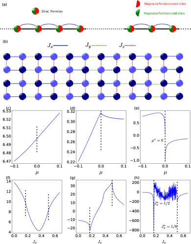
Hamiltonians.- We investigated the divergent properties of phase boundaries using one-dimensional and two-dimensional topological models Kitaev (2001); Greiter et al. (2014); Leijnse and Flensberg (2012); Günter et al. (2005); Leijnse and Flensberg (2012); Greiter et al. (2014); Chhajed (2020); Thakurathi et al. (2014); Sato and Fujimoto (2016); Ren et al. (2016). The Hamiltonians considered are as follows:
| (7) |
In case of , we define and . For , we set and , where represents the chemical potential, denotes the hopping amplitude between neighboring sites, could be interpreted as the spin-orbit coupling or superconducting pairing strength, and represents the non-Hermitian term coefficient.
These two models are representative of various topological phases. For instance, can be interpreted as the Kitaev toy model. Similarly, could be associated with a two-dimensional superconducting model.
Let us first analyzed the Hamiltonian . We assume that the parameters for the manifold are , and , while for the corresponding manifold , the parameters are , and . Based on the expression for , we found that singular points occur at when , or at when . Similarly, for the Hamiltonian , the singular points are located at .
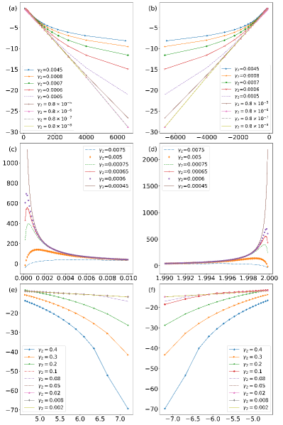
Transition from non-Hermitian to Hermitian.- As for the above Non-Hermitian Hamiltonian and , when , they both reback to Hermitian systems. This transition phenomenon can be demonstrated using the manifold distance. For instance, the divergence behavior of at the phase boundary would reverts from non-Hermitian to Hermitian systems, as shown in Fig. (2).
For the Non-Hermitian Hamiltonians and discussed above, as , both systems reduce to their Hermitian systems. This transition could be effectively characterized using the manifold distance. Specifically, the divergence behavior of at the phase boundary transitions from the non-Hermitian regime to the Hermitian regime, as illustrated in Fig. (2).
Consider a simplified 1D Hamiltonian:
| (10) |
Numerical calculations revealed that the divergence coefficients are primarily influenced by a specific set of parameters. For simplicity, we assumed the first set of parameters to be constants and omit the subscripts in subsequent discussions. Since the simplified Hamiltonian lacks a Brillouin zone, we only need to consider integration intervals that encompass the singularities of , where denotes the partial derivative of with respect to the chemical potential. When the non-Hermitian term is large , the divergence behavior of is approximately given by:
| (11) |
As for , the divergence behavior transitions to:
| (12) |
which corresponds to the behavior of a Hermitian system. This result shows that as the non-Hermitian term gradually vanishes, the divergence behavior transitions from to , with a superposition of divergence behaviors observed during this process. Coefficients for additional models could be found in Section IX of the supplementary materials Sup .
Finally, although the divergence behavior of () is affected by several parameters, its divergence coefficient tends to depend on only a few physical parameters for Hermitian case.
For the Hermitian model defined in eq. 7, our numerical fitting confirm that
| (13) |
For non-Hermitian systems, the divergence behavior is as follows:
| (14) | |||
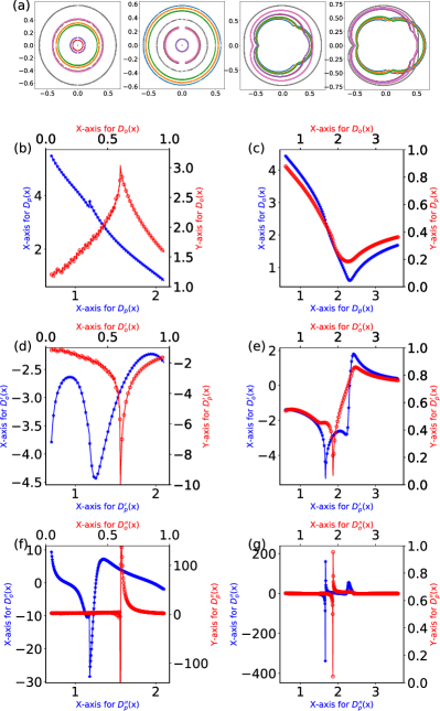
Open boundary for non-Hermitian systems.- The bulk-boundary correspondence, which was originally developed for Hermitian systems. However, for non-Hermitian systems, the open-boundary spectrum significantly differs from the periodic boundary case. Specifically, the momentum-space Hamiltonian may fail to fully determine the zero modes. In general, the zero modes or phase boundaries could be observed in the numerical spectra of the real-space Hamiltonian with open boundaries. In this context, we proposed a universally applicable approach that directly employs manifold distance to determined phase boundaries in momentum space. As a specific illustrative example, we consider the 1D PT-symmetric non-Hermitian Su-Schrieffer-Heeger (SSH) model Yao and Wang (2018).
| (17) |
with
| (18) | |||
We show a shortcut, which is applicable only to the case. For PBCs, the phase critical lines are
| (19) |
and the devergence behavior as follow
| (20) |
In non-Hermitian systems, the open-boundary spectra quite different from periodic-boundary ones, which seems to indicate a complete breakdown of bulk-boundary correspondence, and its transition points
| (21) |
Nevertheless, the derivative of maifold distance can also manifest the phase transition, whether the system has PBC or OBC, as show in fig.3. However, for OBC, some modifications are necessary for manifold distance.
i) The integration region for manifold distance should be the generalized Brillouin zone; more precisely, it should include the ”singularities” of GBZ;
ii) Correspondingly, it is necessary to extended the momentum to its complex form, i.e.,
| (22) |
which is equivalent to replacing the Bloch phase factor by in OBC.
Similarly, for systems with next-nearest neighbors, we could consider the phase boundary, as shown in Fig. 3. While an analytical expression for the phase boundary is not available, it could be numerically obtained through the singularities of the manifold distance.
In fact, for non-lattice systems, it is necessary to truncate the integration domain, as long as these ”singular points” are contained within it. In this way, its derivatives also exhibit divergence properties near phase boundary, such as p-wave superconductor model shown in fig.4. Even for topological order systems with long-range entangled states, our manifold distance approach remains effective, as demonstrated in Fig. 4.
To conclude, we have defined the manifold distance over two manifolds and shown that its higher-order derivatives can exhibit scaling laws at the critical points when crossing the topological phase boundary. We have identified some divergence behaviors in one- and two-dimensional models and have demonstrated that this approach can be extended to non-Hermitian systems with open boundary conditions (OBCs).
For future research, we plan to extend this concept to mixed states and apply it to open systems to investigate the effects of gain and loss on various experimental platforms. Specifically, we aim to study the manifold distance given by . We expect to obtain similar results for open systems. Furthermore, we aim to generalize these definitions to broader domains, such as real space or quasi-crystal systems.
Acknowledgments.- This work is supported by …
References
- Lee (2010) J. Lee, Introduction to topological manifolds, Vol. 202 (Springer Science & Business Media, 2010).
- Hatsugai (1993) Y. Hatsugai, Physical review letters 71, 3697 (1993).
- Kane and Mele (2005) C. L. Kane and E. J. Mele, Physical review letters 95, 146802 (2005).
- Qi and Zhang (2011) X.-L. Qi and S.-C. Zhang, Reviews of Modern Physics 83, 1057 (2011).
- Hasan and Moore (2011) M. Z. Hasan and J. E. Moore, Annu. Rev. Condens. Matter Phys. 2, 55 (2011).
- Schnyder et al. (2009) A. P. Schnyder, S. Ryu, A. Furusaki, and A. W. Ludwig, in AIP Conference Proceedings, Vol. 1134 (American Institute of Physics, 2009) pp. 10–21.
- Schnyder et al. (2008) A. P. Schnyder, S. Ryu, A. Furusaki, and A. W. Ludwig, Physical Review B 78, 195125 (2008).
- Ashida et al. (2020) Y. Ashida, Z. Gong, and M. Ueda, Advances in Physics 69, 249 (2020).
- Bergholtz et al. (2021) E. J. Bergholtz, J. C. Budich, and F. K. Kunst, Reviews of Modern Physics 93, 015005 (2021).
- Gong et al. (2018) Z. Gong, Y. Ashida, K. Kawabata, K. Takasan, S. Higashikawa, and M. Ueda, Physical Review X 8, 031079 (2018).
- Kawabata et al. (2019a) K. Kawabata, K. Shiozaki, M. Ueda, and M. Sato, Physical Review X 9, 041015 (2019a).
- Shen et al. (2018) H. Shen, B. Zhen, and L. Fu, Physical review letters 120, 146402 (2018).
- Yao and Wang (2018) S. Yao and Z. Wang, Physical review letters 121, 086803 (2018).
- Song et al. (2019) F. Song, S. Yao, and Z. Wang, Physical review letters 123, 246801 (2019).
- Lieu (2018) S. Lieu, Physical Review B 97, 045106 (2018).
- Bagarello et al. (2016) F. Bagarello, R. Passante, C. Trapani, et al., Springer Proceedings in Physics 184 (2016).
- Lee (2016) T. E. Lee, Phys. Rev. Lett. 116, 133903 (2016).
- Kunst et al. (2018) F. K. Kunst, E. Edvardsson, J. C. Budich, and E. J. Bergholtz, Phys. Rev. Lett. 121, 026808 (2018).
- Yao et al. (2018) S. Yao, F. Song, and Z. Wang, Phys. Rev. Lett. 121, 136802 (2018).
- Lee and Thomale (2019) C. H. Lee and R. Thomale, Phys. Rev. B 99, 201103 (2019).
- Yokomizo and Murakami (2019) K. Yokomizo and S. Murakami, Phys. Rev. Lett. 123, 066404 (2019).
- Okuma et al. (2020) N. Okuma, K. Kawabata, K. Shiozaki, and M. Sato, Phys. Rev. Lett. 124, 086801 (2020).
- Borgnia et al. (2020) D. S. Borgnia, A. J. Kruchkov, and R.-J. Slager, Phys. Rev. Lett. 124, 056802 (2020).
- Yang et al. (2020a) Z. Yang, K. Zhang, C. Fang, and J. Hu, Phys. Rev. Lett. 125, 226402 (2020a).
- Zhang et al. (2020a) K. Zhang, Z. Yang, and C. Fang, Phys. Rev. Lett. 125, 126402 (2020a).
- Xue et al. (2021) W.-T. Xue, M.-R. Li, Y.-M. Hu, F. Song, and Z. Wang, Phys. Rev. B 103, L241408 (2021).
- Guo et al. (2021) C.-X. Guo, C.-H. Liu, X.-M. Zhao, Y. Liu, and S. Chen, Phys. Rev. Lett. 127, 116801 (2021).
- Xue et al. (2022) W.-T. Xue, Y.-M. Hu, F. Song, and Z. Wang, Phys. Rev. Lett. 128, 120401 (2022).
- Fu and Zhang (2023a) Y. Fu and Y. Zhang, Phys. Rev. B 107, 115412 (2023a).
- Liu et al. (2019) T. Liu, Y.-R. Zhang, Q. Ai, Z. Gong, K. Kawabata, M. Ueda, and F. Nori, Phys. Rev. Lett. 122, 076801 (2019).
- Lee et al. (2019) C. H. Lee, L. Li, and J. Gong, Phys. Rev. Lett. 123, 016805 (2019).
- Edvardsson et al. (2019) E. Edvardsson, F. K. Kunst, and E. J. Bergholtz, Phys. Rev. B 99, 081302 (2019).
- Kawabata et al. (2020) K. Kawabata, M. Sato, and K. Shiozaki, Phys. Rev. B 102, 205118 (2020).
- Okugawa et al. (2020) R. Okugawa, R. Takahashi, and K. Yokomizo, Phys. Rev. B 102, 241202 (2020).
- Fu et al. (2021) Y. Fu, J. Hu, and S. Wan, Phys. Rev. B 103, 045420 (2021).
- Yu et al. (2021) Y. Yu, M. Jung, and G. Shvets, Phys. Rev. B 103, L041102 (2021).
- Palacios et al. (2021) L. S. Palacios, S. Tchoumakov, M. Guix, I. Pagonabarraga, S. Sánchez, and A. G. Grushin, Nature Communications 12, 4691 (2021).
- Li et al. (2022) Y. Li, C. Liang, C. Wang, C. Lu, and Y.-C. Liu, Phys. Rev. Lett. 128, 223903 (2022).
- Kawabata et al. (2019b) K. Kawabata, T. Bessho, and M. Sato, Phys. Rev. Lett. 123, 066405 (2019b).
- Yokomizo and Murakami (2020) K. Yokomizo and S. Murakami, Phys. Rev. Research 2, 043045 (2020).
- Yang et al. (2020b) Z. Yang, C.-K. Chiu, C. Fang, and J. Hu, Phys. Rev. Lett. 124, 186402 (2020b).
- Zhang et al. (2020b) Z. Zhang, Z. Yang, and J. Hu, Phys. Rev. B 102, 045412 (2020b).
- Xue et al. (2020) H. Xue, Q. Wang, B. Zhang, and Y. D. Chong, Phys. Rev. Lett. 124, 236403 (2020).
- Yang et al. (2021) Z. Yang, A. P. Schnyder, J. Hu, and C.-K. Chiu, Phys. Rev. Lett. 126, 086401 (2021).
- Denner et al. (2021) M. M. Denner, A. Skurativska, F. Schindler, M. H. Fischer, R. Thomale, T. Bzdušek, and T. Neupert, Nature Communications 12, 5681 (2021).
- Fu and Wan (2022) Y. Fu and S. Wan, Phys. Rev. B 105, 075420 (2022).
- Mandal and Bergholtz (2021) I. Mandal and E. J. Bergholtz, Phys. Rev. Lett. 127, 186601 (2021).
- Delplace et al. (2021) P. Delplace, T. Yoshida, and Y. Hatsugai, Phys. Rev. Lett. 127, 186602 (2021).
- Liu et al. (2021) T. Liu, J. J. He, Z. Yang, and F. Nori, Phys. Rev. Lett. 127, 196801 (2021).
- Stålhammar and Bergholtz (2021) M. Stålhammar and E. J. Bergholtz, Phys. Rev. B 104, L201104 (2021).
- Ghorashi et al. (2021a) S. A. A. Ghorashi, T. Li, M. Sato, and T. L. Hughes, Phys. Rev. B 104, L161116 (2021a).
- Ghorashi et al. (2021b) S. A. A. Ghorashi, T. Li, and M. Sato, Phys. Rev. B 104, L161117 (2021b).
- Li et al. (2021) L. Li, C. H. Lee, and J. Gong, Communications Physics 4, 42 (2021).
- Li et al. (2023) B. Li, H.-R. Wang, F. Song, and Z. Wang, Phys. Rev. B 108, L161409 (2023).
- Guo et al. (2023) C.-X. Guo, X. Wang, H. Hu, and S. Chen, Phys. Rev. B 107, 134121 (2023).
- Fu and Zhang (2023b) Y. Fu and Y. Zhang, Phys. Rev. B 108, 205423 (2023b).
- Molignini et al. (2023) P. Molignini, O. Arandes, and E. J. Bergholtz, Phys. Rev. Res. 5, 033058 (2023).
- Jozsa (1994) R. Jozsa, Journal of modern optics 41, 2315 (1994).
- Nandi et al. (2018) S. Nandi, C. Datta, A. Das, and P. Agrawal, The European Physical Journal D 72, 1 (2018).
- Liang et al. (2019) Y.-C. Liang, Y.-H. Yeh, P. E. Mendonça, R. Y. Teh, M. D. Reid, and P. D. Drummond, Reports on Progress in Physics 82, 076001 (2019).
- Gu (2010) S.-J. Gu, International Journal of Modern Physics B 24, 4371 (2010).
- Banchi et al. (2015) L. Banchi, S. L. Braunstein, and S. Pirandola, Physical review letters 115, 260501 (2015).
- Li (2012) Y. Li, Physics Letters A 376, 1025 (2012).
- Rastegin (2007) A. E. Rastegin, Journal of Physics A: Mathematical and Theoretical 40, 9533 (2007).
- Zhang et al. (2019) J. Zhang, P. Ruggiero, and P. Calabrese, Physical Review Letters 122, 141602 (2019).
- de Miranda and Micklitz (2023) J. T. de Miranda and T. Micklitz, Journal of Physics A: Mathematical and Theoretical 56, 175301 (2023).
- Brito et al. (2018) S. G. d. A. Brito, B. Amaral, and R. Chaves, Physical Review A 97, 022111 (2018).
- Rana et al. (2016) S. Rana, P. Parashar, and M. Lewenstein, Physical Review A 93, 012110 (2016).
- Wiseman and Milburn (2009) H. M. Wiseman and G. J. Milburn, Quantum measurement and control (Cambridge university press, 2009).
- Zeng et al. (2019) B. Zeng, X. Chen, D.-L. Zhou, X.-G. Wen, et al., Quantum information meets quantum matter (Springer, 2019).
- (71) Supplemental Material .
- Shankar and Vishwanath (2011) R. Shankar and A. Vishwanath, Physical review letters 107, 106803 (2011).
- You et al. (2014a) Y.-Z. You, Z. Bi, A. Rasmussen, K. Slagle, and C. Xu, Physical review letters 112, 247202 (2014a).
- Wierschem and Sengupta (2014) K. Wierschem and P. Sengupta, Physical Review B 90, 115157 (2014).
- Lepori et al. (2023) L. Lepori, M. Burrello, A. Trombettoni, and S. Paganelli, Physical Review B 108, 035110 (2023).
- You et al. (2014b) Y.-Z. You, Z. Wang, J. Oon, and C. Xu, Physical Review B 90, 060502 (2014b).
- Moiseyev (2011) N. Moiseyev, Non-Hermitian quantum mechanics (Cambridge University Press, 2011).
- Liu et al. (2020) S. Liu, S. Ma, C. Yang, L. Zhang, W. Gao, Y. J. Xiang, T. J. Cui, and S. Zhang, Physical Review Applied 13, 014047 (2020).
- Kitaev (2001) A. Y. Kitaev, Physics-uspekhi 44, 131 (2001).
- Greiter et al. (2014) M. Greiter, V. Schnells, and R. Thomale, Annals of Physics 351, 1026 (2014).
- Leijnse and Flensberg (2012) M. Leijnse and K. Flensberg, Semiconductor Science and Technology 27, 124003 (2012).
- Günter et al. (2005) K. Günter, T. Stöferle, H. Moritz, M. Köhl, and T. Esslinger, Physical review letters 95, 230401 (2005).
- Chhajed (2020) K. Chhajed, arXiv preprint arXiv:2009.01078 (2020).
- Thakurathi et al. (2014) M. Thakurathi, K. Sengupta, and D. Sen, Phys. Rev. B 89, 235434 (2014).
- Sato and Fujimoto (2016) M. Sato and S. Fujimoto, J. Phys. Soc. Jpn. 85, 072001 (2016).
- Ren et al. (2016) Y. Ren, Z. Qiao, and Q. Niu, Reports on Progress in Physics 79, 066501 (2016).