Stable bi-frequency spinor modes as Dark Matter candidates

Abstract

We show that bi-frequency solitary waves are generically present in fermionic systems with scalar self-interaction, such as the Dirac–Klein–Gordon system and the Soler model. We develop the approach to stability properties of such waves and use the radial reduction to show that indeed the (linear) stability is available. We conjecture that stable bi-frequency modes serve as storages of the Dark Matter.

Localized modes – or quasiparticles – are well-known in the classical field theories. These include polarons from Quantum Electrodynamics and skyrmions, topological solitons in nonlinear sigma models initially used to describe nucleons (see e.g. [1, 2]). Polarons were found related to physical phenomena such as charge transport, surface reactivity, colossal magnetoresistance, thermoelectricity, photoemission, and (multi)ferroism, and high-temperature superconductivity [3], while magnetic skyrmions, discovered in 2009 [4], are now under consideration as potential information carriers in spintronics [5]. At the same time, localized modes of classical spinor fields would always be treated with certain prejudice: the Dirac sea hypothesis, the one which prohibits electrons from descending into negative energy states, is based on the second quantization and the Pauli exclusion principle, and it would seem to fail for classical spinor fields, seemingly rendering them unstable and ready to plunge into the sea of negative energies. Yet, systems of classical spinor fields have stable modes [6, 7], which makes such models physically viable. Indeed, nonlinear Dirac equation (NLD) appears in the theory of Bose–Einstein condensates [8] and in photonics [9]. Nonlinear spinor models are discussed in the context of Quantum Gravity, Cosmology, Dark Matter, and Dark Energy [10].

There is a phenomenon intrinsic to systems of spinors with scalar self-interaction: besides “Schrödinger-type” modes

$$\psi(t,x)=\upvarphi_{0}(x)e^{-\mathrm{i}\omega t}\in\mathbb{C}^{4},\quad x\in\mathbb{R}^{3},\quad\omega\in\mathbb{R},$$ (1)

which are known to exist in the Soler model [11], such systems admit localized bi-frequency modes [12], of the form

$$\psi(t,x)=\upvarphi(x)e^{-\mathrm{i}\omega t}+\chi(x)e^{\mathrm{i}\omega t}.$$ (2)

The phenomenon of bi-frequency modes has been overlooked for years, in spite of the discovery [13] of $\mathbf{SU}(1,1)$ symmetry in the Dirac–Klein–Gordon system (DKG) and in the NLD:

$$\psi\mapsto(a+b\mathrm{i}\gamma^{2}\bm{K})\psi,\quad a,\,b\in\mathbb{C},\quad|a|^{2}-|b|^{2}=1$$ (3)

(with $\gamma^{2}$ the corresponding Dirac matrix and $\bm{K}$ the complex conjugation; we note that $\psi^{C}=\gamma^{2}\bm{K}\psi$ is the charge conjugation), which would immediately yield bi-frequency modes (2) from (1). Most interestingly, bi-frequency modes (2) are generically genuinely bi-frequency: except in spatial dimensions $\leq 2$ [12], they cannot be obtained via transformations (3), [14]; the approach to stability of bi-frequency modes was absent. Let us emphasize that it is only bi-frequency modes that can be dynamically (asymptotically) stable: a small perturbation of (1) can be a bi-frequency mode (2), which, being itself an exact solution, cannot relax to a one-frequency mode.

Nonzero Coulomb charge of a spinor field would ruin bi-frequency modes: their charge–current densities $\bar{\psi}\gamma^{\mu}\psi$ are time-dependent (unlike the scalar quantity $\bar{\psi}\psi$) and would radiate the energy to infinity via electromagnetic field. Yukawa-type interaction via $\bar{\psi}\psi$ suggests that bi-frequency modes can be considered in relation to Dark Matter theory (see e.g. [15]), which is presently in search of suitable candidates for Dark Matter particles: stable neutral bi-frequency spinor modes in the DKG system can model massive particles in the Dark Matter sector (see [16, 17, 18]), interacting with the observed matter via the “Higgs portal”. Let us mention that models of spinor-based Dark Matter are rather popular [19], particularly so the ELKO spinors [20]. We show below that classical bi-frequency modes can be arbitrarily large while retaining their stability properties, which makes them possible storages of Dark Matter.

Bi-frequency modes, interpreted as a particle-antiparticle superposition, may model neutron–antineutron oscillations $n\mbox{-}\bar{n}$ [21] as well as phenomena related to the Dark Matter, such as neutron–mirror neutron oscillations $n\mbox{-}n^{\prime}$ [22, 23, 24, 25] (with mirror neutron $n^{\prime}$ considered to be from the Dark Matter sector), neutron lifetime anomaly [26], physics of neutron stars [27], and sterile neutrino oscillations [28, 29]. All these phenomena are presently under scrutiny in High Energy Physics as it is evolving beyond the Standard Model. Stable configurations of classical (non-quantized) nonlinear spinor field can also find applications in quantum gravity [30].

Since the construction of bi-frequency modes in the DKG system and in the Soler model is the same, we concentrate on the Soler model. We point out that the DKG system turns into the Soler model in the limit of heavy Klein–Gordon bosons and large coupling constants, when the interaction term $g\phi\psi\sim g^{2}((\partial_{t}^{2}-\Delta+M^{2})^{-1}\bar{\psi}\psi)\psi$ turns into the scalar-type self-interaction $(\bar{\psi}\psi)\psi$ of the Soler model. In this limit, the shape of localized spinor modes of DKG approaches that in the Soler model; the same convergence takes place for the operators corresponding to the linearization at a localized mode and hence for the linear stability properties. The approximation of DKG system with the Soler model is justified if the mass $M_{s}$ of the spinor field is much smaller than the mass $M_{b}$ of the Klein–Gordon field and $g\sim M_{b}$.

.1 Linear stability of one-frequency spinor modes

We consider the Soler model

$$\mathrm{i}\partial_{t}\psi=-\mathrm{i}\bm{\alpha}\cdot\nabla\psi+f(\bar{\psi}\psi)\beta\psi,\quad\psi(x,t)\in\mathbb{C}^{4}.$$ (4)

The self-interaction in (4) is represented by a differentiable function $f\in\mathbb{R}$; $M_{s}:=f(0)>0$ is the mass of the spinor field. The original Soler model [31, 11] is cubic: $f(\bar{\psi}\psi)=M_{s}-\bar{\psi}\psi$. Here $\bar{\psi}=\psi^{\dagger}\beta$ is the Dirac conjugate of $\psi\in\mathbb{C}^{4}$, with $\psi^{\dagger}$ denoting Hermitian conjugate of $\psi$. The Dirac matrices are $\alpha^{j}=\begin{bmatrix}0&\sigma_{j}\\ \sigma_{j}&0\end{bmatrix}$ ($1\leq j\leq 3$, with $\sigma_{j}$ the Pauli matrices), $\beta=\begin{bmatrix}I_{2}&0\\ 0&-I_{2}\end{bmatrix}$; the Dirac $\gamma$-matrices are $\gamma^{0}=\beta$, $\gamma^{j}=\beta\alpha^{j}$. There are solutions to (4) of the form [11]

$$\upvarphi(x)e^{-\mathrm{i}\omega t},\quad\upvarphi(x)=\begin{bmatrix}v(r,\omega)\bm{\xi}\\ \mathrm{i}\sigma_{r}u(r,\omega)\bm{\xi}\end{bmatrix}e^{-\mathrm{i}\omega t},\quad r=|x|,$$ (5)

where $\sigma_{r}=r^{-1}x\cdot\sigma$, $\bm{\xi}\in\mathbb{C}^{2}$, $|\bm{\xi}|=1$; the scalar functions $v(r,\omega),\,u(r,\omega)$, are real-valued and satisfy (cf. [32, 33])

$$\omega v=\partial_{r}u+2r^{-1}u+f(v^{2}-u^{2})v,\quad\omega u=-\partial_{r}v-f(v^{2}-u^{2})u.$$

Consider a perturbation of a one-frequency solitary wave (5), $\big{(}\upvarphi(x)+\rho(t,x)\big{)}e^{-\mathrm{i}\omega t}$, $\rho(t,x)\in\mathbb{C}^{4}$, The linearization at $\upvarphi e^{-\mathrm{i}\omega t}$ – that is, the linearized equation on $\rho$ – takes the form

$$\mathrm{i}\partial_{t}\rho=\mathcal{L}\rho:=D_{0}\rho+f\beta\rho+2f^{\prime}\beta\upvarphi\mathop{\rm{R\thinspace e}}\nolimits(\bar{\upvarphi}\rho)-\omega\rho,$$ (6)

with $f=f(\bar{\upvarphi}\upvarphi)$, $f^{\prime}=f^{\prime}(\bar{\upvarphi}\upvarphi)$. Note that the operator $\mathcal{L}$ is not $\mathbb{C}$-linear because of the term $\mathop{\rm{R\thinspace e}}\nolimits(\bar{\upvarphi}\rho)$. $\mathcal{L}$ has the following invariant subspaces for $-\ell\leq m\leq\ell$:

$$\mathscr{X}_{\ell,m} =\left\{\sum\limits_{\pm}\begin{bmatrix}(a_{\pm m}+b_{\pm m}\sigma_{r}\varSigma)Y_{\ell}^{\pm m}\bm{e}_{1}\\ \mathrm{i}(\sigma_{r}p_{\pm m}+q_{\pm m}\varSigma)Y_{\ell}^{\pm m}\bm{e}_{1}\end{bmatrix}\right\},$$ (7)

$$\mathscr{Y}_{\ell} =\Biggl{\{}\begin{bmatrix}a^{\scriptscriptstyle\perp}Y_{\ell}^{-\ell}\bm{e}_{2}\\ \mathrm{i}\sigma_{r}p^{\scriptscriptstyle\perp}Y_{\ell}^{-\ell}\bm{e}_{2}\end{bmatrix}\Biggr{\}},$$ (8)

Above, $\sigma_{r}=r^{-1}x\cdot\sigma$, $\varSigma=\sigma\cdot\nabla$, and $Y_{\ell}^{m}$ are spherical harmonics of degree $\ell\geq 0$ and order $|m|\leq\ell$; $a_{0},\,a_{\pm m},\,a^{\scriptscriptstyle\perp},\,\dots$ are functions of $r$. While all the invariant spaces $\mathscr{X}_{\ell,m}$, $\mathscr{Y}_{\ell}$ are needed to represent an arbitrary perturbation of a solitary wave, $\mathscr{Y}_{\ell}$ can be discarded from future consideration: the restriction of $\mathcal{L}$ onto $\mathscr{Y}_{\ell}$ coincides with selfadjoint operator $\mathcal{L}_{0}=D_{0}+f\beta-\omega I$, hence the equation $\mathrm{i}\partial_{t}\rho=\mathcal{L}\rho$ restricted onto $\mathscr{Y}_{\ell}$ cannot lead to linear instability.

In the space $\mathscr{X}_{\ell,0}$ acting on vectors with components $\Psi=(a_{0},p_{0},b_{0},q_{0})^{T}$ depending on $t$ and $r$, the operator $\mathcal{L}_{0}(\omega)$ is represented by the matrix-valued operator

$$L_{0}(\omega,\ell)=\begin{bmatrix}f-\omega&\partial_{r}+\frac{2}{r}&0&-\frac{\ell(\ell+1)}{r^{2}}\\ -\partial_{r}&-f-\omega&-\frac{\ell(\ell+1)}{r^{2}}&0\\ 0&-1&f-\omega&\partial_{r}\\ -1&0&-\partial_{r}&-f-\omega\end{bmatrix}.$$ (9)

Since the operator $\mathcal{L}(\omega)$ is not $\mathbb{C}$-linear, one considers the $\mathbb{C}$-linear operator $\mathfrak{L}(\omega)$ such that $\begin{bmatrix}\mathcal{L}\rho\\ \bm{K}\mathcal{L}\rho\end{bmatrix}=\mathfrak{L}(\omega)\begin{bmatrix}\rho\\ \bm{K}\rho\end{bmatrix}$. Perturbations corresponding to spherical harmonics of degree $\ell$ and orders $\pm m$ are mixed: the linearized equation contains $\Psi_{\ell,m}$ and $\bm{K}\Psi_{\ell,-m}$. In the space $\mathscr{X}_{\ell,m}$, when acting on vectors $\begin{bmatrix}\Psi_{m}\\ \bm{K}\Psi_{-m}\end{bmatrix}$, with $\Psi_{m}=(a_{m},p_{m},b_{m},q_{m})^{T}$, $\mathfrak{L}(\omega)$ is represented by

$$\begin{bmatrix}L_{0}(\omega,\ell)&0\\[4.30554pt] 0&L_{0}(\omega,\ell)\end{bmatrix}+\begin{bmatrix}V&-\frac{m}{r}V&V&\frac{m}{r}V\\ 0&0&0&0\\ -\frac{m}{r}V&V&\frac{m}{r}V&V\\ 0&0&0&0\end{bmatrix},$$

$$\qquad V(r,\omega)=f^{\prime}(\bar{\upvarphi}\upvarphi)\begin{bmatrix}v^{2}&-uv\\ -uv&u^{2}\end{bmatrix},$$ (10)

with $L_{0}$ from (9) and with $v,\,u$ corresponding to the profile of the solitary wave (5). The linear stability of $\mathrm{i}\partial_{t}\rho=\mathcal{L}\rho$ reduces to studying the linear stability in each of the invariant subspaces $\mathscr{X}_{\ell,m}$, $\ell\geq 0$, $-\ell\leq m\leq\ell$, which in turn reduces to studying the spectrum of operators $\mathbf{A}_{\ell,m}$ given by

$$-\mathrm{i}\left\{\begin{bmatrix}L_{0}&0\\[4.30554pt] 0&-L_{0}\end{bmatrix}+\begin{bmatrix}V&-\frac{m}{r}V&V&\frac{m}{r}V\\ 0&0&0&0\\ -V&\frac{m}{r}V&-V&-\frac{m}{r}V\\ 0&0&0&0\end{bmatrix}\right\},$$ (11)

with $L_{0}$ from (9) and $V$ from (.1). We note that the eigenvalues of $\mathbf{A}_{\ell,\pm m}$ are mutually complex conjugate.

.2 Linear stability of bi-frequency modes

By [12], if (5) is a solitary wave solution to (4), then so is a bi-frequency solitary wave or bi-frequency mode,

$$\varPhi(t,x)=\begin{bmatrix}v(r)\bm{\xi}\\ \mathrm{i}u(r)\sigma_{r}\bm{\xi}\end{bmatrix}e^{-\mathrm{i}\omega t}+\begin{bmatrix}-\mathrm{i}u(r)\sigma_{r}\bm{\eta}\\ v(r)\bm{\eta}\end{bmatrix}e^{\mathrm{i}\omega t},$$ (12)

with $\bm{\xi},\,\bm{\eta}\in\mathbb{C}^{2}$, $\bm{\xi}^{2}-\bm{\eta}^{2}=1$. If $\bm{\xi},\,\bm{\eta}\in\mathbb{C}^{2}$ are mutually orthogonal, then bi-frequency mode (12) can be obtained from one-frequency mode (5) by application of the transformation from the symmetry group $\mathbf{SU}(1,1)$ of the Soler model (see [13, 34]), given by (3). In this case, the stability of (12) follows from the corresponding result for (5) by applying to a perturbed bi-frequency mode the symmetry transformation (3) which makes one-frequency solution from a bi-frequency one. If $\langle\bm{\xi},\bm{\eta}\rangle\neq 0$, though, then a bi-frequency solitary wave (12) can not be obtained from (5) via the action of $\mathbf{SU}(1,1)$; in this case, stability analysis of (12) does not reduce to the stability analysis of (5).

We consider a perturbation of a bi-frequency mode (12) in the form $\psi(t,x)=\varPhi(t,x)+\varrho(t,x)$, where $\varrho(t,x)$ satisfies

$$\mathrm{i}\partial_{t}\varrho=D_{0}\varrho+f(\bar{\varPhi}\varPhi)\beta\varrho+2f^{\prime}(\bar{\varPhi}\varPhi)\mathop{\rm{R\thinspace e}}\nolimits(\bar{\varPhi}\varrho)\beta\varPhi.$$ (13)

We note that for $\varPhi$ from (12), $\bar{\varPhi}\varPhi$ does not depend on time. For each $\ell\in\mathbb{N}_{0}$, the linearization (13) is invariant in the spaces formed by $\varrho_{1}(t,x)$ and $\varrho_{1}(t,x)+\varrho_{2}(t,x)$, where

$$\varrho_{1}=\sum_{m=-\ell}^{\ell}\left\{\begin{bmatrix}(a_{m}+b_{m}\sigma_{r}\varSigma)Y_{\ell}^{m}\bm{\xi}\\ \mathrm{i}(\sigma_{r}p_{m}+q_{m}\varSigma)Y_{\ell}^{m}\bm{\xi}\end{bmatrix}e^{-\mathrm{i}\omega t}+\begin{bmatrix}-\mathrm{i}(\sigma_{r}\bar{p}_{m}+\bar{q}_{m}\varSigma)Y_{\ell}^{-m}\bm{\eta}\\ (\bar{a}_{m}+\bar{b}_{m}\sigma_{r}\varSigma)Y_{\ell}^{-m}\bm{\eta}\end{bmatrix}e^{\mathrm{i}\omega t}\right\}\quad\mbox{and}\quad\varrho_{2}=\begin{bmatrix}a^{\scriptscriptstyle\perp}Y_{\ell}^{-\ell}\bm{\xi}^{\perp}\\ \mathrm{i}\sigma_{r}p^{\scriptscriptstyle\perp}Y_{\ell}^{-\ell}\bm{\xi}^{\perp}\end{bmatrix}e^{\mathrm{i}\omega t},$$ (14)

with $a_{m}$, $b_{m}$, $p_{m}$, $q_{m}$, $a^{\scriptscriptstyle\perp}$, and $p^{\scriptscriptstyle\perp}$ ($|m|\leq\ell$) complex-valued functions of $t$ and $r$ and with $\bm{\xi},\,\bm{\eta}\in\mathbb{C}^{2}$ from (12). We point out that any perturbation can be decomposed into the sum $\varrho_{1}+\varrho_{2}$ with all possible $\ell\geq 0$. The invariance in these subspaces is to be understood in the sense that there is a time-independent, $\mathbb{R}$-linear (but not $\mathbb{C}$-linear) differential operator $\mathcal{A}(x,\nabla)$ such that equation (13) for $\varrho$ is equivalent to $\partial_{t}\Psi=\mathcal{A}\Psi$, where $\Psi$ contains all of $a_{m}$, $b_{m}$, $\dots$, with $|m|\leq\ell$. (The expressions (14) are such that $\mathop{\rm{R\thinspace e}}\nolimits(\bar{\varPhi}\varrho)$ does not contain factors of $e^{\pm 2\mathrm{i}\omega t}$.) Moreover, we can assume that $\varrho_{2}=0$: if $\varrho=\varrho_{1}+\varrho_{2}$ satisfies $\lambda\varrho=\mathcal{A}\varrho$, one can deduce that $\lambda\varrho_{2}=-\mathrm{i}\mathcal{L}_{0}\varrho_{2}$, with $\mathcal{L}_{0}=D_{0}+f\beta-\omega I$ selfadjoint, so $\lambda\in\mathrm{i}\mathbb{R}$, causing no linear instability. We then have:

$$\mathop{\rm{R\thinspace e}}\nolimits(\bar{\varPhi}\varrho)={\sum}_{|m|\leq\ell}\mathop{\rm{R\thinspace e}}\nolimits\big{[}(va_{m}-up_{m})Y_{\ell}^{m}$$

$$+(vb_{m}-uq_{m})\big{(}\bm{\xi}^{\dagger}\sigma_{r}\varSigma Y_{\ell}^{m}\bm{\xi}+\bm{\eta}^{\dagger}\sigma_{r}\varSigma Y_{\ell}^{m}\bm{\eta}\big{)}\big{]}.$$ (15)

One can see from (.2) that the linear stability of one-frequency and bi-frequency modes from perturbations corresponding to spherical harmonics of degree zero (same angular structure as the solitary wave itself) is the same: $\varSigma Y_{0}^{0}=0$, hence the terms with $\bm{\xi}$ and $\bm{\eta}$-dependence drop out. We postpone the detailed analysis of (.2) for general $\bm{\xi}$ and $\bm{\eta}$ for future work, focusing on the two “endpoint” cases: when $\bm{\eta}$ is parallel to $\mathrm{i}\sigma_{2}\bm{K}\bm{\xi}$ (hence orthogonal to $\bm{\xi}$) and when $\bm{\eta}$ is parallel to $\bm{\xi}$. In the first case, one has

$$\mathop{\rm{R\thinspace e}}\nolimits\big{(}\bm{\xi}^{\dagger}\sigma_{r}\varSigma Y_{\ell}^{m}\bm{\xi}+\bm{\eta}^{\dagger}\sigma_{r}\varSigma Y_{\ell}^{m}\bm{\eta}\big{)}=|\bm{\xi}|^{-2}\mathop{\rm{R\thinspace e}}\nolimits\big{[}\bm{\xi}^{\dagger}\sigma_{r}\varSigma Y_{\ell}^{m}\bm{\xi}\big{]}$$

and then the linearized operator coincides with the linearization at a one-frequency solitary wave (corresponding to the spherical harmonic of degree $\ell$ and order $m$, with the “polarization” given by $\bm{\xi}_{0}=\bm{\xi}/|\bm{\xi}|\in\mathbb{C}^{2}$ in place of $\bm{\xi}$). Indeed, in this case the bi-frequency solitary wave can be obtained from a one-frequency solitary wave via application to (12) of an appropriate $\mathbf{SU}(1,1)$ transformation (3), hence the one-frequency and bi-frequency modes share their stability properties. (We note that if $\bm{\xi}_{0}=(1,0)^{T}$, then $\mathop{\rm{R\thinspace e}}\nolimits(\bm{\xi}_{0}^{\dagger}\sigma_{r}\varSigma Y_{\ell}^{m}\bm{\xi}_{0})=-m/r$; this is what leads to factors $m/r$ in (11).)

If instead $\bm{\xi}$ and $\bm{\eta}$ are parallel (in this case, the bi-frequency solitary wave cannot be obtained from a one-frequency solitary wave with the aid of a transformation from $\mathbf{SU}(1,1)$), then the part with $\bm{\xi}$ and $\bm{\eta}$ from (.2) takes the form

$$\bm{\xi}^{\dagger}\sigma_{r}\varSigma Y_{\ell}^{m}\bm{\xi}+\bm{\eta}^{\dagger}\sigma_{r}\varSigma Y_{\ell}^{m}\bm{\eta}=|\bm{\xi}|^{-2}(1+2\bm{\eta}^{2})\bm{\xi}^{\dagger}\sigma_{r}\varSigma Y_{\ell}^{m}\bm{\xi}.$$

Comparing the above expression to (.2) with $\bm{\eta}=0$, we conclude that the linearization at a bi-frequency mode in the invariant subspace corresponding to spherical harmonics of order $\ell$ and degrees $\pm m$ is given by the same expression (11) as for one-frequency modes, but with $(1+2\bm{\eta}^{2})m$ in place of $m$, effectively corresponding to larger values of $m$. So, if a one-frequency mode is linearly stable (with respect to perturbations in invariant subspaces corresponding to all spherical harmonics), then a corresponding bi-frequency mode is also expected to be linearly stable, at least for $|\bm{\eta}|$ small enough.

.3 Numerical results

We present the spectra of the linearization at a (one-frequency) solitary wave in invariant spaces $\mathscr{X}_{\ell,m}$ for $|m|\leq\ell\leq 3$, given by $\mathbf{A}_{\ell,m}$ from (11). For simplicity, the mass of the spinor field is taken $M_{s}=1$. Computation of the spectrum is similar to [35], but with a differentiation matrix based on rational Chebyshëv polynomials in $N=1200$ grid nodes. We only consider solitary waves with $\omega\in(0.1,1)$ since as $\omega\to 0$ the numerical accuracy deteriorates. The spectrum of $\mathbf{A}_{\ell,m}$ is symmetric with respect to the real and imaginary axes; the essential spectrum consists of $\lambda\in\mathrm{i}\mathbb{R}$, $|\lambda|\geq 1-|\omega|$. The spectral (linear) instability is due to eigenvalues with $\mathop{\rm{R\thinspace e}}\nolimits\lambda>0$.

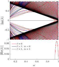
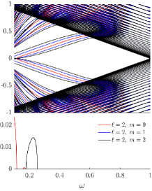
Figure 1: Imaginary (top) and real (bottom) parts of the spectrum for $\ell=0,\,1$ (left) and $\ell=2$ (right) as functions of $\omega$.

Fig. 1 (left) shows the spectrum for $\ell=0$ and $\ell=1$. (Eigenvalue $\lambda=0$ in these cases corresponds to eigenvectors $\mathrm{i}\upvarphi$ and $\partial_{x_{1}}\upvarphi$, $\partial_{x_{2}}\upvarphi$, $\partial_{x_{3}}\upvarphi$ [36].) For $\ell=0$, the instability region is $\omega\in(0.936,1)$, due to presence of a pair of real eigenvalues of opposite sign; these eigenvalues disappear via the pitchfork bifurcation when $\omega_{0}\approx 0.936$ and there are no $\mathop{\rm{R\thinspace e}}\nolimits\lambda\neq 0$ eigenvalues for $\omega<\omega_{0}$ [35]. For $\ell=1$, there are no $\mathop{\rm{R\thinspace e}}\nolimits\lambda\neq 0$ eigenvalues; eigenvalues $\lambda=\pm 2\omega\mathrm{i}$ stemming from the $\mathbf{SU}(1,1)$ symmetry [12] correspond to $|m|=\ell=1$.

For the $\ell=2$ case (right panel of Fig. 1), for $m=0$, we found a short interval of instability, $\omega\in(0.16,0.174)$, due to a quadruplet of $\mathop{\rm{R\thinspace e}}\nolimits\lambda\neq 0$ eigenvalues: this quadruplet appears and disappears at the endpoints of the interval via the Hamiltonian Hopf (HH) bifurcations, from the collisions of two pairs of purely imaginary eigenvalues. (Although the imaginary eigenvalues colliding when $\omega\approx 0.174$ are born from the same threshold, which is not in line with the Sturm–Liouville theory expectations, the form of the eigenfunctions suggests that this bifurcation is genuine, not a numerical artifact.) Next onset of instability for $|m|=0$ is from the pitchfork bifurcation at $\omega_{p}\approx 0.117$. For $|m|=1$, there is no instability; for $|m|=2$, the instability interval is $\omega\in(0.177,0.254)$, with the HH bifurcations at its endpoints.

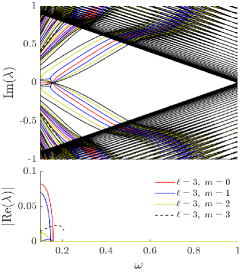
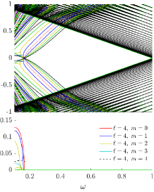
Figure 2: Spectrum for $\ell=3$ (left) and $\ell=4$ (right). Dashed black lines refer to quadruplets of eigenvalues with $\mathop{\rm{R\thinspace e}}\nolimits\lambda\neq 0$ bifurcating from the thresholds $\pm\mathrm{i}(1-\omega)$ (possibly a numerical artifact).

For $\ell=3$ (Fig. 2, left), for $m=0$, $\mathop{\rm{R\thinspace e}}\nolimits\lambda>0$ eigenvalue is born from the pitchfork bifurcation at $\omega_{p}\approx 0.159$. For $|m|=1$, quadruplets of eigenvalues appear when $\omega$ drops below $\omega\approx 0.155$ and then below $\omega\approx 0.147$ (the first one disappears at $\omega\approx 0.105$); for $|m|=2$, quadruplets appear at $\omega\approx 0.139$ and at $\omega\approx 0.106$ (all via HH bifurcations). For $|m|=3$, there is a quadruplet of $\mathop{\rm{R\thinspace e}}\nolimits\lambda\neq 0$ eigenvalues bifurcating from the thresholds $\pm\mathrm{i}(1-\omega)$ at $\omega\approx 0.2$, which is possibly a numerical artifact since the corresponding eigenfunctions do not seem to have a continuous limit.

For $\ell=4$ (Fig. 2, right), for $m=0$, unstable eigenvalue appears below pitchfork bifurcation at $\omega_{p}\approx 0.166$. For $|m|=1$, a quadruplet is born at $\omega\approx 0.159$; for $|m|=2$, another one appears at $\omega\approx 0.157$ (all via HH bifurcations). For $|m|=3$, a quadruplet of $\mathop{\rm{R\thinspace e}}\nolimits\lambda\neq 0$ eigenvalues bifurcating from the thresholds $\pm\mathrm{i}(1-\omega)$ when $\omega\approx 0.158$ again seems to be a numerical artifact. More quadruplets are born via HH bifurcations at $\omega\approx 0.148$ and $\omega\approx 0.13$ (the second disappears at $\omega\approx 0.116$). For $|m|=4$, a quadruplet of $\mathop{\rm{R\thinspace e}}\nolimits\lambda\neq 0$ eigenvalues bifurcates from the thresholds when $\omega\approx 0.17$.

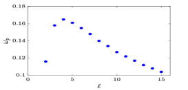
Figure 3: Value $\omega_{p}$ of pitchfork bifurcation

While the numerics show that larger $|m|$ lead to smaller intervals of instability (in agreement with (2+1)D case in [35]), the increase of $\ell$ seems to lead to the growth of the instability interval $(0,\omega_{p}(\ell))$. On Fig. 3, one can see that this tendency does not persist: the maximum value of $\omega_{p}\approx 0.166$ occurs for $\ell=4$; for larger $\ell$, the instability region $(0,\omega_{p}(\ell))$ is shrinking. Let us mention that there is an onset of instability for $\ell=1$ below the critical value $\omega_{p}\approx 0.07$, which is not presented on Figs. 1 and 3 since the numerics are not reliable for small $\omega$. Thus, the numerics suggest that the spectral stability region for both one-frequency and bi-frequency modes is $\omega\in(0.254M_{s},0.936M_{s})$.

I Conclusion

We showed the linear stability of some of one- and bi-frequency modes in the (cubic) Soler model via the radial reduction. The approach allows us to perform numerical computation of the spectrum of the linearization operator. We presented the numerical results based on the finite difference method, obtaining the stability region $\omega\in(0.254M_{s},0.936M_{s})$ for both one- and bi-frequency modes in the cubic Soler model in (3+1)D. The perturbation theory implies that there is a nearby stability region for localized modes of the DKG system. We suggest that stable bi-frequency modes can model neutral spinor particles from the Dark Matter sector which interact with the visible matter via the “Higgs portal”.

References

- Alexandrov [2008] A. S. Alexandrov, ed., Polarons in Advanced Materials, Materials Science, Vol. 103 (Springer, Dordrecht, 2008) pp. XVIII, 672.
- Everschor-Sitte et al. [2018] K. Everschor-Sitte, J. Masell, R. M. Reeve, and M. Kläui, Perspective: Magnetic skyrmions – Overview of recent progress in an active research field, J. Appl. Phys. 124, 240901 (2018).
- Franchini et al. [2021] C. Franchini, M. Reticcioli, M. Setvin, and U. Diebold, Polarons in materials, Nature Reviews Materials 6, 560 (2021).
- Mühlbauer et al. [2009] S. Mühlbauer, B. Binz, F. Jonietz, C. Pfleiderer, A. Rosch, A. Neubauer, R. Georgii, and P. Böni, Skyrmion lattice in a chiral magnet, Science 323, 915 (2009).
- Li et al. [2023] S. Li, X. Wang, and T. Rasing, Magnetic skyrmions: Basic properties and potential applications, Interdisciplinary Materials 2, 260 (2023).
- Berkolaiko and Comech [2012] G. Berkolaiko and A. Comech, On spectral stability of solitary waves of nonlinear Dirac equation in 1D, Math. Model. Nat. Phenom. 7, 13 (2012).
- Lakoba [2018] T. I. Lakoba, Numerical study of solitary wave stability in cubic nonlinear Dirac equations in 1D, Physics Letters A 382, 300 (2018).
- Merkl et al. [2010] M. Merkl, A. Jacob, F. E. Zimmer, P. Öhberg, and L. Santos, Chiral confinement in quasirelativistic Bose–Einstein condensates, Phys. Rev. Lett. 104, 073603 (2010).
- Smirnova et al. [2020] D. Smirnova, D. Leykam, Y. Chong, and Y. Kivshar, Nonlinear topological photonics, Applied Physics Reviews 7, 021306 (2020).
- Wang et al. [2016] B. Wang, E. Abdalla, F. Atrio-Barandela, and D. Pavon, Dark matter and dark energy interactions: theoretical challenges, cosmological implications and observational signatures, Reports on Progress in Physics 79, 096901 (2016).
- Soler [1970] M. Soler, Classical, stable, nonlinear spinor field with positive rest energy, Phys. Rev. D 1, 2766 (1970).
- Boussaïd and Comech [2018] N. Boussaïd and A. Comech, Spectral stability of bi-frequency solitary waves in Soler and Dirac–Klein–Gordon models, Commun. Pure Appl. Anal. 17, 1331 (2018).
- Galindo [1977] A. Galindo, A remarkable invariance of classical Dirac Lagrangians, Lett. Nuovo Cimento (2) 20, 210 (1977).
- Grillakis et al. [1990] M. Grillakis, J. Shatah, and W. Strauss, Stability theory of solitary waves in the presence of symmetry. II, J. Funct. Anal. 94, 308 (1990).
- Arcadi et al. [2020] G. Arcadi, A. Djouadi, and M. Raidal, Dark Matter through the Higgs portal, Physics Reports 842, 1 (2020).
- Cao et al. [2009] Q.-H. Cao, E. Ma, and G. Shaughnessy, Dark matter: the leptonic connection, Physics Letters B 673, 152 (2009).
- Boehmer et al. [2010] C. G. Boehmer, J. Burnett, D. F. Mota, and D. J. Shaw, Dark spinor models in gravitation and cosmology, Journal of High Energy Physics 2010, 1 (2010).
- Bai and Berger [2014] Y. Bai and J. Berger, Lepton portal dark matter, Journal of High Energy Physics 2014, 1 (2014).
- Bahamonde et al. [2018] S. Bahamonde, C. G. Böhmer, S. Carloni, E. J. Copeland, W. Fang, and N. Tamanini, Dynamical systems applied to cosmology: dark energy and modified gravity, Physics Reports 775, 1 (2018).
- Alves et al. [2015] A. Alves, F. de Campos, M. Dias, and J. M. Hoff da Silva, Searching for Elko dark matter spinors at the CERN LHC, International Journal of Modern Physics A 30, 1550006 (2015).
- Phillips et al. [2016] D. Phillips, W. Snow, K. Babu, S. Banerjee, D. Baxter, Z. Berezhiani, M. Bergevin, S. Bhattacharya, G. Brooijmans, L. Castellanos, M.-C. Chen, C. Coppola, R. Cowsik, J. Crabtree, P. Das, E. Dees, A. Dolgov, P. Ferguson, M. Frost, T. Gabriel, A. Gal, F. Gallmeier, K. Ganezer, E. Golubeva, G. Greene, B. Hartfiel, A. Hawari, L. Heilbronn, C. Johnson, Y. Kamyshkov, B. Kerbikov, M. Kitaguchi, B. Kopeliovich, V. Kopeliovich, V. Kuzmin, C.-Y. Liu, P. McGaughey, M. Mocko, R. Mohapatra, N. Mokhov, G. Muhrer, H. Mumm, L. Okun, R. Pattie, C. Quigg, E. Ramberg, A. Ray, A. Roy, A. Ruggles, U. Sarkar, A. Saunders, A. Serebrov, H. Shimizu, R. Shrock, A. Sikdar, S. Sjue, S. Striganov, L. Townsend, R. Tschirhart, A. Vainshtein, R. Van Kooten, Z. Wang, and A. Young, Neutron-antineutron oscillations: Theoretical status and experimental prospects, Physics Reports 612, 1 (2016).
- Berezhiani and Bento [2006] Z. Berezhiani and L. Bento, Neutron–mirror-neutron oscillations: How fast might they be?, Phys. Rev. Lett. 96, 081801 (2006).
- Kamyshkov et al. [2022] Y. Kamyshkov, J. Ternullo, L. Varriano, and Z. Berezhiani, Neutron-mirror neutron oscillations in absorbing matter, Symmetry 14, 10.3390/sym14020230 (2022).
- Broussard et al. [2022] L. Broussard, J. Barrow, L. DeBeer-Schmitt, T. Dennis, M. Fitzsimmons, M. Frost, C. Gilbert, F. Gonzalez, L. Heilbronn, E. Iverson, et al., Experimental search for neutron to mirror neutron oscillations as an explanation of the neutron lifetime anomaly, Phys. Rev. Lett. 128, 212503 (2022).
- Dvali et al. [2024] G. Dvali, M. Ettengruber, and A. Stuhlfauth, Kaluza–Klein spectroscopy from neutron oscillations into hidden dimensions, Phys. Rev. D 109, 055046 (2024).
- Berezhiani [2019] Z. Berezhiani, Neutron lifetime puzzle and neutron–mirror neutron oscillation, The European Phys. J. C 79, 1 (2019).
- Goldman et al. [2022] I. Goldman, R. N. Mohapatra, S. Nussinov, and Y. Zhang, Neutron–mirror-neutron oscillation and neutron star cooling, Phys. Rev. Lett. 129, 061103 (2022).
- Boyarsky et al. [2019] A. Boyarsky, M. Drewes, T. Lasserre, S. Mertens, and O. Ruchayskiy, Sterile neutrino Dark Matter, Progress in Particle and Nuclear Physics 104, 1 (2019).
- Dasgupta and Kopp [2021] B. Dasgupta and J. Kopp, Sterile neutrinos, Physics Reports 928, 1 (2021).
- Krasnov and Percacci [2018] K. Krasnov and R. Percacci, Gravity and unification: a review, Classical and Quantum Gravity 35, 143001 (2018).
- Ivanenko [1938] D. D. Ivanenko, Notes to the theory of interaction via particles, Zh. Eksper. Teoret. Fiz 8, 260 (1938).
- Esteban and Séré [1995] M. J. Esteban and É. Séré, Stationary states of the nonlinear Dirac equation: a variational approach, Comm. Math. Phys. 171, 323 (1995).
- Boussaïd and Comech [2017] N. Boussaïd and A. Comech, Nonrelativistic asymptotics of solitary waves in the Dirac equation with Soler-type nonlinearity, SIAM J. Math. Anal. 49, 2527 (2017).
- Boussaïd and Comech [2019] N. Boussaïd and A. Comech, Nonlinear Dirac equation. Spectral stability of solitary waves, Mathematical Surveys and Monographs, Vol. 244 (American Mathematical Society, Providence, RI, 2019).
- Cuevas-Maraver et al. [2016] J. Cuevas-Maraver, P. G. Kevrekidis, A. Saxena, A. Comech, and R. Lan, Stability of solitary waves and vortices in a 2D nonlinear Dirac model, Phys. Rev. Lett. 116, 214101 (2016).
- Berkolaiko et al. [2015] G. Berkolaiko, A. Comech, and A. Sukhtayev, Vakhitov–Kolokolov and energy vanishing conditions for linear instability of solitary waves in models of classical self-interacting spinor fields, Nonlinearity 28, 577 (2015).