Computing Barycentres of Measures for Generic Transport Costs

Abstract

Wasserstein barycentres represent average distributions between multiple probability measures for the Wasserstein distance. The numerical computation of Wasserstein barycentres is notoriously challenging. A common approach is to use Sinkhorn iterations, where an entropic regularisation term is introduced to make the problem more manageable. Another approach involves using fixed-point methods, akin to those employed for computing Fréchet means on manifolds. The convergence of such methods for 2-Wasserstein barycentres, specifically with a quadratic cost function and absolutely continuous measures, was studied by Alvarez-Esteban et al. in [6]. In this paper, we delve into the main ideas behind this fixed-point method and explore how it can be generalised to accommodate more diverse transport costs and generic probability measures, thereby extending its applicability to a broader range of problems. We show convergence results for this approach and illustrate its numerical behaviour on several barycentre problems.

1 Introduction

1.1 Related Works and Motivation

Wasserstein barycentres represent a powerful concept in Optimal Transport theory, enabling the computation of average distributions between multiple probability measures. These barycentres preserve the geometric structure of the underlying distributions, making them particularly suited for machine learning tasks. They have proven useful in numerous applications, including image processing [34], computer graphics [36, 14], statistics [13], domain adaptation [31], generative modelling [27], fairness in machine learning [24] or model selection in Bayesian learning [8]. Wasserstein barycentres are also at the core of clustering methods such as K-means, to define centroids in spaces of probability measures [25, 30].

The classical notion of barycentre refers to the weighted average of a set of points $(x_{k})$ with positive weights $(\lambda_{k})$ summing to $1$, in a metric space $(E,d)$. Formally, a barycentre $\bar{x}$ is a point that minimises the weighted sum of (typically squared) distances:

$$\bar{x}\in\underset{x\in E}{\operatorname{argmin}}\sum_{k=1}^{K}\lambda_{k}d^{2}(x,x_{k}).$$

This concept can be extended to the space of probability measures, where $d$ can be replaced for instance by a transportation cost $\mathcal{T}_{c}$. We remind that for two probability measures $\mu$ and $\nu$ on metric spaces $(\mathcal{X},d_{\mathcal{X}})$ and $(\mathcal{Y},d_{\mathcal{Y}})$, and a cost function $c:\mathcal{X}\times\mathcal{Y}\rightarrow\mathbb{R}_{+}$, the optimal transport cost between $\mu$ and $\nu$ for the ground cost $c$ is defined as

$$\mathcal{T}_{c}(\mu,\nu)=\underset{\pi\in\Pi(\mu,\nu)}{\inf}\int_{\mathcal{X}\times\mathcal{Y}}c\mathrm{d}\pi,$$

where $\Pi(\mu,\nu)$ is the set of probability measures on $\mathcal{X}\times\mathcal{Y}$ with marginals $\mu$ and $\nu$. Considering $K$ different cost functions $c_{k}$, the barycentre problem can be written in this setting as

$$\bar{\mu}\in\underset{\mu}{\operatorname{argmin}}\sum_{k=1}^{K}\lambda_{k}\mathcal{T}_{c_{k}}(\mu,\nu_{k}).$$ (1)

When $(\mathcal{X},d_{\mathcal{X}})=(\mathcal{Y},d_{\mathcal{Y}})$ is a Polish space and $c=d_{\mathcal{X}}^{p}$ with $p\geq 1$, $\mathrm{W}_{p}(\mu,\nu):=\left(\mathcal{T}_{d^{p}}(\mu,\nu)\right)^{\frac{1}{p}}$ defines a distance between probability measures (with finite moment of order $p$), called $p$-Wasserstein distance. In this case, the barycentre $\bar{\mu}$ defined above is called a Wasserstein barycentre. Generalisation to a barycentre of a probability measure on $\mathcal{P}(\mathcal{X})$ and the consistency of their discrete approximations is also studied by several authors [2].

The theoretical analysis of Wasserstein barycentres begins with the foundational work by Carlier and Ekeland [18], who studied the existence, uniqueness and dual formulations for barycentre problems with generic continuous cost functions. Subsequent work by [1] re-established the existence and dual formulations of such barycentres for the quadratic Wasserstein distance $\mathrm{W}_{2}$ on Euclidean spaces, and showed uniqueness under the hypothesis that one of the original measures is absolutely continuous. More recent studies have broadened these results:  [17] extended the theoretical analysis to Wasserstein medians ($\mathrm{W}_{1}$), studying their stability properties, and investigated dual and multi-marginal formulations. [16] further extended the framework to $\mathrm{W}_{p}$ distances for $p>1$, proving existence and uniqueness of barycentres for absolutely continuous measures on $\mathbb{R}^{d}$. A follow-up study by [15] analysed the general case for strictly convex and $\mathcal{C}^{2}$ cost functions with non-degenerate Hessian.

From a computational perspective, calculating Wasserstein barycentres is known to be a highly challenging problem, classified as NP-hard. According to [5], although polynomial-time algorithms exist for computing Wasserstein barycentres with a fixed number of points, their computational complexity scales exponentially with respect to the dimension of the space, or with respect to the number of marginals. This makes direct computation infeasible for high-dimensional problems or large sets of distributions, which are common in practical applications.

To tackle these computational challenges, several approximate methods have been developed for Wasserstein barycentres. The first paper to propose an algorithmic solution for computing these barycentres was by [34], which computed Sliced Wasserstein barycentres through a gradient descent approach. This method leveraged the sliced Wasserstein distance to achieve an efficient approximation, significantly simplifying computations.

A natural approach to develop easily computable approximations of such barycentres is to replace transport costs $\mathcal{T}_{c}$ by regularised versions

$$\mathcal{T}_{c,\varepsilon}(\mu,\nu)=\underset{\pi\in\Pi(\mu,\nu)}{\inf}\int_{\mathcal{X}\times\mathcal{Y}}c\mathrm{d}\pi+\varepsilon\operatorname{KL}(\pi|\mu\otimes\nu),$$

as proposed in [19]. When the support of the distributions and barycentre is fixed (a grid for instance), the problem can be rewritten as a KL projection problem and the so-called entropic barycentre can be computed efficiently with a modified version of Sinkhorn’s algorithm [11, 32].

In order to deal with distributions without imposed support a second approach also described in [19] relies on a fixed-point algorithm inspired by the computation of Fréchet means on manifolds. Each step of this fixed point approach consists in replacing the current barycentre $\mu$ by its image measure by the map $\sum_{k=1}^{K}\lambda_{k}T_{k}$, where the $T_{k}$ are optimal maps between $\mu$ and $\nu_{k}$ (assuming these maps exist). The authors of [6] were the first to establish a rigorous proof of convergence for this fixed-point approach in the case of absolutely continuous measures $\nu_{k}$: more precisely, they proved convergence of a subsequence to a fixed point and showed that if the fixed point is unique, it is indeed a barycentre. Their study focuses specifically on the case of $\mathrm{W}_{2}$ barycentres, with applications demonstrated mainly on Gaussian measures. Although their proof is only provided for absolutely continuous measures, this fixed point approach is frequently used for discrete measures and probably the baseline free-support method provided in numerical optimal transport libraries [22]. Building on the same ideas as [6], the author of [28] extends the investigation of the fixed point algorithm for discrete measures on $\mathbb{R}^{d}$, limited to just one single iteration, and deriving a worst-case error bound in the $\mathrm{W}_{2}$ and $\mathrm{W}_{1}$ settings. The iterative solver of  [6] has also been extended in high dimensional settings by [27], which use a neural solver for computing the optimal maps $T_{k}$.

In closely related directions, several other approaches have been proposed to compute Wasserstein barycentres over Riemannian manifolds [26], or Gromov-Wasserstein barycentres [9, 10] and the approach we develop in this paper share similarities with [9].

1.2 Contributions and Outline

In this paper, we develop a fixed-point approach to compute barycentres between probability measures for generic transport costs, i.e. solutions of the optimisation problem (1). Our only hypotheses are that we work on compact spaces, and that the ground costs $c_{k}$ are continuous and such that $\operatorname{argmin}_{x}\sum_{k=1}^{K}\lambda_{k}c_{k}(x,x_{k})$ is uniquely defined. In particular, we do not assume existence of optimal transport maps between $\mu$ and the $\nu_{k}$, and we do not assume anything on the probability measures $\mu$ and $\nu_{k}$. We propose an iterative fixed-point algorithm generalising [6] in this generic case. We show that the sequences generated by this algorithm have converging sub-sequences, that limits must be fixed-points of a certain mapping $G$, and that a barycentre for (1) is also a fixed point of $G$. We show that these results still hold for entropic regularised transport costs.

Numerically, we show that our approach specifically allows to extend the recent definition of generalised Wasserstein barycentres presented in [21], notably by considering non-linear functions between the ambient space and the subspaces of measures $\nu_{k}$. It also enables efficient computation of barycentres for the mixture Wasserstein metric [20], which until now were calculated using their multi-marginal equivalent formulation.

The paper is organised as follows. In Section˜2, we introduce a novel notion of Optimal Transport barycentres in a certain space between measures $\nu_{k}$ on potentially different spaces for generic costs $c_{k}$. In Section˜3, we propose a fixed-point algorithm which generalises [6] and converges to solutions (in a certain sense). We re-write the problem in a discrete setting in Section˜4 and illustrate our method in Section˜5 on several numerical examples, providing a publicly available Python toolkit.

2 Lifting Ground Barycentres to Measures

We work with probability measures $\nu_{k}$ on compact metric spaces $(\mathcal{Y}_{k},d_{\mathcal{Y}_{k}})_{k\in\llbracket 1,K\rrbracket}$, of which we will seek a "barycentre" $\mu$ in a compact metric space $(\mathcal{X},d_{\mathcal{X}})$. To compare a measure $\nu_{k}\in\mathcal{P}(\mathcal{Y}_{k})$ and $\mu\in\mathcal{P}(\mathcal{X})$ we consider continuous cost functions $c_{k}:\mathcal{X}\times\mathcal{Y}_{k}\longrightarrow\mathbb{R}_{+}$. A barycentre will be a minimiser of the sum of the transport costs with respect to the measure $\nu_{k}$, leading to the following energy for a measure $\mu\in\mathcal{P}(\mathcal{X})$:

$$V(\mu):=\sum_{k=1}^{K}\mathcal{T}_{c_{k}}(\mu,\nu_{k}),$$ (2)

hence our minimisation problem reads

$$\underset{\mu\in\mathcal{P}(\mathcal{X})}{\operatorname{argmin}}\ V(\mu).$$ (3)

Note that to introduce barycentre weights $\lambda_{k}$, it suffices to replace $c_{k}$ with $\lambda_{k}c_{k}$, which allows us to include weights in the costs and alleviate notation. We summarise our standing assumptions on the spaces and costs in ˜1:

Assumption 1.

The metric spaces $(\mathcal{X},d_{\mathcal{X}})$ and $(\mathcal{Y}_{k},d_{\mathcal{Y}_{k}})$ are compact, and the costs $c_{k}:\mathcal{X}\times\mathcal{Y}_{k}\longrightarrow\mathbb{R}_{+}$ are continuous.

Existence of solutions for Problem (3) was established by [18] Proposition 2 under ˜1.

Remark 2.1.

Uniqueness was proven in [18] Proposition 4 if, essentially, for at least one $k$, the problem $\mathcal{T}_{c_{k}}(\mu,\nu_{k})$ has a Monge solution, for which they assume that each $\nu_{k}$ is absolutely continuous on $\mathcal{Y}_{k}=\overline{\Omega}$ with $\Omega$ an open and bounded subset of $\mathbb{R}^{d}$ with with $\nu_{k}(\partial\Omega)=0$. They also assume that the costs $c_{k}(\cdot,y)$ are Lipschitz with a uniform constant $L$ and that $c_{k}$ verifies the Twist condition: $c_{k}(\cdot,y)$ is differentiable, with $\partial_{x}c_{k}(x,\cdot)$ injective.

The definition of a barycentre between measures $\nu_{k}$ can be seen as a lifting of a notion of barycentre within $\mathcal{X}$ of points $(y_{1},\cdots,y_{K})\in\mathcal{Y}_{1}\times\cdots\times\mathcal{Y}_{K}$. To give mathematical meaning to this intuition and to our method, we will make the following assumption throughout the paper:

Assumption 2.

For all $(y_{1},\cdots,y_{K})\in\mathcal{Y}_{1}\times\cdots\times\mathcal{Y}_{K},$ the set $\underset{x\in\mathcal{X}}{\operatorname{argmin}}\ \sum_{k=1}^{K}c_{k}(x,y_{k})$ has a unique element.

The uniqueness of the optimisation problem in ˜2 allows us to introduce the ground barycentre function $B$:

$$B:\left\{\begin{array}[]{ccc}\mathcal{Y}_{1}\times\cdots\times\mathcal{Y}_{K}&\longrightarrow&\mathcal{X}\\ (y_{1},\cdots,y_{K})&\longmapsto&\underset{x\in\mathcal{X}}{\operatorname{argmin}}\ \sum_{k=1}^{K}c_{k}(x,y_{k}).\\ \end{array}\right.$$ (4)

For convenience, we introduce $\mathcal{Y}:=\Pi_{k}\mathcal{Y}_{k},$ equipped with the product distance, with the notation $Y:=(y_{1},\cdots,y_{K})$ for an element of $\mathcal{Y}$, as well as the total cost function:

$$C:=\left\{\begin{array}[]{ccc}\mathcal{X}\times\mathcal{Y}&\longrightarrow&\mathbb{R}_{+}\\ (x,y_{1},\cdots,y_{K})&\longmapsto&\sum_{k=1}^{K}c_{k}(x,y_{k})\\ \end{array}\right..$$ (5)

Equipped with these convenient notations, we can write the multi-marginal formulation of our barycentre problem:

$$\underset{\pi\in\Pi(\nu_{1},\cdots,\nu_{K})}{\operatorname{argmin}}\int_{\mathcal{Y}}C(B(Y),Y)\mathrm{d}\pi(Y).$$ (6)

The barycentre problem defined in Eq.˜3 is related to the multi-marginal formulation through the following equation, due to [18], Proposition 3.3:

$$\underset{\mu\in\mathcal{P}(\mathcal{X})}{\operatorname{argmin}}\ V(\mu)=B\#\underset{\pi\in\Pi(\nu_{1},\cdots,\nu_{K})}{\operatorname{argmin}}\int_{\mathcal{Y}}C(B(Y),Y)\mathrm{d}\pi(Y).$$ (7)

The following technical result uses the continuity of the $c_{k}$ and ˜2 to show that $B$ is continuous.

Lemma 2.2.

The function $B:\mathcal{Y}\longrightarrow\mathcal{X}$ defined in Eq.˜4 is continuous.

Proof.

The proof uses standard compactness arguments, showing that for $Y_{n}\xrightarrow[n\longrightarrow+\infty]{}Y\in\mathcal{Y}$, $(B(Y_{n}))$ can only have $B(Y)$ as a subsequential limit. ∎

Another important technical result is the regularity of transport costs, which we will use repeatedly. We gather well-known results in Lemma˜2.3.

Lemma 2.3.

Consider $E,F$ compact metric spaces and let $c:E\times F\longrightarrow\mathbb{R}_{+}$ a measurable cost function. The optimal transport cost $\mathcal{T}_{c}$ has the following regularity for the weak convergence of measures depending on $c$:

1. If $c$ is lower-semi-continuous, then $\mathcal{T}_{c}$ is lower-semi-continuous.

2. If $c$ is continuous, then $\mathcal{T}_{c}$ is continuous.

3. If $E=F$ and $c$ is l.s.c. with $c(x,y)=0\Longrightarrow x=y$, then $\mathcal{T}_{c}(\mu,\nu)=0\Longrightarrow\mu=\nu$.

Proof.

Regarding item 1), by [35] Theorem 1.42, Kantorovich duality holds for $c$ l.s.c. and thus $\mathcal{T}_{c}$ can be written as a supremum of l.s.c. functions, hence is l.s.c.. For item 2), the result is verbatim [35] Theorem 1.51. For item 3), if $\mathcal{T}_{c}(\mu,\nu)=0$ then there exists $\pi\in\Pi(\mu,\nu)$ such that $\int_{E^{2}}c(x,y)\mathrm{d}\pi(x,y)=0$ (existence follows from lower semi-continuity, as in [35] Theorem 1.5). Thus for $\pi$-almost-every $(x,y)$, $c(x,y)=0$, which by assumption gives $x=y$, hence (using the same technique as in [35] Proposition 5.1) for any test function $\phi\in\mathcal{C}^{0}(E,\mathbb{R})$:

$$\int_{E}\phi(x)\mathrm{d}\mu(x)=\int_{E^{2}}\phi(x)\mathrm{d}\pi(x,y)=\int_{E^{2}}\phi(y)\mathrm{d}\pi(x,y)=\int_{E}\phi(y)\mathrm{d}\nu(y),$$

which shows that $\mu=\nu$. ∎

3 A Fixed-Point Algorithm

3.1 Algorithm Definition

In this section, we define a sequence $(\mu_{t})\in\mathcal{P}(\mathcal{X}){N}$ that will approach a barycentre of fixed measures $\nu_{k}\in\mathcal{P}(\mathcal{Y}_{k})$. We propose a modified version of the iterated scheme from [6] to solve Eq.˜3. To define an iteration mapping, for $\mu\in\mathcal{P}(X)$, we consider the set of multi-marginal couplings

$$\Gamma(\mu):=\left\{\gamma\in\mathcal{P}(\mathcal{X}\times\mathcal{Y}_{1}\times\cdots\times\mathcal{Y}_{K})\ :\ \forall k\in\llbracket 1,K\rrbracket,\;\gamma_{0,k}\in\Pi_{c_{k}}^{*}(\mu,\nu_{k})\right\},$$ (8)

where, for all $k$, $\gamma_{0,k}$ denotes the $\mathcal{X}\times\mathcal{Y}_{k}$ marginal of $\gamma$ and $\Pi_{c_{k}}^{*}(\mu,\nu_{k})$ denotes the set of all optimal couplings for the transport problem between $\mu$ and $\nu_{k}$ associated to the cost function $c_{k}$. The existence of such multi-couplings is a consequence of the well-known "gluing lemma" (see [35] Lemma 5.5). The following multi-coupling provides an explicit element of $\Gamma(\mu)$ given $\pi_{k}\in\Pi_{c_{k}}^{*}(\mu,\nu_{k})$:

$$\gamma(\mathrm{d}x,\mathrm{d}y_{1},\cdots,\mathrm{d}y_{K}):=\mu(\mathrm{d}x)\pi_{1}^{x}(\mathrm{d}y_{1})\cdots\pi_{K}^{x}(\mathrm{d}y_{K}),$$ (9)

where we wrote the disintegration of $\pi_{k}$ with respect to its first marginal $\mu$ as $\pi_{k}(\mathrm{d}x,\mathrm{d}y_{k})=\mu(\mathrm{d}x)\pi_{k}^{x}(\mathrm{d}y_{k})$. By abuse of notation, we will denote $B\#\gamma:=B\#\gamma_{1,\cdots,K}$, where $\gamma_{1,\cdots,K}\in\mathcal{P}(\mathcal{Y}_{1}\times\cdots\times\mathcal{Y}_{k})$ is the marginal of $\gamma$ with respect to $(y_{1},\cdots,y_{K})$. In terms of random variables, if $(X,Y_{1},\cdots,Y_{K})\sim\gamma$, then $B\#\gamma=\mathrm{Law}[B(Y_{1},\cdots,Y_{K})]$. Denoting $B\#\Gamma(\mu):=\{B\#\gamma,\;\gamma\in\Gamma(\mu)\}$, we define the multi-valued mapping $G$ which maps $\mu\in\mathcal{P}(\mathcal{X})$ to the set of next iterates $G(\mu)\subset\mathcal{P}(\mathcal{X})$:

$$G:=\left\{\begin{array}[]{ccc}\mathcal{P}(\mathcal{X})&\rightrightarrows&\mathcal{P}(\mathcal{X})\\ \mu&\mapsto&B\#\Gamma(\mu)\\ \end{array}\right..$$ (10)

Note that this construction is similar to that of [6], Remark 3.4. Moreover, the candidate barycentre $\overline{\mu}=B\#\gamma_{1,\cdots,K}$ is closely related to the multi-marginal formulation of the barycentre problem (see Eq.˜7). Indeed, set $\pi:=\gamma_{1,\cdots,K}\in\Pi(\mu_{1},\cdots,\mu_{K})$, notice that $\pi$ is a candidate for the multi-marginal problem of a particular structure induced by the reference measure $\mu$. In the case where the plans $\gamma_{0,k}$ are induced by maps $T_{k}$, then this structure is the coupling $(T_{1},\cdots,T_{K})\#\mu$. In terms of random variables, if $X\sim\mu$, then the chosen coupling is $(T_{1}(X),\cdots,T_{K}(X))$.

Taking inspiration from the $\mathrm{W}_{2}^{2}$ case, we can see informally the iterate $\overline{\mu}\in G(\mu)$ as a local linearisation of $\mathcal{P}(\mathcal{X})$. To illustrate this intuition, we consider the case $\mathcal{X}=\mathcal{Y}_{1}=\cdots=\mathcal{Y}_{K}$ and assume that for each $k$, the set of optimal plans $\Pi_{c_{k}}^{*}(\mu,\nu_{k})$ is reduced to $(I,T_{k})$, or in other words, that the Monge problem has a unique solution. Informally, one may see the set of maps $T:\mathcal{X}\longrightarrow\mathcal{X}$ sending $\mu$ to a measure $T\#\mu\in\mathcal{P}(\mathcal{X})$ as the tangent space to $\mathcal{P}(\mathcal{X})$ at $\mu$. As a result, the problem of finding a barycentre $\overline{\mu}$ can be seen from the viewpoint of the reference measure $\mu$ in the tangent space $T_{\mu}\mathcal{P}(\mathcal{X})$ as the problem of finding $S\in T_{\mu}\mathcal{P}(\mathcal{X})$ such that $S\#\mu$ would minimise the cost $V$. Our approach takes a barycentre of the optimal maps $T_{k}$ by choosing the candidate $S:=B\circ(T_{1},\cdots,T_{K})$. In the case of the squared-Euclidean cost on the common space $\mathbb{R}^{d}$, this amounts to $S:=\sum_{k}\lambda_{k}T_{k}$, which is exactly the Linearised Optimal Transport barycentre approximation for the reference measure $\mu$, as introduced in [29], Section 4.3. We illustrate this viewpoint schematically in Fig.˜1.

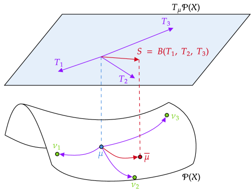
Figure 1: Illustration of the informal linearisation interpretation for the barycentre candidate $\overline{\mu}=B\circ(T_{1},\cdots,T_{K})\#\mu$.

Starting from a measure $\mu_{0}\in\mathcal{P}(\mathcal{X})$, our algorithm consists of choosing iterates through the multi-function $G$:

$$\forall t\in\mathbb{N},\;\mu_{t+1}\in G(\mu_{t}).$$

We dedicate the next section to a theoretical study of the convergence of this fixed-point iteration.

3.2 Convergence of Fixed-Point Iterations

We can formulate a regularity result of the multi-valued map $G$: namely, we will show that $G$ is upper hemi-continuous. For the sake of simplicity, we will take the following definition:

Definition 3.1.

A multi-valued function $\varphi:E\rightrightarrows F$ from a compact metric space $E$ to parts of a compact metric space $F$ is said to be upper hemi-continuous (u.h.c.) if for any sequence $(x_{n},y_{n})\in(E\times F){N}$ such that $y_{n}\in\varphi(x_{n})$ and $x_{n}\xrightarrow[n\longrightarrow+\infty]{}x\in E$, there exists an extraction such that $y_{\alpha(n)}\xrightarrow[n\longrightarrow+\infty]{}y\in F$ with $y\in\varphi(x)$.

For more technical reasons, we also need to introduce the notion of lower hemi-continuity

Definition 3.2.

A multi-valued function $\varphi:E\rightrightarrows F$ from a compact metric space space $E$ to parts of a compact metric space space $F$ is said to be lower hemi-continuous (l.h.c.) if for any sequence $(x_{n})\in E{N}$ such that $x_{n}\xrightarrow[n\longrightarrow+\infty]{}x\in E$, then for any $y\in F$ such that $y\in\varphi(x)$, there exists an extraction $\alpha$ and a sequence $(y_{n})\in F{N}$ such that $y_{n}\in\varphi(x_{\alpha(n)})$ and $y_{n}\xrightarrow[n\longrightarrow+\infty]{}y$.

To illustrate the technical differences between these two notions, we consider two specific multi-valued functions in Fig.˜2.

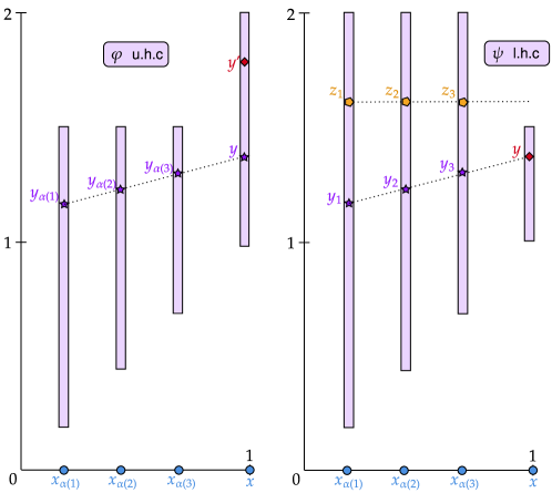
Figure 2: Left: the multi-function $\varphi:[0,1]\rightrightarrows[0,2]$ defined by $\forall x\in[0,1),\;\varphi(x)=[x,3/2]$ and $\varphi(1)=[1,2]$ is u.h.c.. Indeed, taking any sequence $(x_{n},y_{n})$ such that $y_{n}\in\varphi(x_{n})$ and $x_{n}\xrightarrow[n\longrightarrow+\infty]{}x$, there exists an extraction $\alpha$ such that $y_{\alpha(n)}\xrightarrow[n\longrightarrow+\infty]{}y\in\varphi(x)$. However, $\varphi$ is not l.h.c. at 1 since the target $y^{\prime}:=7/4\in\varphi(1)$ can never be a limit of a sequence $(x_{n},y_{n})$ with $x_{n}\xrightarrow[n\longrightarrow+\infty]{}1$ and $y_{n}\in\varphi(x_{n})$.
                                                  Right: $\psi:[0,1]\rightrightarrows[0,2]$ defined by $\forall x\in[0,1),\;\psi(x)=[x,2]$ and $\psi(1)=[1,3/2]$ is l.h.c.. Take $x_{n}\xrightarrow[n\longrightarrow+\infty]{}x$ and a target $y\in\psi(x)$. Then there exists an extraction $\alpha$ and a sequence $(y_{n})$ such that $y_{n}\in\psi(x_{n})$ and $y_{n}\xrightarrow[n\longrightarrow+\infty]{}y$. However, $\psi$ is not u.h.c: take $x_{n}\xrightarrow[n\longrightarrow+\infty]{}1$ and the sequence $z_{n}:=5/3$. We have $\forall n\in\mathbb{N},\;z_{n}\in\psi(x_{n})$, however any subsequence of $(z_{n})$ converges to $5/3\notin\psi(1)$.

Finally, an hemi-continuous multi-map is one that is both u.h.c. and l.h.c.:

Definition 3.3.

A multi-valued function $\varphi:E\rightrightarrows F$ from a compact metric space space $E$ to parts of a compact metric space space $F$ is said to be hemi-continuous if it is both u.h.c. (Definition˜3.1) and l.h.c. (Definition˜3.2).

We begin with technical lemmas on the hemi-continuity properties of sets of couplings.

Lemma 3.4.

Consider $E,F$ compact metric spaces and $\nu\in\mathcal{P}(F)$. The multi-function

$$\Pi_{\nu}:=\left\{\begin{array}[]{ccc}\mathcal{P}(E)&\rightrightarrows&\mathcal{P}(E\times F)\\ \mu&\mapsto&\Pi(\mu,\nu)\\ \end{array}\right.$$ (11)

is hemi-continuous.

Proof.

u.h.c.. We apply Definition˜3.1: introduce $\mu_{n}\xrightarrow[n\longrightarrow+\infty]{w}\mu\in\mathcal{P}(E)$ and $\pi_{n}\in\Pi(\mu_{n},\nu)$. Since $\mathcal{P}(E\times F)$ is compact, we can introduce $\alpha$ an extraction such that $\pi_{\alpha(n)}\xrightarrow[n\longrightarrow+\infty]{w}\pi\in\mathcal{P}(E\times F)$. By continuity of marginalisation, we deduce $\pi\in\Pi(\mu,\nu)$, which shows that $\Pi_{\nu}$ is u.h.c. by definition.

l.h.c.. We consider $\mathrm{W}_{1}$, the 1-Wasserstein distance on $\mathcal{P}(E)$ (i.e. $\mathcal{T}_{d_{E}}$), and use the same notation for the 1-Wasserstein distance on $\mathcal{P}(E^{2})$, with the distance $d_{E^{2}}((x,y),(x^{\prime},y^{\prime})):=\max(d_{E}(x,x^{\prime}),d_{E}(y,y^{\prime}))$, both of which metrise the weak convergence by [37] Corollary 6.13. We apply Definition˜3.2: take $\mu_{n}\xrightarrow[n\longrightarrow+\infty]{w}\mu\in\mathcal{P}(E)$, and let $\pi\in\Pi(\mu,\nu)$. Consider $(X,Y)$ two coupled random variables of law $\pi$, and for $n\in\mathbb{N}$, take $X_{n}$ a random variable such that $(X,X_{n})$ is an optimal coupling for $\mathrm{W}_{1}(\mu,\mu_{n})$, and let $\pi_{n}:=\mathrm{Law}(X_{n},Y)$. We have

$$\mathrm{W}_{1}(\pi,\pi_{n})\leq\mathbb{E}\left[d_{E^{2}}\left((X,Y),(X_{n},Y)\right)\right]=\mathbb{E}\left[\max(d_{E}(X,X_{n}),d_{E}(Y,Y))\right]=\mathrm{W}_{1}(\mu,\mu_{n}),$$

then by metrisation, we get $\mathrm{W}_{1}(\mu,\mu_{n})\xrightarrow[n\longrightarrow+\infty]{}0$, then $\pi_{n}\xrightarrow[n\longrightarrow+\infty]{w}\pi$, concluding the proof that $\Pi_{\nu}$ is l.h.c.. ∎

We can apply Berge’s maximisation theorem to show that the set of optimal transport plans is upper hemi-continuous for a continuous cost function:

Lemma 3.5.

Consider $E,F$ compact metric spaces, a continuous cost $c:E\times F\longrightarrow\mathbb{R}_{+}$ and $\nu\in\mathcal{P}(F)$. The multi-function

$$[\Pi_{c}^{*}]_{\nu}:=\left\{\begin{array}[]{ccc}\mathcal{P}(E)&\rightrightarrows&\mathcal{P}(E\times F)\\ \mu&\mapsto&\Pi_{c}^{*}(\mu,\nu)\\ \end{array}\right.$$ (12)

is upper hemi-continuous.

Proof.

By compactness, the map $\pi\longmapsto\int_{E\times F}c\mathrm{d}\pi$ is continuous, and by Lemma˜3.4, the multi-map $\mu\rightrightarrows\Pi(\mu,\nu)$ is hemi-continuous (with compact values), hence by Berge’s maximisation theorem from [3] Theorem 17.31, the map

$$[\Pi_{c}^{*}]_{\nu}:\mu\longmapsto\Pi_{c}^{*}(\mu,\nu)=\underset{\pi\in\Pi(\mu,\nu)}{\operatorname{argmin}}\int_{E\times F}c\mathrm{d}\pi$$

is upper hemi-continuous. ∎

Remark 3.6.

The multifunction $[\Pi_{c}^{*}]_{\nu}$ is not lower hemi-continuous. Indeed, take the following points of $\mathbb{R}^{2}$:

$$\forall n\in\mathbb{N},\;x_{n}:=(-1,2^{-n}),\;y_{n}:=(1,-2^{-n}),\;x_{\infty}:=(-1,0),\;y_{\infty}:=(1,0),\;w:=(0,1),\;z:=(0,-1),$$

and the following discrete measures (see Fig.˜3):

$$\forall n\in\mathbb{N},\;\mu_{n}:=\cfrac{1}{2}(\delta_{x_{n}}+\delta_{y_{n}}),\;\mu_{\infty}:=\cfrac{1}{2}(\delta_{x_{\infty}}+\delta_{y_{\infty}}),\;\nu:=\cfrac{1}{2}(\delta_{w}+\delta_{z}).$$

We have $\mu_{n}\xrightarrow[n\longrightarrow+\infty]{w}\mu_{\infty}$, and a unique OT plan for the cost $c(\cdot,\cdot):=\|\cdot-\cdot\|_{2}^{2}$ between $\mu_{n}$ and $\nu$, which sends $x_{n}$ to $w$ and $y_{n}$ to $z$:

$$\forall n\in\mathbb{N},\;\Pi_{c}^{*}(\mu_{n},\nu)=\{\pi_{n}\},\;\pi_{n}:=\cfrac{1}{2}\left(\delta_{x_{n},w}+\delta_{y_{n},z}\right),$$

with $\pi_{n}\xrightarrow[n\longrightarrow+\infty]{w}\pi_{\infty}:=\cfrac{1}{2}\left(\delta_{x_{\infty},w}+\delta_{y_{\infty},z}\right)$. However, the set of optimal plans between the limit $\mu_{\infty}$ and $\nu$ has more than one element, since $\|x_{\infty}-w\|_{2}^{2}=\|x_{\infty}-z\|_{2}^{2}$ and $\|y_{\infty}-w\|_{2}^{2}=\|y_{\infty}-z\|_{2}^{2}$:

$$\Pi_{c}^{*}(\mu,\nu)=\left\{(1-t)\pi_{\infty}+t\pi^{\prime},\;t\in[0,1]\right\},\;\pi^{\prime}:=\cfrac{1}{2}\left(\delta_{x_{\infty},z}+\delta_{y,w}\right).$$

We conclude that there does not exist an extraction $\alpha$ and a sequence $(\pi^{\prime}_{n})$ such that $\forall n\in\mathbb{N},\;\pi^{\prime}_{n}\in\Pi_{c}^{*}(\mu_{\alpha(n)},\nu)$ and $\pi^{\prime}_{n}\xrightarrow[n\longrightarrow+\infty]{w}\pi^{\prime}$.

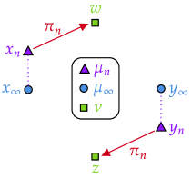
Figure 3: Counter-example from Remark˜3.6 showing that $\Pi_{c}^{*}(\cdot,\nu)$ is not lower hemi-continuous in general.

A direct corollary of Lemma˜3.5 is the upper hemi-continuity of $\Gamma$ and $G$. For notational convenience, we introduce $\mathcal{Z}:=\mathcal{X}\times\mathcal{Y}_{1}\times\cdots\times\mathcal{Y}_{K}$.

Proposition 3.7.

The multi-map

$$\Gamma:=\left\{\begin{array}[]{ccc}\mathcal{P}(\mathcal{X})&\rightrightarrows&\mathcal{P}(\mathcal{Z})\\ \mu&\mapsto&\Gamma(\mu)\\ \end{array}\right.$$

where $\Gamma(\mu)$ is defined in Eq.˜8 and $G$ defined in Eq.˜10 are upper hemi-continuous (and compact-valued).

Proof.

Let $\mu\in\mathcal{P}(\mathcal{X})$. To show that $G(\mu)$ and $\Gamma(\mu)$ are compact, it suffices to show that $\Gamma(\mu)$ is closed, since $\mathcal{P}(\mathcal{Z})$ is compact, and $G(\mu)=B\#\Gamma(\mu)$ with $B$ continuous by Lemma˜2.2. Take $(\gamma_{n})\in\Gamma(\mu){N}$ such that $\gamma_{n}\xrightarrow[n\longrightarrow+\infty]{}\gamma\in\mathcal{P}(\mathcal{Z})$. We show that $\gamma\in\Gamma(\mu)$. For $k\in\llbracket 1,K\rrbracket$ and $n\in\mathbb{N}$, we have $\gamma_{n}\in\Gamma(\mu)$, hence $[\gamma_{n}]_{0,k}\in\Pi_{c_{k}}^{*}(\mu,\nu_{k})$. By continuity of marginalisation, we deduce that $\gamma\in\Pi(\mu,\nu_{1},\cdots,\nu_{K})$. By continuity of $\pi\longmapsto\int_{\mathcal{X}\times\mathcal{Y}_{k}}c_{k}\mathrm{d}\pi$ (which holds by compactness), we deduce that $\gamma_{0,k}\in\Pi_{c_{k}}^{*}(\mu,\nu_{k})$, hence $\gamma\in\Gamma(\mu)$.

For the u.h.c. of $\Gamma$, take a sequence $(\mu_{n})\in\mathcal{P}(\mathcal{X}){N}$ such that $\mu_{n}\xrightarrow[n\longrightarrow+\infty]{w}\mu\in\mathcal{P}(\mathcal{X})$, and take a sequence $(\gamma_{n})\in\mathcal{P}(\mathcal{Z}){N}$, with $\gamma_{n}\in\Gamma(\mu_{n})$. Since $\gamma_{n}\in\mathcal{P}(\mathcal{Z})$ which is compact, take $\alpha$ an extraction such that $\gamma_{\alpha(n)}\xrightarrow[n\longrightarrow+\infty]{w}\gamma\in\mathcal{P}(\mathcal{Z})$. We will show that $\gamma\in\Gamma(\mu)$.

Start with $k:=1$. For $n\in\mathbb{N}$, we have $\gamma_{\alpha(n)}\in\Gamma(\mu_{\alpha(n)})$, hence $\pi_{\alpha(n)}^{(1)}:=[\gamma_{\alpha(n)}]_{0,1}\in\Pi_{c_{1}}^{*}(\mu_{\alpha(n)},\nu_{1})$. By Lemma˜3.5, the map $\mu\longmapsto\Pi_{c_{1}}^{*}(\mu,\nu_{1})$ is u.h.c., hence by definition, since $\mu_{\alpha(n)}\xrightarrow[n\longrightarrow+\infty]{w}\mu\in\mathcal{P}(\mathcal{X})$ and $\pi_{\alpha(n)}^{(1)}\in\Pi_{c_{1}}^{*}(\mu_{\alpha(n)},\nu_{1})$, there exists an extraction $\alpha_{1}$ such that $\pi_{\alpha\circ\alpha_{1}(n)}^{(1)}\xrightarrow[n\longrightarrow+\infty]{w}\pi^{(1)}\in\Pi_{c_{1}}^{*}(\mu,\nu_{1})$.

Continuing this method for $k\in\llbracket 2,K\rrbracket$ with successive sub-extractions $\alpha_{k}$, setting $\beta:=\alpha\circ\alpha_{1}\circ\cdots\circ\alpha_{K}$, we have for any $k\in\llbracket 1,K\rrbracket,\;[\gamma_{\beta(n)}]_{0,k}=\pi_{\beta(n)}^{(k)}\xrightarrow[n\longrightarrow+\infty]{w}\pi^{(k)}\in\Pi_{c_{k}}^{*}(\mu,\nu_{k})$. The continuity of marginalisation implies $\gamma_{0,k}=\pi^{(k)}$, and in turn shows that $\gamma\in\Gamma(\mu)$, concluding that $\Gamma$ is u.h.c.

For $G$, the fact that $G(\mu)=B\#\Gamma(\mu)$ and the continuity of $B$ prove that $G$ is u.h.c. using the u.h.c. of $\Gamma$ by [3] Theorem 17.23. ∎

In order to study the energy of iterates of $G$, we first require a technical result on the error of sub-optimal ground barycentres for $B$. We introduce a radius constant $R:=\underset{(x,Y)\in\mathcal{X}\times\mathcal{Y}}{\max}\ d_{\mathcal{X}}(x,B(Y))$, which is finite since $\mathcal{X}$ and $\mathcal{Y}$ are compact, and $B$ is continuous. We need to make a trivial assumption to ensure that $R>0$:

Assumption 3.

There exists $x\in\mathcal{X}$ and $Y\in\mathcal{Y}$ such that $x\neq B(Y)$.

Lemma˜3.8 is a generalisation of the following elementary Euclidean property in $\mathbb{R}^{d}$ for the cost $\|\cdot-\cdot\|_{2}^{2}$, for which $B(y_{1},\cdots,y_{K})=\sum_{k=1}^{K}\lambda_{k}y_{k}$ verifies the following identity:

$$\forall x\in\mathbb{R}^{d},\;\forall(y_{1},\cdots,y_{K})\in(\mathbb{R}^{d})^{K},\;\overline{x}:=\sum_{k=1}^{K}\lambda_{k}y_{k}:\;\sum_{k=1}^{K}\lambda_{k}\|x-y_{k}\|_{2}^{2}=\sum_{k=1}^{K}\lambda_{k}\|\overline{x}-y_{k}\|_{2}^{2}+\|x-\overline{x}\|_{2}^{2}.$$

Lemma 3.8.

There exists a function $\delta=\eta\circ d_{\mathcal{X}}$, with $\eta:[0,R]\longrightarrow\mathbb{R}_{+}$ lower-semi-continuous, non-decreasing and verifying $\eta(s)=0\Longleftrightarrow s=0$, such that

$$\forall(x,Y)\in\mathcal{X}\times\mathcal{Y},\;C(x,Y)\geq C(B(Y),Y)+\delta(x,B(Y)).$$ (13)

Proof.

— Step 1: Definition of $\eta$. First, for $(x,Y)\in\mathcal{X}\times\mathcal{Y}$, let $\Delta(x,Y):=C(x,Y)-C(B(Y),Y)$. By definition of $B$, $\Delta(x,Y)\geq 0$, and $\Delta(x,Y)=0\Longleftrightarrow x=B(Y)$. By assumption, $B$ and $C$ are continuous, which implies that $\Delta$ is also continuous.

We now introduce $S:=\max_{(x,Y)\in\mathcal{X}\times\mathcal{Y}}\Delta(x,Y)$. ˜3 ensures $S>0$. Define now the function $\eta$:

$$\eta:=\left\{\begin{array}[]{ccc}[0,R]&\longrightarrow&[0,S]\\ u&\longmapsto&\underset{(x,Y)\in\mathcal{X}\times\mathcal{Y}}{\min}\ \left\{\Delta(x,Y)\ :\ d_{\mathcal{X}}(x,B(Y))\geq u\right\}\\ \end{array}\right..$$ (14)

We show that for $u\in[0,R]$, the infimum is attained. First, let $f:=(x,Y)\longmapsto d_{\mathcal{X}}(x,B(Y))$, we remark that

$$\forall(x,Y)\in\mathcal{X}\times\mathcal{Y},\;d_{\mathcal{X}}(x,B(Y))\geq u\Longleftrightarrow(x,Y)\in f^{-1}([u,R]).$$

By continuity of $f$ and compactness of $\mathcal{X}\times\mathcal{Y}$, $\mathcal{K}_{u}:=f^{-1}([u,R])$ is a compact subset of $\mathcal{X}\times\mathcal{Y}$. $\mathcal{K}_{u}$ is not empty since there exists $(x_{R},Y_{R})\in\mathcal{X}\times\mathcal{Y}$ such that $d_{\mathcal{X}}(x_{R},B(Y_{R}))=R$ (by continuity, compactness and definition of $R$).

— Step 2: Proof of Eq.˜13. Let $(x,Y)\in\mathcal{X}\times\mathcal{Y}$, and $u:=d_{\mathcal{X}}(x,B(Y))$. By definition, $(x,Y)\in\mathcal{K}_{u}$, hence $\eta(u)\leq\Delta(x,Y)$, which is equivalent to Eq.˜13.

— Step 3: Lower semi-continuity of $\eta$. Let $u_{n}\xrightarrow[n\longrightarrow+\infty]{}u\in[0,R]$, and for $n\in\mathbb{N}$ introduce $(x_{n},Y_{n})\in\mathcal{K}_{u_{n}}$ such that $\eta(u_{n})=\Delta(x_{n},Y_{n})$. Since $(\eta(u_{n}))\in[0,S]{N}$, consider an extraction $\alpha$ such that $\eta(u_{\alpha(n)})\xrightarrow[n\longrightarrow+\infty]{}a_{\alpha}\in[0,S]$. By compactness of $\mathcal{X}\times\mathcal{Y}$, we can extract from $(x_{\alpha(n)},Y_{\alpha(n)})_{n}$ a subsequence such that $(x_{\alpha\circ\beta(n)},Y_{\alpha\circ\beta(n)})\xrightarrow[n\longrightarrow+\infty]{}(x_{\alpha,\beta},Y_{\alpha,\beta})\in\mathcal{X}\times\mathcal{Y}$. By construction of the sequence $(x_{n},Y_{n})_{n}$, we have

$$\forall n\in\mathbb{N},\;d_{\mathcal{X}}(x_{\alpha\circ\beta(n)},B(Y_{\alpha\circ\beta(n)}))\geq u_{\alpha\circ\beta(n)},$$ (15)

since $(x_{\alpha\circ\beta(n)},Y_{\alpha\circ\beta(n)})\in\mathcal{K}_{u_{\alpha\circ\beta(n)}}$. Taking the limit in Eq.˜15 yields $d_{\mathcal{X}}(x_{\alpha,\beta},B(Y_{\alpha,\beta}))\geq u,$ by continuity of $B$, Lemma˜2.2. This shows that $(x_{\alpha,\beta},Y_{\alpha,\beta})\in\mathcal{K}_{u}$, hence $\eta(u)\leq\Delta(x_{\alpha,\beta},Y_{\alpha,\beta})$. However, by continuity of $\Delta$, and since $\Delta(x_{\alpha(n)},Y_{\alpha(n)})\xrightarrow[n\longrightarrow+\infty]{}a_{\alpha}$, it follows that $\Delta(x_{\alpha,\beta},Y_{\alpha,\beta})=a_{\alpha}$. Since the subsequential limit $a_{\alpha}$ was chosen arbitrarily, we conclude that $\eta(u)\leq\underset{n\longrightarrow+\infty}{\liminf}\eta(u_{n})$, hence $\eta$ is lower semi-continuous.

— Step 4: $\eta$ is non-decreasing. Let $0\leq u\leq v\leq R$, we have $\mathcal{K}_{v}\subset\mathcal{K}_{u}$, hence

$$\eta(u)=\underset{(x,Y)\in\mathcal{K}_{u}}{\min}\ \Delta(x,Y)\leq\underset{(x,Y)\in\mathcal{K}_{v}}{\min}\ \Delta(x,Y)=\eta(v).$$

— Step 5: Separation property. Let $u\in[0,R]$ such that $\eta(u)=0$. This implies that there exists $(x,Y)\in\mathcal{X}\times\mathcal{Y}$ such that $\Delta(x,Y)=0$ and $d_{\mathcal{X}}(x,B(Y))\geq u$. Now by Step 1 this implies $x=B(Y)$, thus $d_{\mathcal{X}}(x,B(Y))=0$ and finally $u=0$. ∎

Given the inequality in Eq.˜13, we can now find an informative inequality between $V(\overline{\mu})$ and $V(\mu)$ for any $\overline{\mu}\in G(\mu)$. Applying ˜3.9 to the $\mathrm{W}_{2}$ case for absolutely continuous measures yields [6] Proposition 4.3, wherein the cost $\mathcal{T}_{\delta}$ is simply $\mathrm{W}_{2}^{2}$. This decrease was also studied by [28] (Proposition 4.4) in the discrete setting $\mathrm{W}_{p}^{p}$.

Proposition 3.9.

Let $\mu\in\mathcal{P}(\mathcal{X})$ and $\overline{\mu}\in G(\mu)$. Then $V(\mu)\geq V(\overline{\mu})+\mathcal{T}_{\delta}(\mu,\overline{\mu})$. If $\mu^{*}$ is a barycentre, then $G(\mu^{*})=\{\mu^{*}\}$.

Proof.

Let $\overline{\mu}=B\#\gamma\in G(\mu)$ with $\gamma\in\Gamma(\mu)$, by definition of $\mathcal{T}_{c_{k}}$ and by optimality of the bi-marginals $\gamma_{0,k}$ of $\gamma$:

$$\sum_{k=1}^{K}\mathcal{T}_{c_{k}}(\mu,\nu_{k}) =\int_{\mathcal{X}\times\mathcal{Y}}C(x,Y)\mathrm{d}\gamma(x,Y)$$ (16)

$$\geq\int_{\mathcal{X}\times\mathcal{Y}}(C(B(Y),Y)+\delta(x,B(Y)))\mathrm{d}\gamma(x,Y)$$ (17)

$$\geq\sum_{k=1}^{K}\mathcal{T}_{c_{k}}(B\#\gamma,\nu_{k})+\mathcal{T}_{\delta}(\mu,B\#\gamma)$$ (18)

$$=V(\overline{\mu})+\mathcal{T}_{\delta}(\mu,\overline{\mu}).$$ (19)

The inequality in Eq.˜17 comes from Lemma˜3.8, and the inequality in Eq.˜18 comes from the definition of $\Gamma(\mu)$ (Eq.˜8), which allows us to write for $k\in\llbracket 1,K\rrbracket$:

$$\int_{\mathcal{X}\times\mathcal{Y}}c_{k}(B(Y),y_{k})\mathrm{d}\gamma(x,Y) =\int_{\mathcal{X}\times\mathcal{Y}_{k}}c_{k}\mathrm{d}\pi_{k},$$

where we introduce the coupling $\pi_{k}:=(B,P_{k})\#[\gamma_{1,\cdots,K}]$, with $P_{k}(y_{1},\cdots,y_{K})=y_{k}$. The first marginal of $\pi$ is $B\#[\gamma_{1,\cdots,K}]$ (which we write $B\#\gamma$ for legibility), and the second marginal is $\nu_{k}$. Similarly,

$$\int_{\mathcal{X}\times\mathcal{Y}}\delta(x,B(Y))\mathrm{d}\gamma(x,Y)=\int_{\mathcal{X}\times\mathcal{X}}\delta\mathrm{d}[(I,B)\#\gamma]\geq\mathcal{T}_{\delta}(\mu,B\#\gamma).$$

If $\mu^{*}$ is a barycentre, then by definition for any $\overline{\mu}\in G(\mu)$, we have $V(\overline{\mu})\geq V(\mu^{*})$, thus Eqs.˜17 and 18 are equalities, and $\mathcal{T}_{\delta}(\mu^{*},\overline{\mu})=0$. By Lemmas˜3.8 and 2.3, the cost $\delta$ guarantees the separation property of the transport cost $\mathcal{T}_{\delta}$, hence $\mu^{*}=\overline{\mu}$. ∎

The inequality in ˜3.9 shows that the amount of decrease in the energy between two iterations is lower-bounded by a transport discrepancy $\mathcal{T}_{\delta}$ (we remind that in the squared-Euclidean case, $\mathcal{T}_{\delta}=\mathrm{W}_{2}^{2}$). We can now show convergence of iterates of $G$, in the sense that any weakly converging subsequence converges towards a fixed point of $G$.

Theorem 3.10.

For any $\mu_{0}\in\mathcal{P}(\mathcal{X})$, let $(\mu_{t})$ verifying $\mu_{t+1}\in G(\mu_{t})$. Then $(\mu_{t})$ has converging subsequences, and any weakly converging subsequence necessarily converges towards a $\mu\in\mathcal{P}(\mathcal{X})$ such that $\mu\in G(\mu)$.

Proof.

Fix a sequence $(\mu_{t})$ such that $\mu_{t+1}\in G(\mu_{t})$ and write $\mu_{t+1}=B\#[\gamma_{t}]_{1,\cdots,K}$ with $\gamma_{t}\in\Gamma(\mu_{t})$. Since $\mathcal{X}$ is compact, the space $\mathcal{P}(\mathcal{X})$ is also compact, and so the sequence $(\mu_{t})$ is tight. Consider an extraction $\alpha$ such that $\mu_{\alpha(t)}\xrightarrow[t\longrightarrow+\infty]{w}\mu\in\mathcal{P}(\mathcal{X})$. By u.h.c. of $\Gamma$ (˜3.7), there exists an extraction $\beta$ such that $\gamma_{\alpha\circ\beta(t)}\xrightarrow[t\longrightarrow+\infty]{w}\gamma\in\Gamma(\mu)$.

By ˜3.9, the sequence $(V(\mu_{t}))$ is non-increasing and non-negative, hence it is convergent, imposing $\underset{t\longrightarrow+\infty}{\lim}\left[V(\mu_{\alpha\circ\beta(t)})-V(\mu_{\alpha\circ\beta(t)+1})\right]=0$. Using the lower-bound in ˜3.9 we obtain:

$$\forall t\in\mathbb{N},\;0\leq\mathcal{T}_{\delta}(\mu_{\alpha\circ\beta(t)},\mu_{\alpha\circ\beta(t)+1})\leq V(\mu_{\alpha\circ\beta(t)})-V(\mu_{\alpha\circ\beta(t)+1}),$$

and take the limit inferior:

$$0\leq\underset{t\longrightarrow+\infty}{\liminf}\ \mathcal{T}_{\delta}(\mu_{\alpha\circ\beta(t)},\mu_{\alpha\circ\beta(t)+1})\leq 0.$$ (20)

We remind that $(\mu_{\alpha\circ\beta(t)+1})_{t}$ is a sequence in $\mathcal{P}(\mathcal{X})$ which is compact, and take $\rho\in\mathcal{P}(\mathcal{X})$ a subsequential limit of $(\mu_{\alpha\circ\beta(t)+1})_{t}$. By lower-semi-continuity of $\mathcal{T}_{\delta}$ (which holds by applying Lemma˜2.3 item 1) with Lemma˜3.8), Eq.˜20 provides $\mathcal{T}_{\delta}(\mu,\rho)=0$. By Lemma˜2.3 item 3), we obtain that $\rho=\mu$, thus any subsequential limit of $(\mu_{\alpha\circ\beta(t)+1})_{t}$ is $\mu$, which proves that it converges weakly to $\mu$.

Writing abusively $B\#\gamma$ for $B\#\gamma_{1,\cdots,K}$, we conclude:

$$\begin{array}[]{ccc}\mu_{\alpha\circ\beta(t)+1}&\xrightarrow[t\longrightarrow+\infty]{w}&\mu\\ \rotatebox{90.0}{$\,=$}&&\rotatebox{90.0}{$\,=$}\\ B\#\gamma_{\alpha\circ\beta(t)}&\xrightarrow[t\longrightarrow+\infty]{w}&B\#\gamma\\ \end{array}$$

hence we have found $\gamma\in\Gamma(\mu)$ such that $\mu=B\#\gamma$, proving $\mu\in G(\mu)$. ∎

3.3 Expression of the Iterates when the Plans are Maps

In some cases, the plans introduced in $\Gamma(\mu)$ (Eq.˜8) are induced by maps, which is to say that they are each supported on a set of the form $(x,T_{k}(x))$. This is the case in the specific setting chosen by [6], which is to say that all measures are absolutely continuous on $\mathbb{R}^{d}$ and the costs are all $c(x,y)=\|x-y\|_{2}^{2}$. By Brenier’s Theorem (as stated in [35], Theorem 1.22, for example), this implies that optimal transport couplings are supported on the graph of a map. This property holds under the weaker condition that the costs verify the Twist condition (see [37] Theorem 10.28 for example). In this case, each set optimal transport plans $\Pi_{c_{k}}^{*}(\mu,\nu_{k})$ is composed of one element $(I,T_{k})\#\mu$, and as a result, the expression of $G(\mu)$ becomes substantially simpler, namely $G(\mu)=\{B\circ(T_{1},\cdots,T_{K})\#\mu\}$. In the linearisation interpretation (Fig.˜1), this expression can be understood as taking the ground barycentre of the maps $T_{k}$ using the ground map $B$.

Drawing inspiration from this observation, we can define an alternative iteration consisting in choosing a map $T_{k}$ as the barycentric projection of the coupling $\gamma_{0,k}\in\Pi_{c_{k}}^{*}(\mu,\nu_{k})$ for $\gamma\in\Gamma(\mu)$: see Definition˜3.11 and Fig.˜4.

Definition 3.11.

The barycentric projection of a coupling $\pi\in\Pi(\mu,\nu)$ for $\mu\in\mathcal{P}(E)$ and $\nu\in\mathcal{P}(F)$ is the map $\overline{\pi}:E\longrightarrow F$, which is defined for $\mu$-almost-every $x\in E$ as:

$$\overline{\pi}(x)=\int_{F}y\pi_{x}(\mathrm{d}y),$$

where we wrote the disintegration $\pi(\mathrm{d}x,\mathrm{d}y)=\mu(\mathrm{d}x)\pi_{x}(\mathrm{d}y)$. In terms of random variables, one may write this expression as:

$$\overline{\pi}(x)=\underset{(X,Y)\sim\pi}{\mathbb{E}}[Y\ |\ X=x].$$

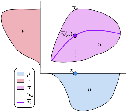
Figure 4: Illustration of a barycentric projection. The disintegration of the coupling $\pi$ with respect to its first marginal $\mu$ at $x$ is the measure $\pi_{x}$ concentrated on the dotted line. The barycentric projection of $\pi$ evaluated at $x$ is the mean of the measure $\pi_{x}$.

Note that for this expression to be well-defined, the target space $F$ must be a convex space, i.e. a space where one may define convex combinations of points (or, more precisely, expectations of probability measures). In the case $\mathcal{X}=\mathcal{Y}_{1}=\cdots=\mathcal{Y}_{K}$, a meaningful choice of convex combination is the ground barycentre $B$. We can apply this barycentric projection idea to define an alternate multi-mapping $H:\mathcal{P}(\mathcal{X})\rightrightarrows\mathcal{P}(\mathcal{X})$:

$$\forall\mu\in\mathcal{P}(\mathcal{X}),\;H(\mu):=\left\{B\circ(\overline{\gamma_{0,1}},\cdots,\overline{\gamma_{0,K}})\#\mu,\;\gamma\in\Gamma(\mu)\right\}.$$ (21)

In general, for $\pi\in\Pi(\mu,\nu),\;\overline{\pi}\#\mu\neq\nu$, hence one does not necessarily have $\forall\widetilde{\mu}\in H(\mu),\;V(\widetilde{\mu})\leq V(\mu)$. However, if each $\Pi_{c_{k}}^{*}(\mu,\nu_{k})$ are composed of plans supported by maps, then $H(\mu)=G(\mu)$. In the case of discrete measures and for the squared Euclidean cost, the iterations of $H$ correspond to the approach proposed in [19], Algorithm 2.

3.4 Extension to the Entropic Case

In this section, we explain how our results from Section˜3.2 extend to Entropic-Regularised Optimal transport, wherein we introduce for a regularisation $\varepsilon>0$:

$$\mathcal{T}_{c,\varepsilon}(\mu,\nu):=\underset{\pi\in\Pi(\mu,\nu)}{\min}\ \int_{E\times F}c\mathrm{d}\pi+\varepsilon\operatorname{KL}(\pi|\mu\otimes\nu),\quad V_{\varepsilon}:=\sum_{k=1}^{K}\mathcal{T}_{c_{k},\varepsilon}(\mu,\nu_{k}).$$ (22)

Strict convexity of the $\operatorname{KL}$ divergence yields existence and uniqueness of entropic optimal transport plans (denoted $\Pi_{c,\varepsilon}^{*}(\mu,\nu)$), and by [23] Theorem 1.4, the (single-valued) map $\mu\longmapsto\Pi_{c,\varepsilon}^{*}(\mu,\nu)$ is continuous for the weak convergence, provided that the cost $c$ is continuous. Akin to the OT case, we define the map $\Gamma_{\varepsilon}:\mathcal{P}(\mathcal{X})\longrightarrow\mathcal{P}(\mathcal{Z})$ by:

$$\Gamma_{\varepsilon}(\mu):=\mu(\mathrm{d}x)\pi_{1,\varepsilon}^{x}(\mathrm{d}y_{1})\cdots\pi_{K,\varepsilon}^{x}(\mathrm{d}y_{K}),\;\forall k\in\llbracket 1,K\rrbracket,\;\pi_{k,\varepsilon}:=\Pi_{c_{k},\varepsilon}^{*}(\mu,\nu_{k}),$$ (23)

and the iteration functional $G_{\varepsilon}(\mu):=B\#\Gamma_{\varepsilon}(\mu)$. Using Lemma˜3.8 and some technical manipulations of the $\operatorname{KL}$ divergence, we adapt ˜3.9 to this entropic case.

Proposition 3.12.

Let $\mu\in\mathcal{P}(\mathcal{X})$ and $\overline{\mu}:=G_{\varepsilon}(\mu)$. Then $V_{\varepsilon}(\mu)\geq V_{\varepsilon}(\overline{\mu})+\mathcal{T}_{\delta}(\mu,\overline{\mu})$. If $\mu^{*}$ is a barycentre, then $G_{\varepsilon}(\mu^{*})=\mu^{*}$.

Proof.

We begin as in ˜3.9, with $\gamma:=\Gamma_{\varepsilon}(\mu)$:

$$\sum_{k=1}^{K}\mathcal{T}_{c_{k},\varepsilon}(\mu,\nu_{k}) =\int_{\mathcal{X}\times\mathcal{Y}}C(x,Y)\mathrm{d}\gamma(x,Y)+\varepsilon\sum_{k=1}^{K}\operatorname{KL}(\gamma_{0,k}|\mu\otimes\nu_{k})$$ (24)

$$\geq\int_{\mathcal{X}\times\mathcal{Y}}(C(B(Y),Y)+\delta(x,B(Y)))\mathrm{d}\gamma(x,Y)+\varepsilon\sum_{k=1}^{K}\operatorname{KL}(\gamma_{0,k}|\mu\otimes\nu_{k}).$$ (25)

For convenience, write $\gamma_{\otimes}:=\mu\otimes\nu_{1}\otimes\cdots\otimes\nu_{K}$. Using the notation from Eq.˜23, notice that $\cfrac{\mathrm{d}\gamma}{\mathrm{d}\gamma_{\otimes}}=\prod_{k=1}^{K}\cfrac{\mathrm{d}\pi_{k,\varepsilon}}{\mathrm{d}(\mu\otimes\nu_{k})}$, which implies that $\sum_{k}\operatorname{KL}(\gamma_{0,k}|\mu\otimes\nu_{k})=\operatorname{KL}(\gamma|\gamma_{\otimes})$. Putting this with Eq.˜25 yields

$$V_{\varepsilon}(\mu)\geq\sum_{k=1}^{K}\int_{\mathcal{X}\times\mathcal{Y}_{k}}c_{k}\mathrm{d}(B,P_{k})\#\gamma+\varepsilon\operatorname{KL}(\gamma|\gamma_{\otimes})+\int_{\mathcal{X}^{2}}\delta\mathrm{d}(I,B)\#\gamma.$$ (26)

Now let $f:\mathcal{X}\times\mathcal{Y}_{1}\times\cdots\times\mathcal{Y}_{K}\longrightarrow\mathcal{X}\times\mathcal{Y}_{1}\times\cdots\times\mathcal{Y}_{K}$ the continuous function defined by $f(x,y_{1},\cdots,y_{K}):=(B(y_{1},\cdots,y_{K}),y_{1},\cdots,y_{K})$. We apply the data processing inequality (use the Donsker-Varadhan identity [33] Theorem 3.5): $\operatorname{KL}(\gamma|\gamma_{\otimes})\geq\operatorname{KL}(f\#\gamma|f\#\gamma_{\otimes}).$ Now we use the disintegration formula and the change-of-reference formula for $\operatorname{KL}$. Notice that the first marginals of $f\#\gamma$ and $f\#\gamma_{\otimes}$ are both equal to $\overline{\mu}$, and that $(f\#\gamma)_{1,\cdots,K}\in\Pi(\nu_{1},\cdots,\nu_{K})$ and $(f\#\gamma_{\otimes})_{1,\cdots,K}=\nu_{1}\otimes\cdots\otimes\nu_{K}$.

$$\operatorname{KL}(f\#\gamma|f\#\gamma_{\otimes}) =\operatorname{KL}((f\#\gamma)_{0}|(f\#\gamma_{\otimes})_{0})+\int_{\mathcal{X}}\operatorname{KL}((f\#\gamma)^{x}|\nu_{1}\otimes\cdots\otimes\nu_{K})\mathrm{d}\overline{\mu}(x)$$

$$=0+\int_{\mathcal{X}}\operatorname{KL}((f\#\gamma)^{x}|(f\#\gamma)^{x}_{1}\otimes\cdots\otimes(f\#\gamma)^{x}_{K})\mathrm{d}\overline{\mu}(x)$$

$$+\operatorname{KL}((f\#\gamma)^{x}_{1}\otimes\cdots\otimes(f\#\gamma)^{x}_{K}|\nu_{1}\otimes\cdots\otimes\nu_{K})\mathrm{d}\overline{\mu}(x)$$

$$\geq\sum_{k=1}^{K}\int_{\mathcal{X}}\operatorname{KL}((f\#\gamma)^{x}_{k}|\nu_{k})\mathrm{d}\overline{\mu}(x)=\sum_{k=1}^{K}\operatorname{KL}((f\#\gamma)_{0,k})|\mu\otimes\nu_{k}).$$

Now we notice that $(f\#\gamma)_{0,k}=(B,P_{k})\#\gamma\in\Pi(\overline{\mu},\nu_{k})$, which with Eq.˜26 provides:

$$V_{\varepsilon}(\mu) \geq\sum_{k=1}^{K}\left(\int_{\mathcal{X}\times\mathcal{Y}_{k}}c_{k}\mathrm{d}(B,P_{k})\#\gamma+\varepsilon\operatorname{KL}((B,P_{k})\#\gamma|\mu\otimes\nu_{k})\right)+\int_{\mathcal{X}^{2}}\delta\mathrm{d}(I,B)\#\gamma$$

$$\geq\sum_{k=1}^{K}\mathcal{T}_{c,\varepsilon}(\overline{\mu},\nu_{k})+\mathcal{T}_{\delta}(\mu,\overline{\mu})=V_{\varepsilon}(\overline{\mu})+\mathcal{T}_{\delta}(\mu,\overline{\mu}).$$

The rest of the proof follows as in ˜3.9. ∎

From ˜3.12, we deduce an adaptation of Theorem˜3.10 to the entropic case.

Theorem 3.13.

For any $\mu_{0}\in\mathcal{P}(\mathcal{X})$, let $(\mu_{t})$ verifying $\mu_{t+1}=G_{\varepsilon}(\mu_{t})$. Then $(\mu_{t})$ has converging subsequences, and any weakly converging subsequence necessarily converges towards a $\mu\in\mathcal{P}(\mathcal{X})$ such that $\mu=G_{\varepsilon}(\mu)$.

Proof.

The proof can be adapted from Theorem˜3.10 without difficulty, in particular given the fact that each $\mu\longmapsto\Pi_{c_{k},\varepsilon}^{*}(\mu,\nu_{k})$ is continuous with respect to the weak convergence of measures, which ensures that $\Gamma_{\varepsilon}$ is also continuous. ∎

4 Focus on the Discrete Case

In this section, we will formulate the fixed-point algorithm in the discrete case, and discuss some algorithmic aspects.

4.1 Discrete Expression and Algorithms

Consider discrete measures $\nu_{k}:=\sum_{i=1}^{n_{k}}b_{k,i}\delta_{y_{k,i}}\in\mathcal{P}(\mathbb{R}^{d_{k}})$ where $\forall k\in\llbracket 1,K\rrbracket,\;\forall i\in\llbracket 1,n_{k}\rrbracket,\;y_{k,i}\in\mathbb{R}^{d_{k}}$. We stack the support of $\nu_{k}$ into $Y_{k}\in\mathbb{R}^{n_{k}\times d_{k}}$ such that $[Y_{k}]_{i,\cdot}=y_{k,i}$, and similarly introduce $b_{k}:=(b_{k,i})_{i=1}^{n_{k}}\in\Delta_{n_{k}}$.

First, our objective is to re-write the iteration Eq.˜10 in this discrete setting, with an initial measure $\mu=\sum_{i=1}^{n}a_{i}\delta_{x_{i}}\in\mathcal{P}(\mathbb{R}^{d})$. For each $k$, we choose $\pi_{k}\in\mathbb{R}_{+}^{n\times n_{k}}$ an optimal transport plan, which is to say a solution of the Kantorovich linear program:

$$\underset{\Pi(a,b_{k})}{\operatorname{argmin}}\ \sum_{i=1}^{n}\sum_{j=1}^{n_{k}}c_{k}(x_{i},y_{k,j})\pi_{i,j},$$

where $\Pi(a,b_{k}):=\left\{\pi\in\mathbb{R}_{+}^{n\times n_{k}}\ :\ \pi\mathbf{1}=a,\;\pi^{T}\mathbf{1}=b_{k}\right\}.$ A discrete version of Eq.˜10 using the multi-coupling from Eq.˜9 reads:

$$G(\mu)=\left\{\sum_{j_{1},\cdots,j_{K}}\left(\sum_{i=1}^{n}\cfrac{1}{a_{i}^{K-1}}\pi^{(1)}_{i,j_{1}}\times\cdots\times\pi^{(K)}_{i,j_{K}}\right)\delta\left(B(y_{1,j_{1}},\cdots,y_{K,j_{K}})\right),\;\pi^{(k)}\in\Pi_{c_{k}}^{*}(\mu,\nu_{k})\right\}.$$ (27)

Indeed, in this discrete case, the disintegration of the coupling $\pi_{k}=\sum_{i,j}^{n_{k}}\pi_{i,j}^{(k)}\delta_{(x_{i},y_{k,j})}$ with respect to $\mu$ at $x_{i}$ is $\pi_{k}^{x_{i}}=\frac{1}{a_{i}}\sum_{j=1}^{n_{k}}\pi_{i,j}^{(k)}\delta_{y_{k,j}}$. Thanks to Eq.˜27 we formalise the fixed-point iterations in the discrete case in Algorithm˜1:

Data: barycentre coefficients $(\lambda_{k})\in\Delta_{K}$, for $k\in\llbracket 1,K\rrbracket$, support of $\nu_{k}$: $Y_{k}\in\mathbb{R}^{n_{k}\times d_{k}}$, weights of $\nu_{k}$: $b_{k}\in\Delta_{n_{k}}$ and cost function $c_{k}:\mathbb{R}^{d}\times\mathbb{R}^{d_{k}}\longrightarrow\mathbb{R}_{+}$. Number of iterations $T$, initial size $n\geq 1$ and stopping criterion $\alpha\geq 0$.

Result: Barycentre $\mu_{T}=\sum_{j_{1},\cdots,j_{K}}a_{j_{1},\cdots,j_{K}}^{(T)}\delta_{B(y_{1,j_{1}},\cdots,y_{K,j_{K}})}$.

1 Initialisation: Choose $\mu_{0}=\sum_{i=1}^{n}a_{i}^{(0)}\delta_{x_{i}^{(0)}}$ with $a^{(0)}\in\Delta_{n}$ and $X^{(0)}\in\mathbb{R}^{n\times d}$.

2 for $t\in\llbracket 0,T-1\rrbracket$ do

3    for $k\in\llbracket 1,K\rrbracket$ do

4       Solve the OT problem: $\pi^{(k)}\in\underset{\pi\in\Pi(a^{(t)},b_{k})}{\operatorname{argmin}}\ \sum_{i,j}\pi_{i,j}c_{k}(x_{i}^{(t)},y_{k,j})$;

5    end for

6   for $(j_{1},\cdots,j_{K})\in\llbracket 1,n_{1}\rrbracket\times\cdots\times\llbracket 1,n_{K}\rrbracket$ do

7       Compute $a_{j_{1},\cdots,j_{K}}^{(t+1)}=\sum_{i}\frac{1}{(a_{i}^{(t)})^{K-1}}\pi_{i,j_{1}}^{(1)}\cdots\pi_{i,j_{K}}^{(K)}$;

8       Compute $x_{j_{1},\cdots,j_{K}}^{(t+1)}=B(y_{1,j_{1}},\cdots,y_{K,j_{K}})=\underset{x\in\mathbb{R}^{d}}{\operatorname{argmin}}\sum_{k=1}^{K}\lambda_{k}c_{k}(x,y_{k,j_{k}})$;

9      

10    end for

11   if $\mathrm{W}_{2}^{2}(\mu_{t+1},\mu_{t})<\alpha\|X^{(t)}\|_{2}^{2}$ then

12       Declare convergence and terminate.

13    end if

14   

15 end for

return $a^{(T)},X^{(T)}$

Algorithm 1 Discrete iteration of $G$.

An important computational remark is that Optimal Transport plans are sparse: at line 4 of the algorithm, any discrete OT plan between $a^{(t)}\in\Delta_{n^{(t)}}$ and $b_{k}\in\Delta_{n_{k}}$ will have at most $n^{(t)}+n_{k}-1$ non-zero entries (by [32] Proposition 3.4). As a result, the updated weights $a^{(t+1)}$ will be a very sparse vector of $\Delta_{n_{1}\times\cdots\times n_{K}}$. This is crucial since at Line 8, it suffices to compute $B(y_{1,j_{1}},\cdots,y_{K,j_{K}})$ in the support of $a^{(t+1)}$. We deduce from this observation that the support of the barycentre iterations $\mu^{(t)}$ varies and is non-decreasing.

In some specific cases, the expression in Eq.˜27 becomes simpler. If the weights $a$ and $b_{k}$ are all uniform and $n=n_{1}=\cdots=n_{K}$, then the Birkhoff-von-Neumann Theorem allows the choice of each transport plan $\pi_{k}$ as permutation assignments $[\pi_{k}]_{i,j}=\frac{1}{n}\mathbbold{1}(\sigma_{k}(i)=j)$. In this case, the expression of $G(\mu)$ becomes:

$$G(\mu)=\frac{1}{n}\sum_{i=1}^{n}\delta\left(B(y_{1,\sigma_{1}(i)},\cdots,y_{K,\sigma_{K}(i)})\right).$$ (28)

If one takes the barycentric projections of the OT plans $\pi^{(k)}$ in Eq.˜27, one obtains a discrete expression of $H$ (from Eq.˜21):

$$H(\mu)=\left\{\sum_{i=1}^{n}a_{i}\delta\left[B\left((1/a_{i})\sum_{j=1}^{n_{1}}\pi_{i,j}^{(1)}y_{1,j},\cdots,(1/a_{i})\sum_{j=1}^{n_{K}}\pi_{i,j}^{(K)}y_{K,j}\right)\right],\;\pi^{(k)}\in\Pi_{c_{k}}^{*}(\mu,\nu_{k})\right\}.$$ (29)

Contrary to $G$, for $H$ the number of points in the support of $\mu_{t}$ remains the same, and the weights $a$ remain fixed. In this setting, the optimisation is done solely on the positions, which can be seen as a Lagrangian formulation. Note that in the squared-Euclidean case, Eq.˜29 is the formula proposed in [19] (Equation 8) and currently implemented in the Python OT library [22]. A technical difference is that [19] also proposes an optimisation over the barycentre weights (by sub-gradient descent), while the fixed-point approach by [6] and ours do not. Furthermore, [19] suggests a computational simplification by using barycentric projections of entropic plans (as in Section˜3.4), for which, as for $H$, there are no theoretical guarantees (to our knowledge).

The practical advantage of the map-supported expressions in Eqs.˜28 and 29 over Eq.˜27 is that they do not require a joint summation over $(j_{1},\cdots,j_{K})\in\llbracket 1,n_{1}\rrbracket\times\cdots\times\llbracket 1,n_{K}\rrbracket$, which is prohibitively expensive computationally, nor a search for the support of the next iteration. We shall see in Section˜4.3 that in some cases, Kantorovich solutions are almost-surely permutations for random supports. While convenient, this expression only holds when all the measures have the same amount of points, in contrast to the barycentric expression Eq.˜29.

Data: barycentre coefficients $(\lambda_{k})\in\Delta_{K}$, for $k\in\llbracket 1,K\rrbracket$, support of $\nu_{k}$: $Y_{k}\in\mathbb{R}^{n_{k}\times d_{k}}$, weights of $\nu_{k}$: $b_{k}\in\Delta_{n_{k}}$ and cost function $c_{k}:\mathbb{R}^{d}\times\mathbb{R}^{d_{k}}\longrightarrow\mathbb{R}_{+}$. Number of iterations $T$, barycentre size $n\geq 1$, weights $a\in\Delta_{n}$ and stopping criterion $\alpha\geq 0$.

Result: Barycentre $\mu_{T}=\sum_{i=1}^{n}a_{i}\delta_{x_{i}^{(T)}}$.

1 Initialisation: Choose $\mu_{0}=\sum_{i=1}^{n}a_{i}\delta_{x_{i}^{(0)}}$ with $X^{(0)}\in\mathbb{R}^{n\times d}$.

2 for $t\in\llbracket 0,T-1\rrbracket$ do

3    for $k\in\llbracket 1,K\rrbracket$ do

4       Solve the OT problem: $\pi^{(k)}\in\underset{\pi\in\Pi(a,b_{k})}{\operatorname{argmin}}\ \sum_{i,j}\pi_{i,j}c_{k}(x_{i}^{(t)},y_{k,j})$;

5    end for

6   for $i\in\llbracket 1,n\rrbracket$ do

7       Compute $x_{i}^{(t+1)}=B\left((1/a_{i})\sum_{j=1}^{n_{1}}\pi_{i,j}^{(1)}y_{1,j},\cdots,(1/a_{i})\sum_{j=1}^{n_{K}}\pi_{i,j}^{(K)}y_{K,j}\right)$;

8    end for

9   if $\mathrm{W}_{2}^{2}(\mu_{t+1},\mu_{t})<\alpha\|X^{(t)}\|_{2}^{2}$ then

10       Declare convergence and terminate.

11    end if

12   

13 end for

return $X^{(T)}$

Algorithm 2 Discrete iteration of $H$.

4.2 Correspondence of Gradient Descent with Fixed-Point Iterations

The fixed-point method of [6] applied to Bures-Wasserstein barycentres also corresponds to a gradient descent algorithm with a specific step size, as remarked by [4]. This also holds for discrete measures. Indeed, writing $X=\{x_{1},\cdots,x_{n}\}$ and assuming $\mu_{X}=\frac{1}{n}\sum_{i=1}^{n}\delta_{x_{i}}$, an alternative to fixed-point iterations would be to apply a gradient descent directly on the non convex functional $F:X\longmapsto\sum_{k=1}^{K}\lambda_{k}\mathcal{T}_{c_{k}}(\mu_{X},\nu_{k})$. For differentiable costs $c_{k}$, assuming that $\nu_{k}=\frac{1}{n}\sum_{i=1}^{n}\delta_{y_{k,i}}$, one step of such a gradient descent writes

$$\forall i\in\llbracket 1,n\rrbracket,\;x_{i}^{(t+1)}=x_{i}^{(t)}-\alpha\sum_{k=1}^{K}\lambda_{k}\nabla_{x}c_{k}(x_{i}^{(t)},y_{k,\sigma_{k}^{(t)}(i)}),$$ (30)

where we choose an element of $\Pi_{c_{k}}^{*}(\mu_{X^{(t)}},\nu_{k})$ induced by a permutation $\sigma_{k}^{(t)}$ between $\{x_{1}^{(t)},\cdots,x_{n}^{(t)}\}$ and $\{y_{k,1},\cdots,y_{k,n}\}$. The whole optimisation algorithm consists in alternating such gradient steps on $X$ with updates of the optimal assignments $\{\sigma_{k}^{(t)}\}$, depending on the new point positions. In the fixed-point approach, this gradient step on each $x_{i}^{(t)}$ is replaced by the computation of $B(y_{1,\sigma_{1}^{(t)}(i)},\cdots,y_{K,\sigma_{K}^{(t)}(i)})$, which corresponds to a full descent on $X$ for a given configuration of assignments before updating the said assignments (in other words, alternate minimisation). For generic costs $c_{k}$, one may also use a gradient descent strategy to compute barycentres $B(y_{1,\sigma_{1}^{(t)}(i)},\cdots,y_{K,\sigma_{K}^{(t)}(i)})$, that is gradient descents on the $K$ functionals $x\longmapsto\sum_{k=1}^{K}{c_{k}}(x,y_{k,\sigma_{k}^{(t)}(i)})$, and such descents write exactly as Eq.˜30. In this case, the only difference between both approaches is that the fixed point algorithm applies the whole descent on $X$ before updating assignments, while gradient descent on $F$ alternates steps of gradient descent on $X$ with updates of the assignments.

When $c_{k}=\|\cdot-\cdot\|_{2}^{2}$, both approaches are equivalent if the gradient step is chosen as $\alpha=\frac{1}{2}$. Indeed, a gradient iteration on $F$ writes

$$\forall i\in\llbracket 1,n\rrbracket,\;x_{i}^{(t+1)}=(1-2\alpha)x_{i}^{(t)}+2\alpha\sum_{k=1}^{K}\lambda_{k}y_{k,\sigma_{k}^{(t)}(i)}=\sum_{k=1}^{K}\lambda_{k}y_{k,\sigma_{k}^{(t)}(i)}.$$

It follows that for $\alpha=\frac{1}{2}$, one step of gradient descent computes directly the barycentre for the current configuration of assignments $\{\sigma_{k}^{(t)}\}$, which is precisely one iteration of the fixed-point algorithm. For different cost functions, similar optimal steps may be formulated, but the step may depend on $i$ and $x_{i}^{(t)}$.

Choosing the best strategy between the fixed point approach and the gradient descent surely depends on the set of costs. When $B$ is easily computable (more efficiently than by gradient descent), the fixed point algorithm moves the points faster than gradient descent. However, it is not obvious what should be the better option for complex costs $c_{k}$ in practice. More generally, one could wonder if updating assignments more often (which is the case for the gradient descent on $F$) might not help avoiding local minima of the whole functional which is non convex in $X$. We did not observe this behaviour in practice in our experiments and therefore recommand the fixed point approach as the default choice.

4.3 Discrete Uniqueness Discussion

In this section, we investigate conditions to have uniqueness in the discrete Kantorovich problem between measures $\mu=\sum_{i=1}^{n_{x}}a_{i}\delta_{x_{i}}\in\mathcal{P}(\mathbb{R}^{d_{x}})$ and $\nu=\sum_{j=1}^{n_{y}}b_{j}\delta_{y_{j}}\in\mathcal{P}(\mathbb{R}^{d_{y}})$:

$$\underset{\pi\in\Pi(a,b)}{\min}\ \sum_{i=1}^{n_{x}}\sum_{j=1}^{n_{y}}\pi_{i,j}c(x_{i},y_{j}).$$ (31)

For convenience, we introduce $X:=(x_{1},\cdots,x_{n_{x}})\in\mathbb{R}^{n_{x}\times d_{x}}$ and $Y:=(y_{1},\cdots,y_{n_{y}})\in\mathbb{R}^{n_{y}\times d_{y}}$. The following result shows that if the cost matrix $M:=(X,Y)\longmapsto(c(x_{i},y_{j}))_{i,j}\in\mathbb{R}^{n_{x}\times n_{y}}$ is not orthogonal to a face of the transportation polytope, then the discrete Kantorovich problem has a unique solution. For convenience, we write $\pi\cdot M:=\sum_{i,j}\pi_{i,j}M_{i,j}$.

Proposition 4.1.

Let $a\in\Delta_{n_{x}}$ and $b\in\Delta_{n_{y}}$ be fixed weights and $c:\mathbb{R}^{d_{x}}\times\mathbb{R}^{d_{y}}\longrightarrow\mathbb{R}_{+}$ a cost function. Consider the cost matrix function

$$M:=\left\{\begin{array}[]{ccc}\mathbb{R}^{n_{x}\times d_{x}}\times\mathbb{R}^{n_{y}\times d_{y}}&\longrightarrow&\mathbb{R}^{n_{x}\times n_{y}}\\ (X,Y)&\longmapsto&(c(x_{i},y_{j}))_{i,j}\\ \end{array}\right.,$$

and let $(X,Y)\in\mathbb{R}^{n_{x}\times d_{x}}\times\mathbb{R}^{n_{y}\times d_{y}}$. Denote by $\operatorname{Extr}\Pi(a,b)$ the (finite) set of extremal points of the transportation polytope $\Pi(a,b)$.

$$\underset{\pi\in\Pi(a,b)}{\min}\ \pi\cdot M(X,Y)\ \text{has\ a\ unique\ solution}\;\Longleftrightarrow\;M(X,Y)\not\in\underset{{\pi_{1}\neq\pi_{2}\in\operatorname{Extr}\Pi(a,b)}}{\bigcup}(\pi_{1}-\pi_{2})^{\perp}.$$ (32)

Proof.

Since $\Pi(a,b)$ is convex and compact in $\mathbb{R}^{n_{x}\times n_{y}}$, by the Krein-Milman theorem, it is the convex hull of the set of its extreme points, denoted $\operatorname{Extr}\Pi(a,b)$. With the definition

$$\Pi(a,b)=\left\{\pi\in\mathbb{R}^{n_{x}\times n_{y}}:\pi\geq 0,\;\pi\mathbf{1}=a,\;\pi^{T}\mathbf{1}=b\right\},$$

we see that $\Pi(a,b)$ is a polytope, and thus $\operatorname{Extr}\Pi(a,b)$ is finite. Since the Kantorovich problem is a linear problem, the set of optimal solutions is exactly the set of convex combinations of optimal extremal points. As a result, we have non-uniqueness in Eq.˜31 if and only if there exists $\pi_{1}\neq\pi_{2}\in\operatorname{Extr}\Pi(a,b):\pi_{1}\cdot M(X,Y)=\pi_{2}\cdot M(X,Y)$. We conclude that uniqueness holds if and only if $\forall\pi_{1}\neq\pi_{2}\in\operatorname{Extr}\Pi(a,b):M(X,Y)\not\in(\pi_{1}-\pi_{2})^{\perp}.$ ∎

A consequence of ˜4.1 is that if $M\#\mathscr{L}^{n_{x}\times d_{x}+n_{y}\times d_{y}}$ does not give mass to hyperplanes of $\mathbb{R}^{n_{x}\times n_{y}}$, then the Kantorovich problem has a unique solution for $\mathscr{L}^{n_{x}\times d_{x}+n_{y}\times d_{y}}$-almost-every $(X,Y)$. Furthermore, if the measures have the same amount of points $(n_{x}=n_{y})$ and the weights are uniform, then the extreme points of $\Pi(a,b)$ are permutations, which provides a theoretical justification for the convenient expression in Eq.˜28.

4.4 Application to Gaussian Mixture Model Barycentres

In this section, we explain how our fixed-point algorithm can be applied to compute barycentres between Gaussian Mixture Models (GMMs), providing a new numerical method for the GMM barycentre notion introduced in [20] (Section 5). The notation $S_{d}^{++}(\mathbb{R})$ will refer to the cone of positive definite symmetric $d\times d$ matrices.

We consider the case where the measures are Gaussian Mixture Models, seen as discrete measures over the space of Gaussian measures on $\mathbb{R}^{d}$: $\mathcal{X}:=\mathcal{N}:=\left\{\mathcal{N}(m,S):m\in\mathbb{R}^{d},\;S\in S_{d}^{++}(\mathbb{R})\right\}$, equipped with the 2-Wasserstein distance, which has a specific expression called the Bures-Wasserstein distance:

$$\mathrm{W}_{2}^{2}(\mathcal{N}(m_{1},S_{1}),\mathcal{N}(m_{2},S_{2}))=\|m_{1}-m_{2}\|_{2}^{2}+\underbrace{\mathrm{Tr}\left(S_{1}+S_{2}-2(S_{1}^{1/2}S_{2}S_{1}^{1/2})^{1/2}\right)}_{d_{\mathrm{BW}}^{2}(S_{1},S_{2}):=}.$$ (33)

Alternatively, one could see the same problem differently, setting $\mathcal{X}:=\mathbb{R}^{d}\times S_{d}^{++}(\mathbb{R})$ equipped with the distance defined in Eq.˜33. To remind the definition of barycentres between Gaussian mixture models from [20], we will consider measures that lie on the same space of Gaussian measures: $\mathcal{X}=\mathcal{Y}_{1}=\cdots=\mathcal{Y}_{K}=\mathcal{N}$. Next, we choose cost functions $c_{k}$ on $\mathcal{N}$ as the squared Bures-Wasserstein distance $\mathrm{W}_{2}^{2}$ scaled by $\lambda_{k}$. Given mixture models $\mu,\nu\in\mathcal{P}(\mathcal{N})$ of the form

$$\mu=\sum_{i=1}^{n}a_{i}\delta_{\mathcal{N}(m_{i},S_{i})},\;\nu=\sum_{j=1}^{m}b_{j}\delta_{\mathcal{N}(m_{j}^{\prime},S_{j}^{\prime})},$$

the Optimal Transport cost $\mathcal{T}_{\mathrm{W}_{2}^{2}}(\mu,\nu)$ is the value of a discrete problem, which is precisely the Mixed Wasserstein Distance introduced in [20] (as per their Proposition 4):

$$\mathcal{T}_{\mathrm{W}_{2}^{2}}(\mu,\nu)=\underset{\pi\in\Pi(a,b)}{\min}\ \sum_{i,j}\pi_{i,j}\mathrm{W}_{2}^{2}(\mathcal{N}(m_{i},S_{i}),\mathcal{N}(m_{j}^{\prime},S_{j}^{\prime})).$$ (34)

Consider $K$ GMM measures $\nu_{k}$ written as:

$$\nu_{k}=\sum_{j=1}^{n_{k}}b_{k,j}\delta_{\mathcal{N}(m_{k,j},S_{k,j})}\in\mathcal{P}(\mathcal{N}),$$

their GMM barycentre cost with weights $(\lambda_{k})$ for $\mu=\sum_{i=1}^{n}a_{i}\delta_{\mathcal{N}(m_{i},S_{i})}\in\mathcal{P}(\mathcal{N})$ reads:

$$V(\mu)=\sum_{k=1}^{K}\lambda_{k}\underset{\pi_{k}\in\Pi(a,b_{k})}{\min}\ \sum_{i,j}\pi_{i,j}\left(\|m_{i}-m_{k,j}\|_{2}^{2}+d_{\mathrm{BW}}^{2}(S_{i},S_{k,j})\right).$$ (35)

We now turn to the expression of the ground barycentre function $B:\mathcal{N}^{K}\longrightarrow\mathcal{N}$. This corresponds to a 2-Wasserstein barycentre problem in the Gaussian case, which was first studied by [1] (showing existence and uniqueness in Theorem 6.1):

$$B(\mathcal{N}(m_{1},S_{1}),\cdots,\mathcal{N}(m_{K},S_{K}))=\mathcal{N}(\overline{m},\overline{S}),\;\overline{m}:=\sum_{k=1}^{K}\lambda_{k}m_{k},\;\overline{S}:=\underset{S\in S_{d}^{++}(\mathbb{R})}{\operatorname{argmin}}\sum_{k=1}^{K}\lambda_{k}d_{\mathrm{BW}}^{2}(S,S_{k}).$$

A fixed-point formulation of this problem is presented in [6] as a particular case of their study of the fixed-point algorithm for the ground cost $\|\cdot-\cdot\|_{2}^{2}$ and absolutely continuous measures. This problem is presented again in [12], were they prove additional convergence guarantees. We recall from [6, 12] the fixed-point algorithm to compute the barycentre of $K$ Gaussians $(\mathcal{N}(m_{k},S_{k}))$ and weights $(\lambda_{1},\cdots,\lambda_{K})$, which consists in iterating the function $G_{\mathcal{N}}:S_{d}^{++}(\mathbb{R})\longrightarrow S_{d}^{++}(\mathbb{R})$:

$$G_{\mathcal{N}}(S)=S^{-1/2}\left(\sum_{k=1}^{K}\lambda_{k}(S^{1/2}S_{k}S^{1/2})^{1/2}\right)^{2}S^{-1/2}.$$ (36)

Now that we have defined the ground barycentre map $B$, we can apply our fixed-point algorithm to compute a barycentre. Given a reference GMM with $n$ components $\mu=\sum_{i=1}^{n}a_{i}\delta_{\mathcal{N}(m_{i},S_{i})}$, for $k\in\llbracket 1,K\rrbracket$, solve the discrete Kantorovich problem between $\mu$ and $\nu_{k}$ (Eq.˜34) and choose $\pi_{k}\in\Pi_{\mathrm{W}_{2}^{2}}^{*}(\mu,\nu_{k})$. The GMM of $G(\mu)$ associated to the choice of plans $\pi_{k}\in\Pi(a,b_{k})$ in the iteration scheme is the GMM $\overline{\mu}$ defined by:

$$\overline{\mu}=\sum_{j_{1},\cdots,j_{K}}\sum_{i=1}^{n}\cfrac{1}{a_{i}^{K-1}}\pi^{(1)}_{i,j_{1}}\times\cdots\times\pi^{(K)}_{i,j_{K}}\delta[B(\mathcal{N}(m_{1,j_{1}},S_{1,j_{1}}),\cdots,\mathcal{N}(m_{K,j_{K}},S_{K,j_{K}}))].$$

As we argued in Section˜4.1, it is computationally wise to consider a variant of the fixed-point iterations which use the barycentric projections of the couplings $\pi_{k}$ (see Eq.˜21). To use this in the case of the space $\mathcal{N}$, we need to choose a notion of convex combination in $\mathcal{N}$ to be able to compute the images of the barycentric projections. The most meaningful choice is a Wasserstein Gaussian barycentre, which corresponds to using the ground barycentre map $B$ (this time with weights given by the disintegration of the coupling in question).

Remark 4.2.

The metric space $(\mathcal{N},\mathrm{W}_{2})$ is not compact, however we consider discrete measures (GMMs). We will show how one can restrict $\mathcal{N}$ to a compact subset containing all barycentres. Combining [20] Corollary 3 and [6] Theorem 4.2 (Equations 20 and 21), shows that the barycentre is within a certain compact subset of $\mathcal{P}(\mathcal{N})$ of measures supported on Gaussians with covariances whose eigenvalues are in a segment $[r,R]$, where $0<r<R$ are explicit constants depending on the covariances of the components of $\nu_{1},\cdots,\nu_{K}$. As for the means, they can be constrained to the convex hull of the means of the components of the mixtures $\nu_{k}$.

5 Numerical Illustrations

In this section, we provide numerical experiments to illustrate the fixed-point method (specifically its barycentric variant presented in Algorithm˜2) on various toy datasets. All code from this section is available in our companion Python toolkit. A numerical implementation of Algorithm˜1, which allows flexible support sizes, is also possible, but computationally much less appealing than Algorithm˜2.

5.1 Illustration with Norm Powers

We begin with discrete measures in $\mathbb{R}^{2}$ for costs $c_{k}(x,y)=\|x-y\|_{p}^{q}$, as illustrated in Fig.˜5.

Figure 5: Barycentre with support size $n=400$ for $(p,q)=(\frac{3}{2},\frac{3}{2})$ of three measures with sizes 561, 382, 629.

In Fig.˜6, we observe that for $(p,q)=(\frac{3}{2},\frac{3}{2})$, the algorithm converges numerically in one iteration. In Fig.˜7, we present barycentres for various pairs $(p,q)$.

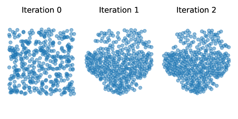
(a) Fixed-point iterations for $(p,q)=(\frac{3}{2},\frac{3}{2})$.

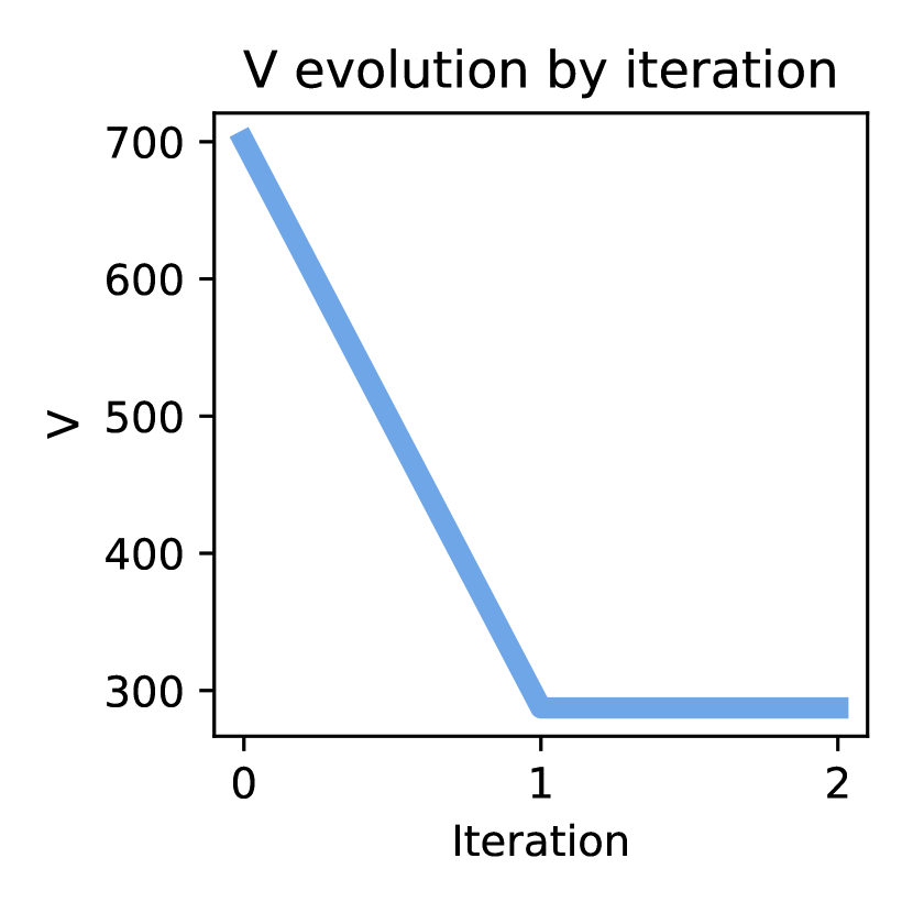
(b) Barycentre energy $V$ of the iterations.

Figure 6: Convergence of the fixed-point algorithm.

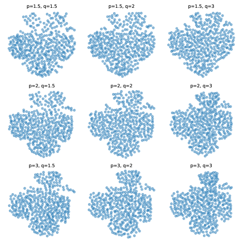
Figure 7: Barycentres for the cost $\|x-y\|_{p}^{q}$ for different values of $(p,q)$.

5.2 Comparison with the Multi-Marginal Formulation

Following Eq.˜7, the discrete OT barycentre problem has a multi-marginal formulation, which can be written as follows, given measures $\nu_{k}=\sum_{j=1}^{m_{k}}b_{k,j}\delta_{y_{k,j}}$:

$$\underset{\pi\in\Pi(b_{1},\cdots,b_{K})}{\operatorname{argmin}}\ \sum_{j_{1},\cdots,j_{K}}\pi_{j_{1},\cdots,j_{K}}\sum_{k=1}^{K}c_{k}(B(y_{1,j_{1}},\cdots,y_{K,j_{K}}),y_{k,j_{k}}).$$ (37)

Numerical solvers for Eq.˜37, while slow, allow the computation of the exact solution of the barycentre problem. Comparing this solution to the output of our algorithm is technical, since the barycentric version of our algorithm imposes the size of the support of the barycentre in addition to imposing the weights, which introduces bias. We aim to illustrate that the speed of the barycentric algorithm, with a quantitative study of the error with respect to the multi-marginal "ground truth". Note that even in this square-euclidean experiment, there is no widespread multi-marginal solver, which is why we also contribute an implementation.

The experimental setup is the following: the $K$ measures $\nu_{k}$ are all uniform measures with $n$ points in $\mathbb{R}^{d}$ drawn independently from $\mathcal{N}(0,1)$. For the fixed-point algorithm, the initial measure is also taken as a uniform measure over $n$ points with $\mathcal{N}(0,1)$ samples. We compare different numbers of iterations of the fixed-point algorithm and different choices of $n,d,K$. The plots show the ratios of the energy $V$ and computation times for our algorithm divided by a Linear Programming multi-marginal solver, plotting 30% and 70% quantiles across 10 samples for each configuration.

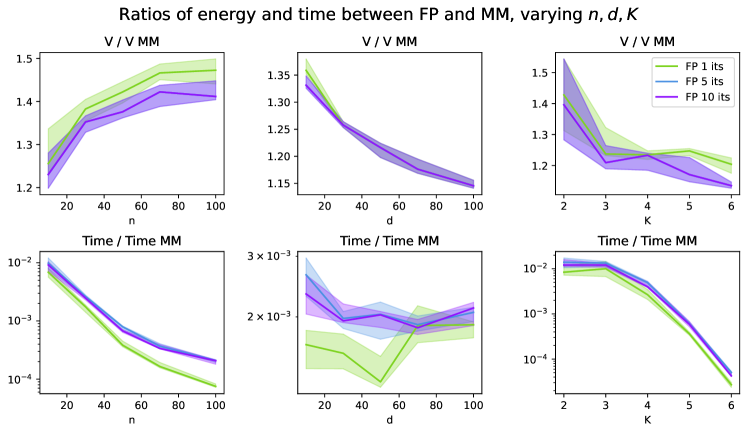
Figure 8: Comparing the fixed-point solver with a linear programming multi-marginal solver. From left to right columns: varying $n$ with $d=10$ and $K=3$; varying $d$ with $n=30$ and $K=3$; varying $K$ with $n=10$ and $d=10$. The comparison is made by dividing the energy value $V$ (resp. computation time) of the fixed-point solution by the multi-marginal solution. The different curves correspond to $T=1,5,10$ iterations (legend in the top-right).

From the results presented in Fig.˜8, it appears that the fixed-point algorithm converges in very few iterations, has an energy at most 50% worse than the exact multi-marginal solution, and is orders of magnitude faster, especially for larger measure sizes $n$ and for greater numbers of marginals $K$. Note that for $n\geq 10$ and $K\geq 10$ for example, the multi-marginal problem is computationally intractable.

To compare with similar barycentre support sizes, in Fig.˜9 we experiment with fixed-point barycentres with $N_{\mathrm{FP}}=(n-1)K+1$ points. The rationale behind this choice stems from the fact that discrete measures with $n_{1},\cdots,n_{K}$ points have a barycentre with at most $\sum_{k}n_{k}-K+1$ points ([7] Theorem 2.).

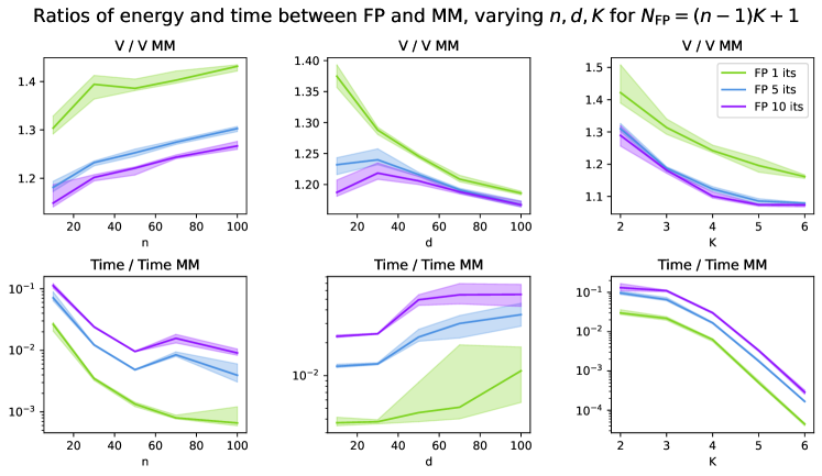
Figure 9: Comparing the fixed-point solver for $N_{\mathrm{FP}}=(n-1)K+1$ and the same setup as in Fig.˜8.

Comparing Figs.˜8 and 9 suggests that the fixed-point method is useful as a fast approximate solver for the barycentre problem, and that settings with larger barycentre supports may require more iterations to converge. The main takeaway is that our method remains competitive for large supports (comparable to the multi-marginal solution), yet its convergence speed and overall advantages are more pronounced for smaller supports (comparable to the supports of the marginals).

5.3 Generalised Wasserstein Barycentre Computation

In Fig.˜10(a), we illustrate the case where $c_{k}(x,y)=\|P_{k}x-y\|_{2}$, where $P_{k}:\mathbb{R}^{3}\longrightarrow\mathbb{R}^{2}$ is an orthogonal projection. The problem finds a 3D measure whose projections attempt to match the reference 2D measures, which we compare in Fig.˜10(b). This is a modification of the exponent 2 from Generalised Wasserstein Barycentres [21].

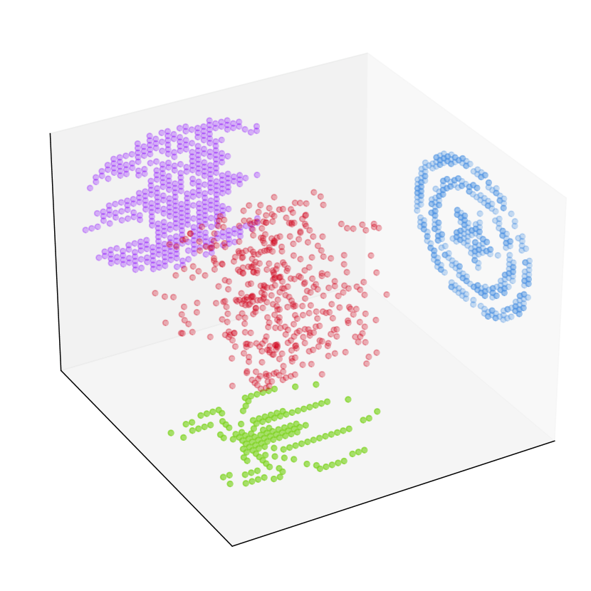
(a) Barycentre in $\mathbb{R}^{3}$ with immersed measures $\nu_{k}\in\mathcal{P}(\mathbb{R}^{2})$.

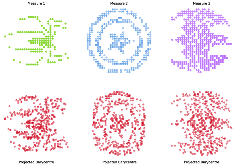
(b) Projections of the barycentre into $\mathbb{R}^{2}$.

Figure 10: Barycenter with costs $c_{k}(x,y)=\|P_{k}x-y\|_{2}$, where $P_{k}$ are orthogonal projections from $\mathbb{R}^{3}$ to the three axes-aligned planes of the orthonormal basis. We provide an animation in the companion code.

5.4 Non-linear Generalised Wasserstein Barycentre Computation

In this illustration, we look for a barycentre in $\mathbb{R}^{2}$ whose projections onto different circles match measures on these circles. We choose the costs $c_{k}(x,y)=\|P_{k}(x)-y\|_{2}^{2}$, where $P_{k}$ is the projection onto the circle $k$. Since $P_{k}$ is not linear, this is a direct generalisation of [21].

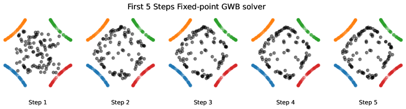
Figure 11: First 5 iterations of the fixed-point algorithm for costs $c_{k}(x,y)=\|P_{k}(x)-y\|_{2}^{2}$, where $P_{k}$ are projections onto four different circles on which the $\nu_{k}$ are supported (plotted in colour).

In this instance, convergence happens quickly, but a stationary point is only reached after about 5 iterations, as observed on the steps in Fig.˜11 and on the energy curve in Fig.˜12.

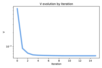
Figure 12: Barycentre energy $V$ of the fixed-point algorithm across iterations.

5.5 Gaussian Mixture Model Barycentres

We illustrate numerical solutions of the GMM Barycentre method introduced in Section˜4.4. In Fig.˜13, we compare the multi-marginal solution with the output of our algorithm.

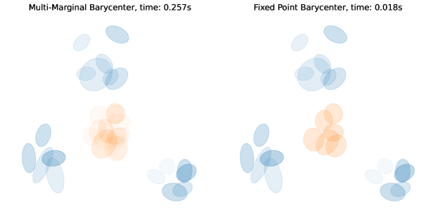
Figure 13: Left: multi-marginal solution for the GMM barycentre problem. Right: fixed-point solution for $n=6$ components.

Finally, in Fig.˜15 we illustrate barycentres between 4 GMMs shown in Fig.˜14 with different weights.

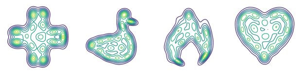
Figure 14: Four GMMs of which we will compute barycentres in Fig.˜15.

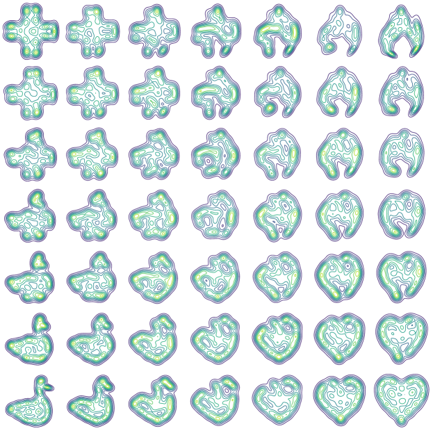
Figure 15: GMM barycentres between the four corner GMMs computed with the fixed-point solver with $n=15$ components. The GMMs are represented by the contours of their densities on $\mathbb{R}^{2}$.

Future Directions

There are numerous directions for future research. To begin with, in Theorems˜3.10 and 3.13, we show subsequential convergence to fixed-points of $G$ (resp. $G_{\varepsilon}$), which may not be barycentres. In cases where barycentres and fixed points may not be unique such as the discrete setting, it remains unclear if there exists fixed points that are not barycentres.

The barycentric fixed-point algorithm (iterating Eq.˜21) has no theoretical guarantees of convergence. Given its computational advantages and its current use in practice for the squared Euclidean cost ([19], [22]), this is a timely question.

In Section˜3.3, we required a notion of barycentric projection for couplings $\pi\in\Pi_{c_{k}}^{*}(\mu,\nu_{k})$. In $\mathbb{R}^{d}$, the underlying convex combinations are performed using the usual linear structure, however this does not generalise to arbitrary metric spaces. To consider these object more formally on generic (compact) metric spaces, it would be necessary to discuss in more detail the meaning of expectation in a space without a linear structure.

Throughout this work, we relied heavily on ˜2, but in practice this can be difficult to verify for costs $c_{k}$: beyond the case $c_{k}=h(x-y)$ with $h$ strictly convex, it is difficult to provide large classes of costs that yield this property on $B$ (other examples include $c_{k}(x,y)=\|P_{k}x-y\|_{2}^{2}$ as in [21] or $\mathrm{W}_{2}^{2}$ for absolutely continuous measures). One could alternatively investigate a theoretical framework where $B$ is a multi-function.

In the absolutely continuous case, the Twist condition can ensure uniqueness of the barycentre, as explained in Remark˜2.1. A natural question concerns almost-sure uniqueness in the discrete case, as was partially explored in Section˜4.3.

From a numerical standpoint, it has been observed that the fixed-point algorithm converges in very few iterations. A theoretical work extending the discrete Wasserstein case from [28] would bridge a significant gap between theory and practical observation.

Acknowledgements

We would like to thank Christophe Gaillac for the initial discussions that motivated the introduction of barycentres with generic costs. This research was funded in part by the Agence nationale de la recherche (ANR), Grant ANR-23-CE40-0017 and by the France 2030 program, with the reference ANR-23-PEIA-0004.

References

- [1] Martial Agueh and Guillaume Carlier. Barycenters in the Wasserstein space. SIAM Journal on Mathematical Analysis, 43(2):904–924, 2011.
- [2] Martial Agueh and Guillaume Carlier. Vers un théorème de la limite centrale dans l’espace de wasserstein? Comptes Rendus. Mathématique, 355(7):812–818, 2017.
- [3] Charalambos D. Aliprantis and Kim C. Border. Correspondences, pages 458–520. Springer Berlin Heidelberg, Berlin, Heidelberg, 1994.
- [4] Jason Altschuler, Sinho Chewi, Patrik R Gerber, and Austin Stromme. Averaging on the bures-wasserstein manifold: dimension-free convergence of gradient descent. Advances in Neural Information Processing Systems, 34:22132–22145, 2021.
- [5] Jason M. Altschuler and Enric Boix-Adsera. Wasserstein barycenters are np-hard to compute, 2021.
- [6] Pedro C Álvarez-Esteban, E Del Barrio, JA Cuesta-Albertos, and C Matrán. A fixed-point approach to barycenters in Wasserstein space. Journal of Mathematical Analysis and Applications, 441(2):744–762, 2016.
- [7] Ethan Anderes, Steffen Borgwardt, and Jacob Miller. Discrete Wasserstein barycenters: Optimal transport for discrete data. Mathematical Methods of Operations Research, 84:389–409, 2016.
- [8] Julio Backhoff-Veraguas, Joaquin Fontbona, Gonzalo Rios, and Felipe Tobar. Bayesian learning with wasserstein barycenters. ESAIM: Probability and Statistics, 26:436–472, 2022.
- [9] Florian Beier and Robert Beinert. Tangential fixpoint iterations for gromov-wasserstein barycenters, 2024.
- [10] Florian Beier, Robert Beinert, and Gabriele Steidl. Multi-marginal gromov-wasserstein transport and barycenters, 2023.
- [11] Jean-David Benamou, Guillaume Carlier, Marco Cuturi, Luca Nenna, and Gabriel Peyré. Iterative bregman projections for regularized transportation problems. SIAM Journal on Scientific Computing, 37(2):A1111–A1138, 2015.
- [12] Rajendra Bhatia, Tanvi Jain, and Yongdo Lim. On the Bures-Wasserstein distance between positive definite matrices. arXiv, December 2017.
- [13] Jérémie Bigot, Elsa Cazelles, and Nicolas Papadakis. Penalization of barycenters in the wasserstein space. SIAM Journal on Mathematical Analysis, 51(3):2261–2285, 2019.
- [14] Nicolas Bonneel, Gabriel Peyré, and Marco Cuturi. Wasserstein barycentric coordinates: histogram regression using optimal transport. ACM Trans. Graph., 35(4):71–1, 2016.
- [15] Camilla Brizzi, Gero Friesecke, and Tobias Ried. -Wasserstein barycenters, 2024.
- [16] Camilla Brizzi, Gero Friesecke, and Tobias Ried. -Wasserstein barycenters. arXiv preprint arXiv:2405.09381, 2024.
- [17] Guillaume Carlier, Enis Chenchene, and Katharina Eichinger. Wasserstein medians: Robustness, pde characterization, and numerics. SIAM Journal on Mathematical Analysis, 56(5):6483–6520, 2024.
- [18] Guillaume Carlier and Ivar Ekeland. Matching for teams. Economic theory, 42:397–418, 2010.
- [19] Marco Cuturi and Arnaud Doucet. Fast computation of Wasserstein barycenters. In Eric P. Xing and Tony Jebara, editors, Proceedings of the 31st International Conference on Machine Learning, volume 32 of Proceedings of Machine Learning Research, pages 685–693, Bejing, China, 22–24 Jun 2014. PMLR.
- [20] Julie Delon and Agnes Desolneux. A Wasserstein-type distance in the space of gaussian mixture models. SIAM Journal on Imaging Sciences, 13(2):936–970, 2020.
- [21] Julie Delon, Nathaël Gozlan, and Alexandre Saint-Dizier. Generalized Wasserstein barycenters between probability measures living on different subspaces, 2021.
- [22] Rémi Flamary, Nicolas Courty, Alexandre Gramfort, Mokhtar Z. Alaya, Aurélie Boisbunon, Stanislas Chambon, Laetitia Chapel, Adrien Corenflos, Kilian Fatras, Nemo Fournier, Léo Gautheron, Nathalie T.H. Gayraud, Hicham Janati, Alain Rakotomamonjy, Ievgen Redko, Antoine Rolet, Antony Schutz, Vivien Seguy, Danica J. Sutherland, Romain Tavenard, Alexander Tong, and Titouan Vayer. POT: Python optimal transport. Journal of Machine Learning Research, 22(78):1–8, 2021.
- [23] Promit Ghosal, Marcel Nutz, and Espen Bernton. Stability of entropic optimal transport and schrödinger bridges. Journal of Functional Analysis, 283(9):109622, 2022.
- [24] Paula Gordaliza, Eustasio Del Barrio, Gamboa Fabrice, and Jean-Michel Loubes. Obtaining fairness using optimal transport theory. In International conference on machine learning, pages 2357–2365. PMLR, 2019.
- [25] Nhat Ho, XuanLong Nguyen, Mikhail Yurochkin, Hung Hai Bui, Viet Huynh, and Dinh Phung. Multilevel clustering via wasserstein means. In International conference on machine learning, pages 1501–1509. PMLR, 2017.
- [26] Young-Heon Kim and Brendan Pass. Wasserstein barycenters over Riemannian manifolds. Adv. Math., 307:640–683, 2017.
- [27] Alexander Korotin, Vage Egiazarian, Lingxiao Li, and Evgeny Burnaev. Wasserstein iterative networks for barycenter estimation. Advances in Neural Information Processing Systems, 35:15672–15686, 2022.
- [28] Johannes von Lindheim. Simple approximative algorithms for free-support Wasserstein barycenters. Computational Optimization and Applications, 85(1):213–246, 2023.
- [29] Quentin Mérigot, Alex Delalande, and Frederic Chazal. Quantitative stability of optimal transport maps and linearization of the 2-Wasserstein space. In International Conference on Artificial Intelligence and Statistics, pages 3186–3196. PMLR, 2020.
- [30] Liang Mi, Wen Zhang, Xianfeng Gu, and Yalin Wang. Variational wasserstein clustering. In Proceedings of the European Conference on Computer Vision (ECCV), pages 322–337, 2018.
- [31] Eduardo Fernandes Montesuma and Fred Maurice Ngole Mboula. Wasserstein barycenter for multi-source domain adaptation. In Proceedings of the IEEE/CVF conference on computer vision and pattern recognition, pages 16785–16793, 2021.
- [32] G. Peyré and M. Cuturi. Computational optimal transport. Foundations and Trends in Machine Learning, 51(1):1–44, 2019.
- [33] Yury Polyanskiy and Yihong Wu. Lecture notes on information theory. Lecture Notes for ECE563 (UIUC) and, 6(2012-2016):7, 2014.
- [34] Julien Rabin, Gabriel Peyré, Julie Delon, and Marc Bernot. Wasserstein barycenter and its application to texture mixing. In Scale Space and Variational Methods in Computer Vision: Third International Conference, SSVM 2011, Ein-Gedi, Israel, May 29–June 2, 2011, Revised Selected Papers 3, pages 435–446. Springer, 2012.
- [35] Filippo Santambrogio. Optimal transport for applied mathematicians. Birkäuser, NY, 55(58-63):94, 2015.
- [36] Justin Solomon, Fernando De Goes, Gabriel Peyré, Marco Cuturi, Adrian Butscher, Andy Nguyen, Tao Du, and Leonidas Guibas. Convolutional wasserstein distances: Efficient optimal transportation on geometric domains. ACM Transactions on Graphics (ToG), 34(4):1–11, 2015.
- [37] Cédric Villani. Optimal transport : old and new / Cédric Villani. Grundlehren der mathematischen Wissenschaften. Springer, Berlin, 2009.