Adaptive Algebraic Reuse of Reordering in Cholesky Factorization with Dynamic Sparsity Pattern
Abstract.
Cholesky linear solvers are a critical bottleneck in a wide range of challenging applications within computer graphics and scientific computing. These applications include, but are not limited to, elastodynamic barrier methods such as Incremental Potential Contact (IPC), and geometric operations such as remeshing, and morphology. In these contexts, the sparsity patterns of the linear systems frequently change across successive calls to the Cholesky solver, necessitating repeated symbolic analyses that dominate the overall solver runtime.
To address this bottleneck, we evaluate our method on over 150,000 linear systems generated from diverse nonlinear problems with dynamic sparsity changes in Incremental Potential Contact (IPC) and Patch remeshing on a wide range of triangular meshes with various sizes. Our analysis using three leading sparse Cholesky libraries—Intel MKL Pardiso, SuiteSparse CHOLMOD, and Apple Accelerate—reveals that the primary performance constraint lies in the symbolic re-ordering phase of the solver. Recognizing this, we introduce Parth, an innovative re-ordering method designed to update ordering vectors only where local connectivity changes occur adaptively. Parth employs a novel hierarchical graph decomposition algorithm to break down the dual graph of the input matrix into fine-grained subgraphs, facilitating the selective reuse of fill-reducing orderings when sparsity patterns exhibit temporal coherence.
Our extensive evaluation demonstrates that Parth achieves up to a 255× and 13x speedup in fill-reducing ordering for our IPC and remeshing benchmark and a 6.85x and 10.7x acceleration in symbolic analysis. These enhancements translate to up to 2.95x and 5.89x reduction in overall solver runtime. Additionally, Parth’s integration requires only three lines of code, resulting in significant computational savings without the requirement of change in the computational stack. By providing a comprehensive analysis of Parth’s performance across various solvers and applications, we enable practitioners to make informed decisions about their linear solver choice tailored to their specific computational workflows. We hope that Parth facilitates faster and more scalable solutions in dynamic and complex computational environments.
1. Introduction
Linear solvers lie at the heart of many applications in graphics and scientific computing. Due to the structure induced by mesh-based computations, many common operations such as solving partial differential equations or minimizing a variational energy give rise to sparse systems of linear equations – for the solution of which, it is either necessary or convenient to rely on Cholesky solvers. As a result, their accelerations are well-studied. However, the runtime of graphic applications often remain dominated by the cost of Cholesky solves, necessitating their further acceleration.
Efficient sparse Cholesky solvers are typically designed with static sparsity patterns in mind. The solution procedure itself is divided into two steps: ”symbolic analysis,” where the sparsity pattern of the matrix representing the system of linear equations is analyzed, and ”numerical computation,” which uses the symbolic analysis information to efficiently compute the solution. Often, a single symbolic analysis requires more computational resources than a single numerical computation (see Section 5). In cases of fixed sparsity, repeated solves can be accelerated by caching and reusing the results of a single symbolic computation. However, in applications with changing sparsity patterns, this optimization is unavailable.
In this work, we focus on optimizing the performance of Cholesky solvers in applications with temporally-coherent, local changes in sparsity pattern, such as those observed in contact simulation with elasticity (Li et al., 2020) and geometric operations with remeshing including mapping (Schmidt et al., 2023) and morphology (Sellán et al., 2020) in their computational pipeline. In such applications, the overhead of repeated symbolic analyses becomes the bottleneck of linear solve costs. For example, in our evaluation of Incremental Potential Contact (IPC) (Li et al., 2020), we see that symbolic analysis accounts for up to 78% of the total runtime of the Cholesky solver. Also, in our evaluation of patch remeshing pipeline (see Section 17), we observe that 82% of the total runtime of Cholesky solver is spend on symbolic analysis. In this work, we leverage temporal coherence in sparsity patterns, common in graphics workflows, to adaptively reuse prior symbolic analysis to accelerate sparse Cholesky solves.
Our main contribution is Parth, an adaptive and general algorithm that enables reuse in symbolic analysis across repeated Choleksy solves when changes in the sparsity pattern are localized and temporally consistent. Parth has two key objectives: (I) adaptive reuse focused on changing linear-system sparsity structure, and (II) general-purpose, practical integration across high-performance Cholesky solver packages and libraries. The first provides generality and portability across diverse applications, while the second enables speed-ups with the state-of-the-art reliable and performant Cholesky solvers.
We evaluate well over 150 thousand linear solves from challenging physics simulations and geometric processing problems with dynamic sparsity patterns. We first identify symbolic analysis as a primary bottleneck in these applications. Within symbolic analysis, we then pinpoint fill-reducing ordering as the bottleneck of the process. Symbolic analysis provides a permutation that minimizes fill-ins during Cholesky solve computation (Davis et al., 2016). Consequently, this paper specifically focuses on a set of algorithms for adaptive reuse of fill-reducing ordering computations.
Integrating Parth into high-performance Cholesky solvers—Apple Accelerate (Inc., 2023), Intel MKL (Schenk et al., 2001), and CHOLMOD (Chen et al., 2008)—and evaluating them on our two benchmarks, IPC and Remeshing, we observe up to a 255× and 13× speedup in fill-reducing ordering performance, respectively. These improvements result in a 6.85× and 10.7× speedup in symbolic analysis performance. Consequently, these enhancements translate into up to a 2.95× and 5.89× speedup in the per-solve Cholesky computation, respectively (refer to Section 5 for more details). Additionally, we demonstrate that by adding the three lines of code required to integrate Parth into the Cholesky solve computational pipeline of our IPC benchmark (see Section 5.2), our most challenging simulation (“Arma Roller”) achieves seven hours less computational time with only a 1.5× speedup in the total Cholesky solve runtime, without any side effects on numerical performance. Finally, recognizing that different graphical computational pipelines may exhibit varying behaviours in gradual reuse, we provide a per-solve analysis of Parth’s effects. This analysis demonstrates different reuse scenarios, including local changes in single and multiple locations, as well as varying sizes of changes in both the number of rows/columns and the non-zero entries of the matrix. These insights allow practitioners to understand how Parth performs in their specific applications.
Our technical contributions enabling this reuse are: (I) A novel hierarchical graph decomposition algorithm that decomposes the graph dual of the input matrix—representing the sparsity pattern of the system of linear equations—into multiple fine-grain sub-graphs. (II) To leverage the hierarchical characteristics of the decomposition, we propose a new algorithm that confines changes to fine- or coarse-grain sub-graphs, enabling reuse in static parts of the graph. (III) Finally, we provide an extensive evaluation of high-performance Cholesky solvers in dynamic scenarios, where the sparsity pattern changes due to different non-zero entries, as well as changes caused by modifications to the number of rows/columns of the matrix. To our knowledge, this thorough analysis is not currently available, allowing practitioners to make informed choices for their Cholesky solver baselines and computational pipelines.
In summary, we present Parth, a method that reuses symbolic information in the presence of dynamic sparsity patterns with temporal coherence across calls to the Cholesky solver. We evaluate Parth’s performance across a wide range of different solve scenarios. We focus on three highest-performing Cholesky solvers—CHOLMOD (Chen et al., 2008), the recently developed Apple Accelerate sparse kernels (Inc., 2023), and Intel MKL (Schenk et al., 2001) 111We choose these by also comparing them with alternate available solvers, Sympiler (Cheshmi et al., 2017), Parsy (Cheshmi et al., 2018a), and Eigen (Liu et al., 2021). See Appendix F. We hope that our extensive analysis not only provides insight into how Parth improves performance for these tools across the board but also into the specifics of each of these state-of-the-art Cholesky solvers’ performance. Together these will help practitioners to make informed application-specific decisions for which framework to use based on our presented comprehensive quantitative comparison.
2. Related Work
Enhancing the performance of Cholesky factorizations and Sparse Triangular Solves (SpTRSV), remain a significant focus in computational mathematics and computer graphics due to their critical roles in simulation and optimization problems.
Exploiting Dense Computation: Early optimizations center on exploiting dense computations within sparse factorizations.Liu (1990) utilize the elimination tree to create supernode—groups of consecutive rows/columns sharing the same sparsity pattern. These supernodes are then factorized using dense BLAS(Dongarra et al., 1990) kernels, enhancing computational efficiency by leveraging optimized dense linear algebra routines. Subsequent methods, such as CHOLMOD (Chen et al., 2008), relax strict supernode constraints, allowing for better trade-offs by utilizing dense computation more effectively. These come at the expense of more redundant computation by increasing the size of the supernodes even when some rows/columns do not have a matching pattern.
Parallelism and Scheduling Algorithms: While initial focus was primarily on finding dense computations within the chaos of sparse computations, later work focuses on further enabling parallelism across the computation of these dense blocks. This led to the introduction of advanced scheduling algorithms that balance load across parallel units, optimize memory usage through data reuse, and reduce synchronization overhead. MKL PARDISO (Schenk et al., 2001) improves parallelism by efficiently distributing tasks across multiple cores and handling thread-level parallelism. Load-Balancing Coarsening (LBC)(Cheshmi et al., 2018b) enhances memory usage by improving data locality and minimizing cache misses during computation on CPUs, as the parallelism of Cholesky factorization is limited by the sparsity pattern, and memory reuse can provide some compensation for the lack of parallelism. Additionally, the CHOLMOD GPU scheduler(Rennich et al., 2016) targets GPU hardware to achieve significant speedups in numerical computation, achieving up to a 2x speedup compared to CPU implementations.
Code Generation: Recent approaches focus on providing optimized code by inspecting the sparsity pattern during symbolic analysis to improve numerical computation efficiency. Sympiler (Cheshmi et al., 2017) analyzes sparsity patterns to generate specialized, pattern-specific code that optimizes memory access and computational efficiency. Similarly, Cheshmi et al. (2023) automates the generation of high-performance code for sparse applications by fusing kernels used in linear solvers. However, this analysis comes with a high overhead of inspection, which further increases symbolic analysis overhead and must be redone if the sparsity pattern changes.
Reuse of Numerical Factorization: Efforts to reuse numerical factorization in linear solve computations aim to reduce the costs associated with recomputing factors for systems with numerical temporal coherence. In Davis and Hager (2005), a method for reusing factors via low-rank updates is introduced. Li et al. (2021) extend this work to support low-rank updates in the presence of dynamic sparsity patterns. However, as they mention in their paper, this method does not perform well when multiple local changes occur in the sparsity pattern, and they can not reuse symbolic analysis in such cases. Another body of work on reusing factorization computation is proposed in (Herholz and Alexa, 2018; Herholz and Sorkine-Hornung, 2020), where a prior factor is reused across calls to the linear solver by only recomputing the affected supernodes. However, these methods often introduce approximation errors, limiting their applicability in contexts where the precision of Cholesky solvers is essential. Furthermore, they can not be applied to applications with dynamic sparsity patterns, as the elimination tree structure relies on changes across calls to Cholesky solvers, leading to the reconstruction of supernodes. NASOQ (Cheshmi et al., 2020) provides a constraint-based QP solver that reuses factorization computation across calls to a constraint-based QP solver, as adding and removing these constraints requires a factorization. To handle changes in the sparsity pattern due to changes in constraints, it performs a full symbolic analysis with all possible constraints added and uses a subset of the symbolic analysis when the constraints are added or removed from the KKT matrix. However, this approach assumes prior knowledge of all potential constraints and can not handle new sparsity patterns not known in advance.
In contrast to existing methods, our work focuses on reusing symbolic analysis instead of numerical factorization to address the overhead caused by dynamic sparsity patterns in Cholesky factorization. Specifically, we assume no prior knowledge of where changes may occur or how many changes can happen across each call to the Cholesky solver. By developing algorithms that identify and reuse unchanged portions of the symbolic analysis across iterations, we significantly reduce the overhead associated with the symbolic phase. This approach effectively handles multiple local changes while providing high-quality fill-reducing ordering.
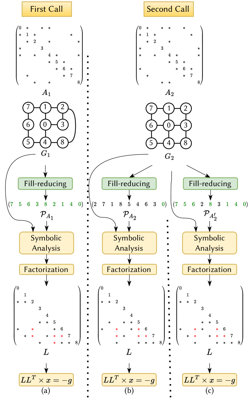
Cholesky solver computational pipeline for two calls. The difference between columns 0,2, and 3 between the first and second calls requires the computation of a fill-reducing vector in both calls. As shown in sub-figures (b) and (c) which process the same matrix, one can see that two permutation vectors produce identical fill-in counts. However, Figure 2(c) displays an ordering vector, , that is more similar to , as shown by the values coloured green, especially when contrasted with Figure 2(b). This similarity shows the potential for computational reuse of fill-reducing orderings while providing a high-quality permutation vector.
3. Background
Solving the fill-reducing ordering problem is NP-hard (Yannakakis, 1981). However, commercial Cholesky linear solvers apply well-tested heuristic-based methods such as METIS (Karypis and Kumar, 1997), AMD (Amestoy et al., 2004) and Scotch (Pellegrini, 2009) that provide high-quality fill-reducing orderings. These algorithms incorporate randomness in their routines, resulting in multiple fill-reducing orderings for a single input, highlighting the existence of multiple possible high-quality orderings for a given linear system. Parth introduces a method that finds a high-quality fill-reducing ordering by reusing computations from previous calls to the ordering module. As an example, in Figure 2, two systems of linear equations with gradual changes can produce multiple high-quality permutation vectors, where one of these ordering vectors has high similarity to the previous call indicating the existence of a solution while reusing the computation from the previous call.
Parth achieves this by operating on the graph dual of the system of linear equations , rather than directly analyzing application-specific properties. In particular, for a system of linear equations , where is symmetric, the matrix can be viewed as an adjacency matrix. In this view, each row/column corresponds to a node in graph , and non-zero entries define the edges between nodes. This approach makes Parth general, as could represent, for example, a Laplace-Beltrami operator or the Hessian of an energy function constructed for a Newton iteration solve. Additionally, fill-reducing ordering algorithms also use the graph dual of the input matrix , aligning Parth’s computational pipeline with that of a general high-performance Cholesky solver. An example of graph duals and for and matrices is shown in Figure 2. Note that the graph dual does not consider diagonal entries of .
While the input Parth considers is general, the heuristics applied by Parth are based on an abstract connection between the graph and an underlying application’s degrees of freedom (DOF) and evaluation stencils. For instance, many geometric processing applications utilize cotangent Laplace-Beltrami operators where the nodes in the graph can represent DOF, and the edges correspond to the stencils formed by elements in the mesh. For Hessian formed by the Incremental Potential Contact (IPC) (Li et al., 2020) method, each set of three consecutive rows in Hessian represent the properties of the x, y and z directions of a single DOF. This abstract connection - linking the mesh to the graph dual of - provides us with a geometric connection that is considered in Parth algorithms. Consequently, while our approach may apply to other scenarios, as we aim to be as general as possible, this work focuses on mesh-based computations where the relationship between the graph and the underlying application, as described, is key.
The following section explains Parth’s modules, which efficiently produce high-quality fill-reducing ordering vectors by reusing computation, requiring only the addition of three lines of code to add it to pre-existing Cholesky linear solver pipelines.
4. Parth Framework
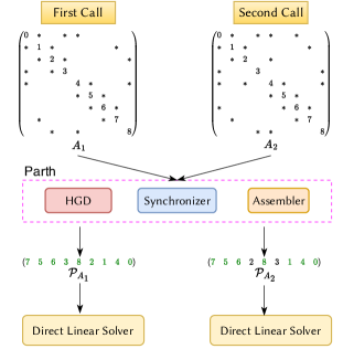
Figure 3 illustrates Parth’s integration into high-performance Cholesky solver libraries for solving the two calls to the Cholesky solver for the problem described in Figure 2. As shown, Parth replaces the fill-reducing module of high-performance Cholesky solvers and provides its own permutation vector to these tools. In the following, we explain the internal modules of Parth, followed by its input and output to present the computational pipeline that enables the reuse of fill-reducing ordering computation.
Parth’s Modules: Figure 3 shows the three underlying modules of Parth. The Hierarchical Graph Decomposition (HGD) algorithm decomposes the dual graph of the system of linear equations into multiple smaller sub-graphs (fine-grain) that can be coarsened to form larger sub-graphs (coarse-grain). Furthermore, the decomposition enables the creation and combination of local permutation vectors per sub-graph. A Synchronizer module detects and integrates sparsity pattern changes into the created sub-graphs, thereby localizing the effects of these changes by confining them to specific coarse- or fine-grain sub-graphs. The Assembler unit then reuses the local permutation vectors in unchanged sub-graphs and updates those that are changed, finally assembling all this information into a single permutation vector, .
Input: As shown in Figure 3, Parth’s input is matrix . The graph dual, as shown in Figure 2, simply uses as an adjacency matrix (without its diagonal entries). If the user specifies that, for example, every three consecutive rows in the form of represent the properties of a single node and are fully coupled, Parth can coarsen the graph and use that for analysis, as these terms are fully coupled, and this compression does not affect the quality of fill-reducing ordering. This process is explained in more detail in Section 4.3.
Output: Parth’s output is a permutation vector applicable to matrix . The permutation vector generated in the second call shares seven identical entries with the permutation vector in the first call. This is due to Parth’s mechanism, which reuses the permutation vector information from the first call. By updating only the necessary local permutation vectors and integrating the updated information into , the permutation vector has far more similarity to previous vector, than a conventional fill-reducing algorithm. By reusing the information, Parth enhances the performance of fill-reducing ordering computation by up to 255x speedup per frame in our IPC benchmark.
This performance can be easily provided to practitioners, as many commercial Cholesky solvers such as Intel MKL, CHOLMOD, or Apple Accelerate accept user-provided fill-reducing orderings. When such an interface exists, the fast fill-reducing orderings computed by Parth can be directly supplied, increasing the performance of these off-the-shelf tools without any modification to the underlying source code.
4.1. Parth: Hierarchical Graph Decomposition
The Hierarchical Graph Decomposition (HGD) algorithm is designed to encapsulate changes within sub-graphs. Changes in the sparsity pattern due to, for example, contact during a simulation or re-meshing are reflected in changes in the graph dual . The Hierarchical Graph Decomposition module (HGD) attempts to encapsulate those changes within local sub-graphs to facilitate local updates to the fill-reducing ordering.
To accomplish this, HGD’s decomposition uses a separator set computation which is also used in nested dissection algorithms. As a variant of this algorithm is employed in METIS, a well-known fill-reducing ordering algorithm, Parth can reuse this computation as part of the fill-reducing ordering process. HGD encodes the decomposed graph information into a binary tree. This representation enables Parth to provide both fine and coarse-grained subgraphs simultaneously, allowing for encompassing changes in arbitrary places with negligible overhead when compared to the computation of fill-reducing ordering itself.
Algorithm 1 shows the details of this process. Parth uses the HGD algorithm to iteratively construct a binary tree data structure, , stored as an array. The total number of nodes in the binary tree is computed using the maximum level in the binary tree. A level is defined as the distance between the node and the root. Thus, HGD uses the variable as the termination condition (line 1) for the recursion. Each call to the HGD algorithm results in a new binary tree node, represented as . Each binary tree node corresponds to a sub-graph within the graph-dual of . These subsets are determined by the recursive use of the function (line 2). Note that this function divides the graph into three distinct sub-graph: a separator set, , and two other sub-graphs, and . The separator set acts as a minimal sub-graph that, when removed, dissects the remaining graph into two nearly equal parts, ensuring a balance in size between and .
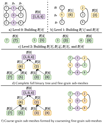
As an example, Figure 4 shows the HGD evaluation on from the ”First Call” in Figure 3. Figures 4(a-c) present the HGD process at three levels. Initially, the root node of the binary tree is created, shown as . The decomposition then recursively advances to levels 1 and 2, resulting in the creation of 2 and 4 additional nodes within . Each node in represents the smallest sub-graph in our decomposition. The final full binary tree is described in Figure 4(d). Note that each leaf of this binary tree represents a separate, approximately equal-sized sub-graph. The intermediate nodes in the binary tree are the separators, which also form part of the sub-graphs. This methodology effectively allows for coarsening sub-graphs by merging each sibling with its corresponding separator. Note that the coarsening can continue until all the sub-graphs are merged into the root, forming the whole . This demonstrates the hierarchical nature of the decomposition.
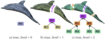
Note that in this toy example, the size of separator set is comparable even bigger that the size of the left and right sub-graphs. However, in real-world graphs drived from meshes, this is not the case. As an example, see Figure 5 where the binary tree created due to HGD process and the corresponding separator and left and right sub-graphs are shown for a dolphin mesh.
To further elaborate on why the HGD process has low overhead in practice, we provide details on the decomposition overhead as well as the size of the generated binary tree. The initial decomposition imposes an initialization overhead, and traversing the tree is a common task for providing fill-reducing ordering with reuse. Demonstrating why these two processes have low overhead provides insight into why Parth, as a whole, is a low-overhead procedure.
Sub-graph Decomposition Overhead: The HGD process leverages the nested-dissection approach (Khaira et al., 1992) to create the sub-graphs. Parth reuses information related to the separator sets and their corresponding left and right sub-graphs for computing the ordering vector which result in lower-overhead. This approach hides the HGD cost within the fill-reducing ordering computation, as shown in Section 5. For an example of how this information is reused for fill-reducing ordering computation, see Appendix A.
Binary Tree Usage Overhead: In practice, Parth achieves reasonable reuse by using a small , regardless of the mesh resolution. This results in low overhead when traversing the binary tree. To understand why a small provides effective reuse, we examine the relationship between the size of and Parth’s reuse capability.
To elaborate, let us consider how much reuse Parth can provide when . Regardless of how Parth confines the changes, these changes occur either within fine-grain or coarse-grain sub-graphs. When , each leaf node of represents roughly 25% of the total graph (considering small separator sets). Consequently, Parth can confine changes to either a fine-grain sub-graph of size 25%, achieving 75% reuse on the unchanged sub-graph, or to coarser sub-graphs of sizes 50% or 100%, which are the only coarse sizes generated by . This results in discretized reuse levels of 75%, 50%, or 0% (where changes cannot be confined locally).
Increasing max_level to 3 produces fine-grain sub-graphs of size 12.5%, leading to maximum reuse levels of 87.5%, 75%, 62.5%, and so forth, down to 0%. Thus, max_level controls the granularity of reuse that Parth can provide. For instance, setting results in 128 leaf nodes, approximating fine-grain sub-graphs of less than 1% of the total graph size. This enables reuse granularity of less than 1%, regardless of the mesh resolution, meaning Parth’s reuse can exceed 99%, which is sufficient in practice. Additionally, the number of nodes in a full binary tree with is 255. Based on our analysis, traversing such a small tree incurs minimal overhead in practice.
Finally, note that coarsening sub-graphs using this binary tree model does not involve explicitly coarsening the nodes in . Instead, Parth treats a sub-tree in as a coarsened sub-graph. Specifically, a separator and its corresponding left and right sub-graphs are treated as a single coarse sub-graph. For example, in Figure 4(f), the coarse sub-graph is formed by coarsening and with their shared separator . This process does not create entirely new sub-graphs; instead, it represents coarser sub-graphs using mutual separators from the fine-grain sub-graphs. This can also be seen in Figure 5, which illustrates how the coarse-grain sub-graphs in Figure 4(b) (colored yellow) are formed by viewing the fine-grain sub-graphs and their common separators in Figure 4(c) (colored blue) as single coarse sub-graph.
4.2. Parth: Synchronizer
The Synchronizer module in Parth synchronizes the information between and across calls to the linear solver by identifying changes in and encapsulating them within the set of sub-graphs in . If necessary, it re-decomposes the sub-graphs affected by these changes, as their nodes’ connectivity may now differ. This allows Parth to preserve fill-reducing ordering information in sub-graphs that remain unchanged, enabling the reuse of this information. The Synchronizer achieves this through the five-step procedure outlined in Algorithm 2, explained as follows:
Step 1: Synchronizing the Added or Removed DOFs: The Synchronizer algorithm begins by analyzing changes in the number of nodes in the graph (line 2). If the nodes differ, it then examines the map input. The map array simply maps the index of nodes in the current call to the index of the same nodes in the previous call. For a detailed explanation of how Parth uses the map array to synchronize the added or removed nodes into , see Appendix B. In our experience, remeshers either create the map array explicitly in their underlying process or straightforwardly allow for its creation, as it is required for generating the faces and vertices metadata for (re)defining a mesh. Therefore, we hope this requirement is not too restrictive for other applications that could benefit from Parth.
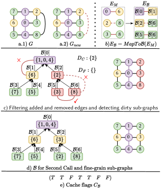
Step 2: Detecting Added or Removed Edges: The Synchronizer now identifies added or removed edges from the graph by comparing the current graph () with the previous one () (line 3). Note that for an added DOF, all the edges are considered new, and a removed DOF’s edges are not considered for computing the changed edges set . After this step, edges in are mapped to changes in , indicated by . To clarify, Figure 6(a) illustrates the detection of changes between the graph duals shown in Figure 3. The difference between the two sub-graphs includes the addition of edges <0,6>and <3,8>and the deletion of edge <2,8>. Additionally, these modifications are mapped to the connectivity changes between fine-grain sub-meshes represented by <, >, <, >, and <, >, as visualized in Figure 6(b).
Step 3: Detecting Dirty Sub-graphs: The Synchronizer module utilizes to identify sub-graphs affected by these changes. These affected sub-graphs, called ”dirty sub-graphs,” no longer possess valid information due to the changes. There are two categories of dirty sub-graphs: , which are fine-grain dirty sub-graphs, and , which are coarse-grain dirty sub-graphs (line 4). The distinction is made because fine-grain sub-graphs do not require re-decomposition; only their fill-reducing ordering information needs to be updated. In contrast, coarse-grain sub-graphs may experience a violation of the separator’s characteristics due to connectivity changes. That is, two sub-graphs that were supposed to be completely separated by a separator set are now connected via some nodes in the graph. Consequently, the Synchronizer must apply the HGD algorithm to re-decompose the coarse-grain regions and update the information as needed. For a detailed explanation of line 6 in the algorithm, see Appendix C.
To clarify the effect of the mentioned procedure, Figure 6(c) demonstrates the process of computing and using . The two changed edges <, >and <, >are disregarded because they do not disrupt the connection between the sub-graphs within the binary tree . For example, the change involving <, >is dismissed as the link between a separator and its adjacent left sub-graph does not violate the validity of the separator, given that separates from sub-graphs , , and . Conversely, the change involving <, >violates the separator’s role of , since the sub-graph now connects to sub-graph , resulting from the new connections between node 3 and node 8 in the graph. Consequently, the coarse sub-graph, annotated as and comprising simulation graph nodes , is added to as it encapsulates the change <3,8>.
Step 4: Filtering Sub-graphs: During the formation of and , each change is assessed independently from the others. As a result, some coarse-grained sub-graphs can encompass other fine- and coarse-grained sub-graphs. These smaller sub-graphs can subsequently be removed from and , as they will be re-decomposed when the larger, encompassing sub-graph is re-decomposed. After this stage, the coarse sub-graphs requiring re-decomposition are fully identified. For a real-world example, refer to Figure 7, where the contacts are restricted to a set of coarse sub-graphs (subsequently sub-meshes in the simulation mesh of IPC), colored in red, at the end of Step 4 (line 6 of Algorithm 2).
Step 5: Re-decomposing Sub-graphs: Finally, after the creation and filtering of and , the decomposition information in must be updated accordingly. For fine-grain sub-graphs in , we only need to mark them in the array so that the Assembler module (Section 4.3) updates the fill-reducing ordering information of these sub-graphs, as only the connectivity between the nodes has changed. For coarse-grain sub-graphs in , the Synchronizer first re-decomposes the sub-graphs using the HGD algorithm (Section 4.1). The newly formed fine-grain sub-graphs are then marked in for the computation of fill-reducing ordering. For a detailed explanation of the algorithm, see Appendix D.
As an illustration, on the right side of Figure 6(c), the Synchronizer initially extracts the coarse sub-graph, colored in red (nodes ). Given that the size of is constant, the Synchronizer is only required to substitute the invalid sub-graphs with valid ones. To achieve this, the process first identifies the sub-tree within that contains all the invalid sub-graphs (illustrated in red on the left side of Figure 6(c)). Next, it invokes the HGD algorithm on the sub-graph colored in red (Figure 6(c)-right) to produce a valid decomposition, which is then visualized as a new sub-tree. This new sub-tree is used to replace the invalidated one, resulting in a completely valid binary tree , as depicted in Figure 6(d). It is important to note that the sub-graph has been updated from the set to , which now effectively isolates sub-graph from sub-graph .
After updating the hierarchical graph decomposition, the new sub-graphs need the recomputation of fill-reducing ordering as the node structures they are representing have now changed. These dirty fine-grain sub-graphs are flagged within the array. For instance, Figure 6(e) indicates that the sub-graphs , , and are new and thus require updated fill-reducing information. As a result, both the array and the binary tree will be fed to the Assembler module for new fill-reducing ordering information.
As a final note, one of the drawbacks of this procedure is that a single edge connecting two sub-graphs with a common separator will result in the reuse of zero, as the coarse-grain sub-graph will encompass the whole graph. To alleviate this, we created a heuristic, explained in the Appendix D. The heuristic moves one of the nodes that form the problematic edge to the corresponding separator. That is, the sub-graph forming that separator will expand if this happens, allowing Parth to achieve high reuse even in these scenarios.
4.3. Parth: Assembler
The Assembler module generates the permutation vector by reusing computation across calls to Parth. Initially, the Assembler computes the required permutation vectors for each sub-graph represented by . It then assembles these local permutation vectors to form which applies to the whole matrix . Due to changes in sparsity pattern, if Synchronizer module marks some of the sub-graph ”dirty” (refer to Section 4.2), the Assembler computes a new local permutation vector for these ”dirty” sub-graphs. The values linked to these modified sub-graphs are then updated in , while the rest remain unchanged. This approach results in the computational reuse for all unchanged sub-graphs.
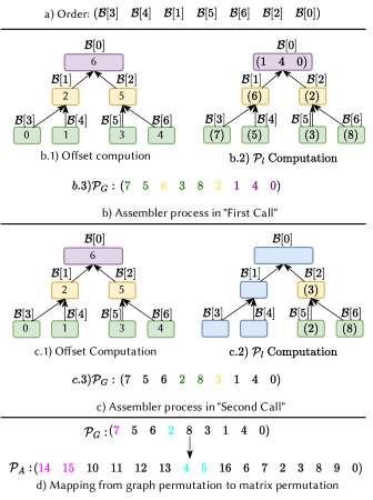
The Assembler procedure has three steps, as outlined in Algorithm 3. In Step 1, the procedure determines the placement of the local permutation vectors within . Step 2 involves the calculation of the necessary vectors which, using the previously computed positions from Step 1, are inserted into the . Finally, in Step 3, the graph permutation vector is converted into based on value. All three steps are capable of reusing pre-computed data based on the array , which indicates the affected sub-meshes. Details of these three steps are further explained as follows:
Step 1: Placement Computation: To use separators and their corresponding left and right sub-graphs as fill-reducing ordering information, we follow the nested-dissection approach. In this approach, the permutation vector is arranged in the computation so that the separator computation is placed after the left and right sub-graph computations (see Appendix A). Applying this order recursively is equal to placing each local permutation vector related to each node based on the post-order traversal of the tree. Consequently, the Assembler module creates the entire graph permutation vector . The Assembler executes this procedure in Lines 1-11 of Algorithm 3.
Looking at Figure 8, the post-order is computed once in Figure 8(a), as the binary tree remains unchanged throughout the simulation. Subsequently, starting with , the position of each vector is identified, as illustrated in Figure 8(b.3), based on the “offset” variable. For example, since sub-graphs and contain only a single node each, the aggregated node count resulting from visiting these sub-graph positions the associated with sub-graph at the starting position in . This procedure recurs in “Second Call” when the graph decomposition of three sub-graphs changes, leading to Figure 8(c.3). Since computing the offset is not computationally intensive, we omit the reuse procedure of this step to simplify the explanation of offset computation.
Step 2: Computation and Mapping to : Once the placement of each in is determined, the Assembler uses the array to compute and update s for each sub-graph specified in (lines 14-23). For instance, in Figure 8 (b.2 and c.2), the local permutation vectors are shown for each sub-graph. In Figure 8(c.2) that shows the local permutation computation for “Second Call”, only three sub-graphs require new s, which allows Parth to reuse the for the other four sub-graphs (coloured blue). By utilizing the “offset” variable calculated in Step 1 and the local permutation vectors, the Assembler constructs by inserting the s into (lines 15-23). Note that while Parth uses a separator set and nested-dissection approach, for computation, any fill-reducing algorithm such as AMD (Amestoy et al., 2004), Scotch (Pellegrini, 2009), and Morton Code ordering will work. Currently, Parth supports METIS and AMD for computing , but inserting new ones is straightforward.
Step 3: Mapping into : For 1D simulation (), is equal to . However, for different , since Parth can compress the input , or obtain the compressed form of by merging consecutive rows and columns in the form of , the output is times smaller than . Parth employs a straightforward mapping, as illustrated in lines 24-28, which results in forming . Note that this does not reduce quality, as these consecutive rows form a clique in . Figure 8(d) displays an example of mapping the graph simulation into when . Note that this mapping also utilizes reuse capability. However, to simplify the explanation, we’ve excluded the details of that implementation as these computations are fast compared to the computation.
| Example | , | #F | Changes | |
| (1) Dolphin Funnel | 24K | 500K, 11M | 800 | 99.9% |
| (2) Ball Mesh Roller | 23K | 464K, 11M | 1000 | 96% |
| (3) Mat On Board | 120K | 2.2M, 60M | 200 | 98.9% |
| (4) Rods Twist | 16K | 3M, 54M | 1600 | 98.73% |
| (5) Squeeze out | 135K | 2.8M, 72M | 1500 | 96% |
| (6) Arma Roller | 201K | 4.8M, 344M | 400 | 99.9% |
| Tool | Step | Dolphin Funnel | Ball Mesh Roller | Mat On Board | Rods Twist | Squeeze out | Arma Roller |
| Symbolic time(s) | 3261 (77.8%) | 2623 (70.7%) | 1551 (76.1%) | 8635 (75.5%) | 9098 (78.1%) | 35357 (53.5%) | |
| MKL | Numeric time(s) | 932 (22.2%) | 1085 (29.3%) | 485 (23.9%) | 2800 (24.5%) | 2543 (21.9%) | 30703 (46.5%) |
| Symbolic time(s) | 1773 (71.52%) | 1465 (62.97%) | 985 (70.50%) | 5363 (67.54%) | 5540 (71.28%) | 25331 (32.81%) | |
| Accelerate | Numeric time(s) | 706 (28.47%) | 861 (37.03%) | 412 (29.49%) | 2578 (32.46%) | 2231 (28.71%) | 51871 (67.19%) |
| Symbolic time(s) | 2857 (40.5%) | 2353 (34.3%) | 1600 (49.03%) | 8552 (48.4%) | 9012 (48.7%) | 35021 (37.5%) | |
| CHOLMOD | Numeric time(s) | 4200 (59.5%) | 4511 (65.7%) | 1663 (50.97%) | 9098 (51.6%) | 9483 (51.3%) | 58282 (62.5%) |
5. Evaluation
We focus on benchmarking Parth across a range of sparsity pattern types, and variations in changes to these sparsity patterns. Specifically we evaluate Parth on both triangle and tetrahedral mesh geometries to introduce sparsity pattern variations. We evaluate solves from Incremental Potential Contact (IPC) (Li et al., 2020) simulations, which, due to contact, provide dynamically changing sparsity pattern with fixed numbers of rows and columns. Here we use the ”IPC” keyword to indicate evaluation of these benchmark examples.
To evaluate applications with additionally dynamic numbers of rows/columns, we apply the popular Botsch remesher (Botsch and Kobbelt, 2004) to provide local changes to the triangular meshes. We then re-solve with a discrete Laplacian (Jacobson et al., 2024) and observe reuse performance in these scenarios. This provides insight into how Parth performs in geometric processing tools when consecutive computations of a Cholesky linear solver on the whole geometry are required. Here we use the ”Remeshing” keyword to indicate evaluation of these benchmark examples.
For each application, we first analyze the runtime bottleneck by determining how much time is spent on the numerical and symbolic phases of solves to illustrate the potential benefits of accelerating each part based on Amdahl’s Law (Amdahl, 1967). Furthermore, we demonstrate Parth’s performance benefits when integrated into the solvers and how it reduces the symbolic analysis runtime. Finally, we demonstrate how Parth’s performance impacts downstream numerical performance, highlighting the quality of Parth’s fill-reducing ordering. In the following section, we summarize the hardware and software setup for our evaluations.
5.1. Evaluation Setup
Parth is implemented with C++. The separator computation uses METIS. For the local permutation vector, we allow the use of both AMD (Amestoy et al., 2004) and METIS. However, all of these libraries can be easily replaced as Parth’s implementation does not rely on the underlying implementation of these ordering algorithms. For evaluation, we integrate Parth with, to our knowledge, the three most popular, highest-performing, robust Cholesky-based sparse linear-solver libraries: Intel MKL (MKL Pardiso LLT) (Schenk et al., 2001), SuiteSparse (CHOLMOD) (Chen et al., 2008), and Apple Accelerate (Accelerate LLT) (Inc., 2023). We do not include Eigen and Parsy (Cheshmi et al., 2018a) linear solvers, as they do not perform as well as the three high-performance libraries. Please see Appendix 25 for our evaluation leading to these choices. We evaluate and compare the timing and accuracy between the Parth-augmented versions and the original versions of each of these linear solvers on Intel (20-core Xeon(R) Gold, 6248 CPU 2.5GHz, 28MB LLC cache, 202GB RAM) and Apple (12-core M2 Pro chip, 16GB RAM) platforms. For the Intel platform, we use MKL version 2023.4-912 and CHOLMOD version 7.6.0 with Ubuntu 22.04. For the Apple platform, we use the latest shipping Accelerate framework compiled with Xcode. We will release our code for the Parth module with this paper.
Each of the above solver libraries offer a range of options and default settings for fill-reducing ordering. These choices significantly impact solution quality and overall solve speeds. CHOLMOD’s default configuration is to first apply AMD (Amestoy et al., 2004). If a low-quality AMD ordering (based on measures of non-zeros and operation count) is generated, METIS (Karypis and Kumar, 1997) is then applied, and the better ordering of the two is adopted (Chen et al., 2008). Across our benchmarks (see below), we observe that CHOLMOD almost always invokes secondary analysis with METIS and 95.02% of the time and METIS then accepted as the final ordering. To improve CHOLMOD’s overall performance, we set it to directly apply METIS ordering in all subsequent experiments, eliminating this overhead from CHOLMOD’s speeds. However, we emphasize that Parth also offers the option to use AMD when it is prefered for specific applications. MKL’s LLT, by default, uses its own custom-optimized implementation of METIS, which we retain throughout our evaluation. Finally, Accelerate provides both AMD and METIS re-ordering options, with AMD the default. As with CHOLMOD, and as documented by Accelerate (Inc., 2023), we observe a significant degradation in solution quality and speed when using AMD orderings on large-scale meshes compared to METIS in Accelerate’s LLT. Thus, we likewise apply its METIS reordering for all benchmarks. To ensure optimal performance, we further augment all three libraries’ solvers with additional logic to reuse rather than recompute their symbolic analysis when the sparsity pattern remains unchanged across successive linear solves in our benchmark. This means that reported speedups are only with respect to sparsity pattern changes.
5.2. IPC: Benchmark
To analyze timings, bottlenecks and relative performance of these high-performance linear solvers in a consistent and fair side-by-side setting for IPC, we build a benchmark by precomputing and storing in consecutive order 143.5K sequential linear systems (Hessians, , and gradients, ) which are generated by 5.5K Newton solves of challenging IPC volumetric FEM time-step problems (Li et al., 2020). We compute these systems by time-stepping six of the most challenging (over 96% of all iterations in these simulations have changing sparsity due to contacts) deformable-body benchmark problems from Li et al. (2020). Hessians in these systems range from 500K to 4.8M non-zero entries (with well over an order of magnitude increase in non-zeros for L-factors using state-of-the-art reordering with METIS (Karypis and Kumar, 1997)) depending on number of active contact stencils, model resolution and geometry; see Table 1, and Li et al. (2020) for simulation model statistics. We additionally store the initial conditions of each time step so that each Newton problem can also be analyzed consistently and independently across varying linear solvers. We use the IPC library (IPC, 2020) to both generate this benchmark and to perform Newton solves for some of the analyses in the following sections.
Specifically, here we focus on providing insight into Parth’s performance on volumetric, and triangular mesh (Mat On Board) simulation. Furthermore, this consecutive linear problem benchmark is critical for our analysis across high-accuracy linear solvers (within nonlinear-solve inner-loops) as convergence behaviour in Newton-type methods for stiff problems, as in the time-stepped elastodynamics simulations we consider here, are sensitive to minor changes in computed descent directions. These variations are generated by solvers due to rounding and parallelization and, in turn, produce differences in the numbers of linear system iterations per Newton solve (and so the entire simulation runs) when using different solvers. Note that, as we demonstrate in Section 5.6, these variations do not generate iteration counts in favour of any of the Cholesky solvers. This benchmark then enables fair side-by-side evaluation of linear-solver methods within nonlinear solvers.
5.3. IPC: Bottleneck Analysis
Table 2 summarizes the breakdown of total runtime costs, per direct-solver library, for the linear solves of each simulation sequence in the benchmark. Here we see that for the two significantly faster solvers, MKL and Accelerate, symbolic analysis is clearly the primary bottleneck. For CHOLMOD, the story is a bit more nuanced. While the runtimes of CHOLMOD’s symbolic computation phase are closely in line with MKL, its significant slowdown in comparison to MKL is in its numeric computation phase which ranges from two to four times slower than MKL. Here symbolic analysis, of course, remains a significant cost (generally of the same magnitude as numerical costs) and future optimizations of its numerical phase, should be expected to bring its numerical costs down similarly to those of MKL’s.
This bottleneck, along with the significant prior research and engineering focus in the last years on heavily optimizing numerical computation (see Section 2), again reiterates our research focus here on improving symbolic analyses. Concretely, as an example consider that MKL spends, on average, 71.8% of its solve time here in symbolic analysis. Best (an impossible zero-cost computation) improvements in numerical computation e.g., the ”Dolphin Funnel” sequence, would then be limited to a speedup of linear solve costs.
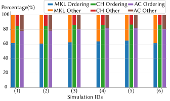
If we then begin to look at the symbolic phase with finer granularity, we see that symbolic computation consists of multiple steps that vary with Cholesky solver implementation. However, all sparse Cholesky solvers require and employ high-quality fill-reducing ordering methods in their symbolic phase. In turn, as we summarize in Figure 9, across all three Cholesky solvers, the fill-reducing ordering is by far the largest bottleneck in each solver’s symbolic analysis steps. Here we see that across benchmark problems, fill-reducing ordering takes an average of , , and of the total symbolic analysis time for MKL, Accelerate, and CHOLMOD respectively. At the same time, we observe that even the most opaque Cholesky solver libraries, which do not provide access to their symbolic analysis otherwise, offer APIs that can be used to replace default fill-reducing ordering implementations with customized methods. Thus, if we can show a significant boost in symbolic fill-reducing ordering, this offers the combined advantages of addressing the symbolic analysis bottleneck while staying modular to take advantage of the current, highly optimized, machine-specific numerical phases in existing high-performance solvers. In the following sections, we will demonstrate that Parth can indeed be cleanly integrated in a plug-and-play fashion into all three solver solutions (and certainly others) for a significant overall performance improvement in linear solve times.
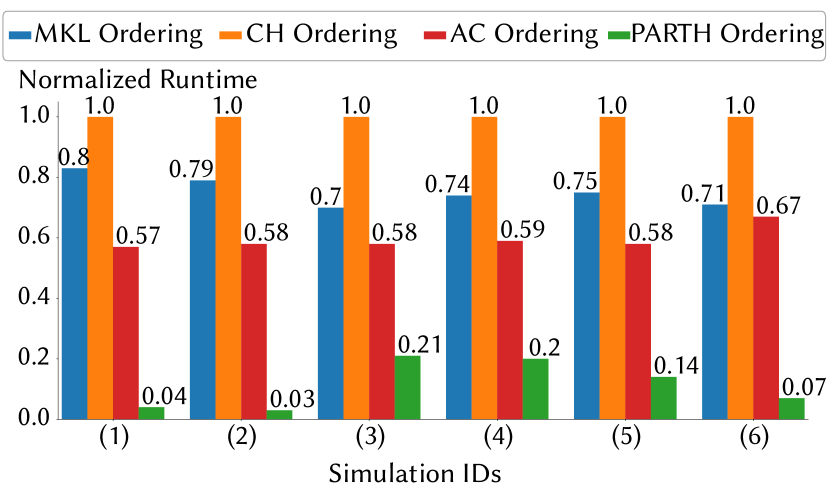
Parth Speedup. the normalized runtime of Parth fill-reducing ordering compared to high-performance Cholesky solvers, namely, MKL, CHOLMOD (CH) and Accelerate (AC). Note that lower is better. The figure is normalized based on the slowest ordering algorithm. Across all 6 simulations, Parth fill-reducing ordering is faster than the fastest tool by 8.04x, 11.66x, 2.29x, 2.75x, 3.70x, and 9.79x speedup from simulation (1) to (6) respectively.
5.4. IPC: Parth Speedup
We first consider here Parth’s speedup in comparison to the fill-reduction timings of all three Cholesky solver libraries across our full benchmark as Parth only accelerates this part of the linear solver pipeline. In Figure 10, we summarize ordering runtimes normalized against the slowest solver. Here we see that Parth outperforms all three Cholesky solvers across all problem sequences in the benchmark, with speedups ranging from X to well over an order of magnitude.
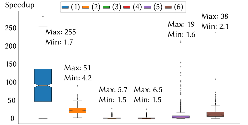
We next push this further and consider an “optimal” competing symbolic analysis which is enabled, without overhead, to pick the fastest ordering among MKL, CHOLMOD and Accelerate (which can otherwise vary per solve for best speeds), for each Newton solve sequence in the benchmark. In Figure 11 we analyze Parth’s speedup against this hypothetical best-speed analysis per Newton-solve sequence. Here we see that, even at the granularity of individual solves, Parth always remains significantly faster than the next best tool with speedups per solve ranging from 1.5x to 255X, across a wide range of solve sequences with both large and small sparsity changes. Note that this is partly due to the Parth compression of graph dual which can be coarsened due to . However, in our Remeshing benchmark, we will see Parth overhead when and Parth does not compress the graph.
5.5. IPC: Parth Ordering Quality
In the above analysis we demonstrate that Parth efficiently computes permutation vectors with significant speedups in comparison to state-of-the-art symbolic methods across diverse sparsity patterns, Hessian sizes, and changing regions of sparsity updates. This demonstrates Parth’s efficient reuse of computation across iterations within Newton solves, per time-step, and across sequential Newton solves, in time-stepped simulation sequences. With timing settled we next analyze here the fill-reduction quality of the orderings computed by Parth, and see that Parth delivers high-quality fill-reduction, comparable to the best sparsity generated among all three compared Cholesky solvers.
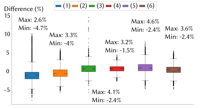
In Figure 12 we compare Parth fill-reduction, with (as in the last section) an imagined, “optimal” competing symbolic analysis method across our benchmark. Specifically, we compare, per linear solve in the benchmark, against the best fill-reducing ordering among MKL, CHOLMOD and Accelerate that generates the sparsest factor. Across all simulation sequences in the benchmark Parth’s permutation quality remains consistent with the best sparse factors computed by the Cholesky solvers’ fill-reduction—largely remaining well within a range, with medians close to zero.
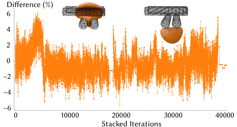
Looking even closer at individual iterations, in Figure 13 we plot the relative sparsity difference in non-zeros between the best-of solution and Parth across the first 40K successive linear solves in the high-contact and compression “Ball Mesh Roller” simulation sequence. Here we see that the total relative sparsity difference comparably remains in a range of .
In summary, we find that across our benchmark, permutation vectors generated by Parth sometimes decrease, and sometimes slightly increase, sparsity (albeit both marginally) over the best provided by top competitor libraries. Recalling that heuristics applied in fill-reducing ordering, e.g. as in METIS (Karypis and Kumar, 1997), lead to similar-scale minor variations in output when executed multiple times on the same problem, we see that Parth then provides comparable quality fill reduction at significant speed-up.
|
|
|
|||||
| (1) Dolphin Funnel | 36154, 35748 | 34625, 35406 | |||||
| (2) Ball mesh roller | 58438, 58212 | 61224, 57925 | |||||
| (3) Mat On Board | 2797, 2788 | 2811, 2817 | |||||
| (4) Rods Twist | 8287, 8210 | 8345, 8267 | |||||
| (5) Squeeze out | 12157,12216 | 12305, 12322 | |||||
| (6) Arma Roller | -, 25950 | 24199, 24655 |
5.6. IPC: Parth Numerical Effect
So far we have demonstrated that across our benchmark Parth generates state-of-the-art quality fill-reduction for its factors with significant runtime speed-ups. A final, and critical, measure of quality for all fill-reduction methods is to sanity check the resulting numerical quality of the symbolic analyses which, for each method, is determined primarily from rounding errors accrued by varying approaches to permutation and parallelization (Anand, 1980). In turn, as discussed above in Section 5.2, these variations lead to changes in the descent directions computed per Newton iteration and so, downstream, the total number of linear solves necessary to complete a simulation. In Table 3, we confirm that Parth-integration preserves the high-quality accuracy, per solve, required for efficient and effective Newton solves. Here, utilizing the saved initial conditions per time-step in our benchmark (see Section 5.2)
We (re-)solve each Newton time-step problem, across each simulation sequence, via the IPC code’s Newton solver, using both default MKL and CHOLMOD solves and our new, Parth-integrated versions. Here we see that Parth-integrated and comparable default solvers converge to the same tolerances, with comparable numbers of iterations for both, demonstrating only minor variations of both slightly larger and smaller iteration counts (With a maximum difference of 5.34% in favour of Parth and 0.14% against Parth). Here, in one notable exception, we observe that MKL is unable to solve a number of iterations in the “Arma Roller” sequence to sufficient accuracy, in turn resulting in non-converging Newton solves and so an incomplete simulation sequence for this portion of the benchmark. This rare but significant failure is not entirely surprising as prior IPC implementations (Li et al., 2023) have avoided MKL Pardiso for this reason. Interestingly, in contrast, we note that Parth-integrated MKL is able to complete more Newton time-step solves for the “Arma Roller” sequence. However, at this time we do not know if this change is due to differences in the quality between a few permutation vectors generated by Parth vs MKL’s custom METIS routines or other code variations in the MKL settings that occur when we pass it custom fill-reducing orderings.
5.7. IPC: Per Sparse Linear Solve Performance
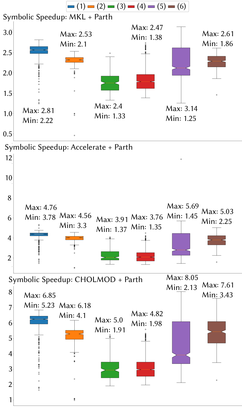
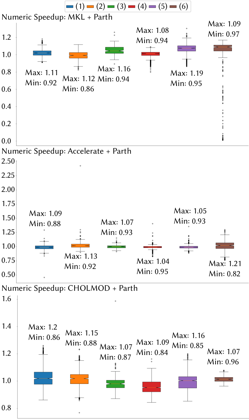
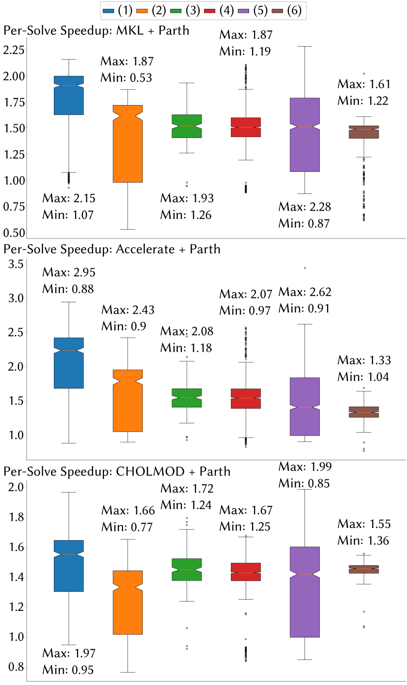
Finally, we consider the performance impact of our three Parth-integrated Cholesky solvers on the symbolic and total costs of linear solves. Following the breakdown in Table 2 we focus on the symbolic analysis phase per solver, In Figure 14, across the benchmark, we see maximum speedups of 8.05x, 5.69x, and 3.14x for CHOLMOD, Accelerate and MKL respectively, with corresponding median speedups of 4.9x, 3.5x, and 2.2x, and minimum speedups of 1.9x, 1.4x, and 1.2x. As covered in Sections 5.5 and 5.6, with this speedup, Parth still maintains state-of-the-art fill-in and comparable numerical quality to CHOLMOD and Accelerate (recalling that we observe MKL has occasional but catastrophic failures in accuracy). This suggests that Parth-integrated solves should provide symbolic speedup while leaving the already significantly optimized performance of numerical computation steps (including the Cholesky factorization and sparse triangular forward/backward solves) unharmed. We see this confirmed for all three solvers in Figure 15, where we confirm integration of Parth brings the above speedup without additional overhead elsewhere in the already optimized numerical computations of the Cholesky solver packages.
In Figure 16 we see that by just direct integration of the Parth module into Cholesky solver packages, we obtain speedups on full Cholesky solve costs of up to 2.95X, 2.28X and 1.97X (1.5X, 1.54X, and 1.43X median) for Accelerate, MKL and CHOLMOD respectively. In line with our earlier analysis, we also confirm that Parth consistently extracts the greatest performance speedups as it is integrated with successively more optimized and more performant Cholesky solvers taking advantage of hardware – here in Accelerate and then following with MKL. In Table 4 we correspondingly report the total Cholesky-solver runtime costs across all linear solves for each simulation sequence in the benchmark, and again observe consistent breakdowns.
There are two important takeaways from Table 4. First, the Cholesky solve baselines currently used by practitioners are not the fastest possible, leading to confusion and suboptimal choices when integrating fast direct and approximate solvers. For example, IPC involves multiple steps, and to achieve fast end-to-end acceleration, all these steps must be optimized (Huang et al., 2024). However, selecting the best linear solver requires balancing accuracy and speedup. For instance, Huang et al. (2024) presents a sophisticated computational pipeline for IPC that leads to impressive end-to-end speedup, but their linear solve baseline is not well optimized. In their paper, they provide a detailed evaluation of their linear solvers, including speedups and failure cases. The reported 4x speedup over CHOLMOD for their PCG linear solve comes with the drawback of potential failures in some benchmarks (as reported in (Huang et al., 2024)). However, by looking at Table4, we observe that switching from CHOLMOD to Apple Accelerate on an M2 processor, combined with integrating Parth, can deliver up to 6x speedup over CHOLMOD, with an average speedup of 4.07x. This means a practitioner could opt to use the CCD strategy from (Huang et al., 2024) along with a Parth-integrated Apple Accelerate, benefiting from both the performance improvements in CCD and the numerical stability of a Cholesky solve. This highlights one of the key contributions of our work: providing a crucial comparison between different Cholesky solvers.
The second important takeaway is the runtime savings achieved by integrating Parth. For example, consider using CHOLMOD for the “Arma Roller” simulation due to its numerical stability on an Intel processor. While the solve speedup is 1.45x, the 45% reduction in runtime translates to a savings of 9.75 hours. Given the minimal overhead required to integrate Parth (3 lines of code) and its consistent numerical stability, many practitioners can easily gain these performance benefits without needing to refactor an entire computational pipeline, which is often not a straightforward task.
| Parth + Tool | Step | Dolphin Funnel | Ball Mesh Roller | Mat On Board | Rods Twist | Squeeze out | Arma Roller |
| Symbolic time(s) | 3261 1424 | 2623 1134 | 1551 914 | 5363 2481 | 9098 4425 | 35357 15714 | |
| MKL | Numeric time(s) | 932 923 | 1085 1075 | 485 457 | 2800 2751 | 2543 2397 | 30703 32335 |
| Symbolic time(s) | 1773 490 | 1465 369 | 985 483 | 5363 2481 | 5540 2119 | 25331 6913 | |
| Accelerate | Numeric time(s) | 706 709 | 861 861 | 412 412 | 2578 2602 | 2231 2251 | 51871 51098 |
| Symbolic time(s) | 2857 597 | 2353 453 | 1600 558 | 8552 2764 | 9012 2422 | 35021 6696 | |
| CHOLMOD | Numeric time(s) | 4200 4106 | 4511 4432 | 1663 1727 | 9098 9385 | 9483 9499 | 58282 57492 |
5.8. Remeshing: Benchmark
In this section we next evaluate how Parth performs in remeshing applications where sparsity patterns change due to localized updates in mesh geometry and topology which result in both adding and deleting of the nodes in G and added and removed edges. Here we test with a remeshing pipeline in which we select remeshing patch regions on triangle meshes, remesh with Botsch and Kobbelt (2004) to alter patch structure, and then apply global discrete Laplacian operator (Jacobson et al., 2024). For comprehensive analysis, remeshing operations are chosen to cover patches with a range of sizes comprising 1%, 5%, 10%, 20% of the faces. Each patch is created around a randomly selected face ID. Here, per each mesh, the same face ID is used for comparison between different linear solvers. As a result, comparisons across linear solvers for a specific mesh and patch is consistent with identical computation. For each patch size, fifty such samples are chosen, covering different areas of a surface mesh, forming 200 sparse linear solves per mesh. After applying each patch remeshing, we reset the mesh and select another patch to measure Parth’s reuse capability for each patch size. This testing is applied across all the meshes in the Stein (2024) repository with the exclusion of the overly simple Cube mesh.
In addition to testing an application with changing matrix size, this benchmark additionally allows evaluation of Parth’s performance on triangular meshes, and on linear solves with a problem dimension of (recalling for IPC, it is 3). As a result, in this evaluation, Parth directly employs the graph dual of the input matrix instead of the coarsened version where the graph nodes associated with a single DOF are combined. As a result, this benchmark does not require application of Parth’s compression.
5.9. Remeshing: Bottleneck Analysis
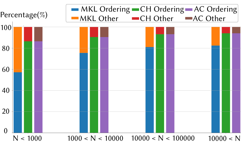
Figure 17 provides an analysis of the bottleneck of the symbolic stage. Here, we divide the meshes into separate groups based on their number of DOFs to show the effect of mesh sizes on the symbolic analysis stage. As we increase mesh size, and consequently increase the size of the graph dual of the Laplacian operator, the fill-reducing ordering performance overhead becomes more prominent. For example, for small meshes, fill-reducing ordering is 57% of the symbolic analyzing, and for Large meshes, this overhead increases to 82% for the MKL solver. As a result, for large-scale problems, optimizing symbolic analysis is clearly important for the Cholesky solve pipeline. Note that these results are consistent with our analysis of the IPC benchmark.
5.10. Remeshing: Total Linear Solve Performance
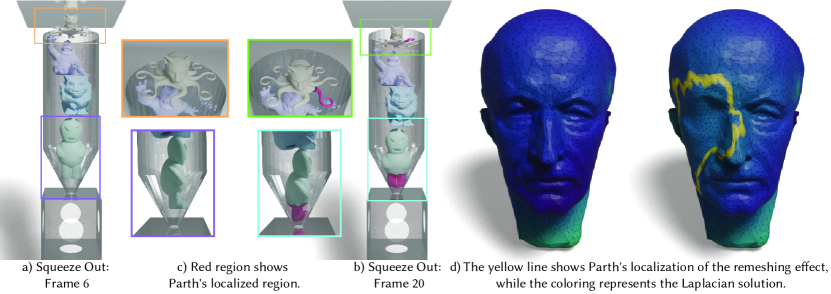
Here we discuss only the symbolic analysis and total per-solve linear solve performance of the remeshing benchmark. However, consistent with our IPC benchmark analysis, we also provide our numerical performance analysis of the remeshing benchmark in Appendix G. For this set of analyses, we divide the performance data into five categories. The first category is the initialization step, while the next four categories reflect performance with respect to patch size. This categorization allows us to offer further insight into Parth’s initialization cost without the compression phase, making the overhead of building the HGD data structure more visible. Furthermore, as shown in the teaser, a 2% selection of the surface mesh is not considered small. By increasing these patch sizes to 20%, we aim to provide insight into more challenging situations where the changes are more drastic, demonstrating Parth’s performance in terms of both reuse capability and fill-reducing quality.
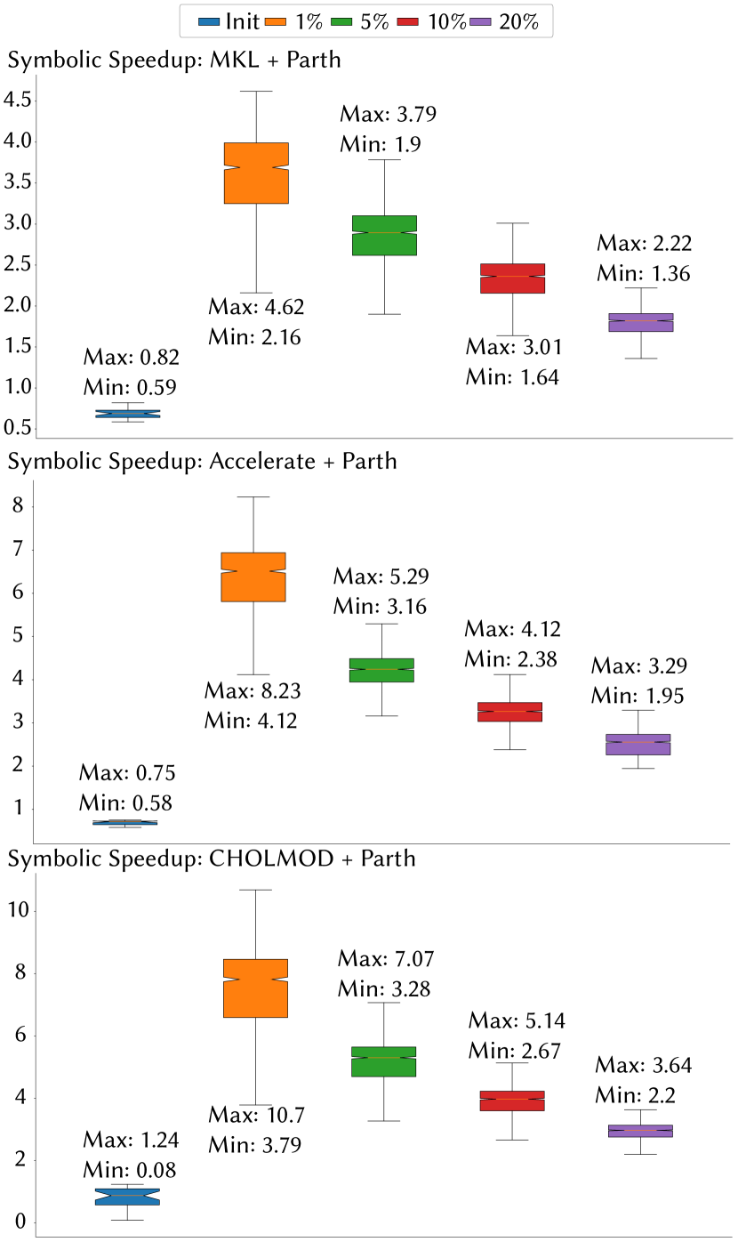
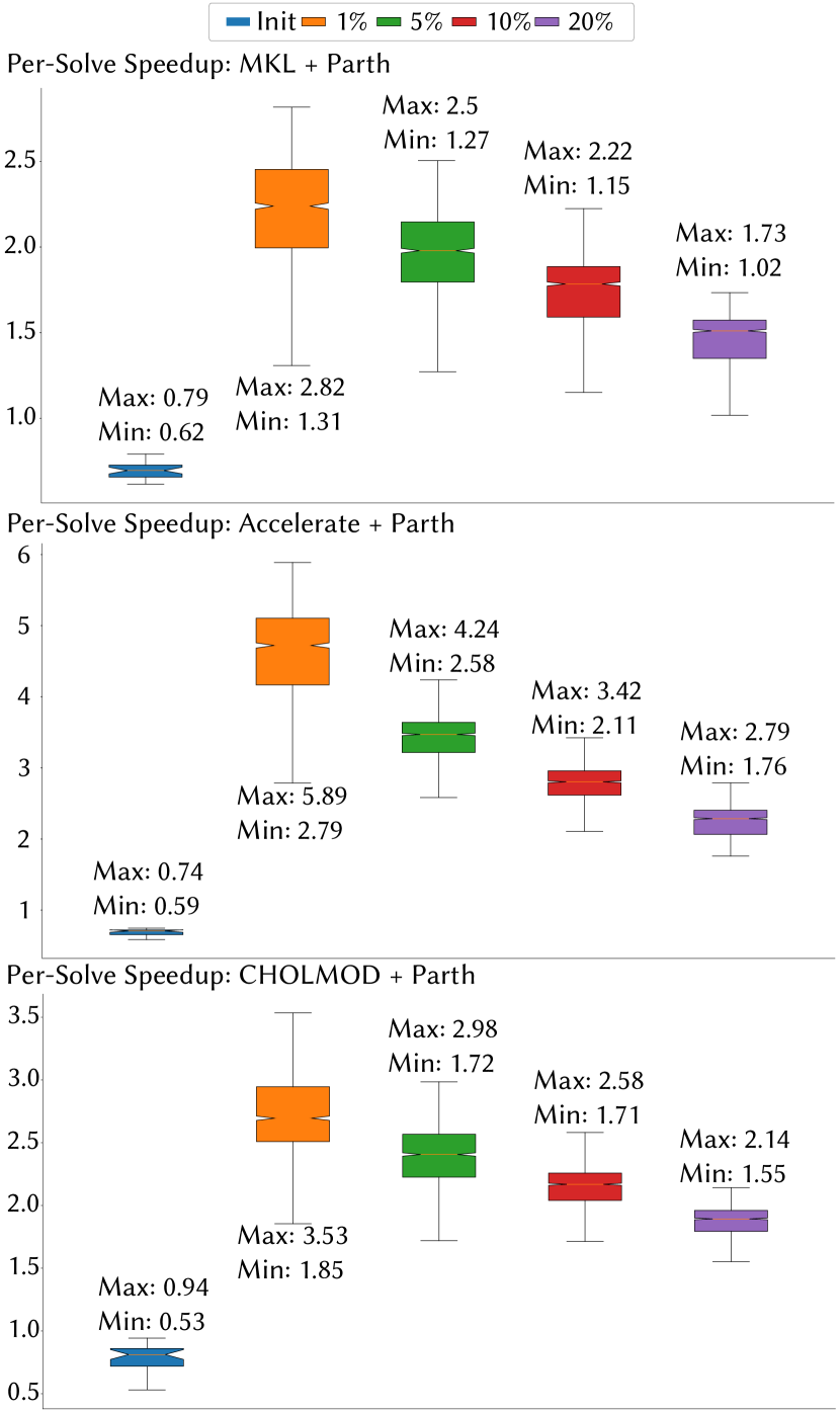
Figure 18 shows Parth’s effect on the symbolic analysis. As expected, since for this computational pipeline, Parth reduces performance in the initialization step. However, since the HGD computation is also reused in the fill-reducing ordering computation, the average performance speed is 70% of the baseline fill-reducing routine. After the initialization step, Parth consistently provides speedup. For example, in CHOLMOD with patch sizes of 1%, Parth achieves an order-of-magnitude speedup. It is important to note that as the size of the patches on the mesh increases, Parth’s performance decreases due to less temporal coherence and fewer opportunities for reuse, i.e., the changes become less gradual. In patch sizes of 20%, for instance, we observe up to a 3.36x speedup, which is smaller than the order-of-magnitude speedup achieved with patch sizes of 1% of the surface faces in symbolic analysis.
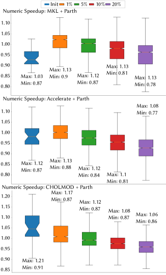
The performance benefits in symbolic analysis lead to an overall improvement in total Cholesky solve time, as shown in Figure 18. As expected, this performance boost mirrors the trends seen in symbolic analysis, resulting in up to a 5.89x, 3.55x, and 2.82x speedup compared to Accelerate, CHOLMOD, and MKL, respectively.
6. Limitations and Future Work
Currently, Parth is designed to provide performance benefits by reusing symbolic analysis computations. However, when the computational bottleneck is not symbolic analysis, and specifically not fill-reducing ordering, Parth’s improvement is not applicable. We plan to address this limitation by adding comparable and complementary adaptive numerical acceleration techniques to Cholesky solves.
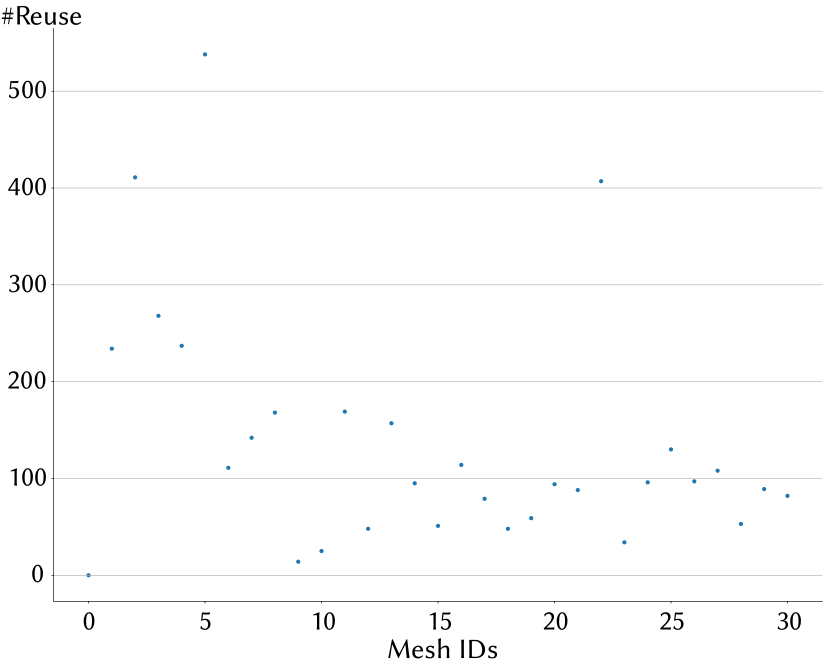
Another important limitation for future investigation is how long Parth can preserve high-quality fill-reducing ordering performance, as finding high-quality fill-reducing ordering generally requires global information. To assess Parth’s limitations, we apply remeshing to 1,000 patches, each comprising 1% of mesh faces, on the triangular meshes evaluated in our remeshing benchmark. Each of these 1,000 patches is selected around face IDs that were not chosen in the previous patch, and the selection is made from a uniform distribution. This randomness allows for the evaluation of different scenarios while modifying the triangle meshes. Here, we evaluate how many applications of these 1% patch remeshings can be applied before the performance of numerical computation drops below 85% of the baseline. This, in turn, indicates how many times Parth can generally provide high-quality reuse without recomputing an entire fill-reducing ordering. Note that for this test, the aggressive reuse algorithm (Appendix E) is activated to ensure that Parth does not recompute the full fill-reducing ordering when a patch on the root separator changes.
In Figure 20, we see the results of this test, with the x-axis showing mesh IDs from (Stein, 2024), sorted by the number of DOF, and the y-axis indicating the number of reuses. As shown, for some meshes, Parth can maintain high-quality fill-reducing ordering even after 500 applied patches. On average, performance drops below 85% after 70 remeshings of distinct patches, which approximately result in 70% changes to the mesh. However, this generally depends on the shape of the mesh and the degree of deformation caused by the remesher. On average, after approximately 70% changes to the triangle meshes, Parth needs to be reset to obtain new fill-reducing ordering information, as the underlying geometry has changed significantly.
7. Conclusion and Discussion
In summary, our evaluation confirms that the Parth module provides successful, simple and direct integration into all three state-of-the-art Cholesky solver libraries. Parth generates for each, across widely ranging and challenging linear systems in our benchmark, comparable, high-quality fill-in reduction – critical for efficient sparse linear solves. At the same time Parth delivers an up to 255x speedup for fill-reducing ordering computation, while preserving the numerical stability and performance in the resulting downstream Cholesky factorization and subsequent solve processes of all three solver libraries, resulting in an up to 6x speedup in overall direct solve times – Outperforming the best speedups obtained by recent architecture-customized Cholesky solver updates (Inc., 2023). As direct solvers are a core and sometimes unavoidable bottleneck in applications with dynamically changing sparsity, this represents a significant improvement obtained by a simple module addition, at just the API level per-solver. We expect this enhancement will likewise, as proofed out here across solvers, be equally applicable to other and future-developed improved Cholesky solver packages.
We have presented a new comprehensive benchmark for fair side-by-side evaluation of Cholesky solvers across sequential, highly challenging practical linear solve systems, with dynamically changing and coherent sparsity transitions. We have then presented a new and extensive evaluation of state-of-the-art Cholesky solvers on this benchmark. Both of these first two contributions have directly led to the insights enabling the new Parth module’s perfromance boost and we expect that this benchmarking can and will lead to more comparable improvements in this challenging and important area critical across domains in computer graphics ranging from physics simulation to deformation processing and adaptive remeshing to name just a few.
At the same time we have extensively evaluated our new Parth module to demonstrate its advantages in challenging applications with rapid sparsity change – contacting elastodynamics simulation and remeshing. Looking ahead, we observe that Parth is a quite general solution and so we expect its flexibility and efficiency should be a widely applicable solution for improving the fill-reducing ordering runtime for high-performance direct solvers in diverse applications with changing sparsity patterns. Parth’s flexibility is likewise evidenced in that it requires no-per application tuned parameters, and its underlying algorithm does not rely on the type of algorithm applied in creating and solving the sequential linear systems treated and so should be generally applicable. Likewise, although we focus entirely here on its performance benefits for direct solvers, we look ahead to interesting investigations in it potential application to preconditioning methods, including both linear and nonlinear methods (Li et al., 2019). Finally we observe that with our long-term goal of easy plug-and-play generality we have likely left many domain specific improvements possible for even further speedups.
References
- (1)
- IPC (2020) 2020. IPC. https://github.com/ipc/ipc-sim GitHub repository.
- Amdahl (1967) Gene M Amdahl. 1967. Validity of the single processor approach to achieving large scale computing capabilities. In Proceedings of the April 18-20, 1967, spring joint computer conference. 483–485.
- Amestoy et al. (2004) Patrick R Amestoy, Timothy A Davis, and Iain S Duff. 2004. Algorithm 837: AMD, an approximate minimum degree ordering algorithm. ACM Transactions on Mathematical Software (TOMS) 30, 3 (2004), 381–388.
- Anand (1980) Indu Mati Anand. 1980. Numerical stability of nested dissection orderings. Math. Comp. 35, 152 (1980), 1235–1249.
- Bischoff et al. (2002) Botsch Steinberg Bischoff, M Botsch, S Steinberg, S Bischoff, L Kobbelt, and Rwth Aachen. 2002. OpenMesh–a generic and efficient polygon mesh data structure. In In openSG symposium, Vol. 18.
- Botsch and Kobbelt (2004) Mario Botsch and Leif Kobbelt. 2004. A remeshing approach to multiresolution modeling. In Proceedings of the 2004 Eurographics/ACM SIGGRAPH symposium on Geometry processing. 185–192.
- Chen et al. (2008) Yanqing Chen, Timothy A Davis, William W Hager, and Sivasankaran Rajamanickam. 2008. Algorithm 887: CHOLMOD, supernodal sparse Cholesky factorization and update/downdate. ACM Transactions on Mathematical Software (TOMS) 35, 3 (2008), 1–14.
- Cheshmi et al. (2017) Kazem Cheshmi, Shoaib Kamil, Michelle Mills Strout, and Maryam Mehri Dehnavi. 2017. Sympiler: transforming sparse matrix codes by decoupling symbolic analysis. In Proceedings of the International Conference for High Performance Computing, Networking, Storage and Analysis. 1–13.
- Cheshmi et al. (2018a) Kazem Cheshmi, Shoaib Kamil, Michelle Mills Strout, and Maryam Mehri Dehnavi. 2018a. ParSy: inspection and transformation of sparse matrix computations for parallelism. In SC18: International Conference for High Performance Computing, Networking, Storage and Analysis. IEEE, 779–793.
- Cheshmi et al. (2018b) Kazem Cheshmi, Shoaib Kamil, Michelle Mills Strout, and Maryam Mehri Dehnavi. 2018b. ParSy: Inspection and transformation of sparse matrix computations for parallelism. In SC18: International Conference for High Performance Computing, Networking, Storage and Analysis. IEEE, 779–793.
- Cheshmi et al. (2020) Kazem Cheshmi, Danny M Kaufman, Shoaib Kamil, and Maryam Mehri Dehnavi. 2020. NASOQ: numerically accurate sparsity-oriented QP solver. ACM Transactions on Graphics (TOG) 39, 4 (2020), 96–1.
- Cheshmi et al. (2023) Kazem Cheshmi, Michelle Strout, and Maryam Mehri Dehnavi. 2023. Runtime composition of iterations for fusing loop-carried sparse dependence. In Proceedings of the International Conference for High Performance Computing, Networking, Storage and Analysis. 1–15.
- Davis and Hager (2005) Timothy A Davis and William W Hager. 2005. Row modifications of a sparse Cholesky factorization. SIAM J. Matrix Anal. Appl. 26, 3 (2005), 621–639.
- Davis et al. (2016) Timothy A Davis, Sivasankaran Rajamanickam, and Wissam M Sid-Lakhdar. 2016. A survey of direct methods for sparse linear systems. Acta Numerica 25 (2016), 383–566.
- Dongarra et al. (1990) Jack J Dongarra, Jeremy Du Croz, Sven Hammarling, and Iain S Duff. 1990. A set of level 3 basic linear algebra subprograms. ACM Transactions on Mathematical Software (TOMS) 16, 1 (1990), 1–17.
- Herholz and Alexa (2018) Philipp Herholz and Marc Alexa. 2018. Factor once: reusing cholesky factorizations on sub-meshes. ACM Transactions on Graphics (TOG) 37, 6 (2018), 1–9.
- Herholz and Sorkine-Hornung (2020) Philipp Herholz and Olga Sorkine-Hornung. 2020. Sparse cholesky updates for interactive mesh parameterization. ACM Transactions on Graphics (TOG) 39, 6 (2020), 1–14.
- Huang et al. (2024) Kemeng Huang, Floyd M Chitalu, Huancheng Lin, and Taku Komura. 2024. GIPC: Fast and stable Gauss-Newton optimization of IPC barrier energy. ACM Transactions on Graphics 43, 2 (2024), 1–18.
- Inc. (2023) Apple Inc. 2023. Accelerate Framework. Available at https://developer.apple.com/documentation/accelerate.
- Jacobson et al. (2024) Alec Jacobson, Daniele Panozzo, et al. 2024. Libigl Tutorial - Laplace Equation. https://libigl.github.io/tutorial/#laplace-equation. Accessed: 2024-10-18.
- Jacobson et al. (2013) Alec Jacobson, Daniele Panozzo, C Schüller, Olga Diamanti, Qingnan Zhou, N Pietroni, et al. 2013. libigl: A simple C++ geometry processing library. Google Scholar (2013).
- Karypis and Kumar (1997) George Karypis and Vipin Kumar. 1997. METIS: A software package for partitioning unstructured graphs, partitioning meshes, and computing fill-reducing orderings of sparse matrices. (1997).
- Khaira et al. (1992) Manpreet S Khaira, Gary L Miller, and Thomas J Sheffler. 1992. Nested Dissection: A survey and comparison of various nested dissection algorithms. Carnegie-Mellon University. Department of Computer Science.
- Li et al. (2021) Jing Li, Tiantian Liu, Ladislav Kavan, and Baoquan Chen. 2021. Interactive cutting and tearing in projective dynamics with progressive cholesky updates. ACM Transactions on Graphics (TOG) 40, 6 (2021), 1–12.
- Li et al. (2020) Minchen Li, Zachary Ferguson, Teseo Schneider, Timothy R Langlois, Denis Zorin, Daniele Panozzo, Chenfanfu Jiang, and Danny M Kaufman. 2020. Incremental potential contact: intersection-and inversion-free, large-deformation dynamics. ACM Trans. Graph. 39, 4 (2020), 49.
- Li et al. (2023) Minchen Li, Zachary Ferguson, Teseo Schneider, Timothy R Langlois, Denis Zorin, Daniele Panozzo, Chenfanfu Jiang, and Danny M Kaufman. 2023. Private Correspondence with IPC Authors. Personal Communication.
- Li et al. (2019) Minchen Li, Ming Gao, Timothy Langlois, Chenfanfu Jiang, and Danny M Kaufman. 2019. Decomposed optimization time integrator for large-step elastodynamics. ACM Transactions on Graphics (TOG) 38, 4 (2019), 1–10.
- Liu (1990) Joseph WH Liu. 1990. The role of elimination trees in sparse factorization. SIAM journal on matrix analysis and applications 11, 1 (1990), 134–172.
- Liu et al. (2021) Yang Liu, Pieter Ghysels, Lisa Claus, and Xiaoye Sherry Li. 2021. Sparse approximate multifrontal factorization with butterfly compression for high-frequency wave equations. SIAM Journal on Scientific Computing 43, 5 (2021), S367–S391.
- Pellegrini (2009) François Pellegrini. 2009. Distillating knowledge about Scotch. In Dagstuhl Seminar Proceedings. Schloss Dagstuhl-Leibniz-Zentrum für Informatik.
- Pfaff et al. (2014) Tobias Pfaff, Rahul Narain, Juan Miguel De Joya, and James F O’Brien. 2014. Adaptive tearing and cracking of thin sheets. ACM Transactions on Graphics (TOG) 33, 4 (2014), 1–9.
- Rennich et al. (2016) Steven C Rennich, Darko Stosic, and Timothy A Davis. 2016. Accelerating sparse Cholesky factorization on GPUs. Parallel Comput. 59 (2016), 140–150.
- Schenk et al. (2001) Olaf Schenk, Klaus Gärtner, Wolfgang Fichtner, and Andreas Stricker. 2001. PARDISO: a high-performance serial and parallel sparse linear solver in semiconductor device simulation. Future Generation Computer Systems 18, 1 (2001), 69–78.
- Schmidt et al. (2023) Patrick Schmidt, Dörte Pieper, and Leif Kobbelt. 2023. Surface maps via adaptive triangulations. In Computer Graphics Forum, Vol. 42. Wiley Online Library, 103–117.
- Sellán et al. (2020) Silvia Sellán, Jacob Kesten, Ang Yan Sheng, and Alec Jacobson. 2020. Opening and closing surfaces. ACM Transactions on Graphics (TOG) 39, 6 (2020), 1–13.
- Stein (2024) Oded Stein. 2024. odedstein-meshes: A Computer Graphics Example Mesh Repository. (2024).
- Yannakakis (1981) Mihalis Yannakakis. 1981. Computing the minimum fill-in is NP-complete. SIAM Journal on Algebraic Discrete Methods 2, 1 (1981), 77–79.
Appendix A HGD Computation Reused in Fill-reducing Ordering
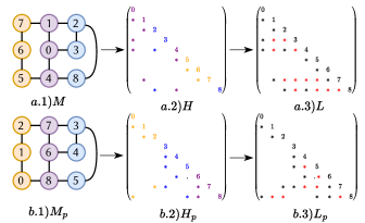
To further illustrate how the information in contributes to fill-reducing ordering computation, refer to Figure 21. In this figure, the separator set, colored in purple, is used in reducing fill-ins. The procedure effectively renumbers the nodes in the such that the computation of the separator set occurs at the end of the factor computation. When comparing Figures 21(a.1) and 21(b.1), it becomes apparent that the graph undergoes renumbering, positioning the separator set numbers after the orange and blue colored left and right sub-meshes, respectively. A comparison of the matrix in Figure 21(a.2) with in Figure 21(b.2) shows an identical count of non-zero entries; however, their sparsity patterns differ due to the renumbering. Factoring both and shows that the factor possesses fewer fill-ins than , thus demonstrating fill-reduction achieved by the permutation.
Appendix B Node Change Synchronizer
By removing or adding a set of nodes from a graph , a new graph is created. By adding and removing nodes, the indices of the nodes in change. For example, Figure 22 illustrates how removing a node and adding a new one can alter the labeling of the node in a graph. The objective of this heuristic is to synchronize with the to represent the latest node structure. Furthermore, it provides the necessary information for the Assembler module to update the permutation vector accordingly.
The Synchronizer uses the map array to detect the added and removed nodes in the graph. To formally define the map, is a function , where represents all the node indices in , denoted as , and similarly, . Any node that is in but not in the range of (for example, node 0 is not in the range of in Figure 22(a)) is considered a deleted node. Additionally, any node for which is an added node. It is natural to assume that if , then , which implies that no two nodes in can be mapped to a single node in . Based on our experience, this map is a common structure in remesher libraries, and we successfully extract this information from the subroutines used in remeshers such as those in (Schmidt et al., 2023; Pfaff et al., 2014; Bischoff et al., 2002; Botsch and Kobbelt, 2004). The loop subdivision of IGL (Jacobson et al., 2013) also provides this information as output. Algorithm 4 describe the synchronization process, which is performed in 3 steps as follows:
Step 1: Deleting the removed nodes from : In the first step of this heuristic, Parth deletes the removed nodes from . This process also involves updating the local accordingly (see Section 4.3 and Lines 4-8 in Algorithm 4). For example, in Figure 22(a), the removed nodes are identified using the map since they are not present in the range of the map. Then, in Figure 22(b), this node is deleted from .
Step 2: Updating the indices: By adding and deleting DOFs from a mesh and renaming the DOFs based on that process, the corresponding naming of the nodes in the graph also changes. As a result, it is crucial to update the indices of the nodes to maintain consistency. Using the , Parth updates the indices (Line 9). For example, in Figure 22(b), since the new name for node 8 in is 0, the indices of nodes in the sub-graph represented by are updated from to . In practice, Steps 1 and 2 are applied simultaneously for computational reuse.
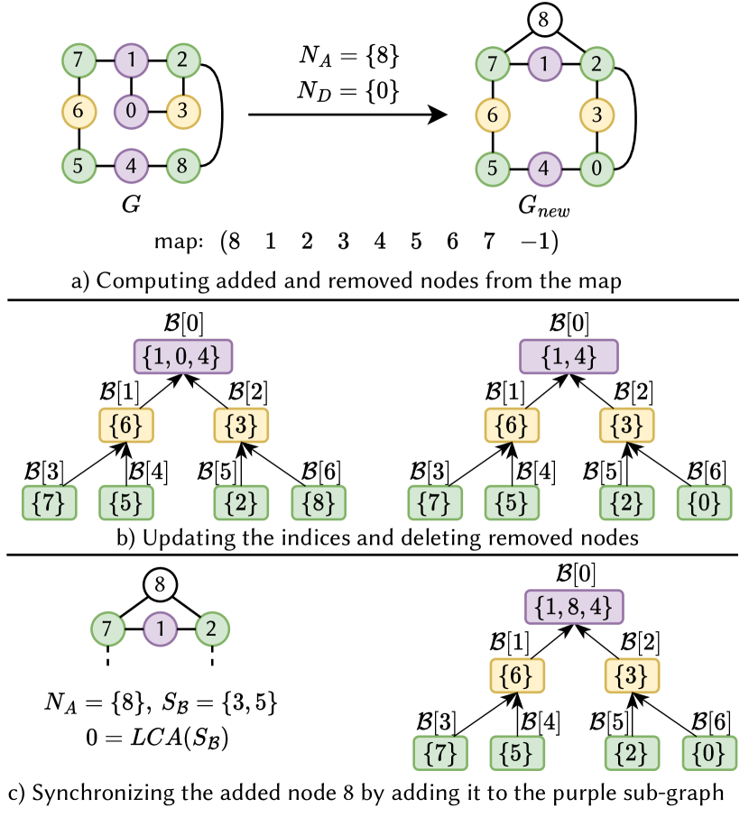
Step 3: Assign a sub-graph to each added node: After updating the indices and deleting the nodes, the Synchronizer assigns the added nodes to (Lines 11-34). Parth uses a heuristic that assigns the nodes to each sub-graph based on their neighbors. For each added node, he first computes all the sub-graphs that are adjacent to it. If there is only a single sub-graph, then that node is assigned to that sub-graph. If it is adjacent to more than one sub-graph, the lowest common ancestor in is selected as the sub-graph to which it will be assigned. As an example, see Figure 22(c). By doing so, we maintain the separator relation across each sub-graph. Finally, this process repeats in a greedy manner to assign all the nodes to sub-graphs. If a completely separated graph is added, Parth simply assigns that separated graph to a leaf in .
Appendix C Synchronizer: Dirty Sub-Graph Detection
The objective of the algorithm 5 is to first categorize the edges into three groups. (I) The edges that show a change in connectivity within a sub-graph. (II) The edges that connect a separator set to its left and right sub-graphs. (III) Finally, the edges violate a separator condition by connecting two sub-graphs that are otherwise completely separated from each other. Lines (3–5) detect the first group by checking whether the two ends of the edge are within the same sub-graph, i.e., . Line 7 distinguishes between groups (II) and (III). If this condition is true, it means that the edge is between a separator and its corresponding left and right sub-graphs. Otherwise, it violates a separator. To find this separator, we simply need to find the Lowest Common Ancestor (LCA) of the two sub-graphs, a and b, by traversing the (line 8).
Appendix D Synchronizer: Mark And Decompose Sub-Graphs
Algorithm 6 uses the sets and to assign values to the cache . This array is then used as an indicator of sub-graphs that need an updated local permutation vector (see Section 4.3). The entries of are computed in two steps. First, fine-grain sub-graphs indicated by are marked as not cached in . This means that the fill-reducing ordering information for these sub-graphs is not valid and needs to be recomputed by Assembler. To handle changes in coarse-grain sub-graphs, the HGD algorithm is used to re-decompose them, creating a set of valid separators. Lines 5-8 first extract the coarse-grain sub-graph, then apply the HGD algorithm for re-decomposition. Note that the input to HGD is defined so that the sub-tree in representing the coarse-grain sub-graph is replaced with a new sub-tree containing the same number of sub-graphs (same sub-tree structure). After computing a valid set of sub-graphs, each of the sub-graphs is marked as not cached in (line 10) so that Assembler can recompute the fill-reducing ordering for each of them.
Appendix E Synchronizer: Aggressive Reuse
One of the problems with the Parth pipeline is the strict requirement that even for a single violation between two sub-graphs, with the root of as their lowest common ancestor, the reuse is zero. Although this effect sometimes occurs in our IPC benchmark, it does not result in significant performance loss. However, since we provide whisker plots of speedups to show the wide range of possible outcomes with various meshes and configurations of local changes, we also need to address this problem.
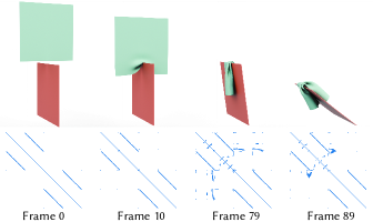
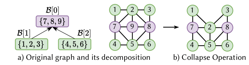
Based on the IPC benchmark, we observe that zero reuse can happen when two objects collide. In these scenarios, the root in is an empty set when the objects are not colliding (see Frame 0 in Figure 23). At the moment of collision, reuse is zero because the empty root is no longer a separator. The point of contact then becomes the separator (Frame 7). If the contact area includes a small number of DOFs, fluctuations in the contact area result in zero reuse. However, when the contact area increases, this problem is no longer significant, as the separator is no longer solely the point of contact. This can also occur in the remeshing benchmark, for example, when a DOF corresponding to a separator node in the graph collapses into its left or right sub-meshes. This results in all the edges connected to that separator violating the separator sub-graph condition (see Figure 24 for an example). To alleviate this problem, Parth uses Algorithm 7 to provide reuse even in these scenarios.
Algorithm 7 performs the reallocation in two steps. First, it counts the number of occurrences of each node in , which are the problematic edges (Step 1, Lines 1-5). In Step 2, similar to how the Synchronizer module detects and resolves changes in the graph, it finds the edges that have an LCA less than a user-defined level (). In other words, the user can define when not to re-decompose a coarse-grained sub-graph using this variable. By detecting the separator set that has a problem with a specific edge <a,b>using the LCA function, the node with higher occurrence is moved to that specific separator sub-graph. Note that this heuristic is a greedy approach to reduce the number of nodes reallocated to the separator sub-graph, as we do not want to significantly increase the separator sizes. Also, note that we omit implementation details here. For example, Parth checks whether a node has already been reallocated or not. However, these details can be found in the open-source code.
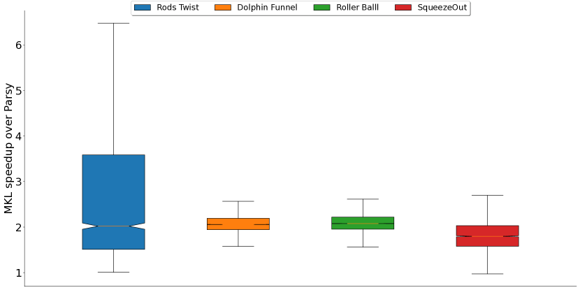
Appendix F Parsy and Eigen Performance
Figure 25 shows how the numerical performance of MKL is now faster than Parsy by an average of 2.7x, 2.08x, 2.09x, 1.84x on Rode Twist, Dolphin Funnel, Roller Ball and Squeeze Out simulation on IPC (Li et al., 2020) benchmark. This evaluation shows that not only MKL cached up to the Sympiler library which uses both Sympiler (Cheshmi et al., 2017) and Parsy (Cheshmi et al., 2018a) contributions, but it also significantly outperforming them due to its constant development with state-of-the-art hardwares. Due to this reason, we decide to develop Parth so it can be integrated into these solver and provide performance benefits on top of the performance benefits gained by these high-performance linear solver.
Appendix G Remeshing: Fill-reducing Quality Analysis
Figure 26 shows Parth’s initialization performance is on par with state-of-the-art fill-reducing ordering algorithms. For 1% changes, Parth outperforms Accelerate and MKL in median speedup. As expected, performance decreases with larger patches due to the global nature of fill-reducing ordering, but even at 20% changes, the median speedup remains around 0.95x. Given the significant symbolic-stage gains, this minor trade-off is acceptable, as shown in Section 5.