Synthetic Data for Portfolios:
A Throw of the Dice Will Never Abolish Chance

Abstract

Simulation methods have always been instrumental in finance, and data-driven methods with minimal model specification—commonly referred to as generative models—have attracted increasing attention, especially after the success of deep learning in a broad range of fields. However, the adoption of these models in financial applications has not kept pace with the growing interest, probably due to the unique complexities and challenges of financial markets. This paper aims to contribute to a deeper understanding of the limitations of generative models, particularly in portfolio and risk management. To this end, we begin by presenting theoretical results on the importance of initial sample size, and point out the potential pitfalls of generating far more data than originally available. We then highlight the inseparable nature of model development and the desired use case by touching on a paradox: generic generative models inherently care less about what is important for constructing portfolios (in particular the long-short ones). Based on these findings, we propose a pipeline for the generation of multivariate returns that meets conventional evaluation standards on a large universe of US equities while being compliant with stylized facts observed in asset returns and turning around the pitfalls we previously identified. Moreover, we insist on the need for more delicate evaluation methods, and suggest, through an example of mean-reversion strategies, a method designed to identify poor models for a given application based on regurgitative training, i.e. retraining the model using the data it has itself generated, which is commonly referred to in statistics as identifiability.

Keywords: generative models, synthetic data, machine learning, generative adversarial networks, high-dimensional returns, principal component analysis, portfolio construction

1 Introduction

In 1887, the French poet Stéphane Mallarmé composed “Un coup de dés jamais n’abolira le hasard” (in English A Throw of the Dice will Never Abolish Chance), which was a first step in the direction of concrete poetry. In a context of the flourishing scientific developments in Europe, especially in probability and statistics (think about Adolphe Quetelet and Bernoulli’s and Poisson’s work on the “loi des grands nombres”, the law of large numbers), the message of the poem was as simple as its title: in the context of randomness, drawing one realization does not cancel the reality of the underlying stochastic phenomenon. This paper is about that: in the highly non-stationary and high-dimensional realm of returns of financial instruments, drawing synthetic data made of the informational content of a small sample is not abolishing the depth of this initial randomness.

The practice of drawing samples from a model to address specific financial tasks dates back to at least the 1960s, when [Hertz, 1964] proposed using simulations for investment risk analysis. The potential of this approach was quickly realized for the valuation of options, with one of the earliest applications appearing in [Boyle, 1977]. The adoption of such techniques, along with the effort to develop more realistic models, has grown significantly with the increasing complexity of derivatives pricing (e.g., [Broadie and Glasserman, 1996] and [Carriere, 1996]), the need for stress-testing and accurate risk estimation (e.g., Value-at-Risk) for large portfolios of non-linear instruments (e.g., [Berkowitz, 1999] and [Jamshidian and Zhu, 1996]), and the optimization of portfolios with sensitivity to extreme losses [Rockafellar and Uryasev, 2000], among many other applications across various areas in finance.

The conventional approach, known as Monte Carlo methods (see [Glasserman, 2004] and [Jäckel, 2002]), involves random sampling from a parametric model specified by the user to ensure that it accurately represents the process, distribution, or environment being modeled. The parameters of the specified model are typically calibrated using the available historical data. Despite the interpretability provided by the parametric nature of the model, a major limitation of this approach is its inherent dependence on the initial assumptions about the model design, which might not accurately reflect the underlying reality. Another drawback is its questionable scalability as the complexity of the system increases, requiring the user to have an extremely deep understanding of the environment—a task that can be practically impossible in some cases.

Therefore, machine learning methods that make minimal assumptions about the underlying distribution and allow the data to speak for itself have been gaining increasing attention within the financial community [Capponi and Lehalle, 2023]. This growing interest is likely driven not only by the limitations of traditional methods but also by the remarkable achievements in deep generative modeling, particularly in areas like text and image generation (e.g., [Brown, 2020] and [Ramesh et al., 2022]) although it is worth mentioning that recent academic papers identify drawbacks and degenerate behaviors that stem from synthetic data [Shumailov et al., 2024].

At the heart of generative modeling lies the idea of training a model that generates samples from the same distribution as the training data. Aside from early examples like energy-based models [Hinton and Sejnowski, 1983], recent approaches such as variational autoencoders (VAE) [Kingma and Welling, 2013], generative adversarial networks (GAN) [Goodfellow et al., 2014], and diffusion models [Ho et al., 2020] achieve this by learning a function, typically a neural network, that can transform lower-dimensional random inputs (noise) into realistic higher-dimensional outputs. These methods differ primarily in how they learn the parameters of the generative network that handles this transformation.

Academics and practitioners have not hesitated to test these approaches in various financial applications. GANs have emerged as the most common architecture, being used for simulating financial return time-series [Wiese et al., 2020], implied volatility surfaces [Vuletić and Cont, 2023], equity correlation matrices [Marti, 2020], and limit order books [Cont et al., 2023], not to mention other applications. Similarly, VAEs have been applied to generate paths [Buehler et al., 2020], for credit portfolio risk modeling [Caprioli et al., 2023], and for multivariate time-series generation [Desai et al., 2021]. Diffusion models have also found applications, such as in financial tabular data generation [Sattarov et al., 2023].

However, it would be fair to say that these applications have not yet proven to be as successful as their counterparts in text and image generation. This is likely due to the unique complexities and characteristics inherent in financial markets. When focusing on multivariate asset returns, which is central to this paper, certain differences become apparent compared to text and image data. Firstly, asset prices are influenced not only by the activity of informed trades but also by irrelevant elements perceived as information [Black, 1986]. This introduces noise into prices, and consequently returns, which can obscure any statistically relevant patterns that the model should detect. Secondly, asset returns exhibit specific statistical properties, both at the marginal and joint levels, referred to as the stylized facts of asset returns [Cont, 2000], which are not straightforward to capture. For example, asset return distributions are often heavy-tailed and asymmetric [Mandelbrot, 1997]. Additionally, there is an intertemporal dependence structure between different time points, as evidenced by volatility clustering and leverage effects (see [Ding et al., 1993], [Bouchaud et al., 2001] and [Zumbach, 2007]). On a joint level, assets can exhibit a complex and dynamic co-movement structure, where the number of cross-asset relationships increases polynomially with the number of assets studied [Plerou et al., 1999]. Ideally, a generative model should capture these properties effectively at both the marginal and joint levels, as well as any other relevant characteristics not explicitly known to the user.

The limited availability of data (30 years of daily returns amounts to only about 7,500 observations) adds another layer of complexity compared to applications in text and images, where vast datasets are readily available. Moreover, using the entire historical dataset may not always be ideal, as older data can be less relevant due to the non-stationary nature of financial markets and the influence of macroeconomic regime shifts [Issler and Vahid, 1996] and business cycles [Romer, 1999] on asset returns. These constraints make brute-force approaches, such as scaling up model parameters and dataset sizes, less feasible in finance compared to their proven effectiveness in other domains [Kaplan et al., 2020].

Some papers recognize the challenges and the infeasibility of simply training a state-of-the-art generative model on financial data. As a result, they modify or engineer these models to make them more suitable for financial applications, giving them a better chance to perform well despite the difficulties mentioned earlier. For instance, [Liao et al., 2024] demonstrates that using a mathematical property of signatures can reduce the challenging min-max problem required for training GANs to a simpler supervised problem, significantly easing the training process. [Cont et al., 2022] replaces the classical loss functions used in GANs with a financially relevant one based on the joint elicitability of a risk measure couple, thereby forcing the model to better learn the tails of return distributions. Another approach involves modifications during the data processing phase. For example, [Wiese et al., 2020] employs a Lambert-W transformation [Goerg, 2015] to normalize the training data and eliminate heavy-tails, while [Peña et al., 2023] transforms multivariate data to obtain orthogonal variables, thereby simplifying the model’s task of handling cross-dependencies.

Another very crucial aspect of generative modeling is the evaluation of the quality of generate data, although there is no consensus on how to evaluate and validate what is produced by the trained model (see [Borji, 2018] for a review of evaluation measures). It is natural to expect different evaluation measures in different domains, but the lack of a common set of intra-domain measures makes it difficult to compare and horse-race models that have been instrumental in the theoretical progress of deep learning over the last decade, as we have seen with ImageNet [Deng et al., 2009]. The considerable efforts being made to benchmark and evaluate LLMs also underline the importance of the issue [Hendrycks et al., 2020]. In finance, given the difficulty of evaluating returns for a high-dimensional universe of assets, the evaluation process is often generic. It typically involves checking if the generated data reproduces stylized facts and is distributionally close to the training set, with minimal analysis specific to the intended application.

The goal of this paper is to explore to what extent and how generative models can be efficiently utilized in finance, particularly for portfolio construction. We aim to identify the requirements for more reliable and effective development and evaluation of these models in an environment where there is growing demand for their use in highly specialized tasks, such as optimizing the hyperparameters of long-short quantitative strategies to balance the trade-off between expected return and risk [Lopez-Lira, 2019].

To this end, we begin by theoretically underlining the crucial relationship that must be considered between the initial sample size of the training set and the amount of generated data. While the endless generation of synthetic data is often taken for granted in other domains, in finance, the initial sample size must remain a constant point of concern both before and after training.

Next, we demonstrate why a plug-and-play approach with classical generative models may not be suitable for finance, emphasizing the need for model design to be tailored to the specific use case. We illustrate this through an example that we believe is quite fundamental and can serve as a basis for other approaches. Specifically, we show why the following does not work: using a generative model trained under generic loss functions to construct mean-variance portfolios.

In light of these results and with a specific application in mind—backtesting mean-reversion strategies—we propose a generative pipeline designed to address the limitations discussed earlier. This pipeline begins with appropriate data transformations and decompositions, followed by the use of GANs and parametric models to generate high-dimensional financial multivariate time-series. We evaluate our generative pipeline using a real dataset of US stocks, subjecting it to rigorous tests with a demanding and detail-oriented approach, though initially without direct consideration of the final application.

Finally, we propose a methodology for evaluating generative models for financial time-series, focusing on their identifiability at the level the intended application. This involves regurgitative training—a term coined by [Zhang et al., 2024] to describe the process of training large language models (LLM) using synthetic data. This approach assesses whether the model can effectively learn about the underlying application from its own generated data and might be of use to detect poor models in the sense that they are not able to identify the underlying model that generated the data, even when it belongs to their own class. In statistics it is commonly referred to as identifiability of the approach (cf. [Picci, 1977] and references therein).

In Section 2, we present theoretical results on the influence of the initial sample size and on potential pitfalls of constructing portfolios using synthetic data generated by a generic generative model. Section 3 begins with a review of existing generative models in the literature and then details the generative pipeline we propose. In Section 4, we report on the evaluation of the data generated by our pipeline, applied to a specific dataset of US stocks, and provide insight into the stylized facts of asset returns that support our design choices. Finally, Section 5 outlines how a real evaluation should integrate the desired application into the evaluation process. We demonstrate this through our case where the generative model is specifically designed to backtest mean-reversion strategies.

2 The essentials of generative modeling in finance

2.1 The influence of the initial sample size

In this subsection, we demonstrate that, when using a generative model to estimate a statistic, the initial sample size cannot be ignored. Specifically, we will show that generating an excessive number of samples using the generative model does not necessarily improve the accuracy of the estimated statistic. Instead, if the number of generated samples $\tilde{n}$ becomes too large, it can introduce a bias into the results.

Let us consider the class of U-statistics to stay as generic as possible (see [Serfling, 2009] for a general introduction). A $U$-statistic is a type of estimator defined as the average value of a symmetric function (kernel) applied to all possible increasing tuples of a fixed size. Precisely, for a sample of $n$ independent and identically-distributed random variables $X_{1},\dots,X_{n}\sim\mathcal{L}$,

$$U_{n}=f_{n}(X_{1},\dots,X_{n})=\frac{1}{\binom{n}{r}}\sum_{(i_{1},\ldots,i_{r})\in\mathcal{I}_{r,n}}f(X_{i_{1}},\dots,X_{i_{r}})$$

where $\mathcal{I}_{r,n}$ is a set of $r$-tuples (distinct and increasing) of indices from $\{1,\dots,n\}$ with $\mathbb{E}[U_{n}|\mathcal{L}]=\theta$ and $\text{Var}(U_{n}|\mathcal{L})=\sigma^{2}<\infty$ and the law $\mathcal{L}$ is assumed to ensure the existence of finite moments up to the required order.

By selecting different kernels $f(x_{1},\dots,x_{r})$, a wide range of useful estimators can be derived, such as the sample mean ($r=1$, $f(x_{1})=x_{1}$), sample variance ($r=2$, $f(x_{1},x_{2})=(x_{1}-x_{2})^{2}/2$), estimators for the $k^{th}$ moments and the variance-covariance matrix for multivariate data, among many others. Moreover, the $U$-statistic $U_{n}$ satisfies the asymptotic normality property [Hoeffding, 1948]:

$$\sqrt{n}(U_{n}-\theta)\rightarrow\mathcal{N}(0,r^{2}\sigma_{1}^{2})$$

where the variance $\sigma_{1}^{2}\leq\sigma^{2}$ is a strictly positive value that can be computed using the Hoeffding decomposition, precisely it is the variance of $g(X_{1})$ where $g(x)=\mathbb{E}[f(x,X_{2},\dots,X_{r})|\mathcal{L}]$.

Berry-Esseen-type error bounds for $U$-statistics have been studied extensively (see [Bentkus et al., 2009] and [Chen and Shao, 2007]). If $\mathbb{E}[\lvert g(X_{1})\rvert^{\beta}|\mathcal{L}]<\infty$ and $\mathbb{E}[\lvert f(X_{1},\dots,X_{r})\rvert^{\beta}|\mathcal{L}]<\infty$ for $\beta\in(2,3]$,

$$\left|\mathbb{P}\left(\frac{\sqrt{n}(U_{n}-\theta)}{r\sigma_{1}}\leq x\right)-\Phi(x)\right|\leq\frac{c}{(1+|x|)^{\beta}\sqrt{n-r+1}}$$ (1)

where $\Phi(x)$ is the cumulative density function of the standard normal distribution and $c>0$ represents a value that does not depend on $x$ or $n$.

Suppose we aim to estimate a statistic $\theta$, a true characteristic of an unknown distribution $\mathcal{L}$, using a generative model. To do so, we first train the generative model on a dataset of size $n$ sampled from $\mathcal{L}$. After training, the generative model produces samples from a distribution $\tilde{\mathcal{L}}$, and the corresponding statistic under this distribution is $\tilde{\theta}_{n}:=\mathbb{E}[U_{\tilde{n}}|\tilde{\mathcal{L}}]$, which serves as an estimate of the true statistic $\theta$.

However, due to the finite size $n$ of the initial training sample and / or biases introduced during the learning process, an inherent discrepancy $a_{n}:=\tilde{\theta}_{n}-\theta$, referred to as the learning accuracy, arises between $\theta$ and $\tilde{\theta}_{n}$. Given this context, when the goal is to estimate $\theta$ within a desired tolerance $b$, a natural question arises: can increasing the size $\tilde{n}$ of the synthetic dataset generated by the model improve the estimate of $\theta$, or are there fundamental limitations imposed by the initial training sample size $n$ that cannot be mitigated by simply enlarging $\tilde{n}$?

Figure 1: Illustration of the mentioned variables in the context of estimating a statistic using a generative model. The figure demonstrates how the generative model can only produce estimates clustered around the mean of $U_{\tilde{n}}$, when $X_{1},\dots,X_{\tilde{n}}$ follows the estimated law $\tilde{\mathcal{L}}$, represented by $\tilde{\theta}_{n}$. The goal is to maximize the shaded area, which represents the probability of $U_{\tilde{n}}$ being within a distance $b$ from the true statistic $\theta$. As the number of generated samples $\tilde{n}$ increases, the variance of $U_{\tilde{n}}$ computed on the synthetic sample decreases, causing its distribution to peak around $\tilde{\theta}_{n}$ and reducing the probability of being within a distance $b$ of $\theta$ to nearly zero.

Assumption 1.

The learning accuracy $a_{n}$ is inversely related to a power of the initial sample size $n$.

Assumption 1 essentially states that with more data, one will obtain a model that better represents reality. Indeed, when the number of parameters of the model increases, the sample size needed to guarantee a given accuracy increases too. The paradox of universal approximators like neural networks is that to guarantee their convergence via results like [Hornik et al., 1989], an infinite number of parameters is needed, and hence an infinite number of data is required. Moreover, recent results like [Ben Arous et al., 2019] show that it is not enough to have an infinite number of data points if the ratio of the number of neurons over the sample size is maintained over a certain threshold.

Using Inequality (1), we can write the following error bound for a $U$-statistic computed using synthetic dataset of size $\tilde{n}$ drawn from $\tilde{\mathcal{L}}$:

$$\left|\mathbb{P}\left(\frac{\sqrt{\tilde{n}}(U_{\tilde{n}}-\tilde{\theta}_{n})}{r\hat{\sigma}_{1}}\leq x\right)-\Phi(x)\right|\leq\frac{\hat{c}}{(1+|x|)^{\beta}\sqrt{\tilde{n}-r+1}}$$

where $\hat{c}>0$ can be considered the counterpart to the constant $c$ that appears in Inequality (1) under the generative model and $\hat{\sigma}^{2}_{1}$ is an estimate of the variance $\sigma^{2}_{1}$.

While increasing the number of synthetic data points $\tilde{n}$ will cause $U_{\tilde{n}}$ to converge toward $\tilde{\theta}_{n}$, the ultimate goal is to improve the estimate of $\theta$. To formalize, we are interested in the probability that $U_{\tilde{n}}$ is within a distance $b>0$ of $\theta$, given that $\tilde{\theta}_{n}$ is $a_{n}$ away from $\theta$, where $a_{n}$ is strongly related to the initial sample size under Assumption 1. This probability is represented by the shaded area in Figure 1. The bounds for this probability can be given by the following proposition.

Proposition 1 (Probability bounds for synthetic data estimators approximating true statistics).

Let $\tilde{n}$ denote the size of synthetic dataset generated by a generative model trained on an initial dataset of size $n$, and let $\tilde{\theta}_{n}$ represent the estimate of the true statistic $\theta$ under the generative model. Assume that $a_{n}=\tilde{\theta}_{n}-\theta$ denotes the learning accuracy. The probability that $U_{\tilde{n}}$, the $U$-statistic computed using the synthetic dataset, is within a distance $b>0$ of $\theta$ satisfies the following bounds:

$$\left|\mathbb{P}\left(|U_{\tilde{n}}-\theta|\leq b\right)-\left[\Phi\left(\frac{(a_{n}+b)\sqrt{\tilde{n}}}{r\hat{\sigma}_{1}}\right)-\Phi\left(\frac{(a_{n}-b)\sqrt{\tilde{n}}}{r\hat{\sigma}_{1}}\right)\right]\right|\leq\tilde{c}(a_{n},b,\tilde{n})+\tilde{c}(a_{n},-b,\tilde{n})$$ (2)

where $\tilde{c}(x,y,z)=\frac{\hat{c}}{\left(1+\left|\frac{(y-x)\sqrt{z}}{r\hat{\sigma}_{1}}\right|\right)^{\beta}\sqrt{z-r+1}}$ and $r$, $\hat{\sigma}_{1}$, $\hat{c}$ and $\beta$ are constants related to the statistics of interest, as defined above.

The proof of this result can be found in Appendix LABEL:appendix:error_bounds. This expression illustrates how the accuracy of $U_{\tilde{n}}$ as an estimator for $\theta$ depends on several factors: the sample size $\tilde{n}$ that we generate, the learning accuracy $a_{n}$ of $\tilde{\theta}_{n}$ from $\theta$ that is often unknown, the target distance $b$ within which we want $U_{\tilde{n}}$ to fall, and other parameters which are related to the underlying statistics of interest and the distribution of the random variable on which this statistic is computed. However, a more interesting result emerges in the limiting case.

Corollary 2 (Excessive synthetic data generation leads to biased conclusions).

If $|a_{n}|\geq b$ and $U_{\tilde{n}}$ is computed using samples from the learned generative model,

$$\lim_{\tilde{n}\rightarrow\infty}\mathbb{P}\left(|U_{\tilde{n}}-\theta|\leq b\right)=0.$$

Therefore, generating more data points with the generative model does not ensure that the estimated statistics will be closer to the true values. Instead, it can introduce bias and ensure a discrepancy from the true statistics unless the learning accuracy is acceptably small—a condition achievable only with a sufficiently large dataset.

Beyond U-statistics.

It is possible to extend such results to $L$-statistics (cf. [Aaronson et al., 1996] for asymptotics). In finance, this is not a mere detail, as widely used risk measures like Value-at-Risk and Expected Shortfall belong to this class of statistics.

Short discussion on Assumption 1.

This assumption states that a (generative) model learned on a dataset is centered close to the empirical expectation (i.e. the average) of this sample of points. In more formal terms: whatever $\tilde{n}$ the number of synthetic data, $U_{\tilde{n}}$ computed on the generative model learned from $X_{1},\ldots,X_{n}$ is close to $U_{n}$ that is known only thanks to the initial sample of $n$ observations.

Of course some methods are known to reduce some biases in the data (for instance the jackknife, for some specific dependence of the bias in the sample size), but since only a finite sample is known, and since the purpose of synthetic data generation is to be model free, it is not consistent to assume the nature of the biases is known, and in any case they would have to be encoded by hand in the structure of the generative model.

Nevertheless, the purpose of penalization methods is to drive estimators away from their natural unbiased versions. In any case: penalization is a way to prevent too much non-linearity to appear in the model, not to give a specific shape to the model, especially when the true underlying model is unknown. This discussion is well known in the machine learning community and is usually referred to as the no free lunch theorem argument, see [Wolpert, 1996].

To conclude on the aspect of drawing $\tilde{n}$ examples from a model based on an initial sample size of $n$: without any good reason to have chosen a specific generative model that is close to the way economics shapes the returns of financial instruments, Corrolary 2 stands and tells generating too many synthetic data gets the estimated statistics on these data away from their true values. In statistics, and especially with the context of the bootstrap, practitioners seem to have a rule of thumb that is to generate the same order of magnitude of points as the original sample size. In the light of Inequality (2), we can say that one should preserve the distance between the empirical value of the $U$-statistic $U_{n}$ and its theoretical counterpart $\mathbb{E}[U_{n}|{\cal L}]$ in the hope that $\mathbb{E}[U_{\tilde{n}}|\tilde{\cal L}]$ will not be too close to this empirical mean.

2.2 Generic generative models in conflict with portfolio construction

This subsection focuses on how expected returns interact with modern portfolio construction. It demonstrates that Markowitz-like portfolio optimizations involve expected returns with the inverse of the covariance matrix of the instruments’ returns. Consequently, the principal components and eigenvalues of this covariance matrix play a crucial role in how expected returns are reshaped to determine portfolio weights. In the context of a statistical risk model—where the co-movement structure is driven by a few factors, plus a noise term that preserves the system’s variance—we show that the contribution of expected returns to portfolio construction predominantly resides in the subspace spanned by the lower-variance principal components.

Next, we argue that generative models trained under traditional loss functions are not ideal candidates for portfolio construction tasks, as they impose a hierarchical structure between principal components, with a tendency towards learning high-variance factors better. However, we show that errors made in the subspace covered by low-variance factors are much more costly from a portfolio construction point of view, highlighting the importance of an architecture that removes this hierarchy and learns low-variance factors as well as high-variance ones.

Basics of portfolio construction.

First recall the basics of portfolio construction (see [Boyd et al., 2024] for details). Given the vector of expected return $\bm{\mu}$ and the matrix of expected covariances between $d$ stocks being $\bm{\Sigma}$, most portfolio constructions boil down to

$$\begin{array}[]{ll}\mbox{maximize}&\bm{\mu}^{\top}\mathbf{w}\\ \mbox{subject to}&\mathbf{w}^{\top}\bm{\Sigma}\mathbf{w}\leq s^{2},\end{array}$$ (3)

where $s$ represents the maximum portfolio volatility that can be tolerated by the user.

Assume that $\bm{\Sigma}$ is derived from a statistical factor model constructed as follows. Let $\bm{\hat{\Sigma}}$ be an initial covariance matrix estimated from a sample or obtained through other means. We perform principal component analysis (PCA) and select the first $m$ eigenvectors (stacked in the matrix $\mathbf{P}$ of dimension $d\times m$) as the significant components or factors. These eigenvectors are associated with the $m$ largest eigenvalues $\lambda_{1},\dots,\lambda_{m}$, which are stored in the diagonal matrix $\bm{\Delta}$ of dimension $m\times m$. The remaining $d-m$ eigenvectors are stacked in the $d\times(d-m)$ matrix $\mathbf{Q}$, and the remaining eigenvalues are replaced with a fixed value $\lambda_{c}$, ensuring that the trace of the original matrix is preserved. This process is equivalent to applying eigenvalue clipping to $\bm{\hat{\Sigma}}$.

It corresponds to having the following risk model:

$$\bm{\Sigma}=\bm{\Omega}+\lambda_{c}\mathbf{U}$$ (4)

where $\bm{\Omega}=\mathbf{P}\bm{\Delta}\mathbf{P}^{\top}$ and $\mathbf{U}=\mathbf{Q}\mathbf{I}_{d-m}\mathbf{Q}^{\top}$.

It is important to note that $\lambda_{c}$ is smaller than the smallest eigenvalue in $\bm{\Delta}$:

$$\lambda_{c}<\lambda_{m}.$$

The following definitions will be useful for simplifying the expression of Problem (3):

Definition 1 (Natural space).

We define the natural space of a d-dimensional random vector $X$ as the space of its coordinates, where the squared distance between $X$ and $\tilde{X}$ (from the same set) is given by $\|X-\tilde{X}\|^{2}$.

Definition 2 (Principal space).

We define the principal space of the same vector, with a covariance matrix $\bm{\Omega}=\mathbf{P}\bm{\Delta}\mathbf{P}^{\top}$, as the space resulting from a change of coordinates to the principal components and rescaling by the inverse of the square roots of the eigenvalues. In this space, the squared distance between $X$ and $\tilde{X}$ is given by $\|\bm{\Delta}^{-1/2}(\mathbf{P}^{\top}X-\mathbf{P}^{\top}\tilde{X})\|^{2}$.

In the context of Model (4), the principal space is formed by the concatenation (i.e., horizontal stacking $[\mathbf{P},\mathbf{Q}]$) of $\mathbf{P}$ and $\mathbf{Q}$, as

$$\bm{\Sigma}=[\mathbf{P},\mathbf{Q}]\begin{bmatrix}\bm{\Delta}&0\\ 0&\lambda_{c}\mathbf{I}_{d-m}\end{bmatrix}[\mathbf{P},\mathbf{Q}]^{\top}.$$ (5)

As a result, the associated distance between two vectors $X$ and $\tilde{X}$ in the principal space is given by

$$\|\bm{\Delta}^{-1/2}(\mathbf{P}^{\top}X-\mathbf{P}^{\top}\tilde{X})\|^{2}+\frac{1}{\lambda_{c}}\|\mathbf{Q}^{\top}X-\mathbf{Q}^{\top}\tilde{X}\|^{2}.$$

Once we express Problem (3) in the principal space, setting $\bm{\mu}=[\mathbf{P},\mathbf{Q}][\mathbf{y_{P}};\mathbf{y_{Q}}]$ and $\mathbf{w}=[\mathbf{P},\mathbf{Q}][\mathbf{v_{P}};\mathbf{v_{Q}}]$ with $[\cdot,\cdot]$ to note an horizontal stacking and $[\cdot;\cdot]$ to note a vertical stacking it reads

$$\begin{array}[]{llll}\mbox{maximize}&\mathbf{y_{P}}^{\top}\mathbf{v_{P}}&+\phantom{\lambda_{c}}\,\mathbf{y_{Q}}^{\top}\mathbf{v_{Q}}\\[3.00003pt] \mbox{subject to}&\mathbf{v_{P}}^{\top}\Delta\mathbf{v_{P}}&+\lambda_{c}\,\mathbf{v_{Q}}^{\top}\mathbf{v_{Q}}&\leq s^{2},\end{array}$$ (6)

Using Lagrange multipliers, the solution comes immediately as

$$\mathbf{v_{P}}=\frac{1}{\gamma}\bm{\Delta}^{-1}\mathbf{y_{P}},\quad\mathbf{v_{Q}}=\frac{1}{\gamma\lambda_{c}}\mathbf{y_{Q}}\quad\text{where}\quad\gamma=\frac{1}{s}\sqrt{\mathbf{y_{P}}^{\top}\bm{\Delta}^{-1}\mathbf{y_{P}}+\frac{1}{\lambda_{c}}\mathbf{y_{Q}}^{\top}\mathbf{y_{Q}}}.$$ (7)

Keeping in mind that the portfolio weights $\mathbf{w}$ is the transformation by $[\mathbf{P},\mathbf{Q}]^{\top}$ of the vertical concatenation $[\mathbf{v_{P}};\mathbf{v_{Q}}]$ of the two upper vector, the following property becomes immediate:

Proposition 3 (Rescaling of the expected returns operated by the portfolio construction).

Expressed in the principal space, the portfolio weights $[\mathbf{v_{P}};\mathbf{v_{Q}}]$ are made of the first $d$ expected returns (or signal) $[\mathbf{y_{P}};\mathbf{y_{Q}}]$ multiplied by the inverse of the variances of the principal components: $\mathbf{v_{P}}\propto\bm{\Delta}^{-1}\mathbf{y_{P}}$, and for the second and last part by an exact copy of the expected returns $\mathbf{v_{Q}}\propto\mathbf{y_{Q}}$.

This can be expressed coordinate by coordinate as follows.

Proposition 4 (Reducing the exposure to large eigenvectors).

As long as a covariance matrix $\bm{\Sigma}$ can be expressed by Model (4), the multiplication of its inverse by an arbitrary vector $\mathbf{z}$ reads:

$$\bm{\Sigma}^{-1}\mathbf{z}=\frac{1}{\lambda_{c}}\left(\sum_{i\leq m}\frac{\lambda_{c}}{\lambda_{i}}\,\langle\mathbf{z},\mathbf{P}_{:,i}\rangle\,\mathbf{P}_{:,i}+\sum_{i\leq d-m}\langle\mathbf{z},\mathbf{Q}_{:,i}\rangle\,\mathbf{Q}_{:,i}\right).$$ (8)

In particular, the optimal weights $\mathbf{w}$ of Problem (3), given expected returns $\bm{\mu}=[\mathbf{P},\mathbf{Q}][\mathbf{y_{P}};\mathbf{y_{Q}}]=[\mathbf{P},\mathbf{Q}][\mathbf{y}_{i}]_{1\leq i\leq d}$ reads

$$\forall i:\mathbf{w}_{i}=\frac{1}{\lambda_{c}\gamma}\left(\sum_{i\leq m}\frac{\lambda_{c}}{\lambda_{i}}\,\mathbf{y}_{i}\,\mathbf{P}_{:,i}+\sum_{i\leq d-m}\mathbf{y}_{i}\,\mathbf{Q}_{:,i}\right),$$

where $\gamma$ is the renormalizing constant of (7) to reach the target risk $s^{2}$.

Qualitatively, it means the portfolio construction scales down the exposures to the first $m$ eigenvectors proportionally to their eigenvalues, and it does not change the remaining components. Keep in mind that $\lambda_{c}<\inf_{k}\lambda_{k}$, that implies $\lambda_{c}/\lambda_{k}$ is smaller than one.

These observations have implications for the generation of synthetic time-series of returns that will be used for portfolio construction. Proposition 4 implies that the generated data should be more accurate along specific directions, particularly those corresponding to smaller $\lambda_{i}$, within the subspace spanned by $\mathbf{P}$. In other words, for portfolio construction, components associated with smaller variances are more critical than those with larger variances.

The way generic generative models learn.

On the other hand, generative models are typically trained to minimize the distance between the real data distribution and the synthetic one in the natural space. Such objective can be formalized as

$$\min_{g(.)\in\mathcal{G}}W_{p}(\mathbb{P}_{X},\mathbb{P}_{g(Z)})$$ (9)

where $g:\mathbb{R}^{m}\rightarrow\mathbb{R}^{d}$ is a function from the set $\mathcal{G}$ and $W_{p}$ the $p$-Wasserstein distance [Kantorovich, 1960].

However, generative models trained to minimize the Wasserstein distance between the real data distribution and the synthetic one tend to make larger errors on the eigenvectors associated with small eigenvalues compared to those with large eigenvalues. As a result, the synthetic data generated for portfolio construction are exposed to uncontrolled errors. This issue is related to the following theorem.

Theorem 5 (Theorem 1 in [Feizi et al., 2017]).

Let $X\sim\mathcal{N}(0,\bm{\Sigma})$, where $\bm{\Sigma}$ is a full-rank covariance matrix, and let $g$ be a generator function that maps an $k$-dimensional noise vector $Z\sim\mathcal{N}(0,\mathbf{I}_{k})$ to a $d$-dimensional space. Assume $p=2$ and that $\mathcal{G}$ is the family of linear functions. Then, in the population setting, the solution $g^{*}$ to Problem (9) satisfies $\tilde{X}=g^{*}(Z)$, where $\bm{\tilde{\Sigma}}=\mathbb{E}[\tilde{X}\tilde{X}^{\top}]$ is a rank-$k$ matrix. Moreover, the eigenvectors of $\bm{\tilde{\Sigma}}$ coincide with the top-$k$ eigenvectors of $\bm{\Sigma}$, and its eigenvalues correspond to the top-$k$ eigenvalues of $\bm{\Sigma}$.

Theorem 5 suggests that the generic loss functions of generative models drive to focus more on learning the components that explain the largest portion of total variance in the system. This can also be interpreted as these models giving less priority to, or paying less attention to, factors with smaller variance.

Although simplified, the task described in Theorem 5 is quite similar to what most generative models aim to achieve. In many applications, learning the latent factors with high variance is more crucial for generating results that appear realistic. This is often the case even when evaluating generative models that produce synthetic asset returns, where the synthetic returns are assessed based on their similarity to historical data. However, in portfolio construction, the introduction of the inverse of the covariance matrix (or similar effects) makes learning the components with lower variance at least as important as those with higher variance.

Portfolio sensitivity to eigenvector perturbations.

To better understand the impact of a generative model’s error on an eigenvector, consider the following perturbation in the column $k>1$ of $\mathbf{P}$:

$$\mathbf{\tilde{P}}_{:,k}=\cos\epsilon\cdot\mathbf{P}_{:,k}+\sin\epsilon\cdot\mathbf{h},$$

where $\mathbf{h}$ is a unit vector belonging to the subspace spanned by $\mathbf{P}_{1:k-1}$ and $\epsilon$ is the error term controlling the magnitude of the perturbation.

Without the loss of generality, let $\mathbf{h}=\mathbf{P}_{:,1}$. In this case, the first eigenvector should also be adjusted in a way that we conserve orthogonality, such as,

$$\mathbf{\tilde{P}}_{:,1}=-\sin\epsilon\cdot\mathbf{P}_{:,k}+\cos\epsilon\cdot\mathbf{h}.$$

We denote the resulting covariance matrix under this perturbation as

$$\bm{\tilde{\Sigma}}_{(k)}=\lambda_{1}\,\mathbf{\tilde{P}}_{:,1}\mathbf{\tilde{P}}_{:,1}^{\top}+\sum_{\begin{subarray}{c}1<i\leq m\\ i\neq k\end{subarray}}\lambda_{i}\,\mathbf{P}_{:,i}\mathbf{P}_{:,i}^{\top}+\lambda_{k}\,\mathbf{\tilde{P}}_{:,k}\mathbf{\tilde{P}}_{:,k}^{\top}+\lambda_{c}\sum_{i\leq d-m}\mathbf{Q}_{:,i}\mathbf{Q}_{:,i}^{\top}.$$ (10)

To measure how much we deviate, at the portfolio level, due to an $\epsilon$ perturbation in the $k$th eigenvector of $\bm{\Sigma}$ under a given vector $\mathbf{z}$, we can define

$$\delta_{(k)}(\epsilon,\mathbf{z})=\bigl{\|}\bm{\tilde{\Sigma}}_{(k)}^{-1}\mathbf{z}-\bm{\Sigma}^{-1}\mathbf{z}\bigl{\|}^{2}.$$

Proposition 6 (Overall effect of perturbing a specific eigenvector in a covariance matrix).

Consider perturbing, as described above, the $k$th eigenvector $(k>1)$ of a covariance matrix $\bm{\Sigma}$, expressed as in Model (4), by $\epsilon$ that specifies the magnitude of the perturbation. The resulting error, under an arbitrary vector $\mathbf{z}$, is given by:

$$\delta_{(k)}(\epsilon,\mathbf{z})=\left(\frac{1}{\lambda_{1}}-\frac{1}{\lambda_{k}}\right)^{2}\sin^{2}\epsilon\left(\langle\mathbf{z},\mathbf{P}_{:,k}\rangle^{2}+\langle\mathbf{z},\mathbf{P}_{:,1}\rangle^{2}\right).$$

The proof of this result is provided in Appendix LABEL:appendix:perturb.

Corollary 7 (Errors on low-variance factors are magnified).

If $\lambda_{2}\gg\lambda_{m}$ (which is often the case, in finance, for covariance matrices of returns), for a given vector of expected returns $\bm{\mu}$ satisfying $|\mathbf{y}_{2}|\approx|\mathbf{y}_{m}|$ (recall that $\mathbf{y}_{i}=\langle\bm{\mu},\mathbf{P}_{:,i}\rangle$), meaning there is not a significant difference between expected returns in the principal space, the following inequality holds:

$$\delta_{(m)}(\epsilon,\bm{\mu})\gg\delta_{(2)}(\epsilon,\bm{\mu}),$$

where $m$ corresponds to a low-variance factor and $2$ corresponds to a higher-variance factor.

Corollary 7 highlights the fact that the same amount of error made in different eigenvectors has different impacts on the final portfolio. Specifically, errors in low-variance factors lead to significantly larger deviations between the calculated portfolio and the true optimal portfolio. Consequently, learning schemes that introduce larger errors in the subspace spanned by low-variance factors, such as generic generative models, are more likely to lead to significant errors at the portfolio level. These results underline the importance of adopting architectures that learn in the principal space rather than in the natural space—a goal we aim to achieve with the architecture proposed in the next section.

A short note on the perturbation methodology.

When perturbing an eigenvector with another vector that resides in the subspace spanned by a set of remaining eigenvectors, one must also adjust these eigenvectors to maintain orthogonality with the perturbed eigenvector. This adjustment introduces additional impacts on the portfolio, complicating a marginal analysis focused on a specific eigenvector. For this reason, we use the first eigenvector, expected to have less influence on the final portfolio, to introduce errors into other eigenvectors belonging to $\mathbf{P}$. If one chooses $\mathbf{h}\in\mbox{Span}(\mathbf{Q})$, the impact of the necessary adjustments to $\mathbf{Q}$ dominates the error introduced by a perturbation applied to $\mathbf{P}_{:,k}$. This motivates our choice of $\mathbf{h}\in\mbox{Span}(\mathbf{P}_{1:k-1})$ when analyzing the impact of a perturbation in $\mathbf{P}_{:,k}$.

3 Generative models for financial time-series

Now that previous section establishes that it is counterproductive to generate too many synthetic data points, and that the accuracy of the model should not be focused on directions carrying more variance, we can address the practical aspect of existing generative models and propose ourself one approach.

That for, we will first review existing models, then we will present a architecture turning around the propensity of standard generative models to focus on directions carrying the more variance.

3.1 Review of existing models

While several papers review generative models for financial time-series (e.g., [Assefa, 2020], [Eckerli, 2021], [Ericson et al., 2024], [Horvath et al., 2023], [Potluru et al., 2023]), no mention is made of two particularly important aspects of portfolio construction:

• The multivariate nature of the model: Are the assets generated independently, or is there a dependency structure?

• The type of financial instruments and the length of the historical data used for training.

Moreover, in existing papers, the mode of evaluation of the synthetic approach can be qualitative (it is often the case) or quantitative, and there can be (or not) an out-of-sample assessment.

Reference	Journal	Model	Multi-asset	Cond.	Data	Visual Metrics*	Quant. Metrics*	OoS?
[Liao et al., 2024]	MathFin	Sig-CWGAN	Yes	Yes	S&P500 and DJI prices and realized volatilities (daily, -), BTC-USD (hourly, 2020-2021)	corr., return dist.	Sig-W1	Yes
[Peña et al., 2023]	QFin	Modified-CTGAN	Yes	Yes	10 market indices (daily, 2008-2022)	pair-plot, corr.	KS, ES, HH, and TC	Yes
[Sun et al., 2023]	ACM	DAT-CGAN	Yes	Yes	4 U.S. ETFs (weekly, 1999-2016)	—	WD	Yes
[Dogariu et al., 2022]	ACM TOMM	GMMN (+others)	Yes	Yes	1,506 components of S&P500 (2000-2020)	HM, ACF, VC, tails, trend ratio	KL, JS, WD	No
[Wiese et al., 2020]	QFin	Quant GAN	No	No	S&P500 (daily, 2009-2018)	return dist., ACF (with CI)	WD, DY, ACF, VC, LE	No
[Yoon et al., 2019]	NeurIPS	TimeGAN	Yes	No	Google stock open, close, high, low, adj. close, volume (daily, 2004-2019)	t-SNE	MAE, DS	No
[Takahashi et al., 2019]	Phys.A	FIN-GAN	No	No	486 S&P500 components (daily, 1962-2016)	return dist., ACF, VC, LE, G/LA, CFVC	—	No
[Fu et al., 2022]	arXiv	TA-GAN, TT-GAN	No	No	S&P500 (2009-2020)	—	WD, HM, ACF, VC, LE (no CI)	No
[Cont et al., 2022]	arXiv	Tail-GAN	Yes	No	AAPL, AMZN, GOOG, JPM, and QQQ (intraday, Nov 2019-Dec 2019)	corr., ACF	VaR, ES, SBT, CT	Yes
[Lezmi et al., 2020]	arXiv	Cond. Bernoulli RBM/W-GAN	Yes	Yes	6 futures contracts (daily, 2007-2019)	QQ-plot, return dist., ACF	mean, vol., quantiles, SR	No
[Buehler et al., 2020]	arXiv	VAE-Signature	No	Yes	S&P500 (daily, weekly, monthly, -)	paths, return dist., signature projections	MMD, KS	No
[Da Silva and Shi, 2019]	arXiv	DAE+CNN	No	No	AUD-USD (daily, 2009-2018)	ACF, technical analysis	mean, vol., HM, KS, VRT	No
[de Meer Pardo, 2019]	—	WGAN-GP/RaGAN	2-d	Yes	S&P500 and VIX, 2000-2016; 2004-2019	corr., ACF, HM	—	No
[Kondratyev and Schwarz, 2019]	SSRN	Bernoulli RBM	Yes	Yes	4 currency pairs: EUR-USD, GBP-USD, USD-JPY, USD-CAD (1999-2019)	QQ-plot, return dist., ACF	corr., vol., quantiles	No

Table 1: Comparison of papers introducing generative models for financial time-series.*ACF (Autocorrelation Function), CI (Confidence Interval), Sig-W1 (Signature Wasserstein-1 metric), KS (Kolmogorov–Smirnov test), ES (Expected Shortfall), VaR (Value-at-Risk), HH (Herfindahl–Hirschman index), TC (Transaction Costs), WD (Wasserstein Distance), DY (Dragulescu-Yakovenko metric), JS (Jensen-Shanon divergence), DS (Discriminative Score), SR (Sharpe Ratio), HM (Higher Moments), MAE (Mean Absolute Error), VC (Volatility Clustering), LE (Leverage Effect), SBT (Score-Based Test), CT (Coverage Test), MMD (Maximum Mean Discrepancy), VRT (Variance Ratio Test), G/LA (Gain/Loss Asymmetry), CFVC (Coarse-Fine Volatility Correlation), KL (Kullback-Leibler divergence).

Table 1 summarizes the elements of papers proposing generative models for financial time-series. We began with existing review papers and examined their bibliographies. We excluded papers that did not focus on time-series of financial instrument returns, those centered on return prediction (e.g., [Kaastra and Boyd, 1996], [Kim et al., 2019], [Koshiyama et al., 2019], [Lezmi and Xu, 2023], [Mariani et al., 2019], [Saad et al., 1998] or [Vuletić et al., 2023]), and those focusing on implied volatility (e.g., [Henry-Labordere, 2019], [Limmer and Horvath, 2023], [Vuletić and Cont, 2023] or [Wiese et al., 2019]). Although we find them very interesting, we exclude studies like [Morel et al., 2023] and [Parent, 2024], which do not rely on neural networks, to maintain the focus and feasibility of this review.

Only seven of the 14 reviewed papers have been published in journals or conference proceedings. These are listed in the upper part of the table, sorted by publication year from the most recent to the oldest. The following elements are documented:

• The multivariate aspect: Are the time-series of $d$ financial instruments generated independently or not? Most models are univariate or bivariate, with the notable exception of [Dogariu et al., 2022], which generates all 1,506 time-series simultaneously.

• The presence of a conditioner that can synchronize the generated time-series. Typically, this is a volatility regime indicator (e.g., instructing the model to generate high volatility or low volatility time-series). Note that conditioning can introduce correlation among time-series; for example, [Sun et al., 2023] uses the same random seed for four US ETF time-series, creating a dependency, and [de Meer Pardo, 2019] first generates one time-series corresponding to the first PCA component of returns, then conditions the other two series on this first step.

• The number of time-series and the historical period: It is important to note whether no historical dataset is used, the sample is unspecified, or fewer than 10 time-series are utilized.

• While some papers only provide a visual check; we list the quantitative metrics used in other papers.

• Only four papers use out-of-sample data. Surprisingly, only three of the seven published papers provide out-of-sample metrics.

In conclusion, only two papers, [Dogariu et al., 2022] and [Flaig and Junike, 2023], generate more than 10 time-series in a correlated way. Additionally, while many authors check in-sample distances between generated and reference data (often part of the loss function), there is a consensus on testing the stylized facts of financial returns. See [Cont, 2010] for a description of these properties: autocorrelations, heavy tails, volatility clustering, very short memory of returns, long memory of squared returns, and skewness. These characteristics are expected in generated financial time-series to validate the use of the generative model for further applications.

A few papers extend this analysis to check stylized facts on combinations of returns, such as profits and losses of portfolios, which are linear combinations of returns. For example, [Lezmi et al., 2020] checks risk parity portfolios, and [Peña et al., 2023] checks long-only mean-variance portfolios. We believe this is a valuable metric, as stylized facts on mean-reversion and momentum are well-known, and papers like [Bryzgalova et al., 2019] may provide a method for constructing numerous portfolios to test synthetic data from multivariate market generators.

3.2 A proposal of a generative model architecture

In this section, we propose a generative pipeline that addresses the issues outlined in the previous section and generates synthetic multivariate asset returns for use in backtesting dynamic long-short strategies. The goal is to capture the true, unknown behavior of actual asset returns as accurately as possible, ensuring relevance for the intended application.

Let $\{X(t)\}_{t\in T}$ be a $d$-dimensional stochastic process of asset returns. The objective of generative modeling is to develop a model that captures the true characteristics of the return process using a limited sample of $n$ realizations / observations from the process, denoted by $\mathbf{X}\in\mathbb{R}^{n\times d}$, along with any available prior knowledge about its behavior.

The basis of our framework is to model $X(t)$, as a function of two underlying processes:

$$X(t)=(\bm{\beta}F(t)+Z(t))\odot\bm{\sigma}+\bm{\mu}$$ (11)

where $\bm{\beta}\in\mathbb{R}^{d\times m}$ is a projection matrix, $F(t)$ and $Z(t)$ are random variables associated with $\{F(t)\}_{t\in T}$, an $m$-dimensional process of factor returns and $\{Z(t)\}_{t\in T}$, a $d$-dimensional process of residual returns, respectively. The vectors $\bm{\mu}$ and $\bm{\sigma}$ represent the means and volatilities of individual asset returns, respectively. The underlying processes are assumed to be independent and have zero mean, i.e. $\mathbb{E}[F(t)]=\mathbf{0}_{m}$ and $\mathbb{E}[Z(t)]=\mathbf{0}_{d}$. Furthermore, we assume that $\text{diag}^{-1}(\mathbf{C})=\mathbf{1}_{d}$ where $\mathbf{C}=\mathbb{E}[(\bm{\beta}F(t)+Z(t))(\bm{\beta}F(t)+Z(t))^{\top}]$. These assumptions ensure that the individual asset means and volatilities are preserved as specified by $\bm{\mu}$ and $\bm{\sigma}$.

In the following subsections, we present a framework to transform $\mathbf{X}$ in a way that we can separately learn models for the underlying components $\{F(t)\}_{t\in T}$ and $\{Z(t)\}_{t\in T}$ to effectively capture the dynamics of $\{X(t)\}_{t\in T}$.

3.2.1 Extracting factors from noisy returns

Let us first standardize the sample $\mathbf{X}$ using the vectors of sample mean $\hat{\bm{\mu}}$ and volatility $\hat{\bm{\sigma}}$ to obtain a sample of standardized asset returns $\bar{\mathbf{X}}$ with columns of zero means and unit variances. The covariance matrix of standardized asset returns (or the correlation matrix of $\mathbf{X}$) is computed by $\hat{\mathbf{\Sigma}}=\frac{1}{n}\bar{\mathbf{X}}^{\top}\bar{\mathbf{X}}$, which can be expressed in terms of its eigen decomposition as

$$\hat{\mathbf{\Sigma}}=\mathbf{P}\bm{\Delta}\mathbf{P}^{\top}$$

where $\bm{\Delta}$ is a diagonal matrix containing the eigenvalues $(\lambda_{1},\dots,\lambda_{d})$, arranged in decreasing order, and $\mathbf{P}$ is a matrix comprising orthogonal columns that holds the corresponding eigenvectors.

A sample of $m\leq d$ uncorrelated factor returns can therefore be obtained through the linear transformation

$$\mathbf{F}=\bar{\mathbf{X}}\mathbf{P}_{1:m}$$

where $\mathbf{F}\in\mathbb{R}^{n\times m}$ is actually a sample of the first $m$ principal component (or factor) returns which are uncorrelated with variances of $\lambda_{1},\dots,\lambda_{m}$, respectively.

By applying an inverse transformation, we can achieve a partial (or complete, when $m=d$) reconstruction of $\bar{\mathbf{X}}$ which allows for obtaining the remaining part in the form of residuals

$$\mathbf{Z}=\bar{\mathbf{X}}-\mathbf{F}\mathbf{P}_{1:m}^{\top}$$

where $\mathbf{Z}\in\mathbb{R}^{n\times d}$ is a sample of residual returns.

Consequently, the initial sample can be written as

$$\mathbf{X}=(\mathbf{F}\mathbf{P}_{1:m}^{\top}+\mathbf{Z})\odot\mathbf{1}_{d}\hat{\bm{\sigma}}^{\top}+\mathbf{1}_{d}\hat{\bm{\mu}}^{\top}.$$ (12)

This encourages us to learn and estimate the variables and parameters that appear in Equation (11) using the above decomposition, given the obvious similarity between the two forms. Indeed, for instance, the projection matrix is estimated by $\hat{\bm{\beta}}=\mathbf{P}_{1:m}$.

One critical point in this approach is the choice of $m$, which determines the part of asset returns that will be associated with the factors. The choice of $m$ is in fact free and can be obtained discretionally or using a statistical methodology of a specific kind. In this paper, we propose to use results from random matrix theory to determine the optimal number of factors $m$.

In simplest terms, as $n,d\rightarrow\infty$ with the ratio $\frac{n}{d}=q\geq 1$ remaining constant, the distribution of eigenvalues of a covariance matrix computed from an $n\times d$ matrix, whose columns consist of i.i.d. random entries with variance $\sigma^{2}$, converges almost surely to the Marcenko-Pastur distribution [Marchenko and Pastur, 1967] :

$$f_{\lambda}(x)=\frac{q}{2\pi\sigma^{2}}\frac{\sqrt{\left(\lambda_{+}-x\right)\left(x-\lambda_{-}\right)}}{x}$$ (13)

with $x\in[\lambda_{-},\lambda_{+}]$ where $\lambda_{-}=\sigma^{2}\Big{(}1-\sqrt{\frac{1}{q}}\Big{)}^{2}$ and $\lambda_{+}=\sigma^{2}\Big{(}1+\sqrt{\frac{1}{q}}\Big{)}^{2}$.

The value $\lambda_{+}$ sets an upper bound for the eigenvalues of covariance matrices computed on i.i.d. samples. Based on this fact, we treat, in our analysis, the eigenvalues exceeding this threshold as objects related to factors that break the i.i.d-ness, leading to a deviation from the Marcenko-Pastur distribution. Therefore, we simply use $\lambda_{+}$ to choose $m$. Basically, $m$ is equal to the number of eigenvalues $\lambda_{1},\dots,\lambda_{d}$ which are greater than $\lambda_{+}=(1+\sqrt{d/n})^{2}$.

In this subsection, we introduced a modeling framework that views $X(t)$ as a function of $F(t)$ and $Z(t)$ and a means of decomposing the sample of asset returns $\mathbf{X}$ into two samples, $\mathbf{F}$ and $\mathbf{Z}$. In the next subsections, we will focus on the tasks of modeling these components using the obtained samples while treating them differently in terms of modeling approaches.

3.2.2 Capturing memory using Generative Adversarial Networks

Let us first tackle the problem of modeling the factor returns $F(t)=(F_{1}(t),\dots,F_{m}(t))$. To recall, we not only want to capture the cross-asset properties of $X(t)$, but also existing linear and / or non-linear dependency structures across time for each of its components. In fact, we intend to capture these properties at the factor level first, which is relatively an easier task given that the number of factors is typically much smaller than the number of assets. Moreover, thanks to the orthogonal decomposition mentioned in the previous subsection, we dare to model the factors separately. We expect that reproducing these properties at the factor level will also be useful for reproducing them at the asset level, preserving cross-asset relationships through the projection matrix. Additionally, by focusing on factor-level learning, our generative pipeline becomes sensitive to factors with lower variances, as governed by the number of factors $m$ chosen, addressing the issue raised in Section 2.2.

We use the Generative Adversarial Network (GAN) framework proposed by [Goodfellow et al., 2014] to model factors. A GAN is typically composed of two neural networks, namely the generator and the discriminator, trained simultaneously on a sample of input data in order to find the set of parameters for the generator network that is capable of producing simulated data (from noise) whose distribution matches that of the input data.

We prefer to describe this process mathematically, on the basis of a concrete example of what we ultimately want to achieve to model factor returns. Let us consider the first factor $F_{1}(t)$ which is associated with the univariate stochastic process of returns of the first factor with a sample of realizations $\mathbf{F}_{:,1}=\bm{\xi}=(\xi_{1},\dots,\xi_{n})\in\mathbb{R}^{n}$ in the form of a univariate time-series. We cannot directly use this sample for training since we want to model the relationships across time. We therefore need to build a training set out of $\bm{\xi}$ by slicing out windows of the size we assume to be that of the length of the memory, denoted by $s$, in the process. Consequently, we get the training set $\bm{\Xi}=(\bm{\xi}_{1:s},\bm{\xi}_{2:s+1},\dots,\bm{\xi}_{n-s+1:n})\in\mathbb{R}^{(n-s+1)\times s}$. The generator is therefore supposed to learn the joint distribution of an $s$-dimensional random variable $\Xi$ following a probability distribution $\mathbb{P}_{\Xi}$ from which $\bm{\Xi}$ is assumed to be sampled.

If we denote the generator by the function $g:\mathbb{R}^{k}\times\mathcal{X}\rightarrow\mathbb{R}^{s}$ where $\mathcal{X}$ is the parameter space for the function parameters, the goal is to find $\bm{\Theta}^{*}_{g}\in\mathcal{X}$ such that $g(Z,\bm{\Theta}^{*}_{g})\sim\mathbb{P}_{\Xi}$ where $Z\sim\mathbb{P}_{Z}$ is a $k$-dimensional random variable, so-called the noise, generally assumed to follow a uniform or normal distribution. The optimal parameters $\bm{\Theta}^{*}_{g}$, under which $g$ can transform random inputs into realistically looking simulations, are found through adversarial training of the generator against the discriminator denoted by the function $d:\mathbb{R}^{s}\times\mathcal{Y}\rightarrow\mathbb{[}0,1]$ whose output can be interpreted as the probability that the input vector is coming from $\mathbb{P}_{\Xi}$. During adversarial training, together with $\bm{\Theta}_{g}$, the discriminator parameters $\bm{\Theta}_{d}\in\mathcal{Y}$ are optimized to continuously improve the discriminator’s ability to distinguish between real and synthetic data produced by the generator. This is achieved through the following optimization problem:

$$\min_{\bm{\Theta}_{g}}\max_{\bm{\Theta}_{d}}\mathbb{E}_{\Xi}\big{[}\log d(\Xi,\bm{\Theta}_{d})\big{]}+\mathbb{E}_{Z}\big{[}\log\big{(}1-d(g(Z,\bm{\Theta}_{g}),\bm{\Theta}_{d})\big{)}\big{]}.$$ (14)

The above problem illustrates the nature of adversarial learning. For a given generator, the discriminator parameters are adjusted so that the discriminator outputs higher values if the input comes from the data distribution and lower values if the input comes from the generator. On the other hand, the generator aims to find a parameterization for which the discriminator cannot successfully perform such a distinction between real and synthetic data.

This formulation is equivalent to minimizing the Jensen-Shannon divergence [Lin, 1991] between $\mathbb{P}_{\Xi}$ and $\mathbb{P}_{g}$ where $\mathbb{P}_{g}$ denotes the probability distribution of the synthetic data $g(Z,\bm{\Theta}_{g})$. Consequently, the cross-entropy formulation in Problem (14), which we use in this paper, is theoretically justified as a way of ensuring that synthetic data will be distributionally close to the real data.

In addition to the loss function (the objective function in Problem (14)), another critical point is the architecture choice for the generator and discriminator. We use Temporal Convolutional Networks (TCNs) as they have proven to be effective for time-series generation, initially proposed by [van den Oord et al., 2016] for raw audio and successfully applied to financial data by [Wiese et al., 2020]. They are capable of learning complex relationships between distant time points thanks to their dilation mechanism respecting at the same time the order of data. Another advantage, particularly for the generator, is that they can produce variable-sized outputs which can be determined as a function of the noise dimension.

3.2.3 Data augmentation via factor clustering

Since we aim to model factor returns separately and have already seen how to create a training set of time-series of size $s$ from a single time-series, the initial idea can be to model each factor using an individual GAN. For each factor $i\in\{1,\dots,m\}$, we can construct the sample $\bm{\Xi}_{i}$ from the time-series $\mathbf{F}_{:,i}$ to obtain $m$ generators, each specific to one factor.

However, implementing $m$ separate models may not be ideal, especially when $m$ is large and since GANs are known to be data-hungry [Karras et al., 2020]. To address this, we propose to group the factors into a smaller number of clusters, specifically $n_{c}$ clusters ($n_{c}\leq m$). This strategy enables us to model components with similar characteristics using a single model, thereby improving the ratio between the sample size and the number of parameters of the network.

First, we scale the factor returns using the associated eigenvalues to obtain series with identical first two moments. We denote this sample of scaled factor returns by $\bar{\mathbf{F}}$ where $\bar{\mathbf{F}}_{:,i}=\frac{1}{\lambda_{i}}\mathbf{F}_{:,i}$. As a result, $\bar{\mathbf{F}}$ contains time-series in its columns that have zero mean and unit variance, which should allow the clustering method to focus on more nuanced properties. This scaling will also be useful for training the GANs for the clusters, as it ensures that the training data fed into the model have the same mean and variance.

The range of methods available for clustering time-series data is extensive (see [Aghabozorgi et al., 2015]). Clustering can be handled in a fully data-driven way or by specifying relevant statistics for the properties we want to capture and running a clustering algorithm on these variables. We adopt a simple approach and use agglomerative clustering for the scaled factors $\bar{\mathbf{F}}_{:,i}$, based on five statistics: skewness, kurtosis (expressed in excess throughout this paper), eigenvalue, volatility clustering score, and leverage effect score, which will be detailed in the following sections.

As each factor now belongs to a cluster, we can build the training set on which each of the $n_{c}$ GANs will be trained. We first construct the sample for each scaled factor $\bar{\mathbf{F}}_{:,i}$ using the sliding window method mentioned above to obtain the sample $\bar{\bm{\Xi}}_{i}\in\mathbb{R}^{(n-s+1)\times s}$. Then we bring these samples together by concatenating them (by rows) to obtain, for each cluster, a training set $\bm{\Upsilon}_{j}\in\mathbb{R}^{c_{j}(n-s+1)\times s}$, $\forall j\in\{1,\dots,n_{c}\}$ where $c_{j}$ is the number of elements in $\mathcal{C}_{j}$, the set that holds the indices of the factors in the corresponding cluster. Consequently, the factors within the cluster $j$ will be learned by a single GAN, whose estimated generator parameters are denoted by $\hat{\bm{\Theta}}_{j}$ , allowing it to learn from a larger dataset composed of factor return time-series with similar distributions.

Figure 2: Training pipeline of the generative model.

3.2.4 Variance correction with non-normal white noise

In the preceding subsection, we studied the problem of modeling the first component of the random term in Model (11). We now need to focus on the second component, which might account for a significant portion of the variance observed in asset returns.

In Section 3.2.1, we related the residual returns to eigenvalues smaller than $\lambda_{+}$, which correspond to the part of the spectral distribution of the covariance matrix that would be formed by i.i.d. entries. Based on this choice, we model each $Z_{i}(t)$ as if they are i.i.d. without cross-dependencies. However, being aware that they can possess non-normal distributional structures, we should model the marginal distribution of $Z_{i}(t)$ in a way that is flexible enough to capture the distributional properties that can arise in univariate distributions of residual returns.

A mixture of two Student-t distributions can be a good candidate among the endless classes of parametric models. A random variable $Z$ is said to follow a univariate Student-t mixture distribution with two components if

$$Z=1_{C=1}Z_{1}+1_{C=2}Z_{2},$$

where for all $i\in\{1,2\}$, $Z_{i}$ follows a Student-t distribution with location $\mu_{i}$, scale $s_{i}$, and degrees of freedom $\nu_{i}>1$ parameters and $C$ is a discrete random variable with values in $\{1,2\}$ and ${\mathbb{P}}(C=1)=p$ and ${\mathbb{P}}(C=2)=1-p$ and $C,Z_{1},Z_{2}$ are mutually independent.

The probability density function is given by

$$f(x|\bm{\theta}):=pf_{s}(x|\mu_{1},s_{1},\nu_{1})+(1-p)f_{s}(x|\mu_{2},s_{2},\nu_{2})$$ (15)

where $f_{s}$ is the density of Student-t distribution and $\bm{\theta}=(p,\mu_{1},s_{1},\nu_{1},\mu_{2},s_{2},\nu_{2})$.

The advantage of Student-t mixtures is that they allow for the modeling of skewness and heavy-tails, which are two characteristics that might be observed in residual returns. We should therefore estimate $\hat{\bm{\theta}}_{i}$ from $\mathbf{Z}_{:,i}$ to have a model for $Z_{i}(t)$, for all $i\in\{1,\dots,d\}$. A common approach to estimating the parameters of mixture models involves using the expectation-maximization method [Dempster et al., 1977].

Another reason why we propose Student-t mixtures is that they encompass other simpler distributions, such as Gaussian mixtures (the case when $\nu_{1}\rightarrow+\infty$ and $\nu_{2}\rightarrow+\infty$), Student-t ($p=1$) and Gaussian ($p=1$ and $\nu_{1}\rightarrow+\infty$). These simpler distributions can be chosen to minimize the effective number of parameters to be estimated by fixing the necessary parameters in advance.

Figure 2 provides a schematic illustration of the entire pipeline depicted in this section.

3.2.5 The market generator

The above subsections are devoted to describing the transformations applied to the original data and the learning process of the generative model. Here, we focus on how to simulate a synthetic sample of length $\tilde{n}$ once we have the estimates for all the necessary parameters $\{\hat{\bm{\theta}}_{1},\dots,\hat{\bm{\theta}}_{d}\}$, $\{\hat{\bm{\Theta}}_{1},\dots,\hat{\bm{\Theta}}_{n_{c}}\}$, $\hat{\bm{\beta}}$, $\hat{\bm{\sigma}}$ and $\hat{\bm{\mu}}$.

As a matter of fact, a simulated sample $\tilde{\mathbf{X}}\in\mathbb{R}^{\tilde{n}\times d}$ is generated by

$$\tilde{\mathbf{X}}_{i,j}=\sum_{k=1}^{m}\hat{\bm{\sigma}}_{j}\hat{\bm{\beta}}_{j,k}\lambda_{k}\sum_{l=1}^{n_{c}}1_{k\in\mathcal{C}_{l}}g(\mathbf{w}_{k},\hat{\bm{\Theta}}_{l})_{i}+\hat{\bm{\sigma}}_{j}F^{-1}(u_{i}|\hat{\bm{\theta}}_{j})+\hat{\bm{\mu}}_{j}$$ (16)

where $F(.|\bm{\theta})$ is the cumulative distribution function associated with the density in (15), $\mathbf{w}_{k}$ is a sample (of a specific size such that the output of $g$ is of size $\tilde{n}$) with elements drawn from a standard normal distribution, $g(.,.)_{i}$ is the $i^{th}$ element of the output of $g$ and $u_{i}$ is a point drawn from a uniform distribution on $[0,1]$.

4 A fit on the S&P500 universe

In this section, we test the above pipeline on the specific dataset of daily returns of 433 stocks from Jan-2010 and May-2024 selected from the S&P500 Index. We split the dataset into two parts: a training set from Jan-2010 to Dec-2021 and a test set from Jan-2022 to May-2024. The aim of this section is to demonstrate that the reasoning behind our proposed modeling framework is supported by the data and that the model’s ability to generate synthetic data is reasonably satisfying at first glance under conventonial evaluation measures.

4.1 Uncovering stylized facts in asset return components

In this subsection, we analyze our specific dataset to assess the adequacy of the proposed pipeline. Let us start by applying the steps described in Section 3.2.1 to the training set $\mathbf{X}\in\mathbb{R}^{3020\times 433}$. We begin by standardizing the data using the sample means $\hat{\bm{\mu}}$ and standard deviations $\hat{\bm{\sigma}}$, followed by computing the sample covariance matrix on which a full principal component decomposition is applied. The resulting eigenvalues should be used to make the distinction between factors and residuals using the upper bound $\lambda_{+}=1.90$ which is estimated as a function of the shape of the training set and the variance of its elements, for which our dataset yields $\hat{q}=6.97$ and $\hat{\sigma}^{2}=1$. There are 16 factors associated with eigenvalues greater then $\lambda_{+}$ explaining 58.9% of the variance, as part of the distribution of eigenvalues illustrated in Figure 3. The chart also displays the elements of the first two eigenvectors, showing that the first factor is the market factor, with positive components for all stocks, representing a long-only portfolio of the given universe. This factor is associated with an eigenvalue significantly higher than the second one, which contains both positive and negative components and can be interpreted as a long-short portfolio.

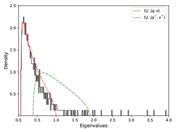
(a)

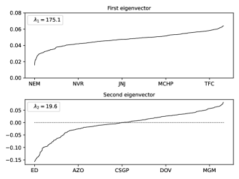
(b)

Figure 3: (Left) Eigenvalue distribution for the selected universe (black). Marcenko-Pastur density for $\hat{q}=6.97$ and $\hat{\sigma}^{2}=1$ (green). A fit obtained with an optimal pair $(q^{*},\sigma^{*})$ different from those associated with the training set for illustration purposes (red). (Right) Components of the first and second eigenvectors in ascending order.

With the chosen number of factors, a decomposition (as in Equation (12)) of standardized asset returns to the level of factors and residuals can be performed. In other words, the return of a stock $j\in\{1,\dots,433\}$ for a given date with the index $i\in\{1,\dots,3020\}$, $\bar{\mathbf{X}}_{i,j}$, can be expressed as the sum of a factor-based return $\mathbf{Y}_{i,j}=\mathbf{F}_{i,:}^{\top}\mathbf{P}_{j,1:16}$ and a residual return $\mathbf{Z}_{i,j}$. We adopt different modeling approaches for these components, as detailed in Section 3.2.2 and Section 3.2.4, based on the premise that factor-based returns are responsible for the dependence properties of returns, both cross-sectionally and across time, observed in financial markets [Cont, 2000].

A time-dependency analysis for a given $X(t)$ and lag $\tau\in\mathbb{Z}$ is usually performed using an autocorrelation function defined as

$$\rho_{X,(g_{1},g_{2})}(\tau)=\rho(g_{1}(X(t)),g_{2}(X(t+\tau))).$$

where $g_{1}:\mathbb{R}\rightarrow\mathbb{R}$ and $g_{2}:\mathbb{R}\rightarrow\mathbb{R}$ denote specific functions chosen according to the analysis in question and $\rho$ is the correlation function between two random variables.

For example, it is well documented that asset returns generally do not exhibit significant linear autocorrelation [Fama, 1970], unless analyzed at the microstructure level, with $\rho_{X,(x,x)}(\tau)\approx 0$, for $\tau>0$. On the other hand, some interesting non-linear relationships emerge for different choices of $g_{1}$ and $g_{2}$.

One notable phenomenon is the tendency for large price changes to be followed by other large price changes, also known as volatility clustering, as shown by the fact that $\rho_{X,(x^{2},x^{2})}$ or $\rho_{X,(|x|,|x|)}$ is significantly positive, at least for non-large $\tau$ [Ding et al., 1993]. Another important but less obvious relationship is known as the leverage effect [Bouchaud et al., 2001], which implies that negative returns lead to an increase in future volatility, often evidenced by $\rho_{X,(x,|x|)}(\tau)<0$, for $\tau>0$. Absence of this relationship for $\tau<0$ pointing out to the time-reversal assymetry in asset returns [Zumbach, 2007].

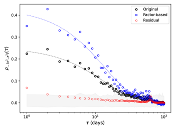
(a)

(b)

Figure 4: Median non-linear time dependence at the level of different components. Volatility clustering (left) and leverage effect (right) is confirmed in original asset returns and more strongly observed in factor-based returns with exponential $\propto ae^{-\gamma}$ and power law $\propto ax^{-\gamma}$ fits, respectively. Grey areas represent 95% bootstrap confidence interval for an i.i.d sample of the length of the training set from a standard Student-t with 3 degrees of freedom.

As illustrated in Figure 4, we carry out similar statistical analyses at the level of factor-based and residual returns, as well as at the level of original asset returns, to investigate how these two elements, which make up asset returns, contribute to the temporal dependence structure observed in financial markets. Firstly, although not shown in the figure, we found that the two components do not exhibit significant linear autocorrelation, nor do the asset returns themselves. However, more interesting insights are revealed from a non-linear analysis. Indeed, factor-based returns tend to show a more severe volatility clustering effect, while this effect is relatively negligible (but not totally absent) on the residual side. In the literature, the function $\rho_{X,(x^{2},x^{2})}$ is often found to be a slow-decay function as a power law with $\gamma\in[0.2,0.4]$, especially when computed on intraday data [Cont et al., 1997]. In our case, for daily returns, exponential function ($ae^{-\gamma}$) provides significantly better fits both for the original returns ($a=0.25$ and $\gamma=0.07$) and the factor-based returns ($a=0.42$ and $\gamma=0.07$).

Similar conclusion can be drawn regarding the leverage effect which is evident not only in the original asset returns ($a=-0.08$ and $\gamma=0.56$) but also and more in the components of factor-based returns ($a=-0.15$ and $\gamma=0.60$) with power law ($ax^{-\gamma}$) fits indicating a significant but fast-decay of this effect. As a result, we can argue that the observed inter-temporal properties of asset returns represent a diluted form of the more pronounced effects presented by factor-based returns, but noised by residuals, underlining the importance of capturing memory in factors in our modeling framework.

While the time-dependency properties of returns of a single asset are an area of interest for academics and practitioners, most financial problems are high-dimensional and require an understanding of the joint behavior of a large number of assets. The correlation matrix of asset returns is the main tool for analyzing these relationships linearly. It is often preferred over the covariance matrix for pure co-movement analysis, as it is unaffected by individual asset volatilities. For example, in the case of equities, stock returns within the same market tend to exhibit high correlations, with even higher correlations observed between stocks in the same sector, resulting in clusters within the correlation matrix.

Figure 5: Distribution of cross-asset correlations obtained from the lower triangle of the correlation matrix computed for different components.

However, it is fair to say that the roles of factor-based and residual returns in contributing to asset correlations are not necessarily the same although their impacts to the total variance are similar. As indicated in Section 3.2.1, the distribution of eigenvalues associated with residuals resembles the spectral distribution of a correlation matrix calculated on random entries. The fact that the correlations between asset returns are induced by a few factors forming factor-based returns is demonstrated in Figure 5 and Table 2 where we see that the correlations between residual returns are small and centered around zero. Figure LABEL:fig:correl_of_three_comps in Appendix LABEL:appendix:visual provides an illustration of the three correlation matrices computed on historical data.

	Cross-asset correlations
Original	0.39 [0.18, 0.63]
Factor-based	0.69 [0.34, 0.94]
Residual	0.00 [-0.07, 0.06]

Table 2: Median cross-asset correlations computed for different components with the inverval covering 95% of the cross-asset correlations.

In addition to inter-temporal and cross-asset dependencies, the marginal distributions of asset returns also exhibit unique properties. Among the most notable are asymmetry in gains and losses and the heavy-tailedness of the asset return distribution. The former is often characterized by the negative skewness of asset returns, indicating a tendency for more extreme downward movements than upward movements, with downward moves being less frequent. While kurtosis can provide insight into heavy-tailedness, a more nuanced analysis on losses involves estimating the tail-index $\gamma$ of the marginal distribution of asset returns using alternative estimators, such as Hill’s tail-index estimator:

$$\hat{\xi}(k)=\frac{1}{k}\sum_{i=1}^{k}\log{(-\mathbf{r}_{(i)})}-\log{(-\mathbf{r}_{(k)})}$$ (17)

where $\mathbf{r}_{(k)}$ denotes the $k^{th}$ order statistic of a given sample of asset returns $\mathbf{r}$. Loosely speaking, the parameter $k$, specified based on the sample size, sets the threshold beyond which it is believed the tail begins. However, the estimated value of $\hat{\xi}$ can be highly dependent on the choice of $k$. Therefore, it is common practice to compute it for different values of $k$. Intuitively, this estimator evaluates how losses beyond a certain quantile deviate from the selected level on average, offering an estimation of the heaviness of the left-tail where the tail-index is estimated by $\hat{\gamma}=1/\hat{\xi}$.

Figure 6: Distribution of the empirical skewness (left) and kurtosis (middle) of the 433 stocks for the different components. Median Hill’s index estimates of different components for different values of $k$ with the inverval covering 95% of the values across the universe (right). Estimates from a normal distribution are added for comparison.

Figure 6 provides some interesting insights into the marginal distributions of the different components of returns. First, factor-based returns appear to exhibit a consistent negative skewness for most assets, while skewness estimates for residual and original returns tend to vary around zero, although they can reach significantly high positive or negative levels. This suggests that the widely observed negative asymmetry in asset returns may be attributed more to common components that drive returns rather than being solely a feature of individual assets. However, the same argument may not hold for extreme returns and losses, as both components of asset returns exhibit particularly high kurtosis for almost all assets. A similar analysis focusing on the left tail can be carried out by estimating the tail index. Essentially, the well-known phenomenon of heavy tails in asset returns cannot be attributed solely to the presence of a single component, since the factor-based returns and residuals for the majority of stocks simultaneously exhibit this phenomenon in their distributions, as supported by Table 3.

	Skewness	Kurtosis	Tail Index
Original	-0.03 [-1.01 1.18]	11.8 [4.4 42.9]	2.84 [2.19 3.62]
Factor-based	-0.21 [-1.10 0.55]	13.8 [3.8 46.1]	2.91 [2.30 3.75]
Residual	0.10 [-1.82 2.21]	13.3 [4.0 64.2]	2.68 [1.99 3.67]

Table 3: Median values for different statistics at the level of different components across the universe with 95% confidence intervals in brackets.

In conclusion, the observations above serve as motivation for our approach to modeling asset returns from the perspective of two distinct components with differing characteristics. We have observed that most of the stylized facts of asset returns are present in the factor-based returns, sometimes more prominently, suggesting that they may warrant modeling using complex tools capable of capturing properties at both the temporal and cross-sectional levels. For the former, we use a memory of length of $s=63$ days, and for the latter, the cross-sectional properties are incorporated exogenously via the projection matrix $\hat{\bm{\beta}}=\mathbf{P}_{1:16}$.

Conversely, residuals can be treated as independent and identically distributed (i.i.d.) given the relative absence of linear and non-linear dependence over time, and the insignificant correlations. However, the model should still better account for their skewed and heavy-tailed nature, making a mixture of Student-t distributions a reasonable choice. For the sake of simplicity, we omit the asymmetry of residual returns and use a Student-t distribution (fixing $p=1$ in Equation (15)) and estimate the parameters for residuals of each asset using the maximum likelihood approach.

Recall from Section 3.2.3 that the selected factors are to be modeled by a smaller number of GANs trained on clusters of factors. In our numerical case, 16 factors are grouped into $n_{c}=3$ clusters based on 5 features. Specifically, these features include sample skewness and kurtosis computed on standardized daily factor returns, the eigenvalue associated with each factor, the volatility clustering score, and the leverage effect score computed over 63 days according to the following formula, with appropriate choices of $(g_{1},g_{2})$ being $(x^{2},x^{2})$ and $(x,x^{2})$, respectively:

$$\sum_{\tau=1}^{63}\rho_{F,(g_{1},g_{2})}(\tau)^{2}.$$ (18)

The agglomerative clustering algorithm applied to the above features results in the sets $\mathcal{C}_{1}=\{1\}$, $\mathcal{C}_{2}=\{3,6,12,14,15\}$ and $\mathcal{C}_{3}=\{2,4,5,7,8,9,10,11,13,16\}$. Therefore, 3 GANs with the same architecture and initial hyperparameters are trained using the training sets constructed based on the given clusterings. Details about the neural network architecture and training design are provided in Appendix LABEL:appendix:TCN, along with figures related to the evaluation of data generated by each of the three generators in Appendix LABEL:appendix:visual.

The training pipeline depicted in this subsection allows us to obtain the necessary parameters for the market generator as described by Equation (16). In the next section, we will assess the quality of the simulated data to determine whether it can effectively reproduce the learned properties present in asset returns.

4.2 A first look at simulated data

Although generative models have attracted attention and been used in a wide range of fields, there is no consensus on how to evaluate and validate what is produced by the trained model (see [Borji, 2018] for a review of evaluation measures). It is natural to expect different evaluation measures in different domains, but the lack of a common set of intra-domain measures makes it difficult to compare and horse-race models that have proved instrumental in the theoretical progress of deep learning over the last decade, as we have seen with ImageNet [Deng et al., 2009]. The considerable efforts being made to benchmark and evaluate LLMs also underline the importance of the issue [Hendrycks et al., 2020].

The absence of a generic evaluation procedure in finance is probably not due to the negligence of academics and practitioners, but to the specific character of the field. First of all, visual human inspection is extremely difficult, if not impossible, as opposed to the above mentioned cases of image-recognition and text-generation. Second of all, the nature of the generated data can be quite diverse, like market microstructure data [Cont et al., 2023], implied volatility surfaces [Vuletić and Cont, 2023], retail transactions [Lopez-Rojas and Axelsson, 2015], asset return / price processes and more.

The third point, which we touched on theoretically in Section 2.2 and which we shall explore in greater depth in Section 5, is the influence of the final application in the evaluation process, and the problematic nature of using the same measures even if the data generated is of the same type but comes from two distinct models designed for different purposes. In this subsection, we put this latter point aside and aim to perform a generic evaluation to assess the quality of the data generated by our market generator as rigorously as possible for a high-dimensional universe independent of the ultimate application, and show that we can obtain quite promising results from the market generator at least at first sight.

4.2.1 A marginal point of view

If we are in a context of generating multivariate asset returns, a generative model should ideally be capable of capturing the joint dynamics of the universe both cross-sectionally and inter-temporally. It is often more appropriate to carry out such an assessment with multiple evaluation steps, given the difficulty of doing a one-shot evaluation of the model as a whole.

First, we generate 100 simulated samples of the length of the training set, $n=3020$, from the market generator following the ideas developed in Section 2.1 regarding the balance between initial sample size and generated data. We begin by understanding whether the marginal distributions of asset returns in the generated scenarios are close to those observed historically, both in-sample (training set) and out-of-sample (test set). We use 1-Wasserstein distance as a measure of distance between simulated and historical distributions. For the empirical distributions, it boils down to a simple function of order statistics of the historical and simulated samples.

(a)

(b)

Figure 7: Wasserstein distances between simulated and historical samples based on different models. They are arranged in ascending order on the basis of distance from Gaussian fits for a clearer visualization.

Figure 7 illustrates the distances between the distribution of returns for each asset, in all scenarios, and the in-sample / out-of-sample distributions. For ease of comparison, the distances obtained by Gaussian and Student-t fits (obtained marginally for each asset using the training set) are also included. We see that the market generator provides better out-of-sample results on average, while Student-t distributions fit well in-sample but underperform out-of-sample due to likely overfitting issues, as shown in Table 4. The results look reasonably satisfactory in terms of marginal distributions for a modeling framework in which we do not learn directly from marginal distributions.

	In-sample	Out-of-sample
Gaussian	3.19 [2.02, 6.84]	2.69 [1.23, 7.59]
Student-t	0.65 [0.43, 1.24]	2.40 [1.21, 7.21]
Market Generator	1.45 [0.79, 4.35]	2.26 [1.07, 7.10]

Table 4: Median Wasserstein distance ($\times 10^{4}$) across the universe with the interval covering 95% of the scores.

To understand the model’s ability to reproduce inter-temporal effects at the asset level, we can consult the volatility clustering and leverage effect scores as defined in Equation (18). Figure 8 illustrates the scores computed on historical and simulated samples for each asset. It seems that the upward trend in in-sample scores is captured by the market generator up to a certain level, as shown by the increasing dispersion of the calculated scores and the upward trend in median scores for the simulated samples. Table 5 also shows that, in the market scenarios produced by the market generator, asset returns exhibit a time-dependency structure similar to that which we observe historically.

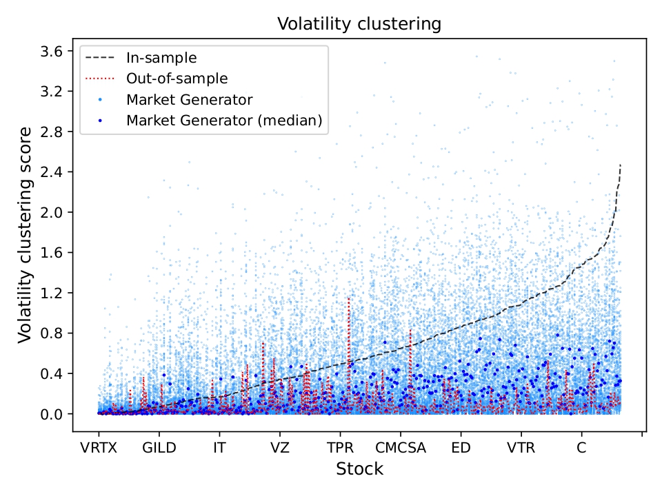
(a)

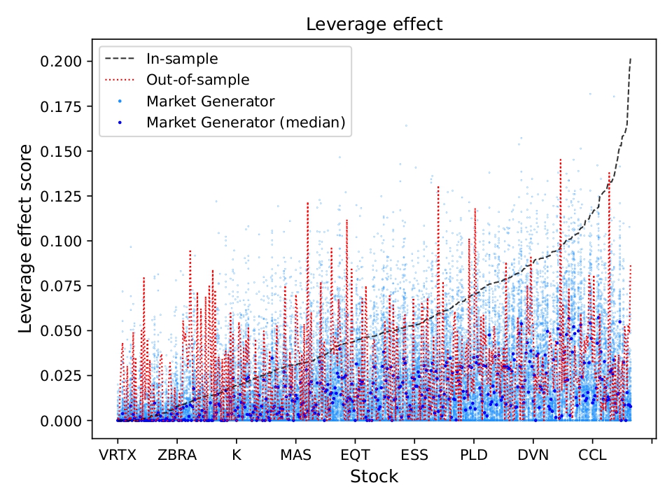
(b)

Figure 8: Volatility clustering and leverage effect scores computed on historical and simulated samples for each asset. They are arranged in ascending order on the basis of scores computed in-sample for a clearer visualization.

	Volatility Clustering	Leverage Effect
In-sample	53.88 [0.69, 174.34]	4.69 [0.0, 14.65]
Out-of-sample	3.60 [0.0, 42.94]	2.08 [0.0, 8.77]
Market Generator	14.66 [0.0, 63.77]	1.16 [0.0, 4.84]

Table 5: Median scores ($\times 10^{2}$) across the universe with the interval covering 95% of the scores.

Another aspect that deserves particular attention is the tail of asset return distributions, which are one of the most significant properties of asset returns, particularly when it comes to risk. Consequently, a market generator unable to generate extreme losses misses out one of the most crucial phenomena of asset returns.

A standard way to conduct an analysis of the left-tail of return distributions is to use Value-at-Risk (VaR) and Expected Shortfall. VaR at the level $\alpha\in(0,1)$ is simply a quantile of loss distribution of a real-valued random variable $X$ (regarded as a loss) and Expected Shortfall, on the other hand, is the average loss given that the loss exceeds $\text{VaR}_{\alpha}(X)$. Consequently, the similarity of VaR and Expected Shortfall (at high levels of $\alpha$) computed on historical and simulated samples, along with high kurtosis, should give an indication of the heavy-tailedness of the simulated marginal distributions, as summarized in Table 6 and illustrated in Figure 9.

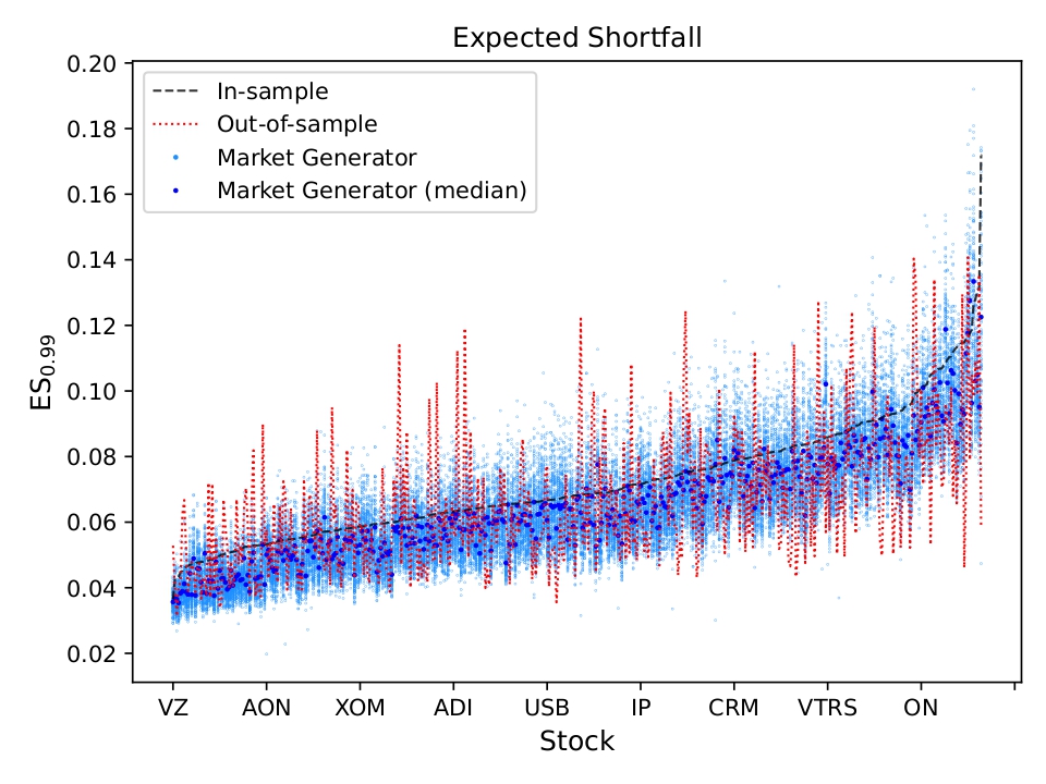
(a)

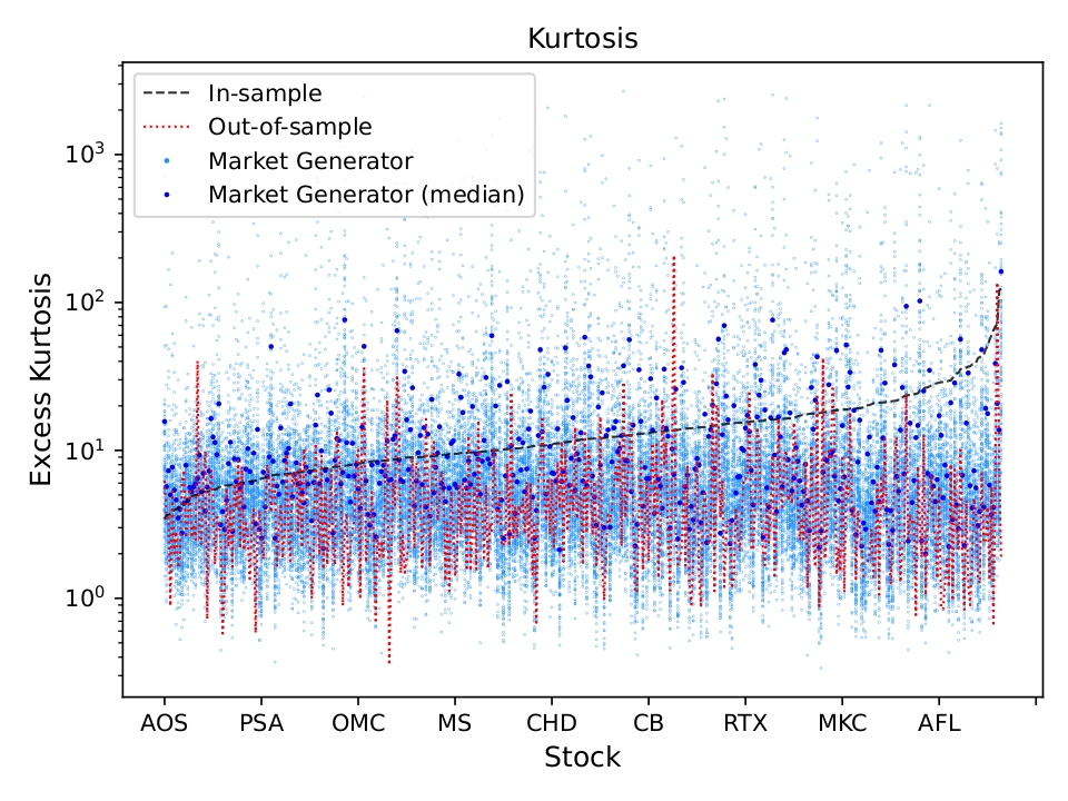
(b)

Figure 9: Expected Shortfall at the level 99% and kurtosis computed on historical and simulated samples for each asset. They are arranged in ascending order on the basis of values computed in-sample for a clearer visualization.

	In-sample	Out-of-sample	Market Generator
$\text{VaR}_{95\%}$	2.5 [1.7, 4.1]	2.7 [1.8, 4.8]	2.6 [1.8, 4.5]
$\text{VaR}_{99\%}$	4.6 [3.1, 7.5]	4.6 [3.0, 8.0]	4.5 [2.9, 7.5]
$\text{ES}_{95\%}$	4.0 [2.7, 6.6]	4.0 [2.7, 7.0]	3.9 [2.6, 6.6]
$\text{ES}_{99\%}$	6.8 [4.7, 11.4]	6.1 [3.9, 11.9]	6.2 [3.8, 10.2]
Kurtosis	11.8 [4.4, 42.9]	3.4 [0.9, 24.2]	4.7 [1.9, 14.2]

Table 6: Tail statistics across the universe with the interval covering 95% of the scores.

Until now, we have tried to verify whether we could get close to the marginal properties of individual asset returns by omitting the relationships between them, which are one of the most critical parts of multivariate modeling. To understand if at least linear relationships exist within the universe in a similar way to those observed historically, we analyze the distance between the sample correlation matrix calculated on simulated and historical returns :

$$\sum_{i=2}^{d-1}\sum_{j=1}^{i-1}(\mathbf{C_{sim}}_{i,j}-\mathbf{C_{hist}}_{i,j})^{2}$$

where $\mathbf{C_{sim}}$ denotes a sample correlation matrix calculated on a simulated sample and $\mathbf{C_{hist}}$ denotes a sample correlation matrix calculated on a historical sample (in-sample or out-of-sample). We also include two other estimators in our analysis to make the distance values meaningful. The first is what we call the one-factor model, which is simply a correlation matrix in which all correlations between assets are equal to the average correlations calculated in-sample. Although overly structured, such an approach is not completely unrealistic. The second correlation matrix estimator we consider is obtained using the covariance matrix estimate resulting from the Ledoit-Wolf estimator:

$$\tilde{\bm{\Sigma}}=(1-\gamma)\hat{\bm{\Sigma}}+\gamma\frac{\text{tr}(\hat{\bm{\Sigma}})}{d}\mathbf{I}_{d}$$

where $\hat{\bm{\Sigma}}$ is the sample covariance matrix and $\text{tr}(\hat{\bm{\Sigma}})$ is the trace of the covariance matrix. The optimal $\gamma$ can then be found such that the distance to the true covariance matrix is minimized (see [Ledoit and Wolf, 2003]).

	In-sample	Out-of-sample
One-Factor	13.27	20.98
Ledoit-Wolf	0.04	13.23
Market Generator	2.27 [0.79, 11.71]	16.39 [11.60, 112.10]

Table 7: Distance ($\times 10^{3}$) to historical correlation matrix for different estimators. Median value with 95% confidence interval for 100 realizations is shown for the market generator.

Table 7 shows the similarity of the correlation matrices to the historical ones obtained using different estimators. The Ledoit-Wolf estimator naturally produces the closest values to the in-sample correlations, since this information is already directly used. On the other hand, the market generator delivers competitive results to the Ledoit-Wolf estimator, particularly from an out-of-sample point of view. These findings underline the market generator’s ability to capture the correlation structure between asset returns. In Appendix LABEL:appendix:visual, we provide an illustration of correlation matrices computed in-sample and on synthetic data (see Figure LABEL:fig:corr_syn_vs_hist).

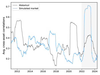
Figure 10: Evolution of average correlations (using a rolling window of one-year) between assets over time, calculated historically and on a generated sample of the same size. Shaded area represent the out-of-sample period.

In addition to the existence of a co-movement structure between asset returns, another important fact is that this structure is not static, but evolves over time. This means that correlations between assets are dynamic, and that the market has periods when correlations rise and fall, sometimes very suddenly. Increasing correlations between assets indicate a concentration of risk, reducing the scope for diversification within the universe. Such concentration is often monitored by examining the level of average correlations, with a high average indicating concentrated risk. Consequently, a market generator should also be tested for its ability to produce dynamic correlations as illustrated in Figure 10 using a simulated sample versus historical levels. This behavior arises from capturing volatility dynamics at the factor level, which induces dynamic correlations at the asset level despite the projection matrix being static.

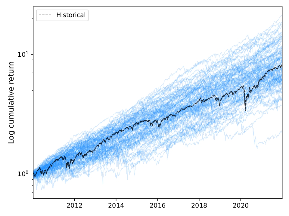
(a)

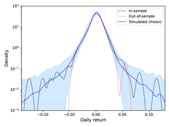
(b)

Figure 11: Returns of the equal-weighted portfolio computed on different samples.

4.2.2 Evaluation based on linear combinations

Given the challenge of evaluating each individual asset and the relationship between them, which we have attempted to achieve above, a natural idea would be to perform such an evaluation for a portfolio of these assets, in order to reduce the problem from high to one-dimensional. To this end, we consider an equally-weighted portfolio of the assets in question and calculate the returns of this portfolio historically and using our 100 simulated samples. We are now confronted with the problem of comparing two univariate time-series (simulated and historical) in a financially meaningful manner.

Although not a scientific investigation, but with the motivation that visual verification never hurts, Figure 11 illustrates the paths of the equal-weighted portfolio based on historical and simulated returns. The simulated trajectories look plausible and diffuse around the historical trajectory. The distribution of returns also appears to be on target, capturing quite well the heavy-tailed nature of portfolio returns.

A more systematic approach would be to compute certain statistics of interest to gain a deeper understanding of the results obtained for the simulated scenarios versus the in-sample and out-of-sample scenarios.

	Market Generator	In-sample	Out-of-sample
Ann. return (%)	19.86 [14.73, 26.19]	19.90	5.98
Ann. volatility (%)	18.53 [15.19, 22.52]	18.50	17.97
Sharpe ratio	1.09 [ 0.70 , 1.61]	1.08	0.33
Skewness	-0.45 [-0.95, 0.23]	-0.57	0.02
Kurtosis	11.40 [ 2.33, 30.78]	15.89	1.59
Maximum drawdown (%)	29.48 [15.45, 44.09]	38.00	19.45
$\text{VaR}_{95\%}$ (daily, %)	1.71 [1.39, 2.06]	1.66	1.67
$\text{VaR}_{95\%}$ (weekly, %)	3.75 [2.96, 4.50]	3.50	4.10
$\text{VaR}_{95\%}$ (monthly, %)	5.87 [3.75, 8.34]	5.52	8.09
$\text{VaR}_{99\%}$ (daily, %)	3.32 [2.63, 4.13]	3.19	3.06
$\text{VaR}_{99\%}$ (weekly, %)	7.10 [5.28, 8.68]	6.67	6.64
$\text{VaR}_{99\%}$ (monthly, %)	12.90 [7.72, 20.15]	13.09	10.39
$\text{ES}_{95\%}$ (daily, %)	2.80 [2.23, 3.47]	2.77	2.42
$\text{ES}_{95\%}$ (weekly, %)	5.90 [4.43, 7.20]	5.77	5.78
$\text{ES}_{95\%}$ (monthly, %)	10.16 [6.13, 14.73]	10.54	9.54
$\text{ES}_{99\%}$ (daily, %)	4.75 [3.43, 6.54]	4.80	3.47
$\text{ES}_{99\%}$ (weekly, %)	9.50 [6.83, 12.71]	10.25	8.72
$\text{ES}_{99\%}$ (monthly, %)	17.32 [9.81, 27.50]	21.96	11.66
Volatility clustering score	1.26 [0.34, 2.42]	1.69	0.43
Leverage effect score	0.11 [0.06, 0.19]	0.15	0.11

Table 8: Sample statistics of the equal-weighted portfolio computed on different samples with 95% confidence interval in brackets.

Table 8 lists some statistics that can summarize the behavior of portfolio returns and allow for an evaluation of the quality of the simulated samples. The market generator gives rather punctual (from an in-sample point of view) Sharpe ratio estimates, but this is natural since the market generator uses sample means and sample variances of individual assets estimated in-sample. More interesting results concern higher moments and tails. The negative skewness profile of the portfolio is well captured, although this phenomenon is absent out-of-sample, probably due to the fact that the test set is very limited, which also explains why in-sample and out-of-sample results differ substantially. Similar conclusions apply to kurtosis, although the mean value is lower than the in-sample value, but a wide confidence interval indicates the ability to generate various scenarios. Maximum drawdown being a path-dependent measure is at realistic levels on average where the confidence interval indicates the existence of scenarios where the strategy’s maximum drawdown can be (at least) as small as 15.45% and as large as 44.09% covering both in-sample and out-of-sample values. The VaR and Expected Shortfall calculated for different time horizons prove that the model not only works on a daily scale, but is also suitable for longer time horizons. Furthermore, the model’s performance does not decrease much for VaR and ES at high levels, demonstrating its ability to generate extreme losses. The volatility clustering and leverage effect scores indicate that these phenomena exist at the level of portfolio returns historically, which are also observed in the simulated scenarios. As these scores are not very revealing, we illustrate in Figure 12 how these properties are reproduced in the simulated samples.

In this section, we have carried out a general analysis to understand the behavior of our market generator and show that it can produce realistic scenarios according to some generic measures of evaluation. However, does it mean that it can now be used for the desired application safely? The next section is devoted to this question.

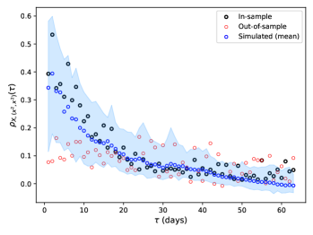
(a)

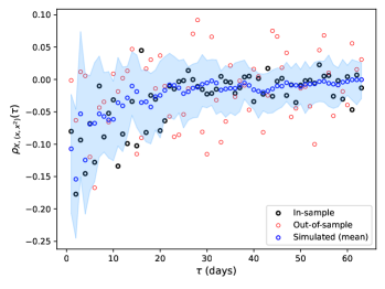
(b)

Figure 12: Inter-temporal properties of the equal-weighted portfolio computed on different samples.

5 In-depth evaluation of generative models

The previous section checked if the generative model produces known stylized facts. Nevertheless, the goal of a generator is not only to reproduce such facts, it targets a specific usage, a typical goal is to produce more data to tune hyperparameters of a downstream algorithm. Examples of downstream tasks are reinforcement learning algorithms or any portfolio construction algorithm. Thanks to Section 2.1, we know that it is useless to generate too many synthetic data points, but keeping it in a reasonable range, we can generate data points hoping it would help the downstream algorithm to generalize. In this spirit, underline it is known for long that adding noise to data provides some robustness to downstream optimizers (see [Bishop, 1995]), hence even if the virtue of a generative model is no more than to add noise a sound way to the information existing in the initial sample point, it would not be useless.

However, as mentioned, mimicking financial returns of a list of tradable instruments is exposed to a paradox. On the one hand the more the learning process of a generative model focuses on the distribution of the marginals (i.e. the returns of each instrument) and on the joined distribution of the returns (i.e. their covariance), the more it is attracted by the components of large variance of price moves. On the other hand, as soon as the generated trajectories are used to study portfolios, the exposure to these large variance carrying components is generally neutralised (or projected out by the process of portfolio construction). This is particularly true for long-short market neutral portfolios. As a consequence the focus of the generative model on the components with large variance is counterproductive. Our architecture aims to overcome this issue, and the only way to determine if it succeeds is by testing it within the ultimate use case: portfolio construction, and particularly in the case of backtesting long-short strategies.

5.1 The market generator for mean-reversion strategies: a comparison with block bootstrap

We propose to evaluate the quality of synthetic data on long-short portfolios invested on the cross-section of returns during the last $h$ days of the considered universe of stocks. The direction of the portfolio is made as if it is betting on the mean-reversion of the returns. In addition to the long-short case, we will also consider the long-only version of the strategy for benchmarking purposes.

The exact computations are detailed below, but first the reader should keep in mind stylized facts on the cross-section of returns: at short time scale (around one week, cf. for instance [Yeo and Papanicolaou, 2017]), the returns are meant to mean-revert, generating positive Sharpe ratio, then it slowly decreases down to the point it becomes the opposite of the cross-sectional momentum (one year plus one month, cf. [Asness et al., 2013]), then the sign of the profits and losses slowly inverts again to capture slow economic cycles (around a time scale of 3 years). This effect is visible on Figure 14. Beyond the test of one specific generative model, this effect can be considered as a valuable test for synthetic returns of universes of stocks.

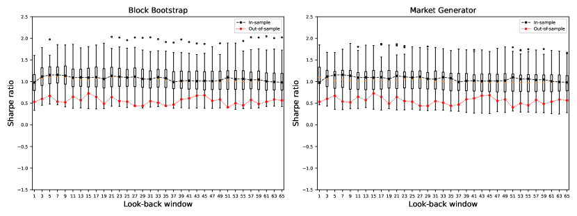
Figure 13: Boxplots of Sharpe ratios of the long-only mean-reversion strategy for different look-back window parameters $h$ backtested on samples from block bootstrap approach (left) and the market generator (right).

Details of the methodology.

More specifically, let us consider a case where the market generator will be used to capture the real shape of the Sharpe ratio scaling profile—a curve obtained by plotting the Sharpe ratio of a given strategy as a function of varying window size parameter $h$.

To implement the long-short mean-reversion strategy, we compute $h$-day returns for each asset in the universe, we rank them in descending order, short the first quintile and long the last quintile, assigning equal weight to each asset in both legs such that the portfolio is dollar-neutral. We also use an implementation lag of $\max(\frac{h}{10},1)$ days. Long-only version of the strategy corresponds to an equal-weighted portfolio of the last quintile, all other things being equal. We assume a daily rebalancing and no transaction costs. As mentioned, we want to observe the evolution of the Sharpe ratio for different $h$ under simulated scenarios.

We use the block bootstrap method to obtain confidence intervals for the statistics of strategies, preserving the intertemporal structure of stock returns [Carlstein, 1986]. As a consequence, block bootstrapped confidence intervals on historical returns can be considered as a baseline model to compare any generative model to.

We run the long-only and the long-short mean reversion strategies on 100 block-bootstrapped historical samples (using a window size of 63 days) and 100 simulated samples from the market generator of the size of the training set. For each sample, we test for $h\in\{1,3,5,\dots,65\}$. It means that for each $h$, we obtain an empirical distribution of Sharpe ratios which is illustrated in Figure 13 for the long-only strategy under both methods.

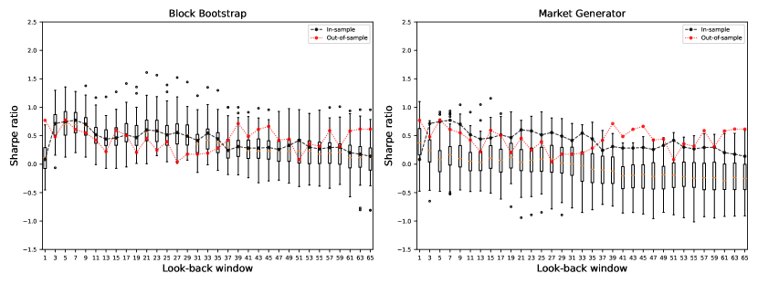
Figure 14: Boxplots of Sharpe ratios of the long-short mean-reversion strategy for different look-back window parameters $h$ backtested on samples from block bootstrap approach (left) and the market generator (right).

Long-Only Mean Reversion Long-Short Mean Reversion $h$ Block Boot. Market Gen. IS OoS Block Boot. Market Gen. IS OoS 1 0.99 [0.47, 1.35] 1.09 [0.54, 1.75] 0.98 0.53 0.11 [-0.32, 0.57] 0.38 [-0.36, 1.05] 0.08 0.77 5 1.09 [0.68, 1.60] 1.02 [0.56, 1.59] 1.15 0.67 0.70 [0.21, 1.23] 0.08 [-0.46, 0.83] 0.75 0.77 9 1.10 [0.67, 1.62] 1.03 [0.56, 1.60] 1.14 0.52 0.67 [0.30, 1.18] 0.10 [-0.38, 0.85] 0.70 0.55 13 1.05 [0.61, 1.62] 1.02 [0.58, 1.61] 1.10 0.57 0.45 [0.13, 0.82] 0.03 [-0.40, 0.56] 0.44 0.22 17 1.07 [0.62, 1.60] 1.04 [0.56, 1.55] 1.10 0.65 0.51 [0.17, 1.01] 0.07 [-0.36, 0.72] 0.51 0.51 21 1.10 [0.52, 1.65] 1.03 [0.56, 1.60] 1.13 0.64 0.56 [0.18, 1.11] 0.03 [-0.52, 0.75] 0.60 0.45 25 1.08 [0.54, 1.61] 1.05 [0.56, 1.67] 1.09 0.53 0.53 [0.13, 1.09] 0.09 [-0.45, 0.82] 0.51 0.39 29 1.07 [0.53, 1.60] 1.04 [0.57, 1.61] 1.06 0.44 0.51 [0.10, 1.00] 0.02 [-0.52, 0.70] 0.49 0.18 33 1.06 [0.55, 1.59] 1.00 [0.54, 1.58] 1.10 0.51 0.42 [0.03, 0.90] -0.03 [-0.64, 0.50] 0.55 0.19 37 0.99 [0.50, 1.58] 0.99 [0.52, 1.59] 0.99 0.47 0.30 [-0.11, 0.78] -0.10 [-0.67, 0.49] 0.24 0.42 41 1.01 [0.51, 1.57] 0.96 [0.52, 1.53] 1.02 0.61 0.24 [-0.16, 0.77] -0.21 [-0.76, 0.34] 0.28 0.49 45 1.00 [0.54, 1.58] 0.97 [0.52, 1.55] 1.02 0.68 0.22 [-0.22, 0.77] -0.18 [-0.79, 0.32] 0.29 0.66 49 0.99 [0.51, 1.59] 0.97 [0.52, 1.55] 1.02 0.59 0.22 [-0.22, 0.75] -0.19 [-0.81, 0.36] 0.33 0.44 53 1.01 [0.53, 1.58] 0.97 [0.53, 1.58] 1.06 0.50 0.23 [-0.27, 0.81] -0.22 [-0.77, 0.32] 0.30 0.36 57 0.99 [0.51, 1.56] 0.97 [0.50, 1.53] 1.04 0.57 0.20 [-0.26, 0.73] -0.24 [-0.76, 0.39] 0.29 0.59 61 0.99 [0.50, 1.52] 0.98 [0.49, 1.55] 1.01 0.53 0.11 [-0.36, 0.72] -0.29 [-0.84, 0.37] 0.20 0.58

Table 9: Median Sharpe ratios (with 95% confidence intervals in brackets) of the long-only and long-short mean-reversion strategies for different look-back window parameters $h$ backtested on samples from block bootstrap approach and the market generator along with in-sample (IS) and out-of-sample values (OoS).

Commenting the results.

As expected for the long-only portfolios since their PnL is driven by the directions carrying to most variance, the median values of the block bootstrap approach align closely with the in-sample Sharpe ratios, and the out-of-sample values falling within the 95% confidence intervals. Similarly, the market generator shows a coherent pattern, with the exception of small differences at small $h$, where the wide confidence intervals centered on the in-sample Sharpe ratios still include the out-of-sample values.

However, as expected again, the long-short case, less exposed to the first components of the PCA, as shown in Figure 14 and in Table 9, presents a different and more complex picture. The block bootstrap confidence intervals still move around the in-sample values, showing a clear upward trend up to $h=7$ and $h=9$ days, followed by a decline for larger $h$ values whereas the highest out-of-sample Sharpe ratio at $h=1$ falling outside of the confidence interval.

It is hence interesting to note that despite the structure of our specific market generator making its best to not solely focus on the first components of the PCA, but also on the ones with smaller variance: there is a better alignment of in-sample, out-of-sample and synthetic data for long-only portfolios, that are driven by these first components. Long-short portfolios, less exposed to these principal factors, exhibit more disagreement between in-sample, out-of sample and synthetic data. Block bootstrap on historical data is clearly closer to the history than what synthetic data can provide.

This trend seems absent in the scenarios generated by the market generator, where the median values are noticeably lower than historical levels. These results might raise concerns about the model’s ability to capture specific market behaviors, raising skepticism about its effectiveness for backtesting long-short strategies.

The difference between the properties of the investment strategy on historical data and synthetic data calls for a deeper analysis, conducted in the following subsection.

5.2 Testing for identifiability

Two analysis are conducted through this subsection:

• what is the likelihood of the Sharpe ratio scaling profile if we consider the synthetic data are the true generative model?

• If the true generative model is a known one, how easy it is for a market generator of the same family to capture its Sharpe ratio scaling profile?

We approach the first question regarding the analysis of the variance of the desired statistics by leveraging the market generator, which, as shown in previous sections, captures certain characteristics of financial markets. This allows us to generate samples of varying sizes, where the true (asymptotic) behavior of the long-short mean-reversion strategy is known. The key point here is to shed light to the standard error of the Sharpe ratio for a dynamic, long-short strategy applied to a high-dimensional universe. If the standard error is too high for the given size of the in-sample set, then even if a market generator produces results similar to those computed in-sample, the estimate might still be unreliable, as it could be far from the true value.

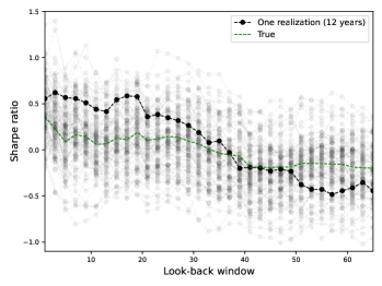
(a)

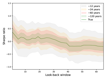
(b)

Figure 15: (Left) Sharpe ratio scaling profiles, computed on 100 simulated samples of the same size as the training set. One of the curves is randomly highlighted in bold. The true Sharpe ratios are represented by the green line. (Right) Sharpe ratio scaling profile, computed on 100 simulated samples of varying sizes to visualize the standard error as a function of the sample size using 95% confidence intervals.

$h$	12 years	24 years	60 years	120 years
1	0.44 (0.31)	0.41 (0.22)	0.39 (0.15)	0.36 (0.10)
5	0.15 (0.33)	0.11 (0.24)	0.11 (0.14)	0.09 (0.10)
9	0.17 (0.35)	0.16 (0.22)	0.16 (0.14)	0.14 (0.10)
13	0.09 (0.31)	0.07 (0.20)	0.09 (0.12)	0.06 (0.09)
17	0.12 (0.30)	0.11 (0.21)	0.13 (0.13)	0.11 (0.09)
21	0.08 (0.31)	0.10 (0.22)	0.11 (0.14)	0.10 (0.09)
25	0.12 (0.32)	0.15 (0.21)	0.16 (0.15)	0.15 (0.09)
29	0.08 (0.32)	0.09 (0.20)	0.11 (0.13)	0.09 (0.09)
33	-0.03 (0.32)	-0.00 (0.21)	0.02 (0.13)	0.01 (0.09)
37	-0.10 (0.31)	-0.07 (0.22)	-0.05 (0.14)	-0.05 (0.10)
41	-0.25 (0.29)	-0.21 (0.19)	-0.18 (0.12)	-0.19 (0.10)
45	-0.24 (0.29)	-0.21 (0.19)	-0.19 (0.12)	-0.19 (0.10)
49	-0.23 (0.29)	-0.20 (0.18)	-0.18 (0.12)	-0.19 (0.09)
53	-0.18 (0.29)	-0.16 (0.19)	-0.15 (0.12)	-0.15 (0.09)
57	-0.18 (0.30)	-0.16 (0.19)	-0.15 (0.13)	-0.15 (0.09)
61	-0.22 (0.29)	-0.19 (0.20)	-0.19 (0.12)	-0.19 (0.09)

Table 10: Mean Sharpe ratios (with standard errors in parentheses) for the long-short mean-reversion strategy applied to simulated samples of varying sizes (in years) generated by the market generator.

Let us recall the problem encountered at the end of Section 5.1 regarding the boxplots for the market generator not being centered around in-sample estimates and exhibiting a different trend. Although this observation might be significant, we cannot be certain whether the Sharpe ratios computed on simulated scenarios are also far from the true values associated with the underlying data-generating process, which remains unknown in reality.

To gain insight into this dilemma, we synthetically replicate the reality by generating 100 simulated samples, each with the same size as the training set (3020 points, approximately 12 years of daily returns). Imagine that one of these samples represents the realized history we have in reality. Unlike in reality, where the true Sharpe ratio scaling profile is unknown, here we know the true values that a generative model should capture, yet we only have access to a realized history that may diverge from the actual truth. The left-hand chart in Figure 15 illustrates this issue. A good model trained using the sample that generates the black curve should actually be able to produce scenarios that result in curves or boxplots centered around the green line. The wide cluster of points around the true values highlights the insufficiency of the initial sample size in accurately representing the true statistics. This variance indicates that the sample may not be large enough to reliably reflect the underlying truth for the desired statistics.

We can also assess the number of data points required for in-sample statistics to become reliable and representative of the true values, thus allowing us to effectively evaluate the generative model. The right-hand chart in Figure 15 and Table 10 show how the accuracy of in-sample statistics in approximating the true values improves with increasing sample size. These results may highlight the challenge of optimizing long-short strategies with relatively small data sets using generative models.

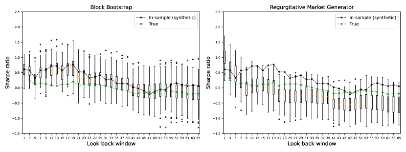
Figure 16: Boxplots of Sharpe ratios of the long-short mean-reversion strategy for different look-back window parameters $h$ backtested on samples from the block bootstrap approach (left) and the regurgitative market generator (right).

$h$	Block Boot.	Reg. Market Gen.	IS	True
1	0.61 [0.07, 1.00]	1.06 [0.29, 1.60]	0.61	0.45
5	0.30 [-0.12, 0.83]	0.42 [-0.29, 1.13]	0.32	0.11
9	0.45 [-0.08, 1.15]	-0.08 [-0.64, 0.61]	0.60	0.13
13	0.58 [0.16, 1.17]	0.07 [-0.46, 0.63]	0.72	0.06
17	0.61 [0.06, 1.15]	0.05 [-0.58, 0.57]	0.74	0.12
21	0.37 [-0.11, 1.07]	-0.25 [-0.83, 0.25]	0.53	0.07
25	0.25 [-0.28, 1.00]	-0.25 [-0.93, 0.27]	0.32	0.13
29	0.32 [-0.25, 0.93]	-0.26 [-0.94, 0.32]	0.41	0.09
33	0.23 [-0.31, 0.88]	-0.17 [-0.86, 0.35]	0.29	0.01
37	0.13 [-0.40, 0.86]	-0.27 [-0.87, 0.24]	0.15	-0.06
41	-0.03 [-0.66, 0.60]	-0.52 [-1.12, -0.05]	0.02	-0.19
45	-0.12 [-0.79, 0.57]	-0.53 [-1.05, -0.00]	-0.09	-0.16
49	-0.15 [-0.78, 0.61]	-0.54 [-1.10, 0.03]	-0.12	-0.17
53	-0.07 [-0.84, 0.69]	-0.45 [-1.05, 0.17]	-0.06	-0.10
57	-0.06 [-0.94, 0.68]	-0.45 [-1.04, 0.25]	0.16	-0.13
61	-0.07 [-0.95, 0.63]	-0.61 [-1.13, 0.12]	0.06	-0.21

Table 11: Median Sharpe ratios (with 95% confidence intervals in brackets) of the long-short mean-reversion strategies for different look-back window parameters $h$, backtested on samples from both the block bootstrap approach and the regurgitative market generator. The regurgitative market generator was trained on a synthetic sample (IS) generated by the market generator where the true Sharpe ratios are known (True).

Concerning identifiability, let us focus on the second question that is related to the ability of the market generator to identify itself at the level of the particular characteristics of a benchmark strategy. Explicitly, what we propose is as follows: Take your generative model and simulate a sample of the same size as the training set used to train it. Then, using the same training pipeline and architecture, train a second generative model—let us call it the regurgitative market generator—on this synthetic sample, for which we already know the true underlying characteristics. Ideally, the regurgitative market generator should be able to infer something about this truth from the limited dataset provided. As a result, the characteristics of benchmark portfolios computed on samples from the regurgitative market generator should align with the true values rather than simply replicating the in-sample estimates. If your market generator cannot even identify its own characteristics from a limited sample, there is little hope that it can capture the underlying truth in real-world scenarios, where the generative model likely differs from the architecture of the market generator.

Above process is not designed to validate good models but to detect bad ones. The aim is to subject the generative model to a test it must pass to be considered further for use. The goal is to understand whether the regurgitative market generator can capture some of the true characteristics of the benchmark strategy.

Figure 16 illustrates this test and highlights the limitations of the block bootstrap for generalizations. First, we observe that the block bootstrap is strongly dependent on the training set, following the in-sample trend closely. In contrast, the regurgitative market generator appears to extract some insights about the underlying truth of Sharpe ratio scaling profile for increasing $h$, avoiding the V-shaped trend observed in the in-sample estimates for small $h$. However, it does not align perfectly with the true levels (as evidenced by the median values not matching the true values), which could lead to concerns about the model’s effectiveness. Table 11 shows the Sharpe ratio scaling profiles under both the block bootstrap and the regurgitative market generator, providing additional context for evaluating whether the generative pipeline produces valuable results.

6 Conclusion

In this paper, we first emphasized the importance of the initial sample size when training generative models. It is crucial to recognize that generating more synthetic data does not necessarily improve the accuracy of estimates, and it can remove uncertainty from the analysis, leading to biased conclusions. We then explained why simply applying a generative model to financial data for portfolio construction may not work. This issue is fundamentally tied to the principles of both portfolio construction and generative modeling. Consequently, such a use case requires careful engineering of the generative pipeline. Next, we introduced the engineering approach we propose to create a generative pipeline that is more suitable for portfolio construction. Our approach demonstrates promising results for the specific example of US stocks based on conventional evaluation measures. Additionally, we provided insights into the origins of stylized facts commonly observed in asset returns within this universe. Lastly, we highlighted that the evaluation of generative models should always be aligned with the intended application. We emphasize the importance of assessing the standard error of computed statistics and proposed a test based on retraining the model using its own generated data—a test that every model should pass before being applied further.

References

- [Aaronson et al., 1996] Aaronson, J., Burton, R., Dehling, H., Gilat, D., Hill, T., and Weiss, B. (1996). Strong laws for l-and u-statistics. Transactions of the American Mathematical Society, 348(7):2845–2866.
- [Aghabozorgi et al., 2015] Aghabozorgi, S., Shirkhorshidi, A. S., and Wah, T. Y. (2015). Time-series clustering–a decade review. Information Systems, 53:16–38.
- [Arjovsky et al., 2017] Arjovsky, M., Chintala, S., and Bottou, L. (2017). Wasserstein GAN. arXiv:1701.07875 [cs, stat].
- [Asness et al., 2013] Asness, C. S., Moskowitz, T. J., and Pedersen, L. H. (2013). Value and momentum everywhere. The journal of finance, 68(3):929–985.
- [Assefa, 2020] Assefa, S. (2020). Generating Synthetic Data in Finance: Opportunities, Challenges and Pitfalls. SSRN Electronic Journal.
- [Ben Arous et al., 2019] Ben Arous, G., Mei, S., Montanari, A., and Nica, M. (2019). The landscape of the spiked tensor model. Communications on Pure and Applied Mathematics, 72(11):2282–2330.
- [Bentkus et al., 2009] Bentkus, V., Jing, B.-Y., and Zhou, W. (2009). On normal approximations to u-statistics. Annals of Probability, 37(6):2174–2199.
- [Berkowitz, 1999] Berkowitz, J. (1999). A coherent framework for stress-testing. Available at SSRN 181931.
- [Bishop, 1995] Bishop, C. M. (1995). Training with noise is equivalent to tikhonov regularization. Neural computation, 7(1):108–116.
- [Black, 1986] Black, F. (1986). Noise. The Journal of Finance, 41(3):528–543.
- [Borji, 2018] Borji, A. (2018). Pros and Cons of GAN Evaluation Measures. arXiv:1802.03446 [cs].
- [Bouchaud et al., 2001] Bouchaud, J.-P., Matacz, A., and Potters, M. (2001). Leverage effect in financial markets: The retarded volatility model. Physical Review Letters, 87(22):228701.
- [Boyd et al., 2024] Boyd, S., Johansson, K., Kahn, R., Schiele, P., and Schmelzer, T. (2024). Markowitz portfolio construction at seventy. arXiv preprint arXiv:2401.05080.
- [Boyle, 1977] Boyle, P. P. (1977). Options: A Monte Carlo approach. Journal of Financial Economics, 4(3):323–338.
- [Broadie and Glasserman, 1996] Broadie, M. and Glasserman, P. (1996). Estimating security price derivatives using simulation. Management Science, 42(2):269–285.
- [Brown, 2020] Brown, T. B. (2020). Language models are few-shot learners. arXiv preprint arXiv:2005.14165.
- [Bryzgalova et al., 2019] Bryzgalova, S., Pelger, M., and Zhu, J. (2019). Forest Through the Trees: Building Cross-Sections of Stock Returns. SSRN Electronic Journal.
- [Buehler et al., 2020] Buehler, H., Horvath, B., Lyons, T., Arribas, I. P., and Wood, B. (2020). A data-driven market simulator for small data environments. arXiv preprint arXiv:2006.14498.
- [Capponi and Lehalle, 2023] Capponi, A. and Lehalle, C.-A. (2023). Machine learning and data sciences for financial markets. Technical report, Cambridge University Press.
- [Caprioli et al., 2023] Caprioli, S., Cagliero, E., and Crupi, R. (2023). Quantifying Credit Portfolio sensitivity to asset correlations with interpretable generative neural networks. arXiv:2309.08652 [cs, q-fin].
- [Carlstein, 1986] Carlstein, E. (1986). The use of subseries values for estimating the variance of a general statistic from a stationary sequence. The Annals of Statistics, pages 1171–1179.
- [Carriere, 1996] Carriere, J. F. (1996). Valuation of the early-exercise price for options using simulations and nonparametric regression. Insurance: Mathematics and Economics, 19(1):19–30.
- [Chen and Shao, 2007] Chen, L. H. and Shao, Q.-M. (2007). Normal approximation for nonlinear statistics using a concentration inequality approach. Bernoulli, 13(2):581–599.
- [Cont, 2000] Cont, R. (2000). Empirical properties of asset returns: stylized facts and statistical issues. Quantitative Finance.
- [Cont, 2010] Cont, R. (2010). Stylized properties of asset returns. Encyclopedia of Quantitative Finance.
- [Cont et al., 2023] Cont, R., Cucuringu, M., Kochems, J., and Prenzel, F. (2023). Limit order book simulation with generative adversarial networks. Available at SSRN 4512356.
- [Cont et al., 2022] Cont, R., Cucuringu, M., Xu, R., and Zhang, C. (2022). Tail-GAN: Nonparametric Scenario Generation for Tail Risk Estimation. arXiv:2203.01664 [q-fin].
- [Cont et al., 1997] Cont, R., Potters, M., and Bouchaud, J.-P. (1997). Scaling in stock market data: stable laws and beyond. In Scale Invariance and Beyond: Les Houches Workshop, March 10–14, 1997, pages 75–85. Springer.
- [Da Silva and Shi, 2019] Da Silva, B. and Shi, S. S. (2019). Style transfer with time series: Generating synthetic financial data. arXiv preprint arXiv:1906.03232.
- [de Meer Pardo, 2019] de Meer Pardo, F. (2019). Enriching financial datasets with generative adversarial networks. MS thesis, Delft University of Technology, The Netherlands.
- [de Prado, 2020] de Prado, M. M. L. (2020). Machine Learning for Asset Managers. Cambridge University Press.
- [Dempster et al., 1977] Dempster, A. P., Laird, N. M., and Rubin, D. B. (1977). Maximum likelihood from incomplete data via the em algorithm. Journal of the royal statistical society: series B (methodological), 39(1):1–22.
- [Deng et al., 2009] Deng, J., Dong, W., Socher, R., Li, L.-J., Li, K., and Fei-Fei, L. (2009). Imagenet: A large-scale hierarchical image database. In 2009 IEEE conference on computer vision and pattern recognition, pages 248–255. Ieee.
- [Desai et al., 2021] Desai, A., Freeman, C., Wang, Z., and Beaver, I. (2021). TimeVAE: A Variational Auto-Encoder for Multivariate Time Series Generation. arXiv:2111.08095 [cs].
- [Ding et al., 1993] Ding, Z., Granger, C. W., and Engle, R. F. (1993). A long memory property of stock market returns and a new model. Journal of Empirical Finance, 1(1):83–106.
- [Dogariu et al., 2022] Dogariu, M., Ştefan, L.-D., Boteanu, B. A., Lamba, C., Kim, B., and Ionescu, B. (2022). Generation of realistic synthetic financial time-series. ACM Trans. Multimedia Comput. Commun. Appl., 18(4).
- [Eckerli, 2021] Eckerli, F. (2021). Generative Adversarial Networks in finance: an overview. SSRN Electronic Journal.
- [Ericson et al., 2024] Ericson, L., Zhu, X., Han, X., Fu, R., Li, S., Guo, S., and Hu, P. (2024). Deep generative modeling for financial time series with application in var: A comparative review. arXiv preprint arXiv:2401.10370.
- [Fama, 1970] Fama, E. F. (1970). Efficient capital markets: A review of theory and empirical work. The Journal of Finance, 25(2):383–417.
- [Feizi et al., 2017] Feizi, S., Farnia, F., Ginart, T., and Tse, D. (2017). Understanding gans: the lqg setting. arXiv preprint arXiv:1710.10793.
- [Flaig and Junike, 2023] Flaig, S. and Junike, G. (2023). Validation of machine learning based scenario generators. arXiv:2301.12719 [q-fin].
- [Fu et al., 2022] Fu, W., Hirsa, A., and Osterrieder, J. (2022). Simulating financial time series using attention. arXiv preprint arXiv:2207.00493.
- [Glasserman, 2004] Glasserman, P. (2004). Monte Carlo Methods in Financial Engineering, volume 53. Springer.
- [Goerg, 2015] Goerg, G. M. (2015). The lambert way to gaussianize heavy-tailed data with the inverse of tukey’sh transformation as a special case. The Scientific World Journal, 2015(1):909231.
- [Goodfellow et al., 2014] Goodfellow, I. J., Pouget-Abadie, J., Mirza, M., Xu, B., Warde-Farley, D., Ozair, S., Courville, A., and Bengio, Y. (2014). Generative Adversarial Networks. arXiv:1406.2661 [cs, stat].
- [Hendrycks et al., 2020] Hendrycks, D., Burns, C., Basart, S., Zou, A., Mazeika, M., Song, D., and Steinhardt, J. (2020). Measuring massive multitask language understanding. arXiv preprint arXiv:2009.03300.
- [Henry-Labordere, 2019] Henry-Labordere, P. (2019). Generative models for financial data. Available at SSRN 3408007.
- [Hertz, 1964] Hertz, D. B. (1964). Risk analysis in capital investment. Harvard Business Review, 42:95–106.
- [Hinton and Sejnowski, 1983] Hinton, G. E. and Sejnowski, T. J. (1983). Optimal perceptual inference. In Proceedings of the IEEE conference on Computer Vision and Pattern Recognition, volume 448, pages 448–453. Citeseer.
- [Ho et al., 2020] Ho, J., Jain, A., and Abbeel, P. (2020). Denoising diffusion probabilistic models. Advances in Neural Information Processing Systems, 33:6840–6851.
- [Hoeffding, 1948] Hoeffding, W. (1948). A Class of Statistics with Asymptotically Normal Distribution. The Annals of Mathematical Statistics, 19(3):293 – 325.
- [Hornik et al., 1989] Hornik, K., Stinchcombe, M., and White, H. (1989). Multilayer feedforward networks are universal approximators. Neural networks, 2(5):359–366.
- [Horvath et al., 2023] Horvath, B., Gonzalez, A. M., and Pakkanen, M. S. (2023). Harnessing quantitative finance by data-centric methods. Machine Learning and Data Sciences for Financial Markets: A Guide to Contemporary Practices, page 265.
- [Issler and Vahid, 1996] Issler, J. V. and Vahid, F. (1996). Common cycles in macroeconomic aggregates. mimeo.
- [Jäckel, 2002] Jäckel, P. (2002). Monte Carlo Methods in Finance, volume 5. John Wiley & Sons.
- [Jamshidian and Zhu, 1996] Jamshidian, F. and Zhu, Y. (1996). Scenario simulation: Theory and methodology. Finance and Stochastics, 1:43–67.
- [Kaastra and Boyd, 1996] Kaastra, I. and Boyd, M. (1996). Designing a neural network for forecasting financial and economic time series. Neurocomputing, 10(3):215–236.
- [Kantorovich, 1960] Kantorovich, L. V. (1960). Mathematical methods of organizing and planning production. Management Science, 6(4):366–422.
- [Kaplan et al., 2020] Kaplan, J., McCandlish, S., Henighan, T., Brown, T. B., Chess, B., Child, R., Gray, S., Radford, A., Wu, J., and Amodei, D. (2020). Scaling laws for neural language models. arXiv preprint arXiv:2001.08361.
- [Karras et al., 2020] Karras, T., Aittala, M., Hellsten, J., Laine, S., Lehtinen, J., and Aila, T. (2020). Training generative adversarial networks with limited data.
- [Kim et al., 2019] Kim, Y., Kang, D., Jeon, M., and Lee, C. (2019). Gan-mp hybrid heuristic algorithm for non-convex portfolio optimization problem. The Engineering Economist, 64(3):196–226.
- [Kingma and Welling, 2013] Kingma, D. P. and Welling, M. (2013). Auto-encoding variational bayes. arXiv preprint arXiv:1312.6114.