Sequentializing a Test: Anytime Validity is Free

Abstract

An anytime valid sequential test permits us to peek at observations as they arrive. This means we can stop, continue or adapt the testing process based on the current data, without invalidating the inference. Given a maximum number of observations $N$, one may believe that this benefit must be paid for in terms of power when compared to a conventional test that waits until all $N$ observations have arrived. Our key contribution is to show that this is false: for any valid test based on $N$ observations, we derive an anytime valid sequential test that matches it after $N$ observations. In addition, we show that the value of the sequential test before a rejection is attained can be directly used as a significance level for a subsequent test. We illustrate this for the $z$-test. There, we find that the current state-of-the-art based on log-optimal $e$-values can be obtained as a special limiting case that replicates a $z$-test with level $\alpha\to 0$ as $N\to\infty$.

Keywords: sequential testing, anytime validity, $e$-values, sequential $z$-test.

1 Introduction

Suppose that we are to observe $N$ i.i.d. observations $X^{N}:=X_{1},\dots X_{N}$. We are interested in testing the null hypothesis that each data point $X_{i}$ is sampled from distribution $\mathbb{P}$, against the alternative hypothesis that it is sampled from distribution $\mathbb{Q}$. Traditionally, we wait until all $N$ observations have been collected, and then perform a test which either rejects the hypothesis or not.

It is common to model such a test as a function $\phi_{N}$ from the data $X^{N}$ to the interval $[0,1]$, where its value indicates the probability with which we should subsequently reject the hypothesis. This means $\phi_{N}=1$ is a rejection, $\phi_{N}=0$ is a non-rejection, and $\phi_{N}=1/2$, say, means that we may subsequently reject with probability 1/2.

It is near-universal practice to use a test that is valid at some level of significance $\alpha>0$. This means that the probability that it rejects the null hypothesis is at most $\alpha$ if the null hypothesis is true. This can be translated to a condition on the expectation of $\phi_{N}$:

$$\mathbb{P}(\phi_{N}\text{ rejects})=\mathbb{E}^{\mathbb{P}}[\phi_{N}]\leq\alpha.$$ (1)

An unfortunate feature of this traditional approach is that we must sit on our hands and wait until all $N$ observations have arrived. Naively, one may believe that we can simply use the test $\phi_{n}(X^{n})$ after the arrival of every new observation and stop as soon as we find a rejection. However, this naive procedure is not valid, as the probability that one of the tests $\phi_{1}(X^{1}),\dots,\phi_{N}(X^{N})$ rejects at some point $n\leq N$ is typically much larger than $\alpha$. That is, the sequence of tests $\phi_{1}(X^{1}),\dots,\phi_{N}(X^{N})$ is not anytime valid:

$$\mathbb{E}^{\mathbb{P}}[\phi_{\tau}]\leq\alpha,$$ (2)

for some data-dependent (‘stopping’) time $\tau$.

Following seminal work by Robbins, Darling, Wald and others in the previous century, there has recently been a renaissance in anytime valid testing (Howard et al., 2021; Shafer, 2021; Ramdas et al., 2023; Grünwald et al., 2023). Such anytime valid sequential tests are typically of a different form than traditional tests. The currently most popular sequential test is based on log-optimal e-values, and equals $\alpha\textnormal{LR}_{n}\wedge 1$ at every observation $n$, where $\textnormal{LR}_{n}$ denotes the likelihood ratio between $\mathbb{Q}$ and $\mathbb{P}$ of the $n$ observations.

At time $N$, this sequential test is usually substantially less powerful than the optimal ‘Neyman-Pearson’ test. For example, in a standard normal location setting where we test $\mu=0$ against $\mu=.3$ with $N=100$ observations, the $z$-test rejects with probability 91% while this sequential test rejects at any time $n\leq N$ with probability just 79%. Moreover, this power comparison is very generous towards the sequential test, as it uses oracle knowledge of the alternative $\mu$, whereas the $z$-test does not. If we were to sequentially learn the alternative with the MLE, then its power is just 47%.

1.1 Sequentializing a test

The large power gap between the state-of-the-art and the traditional Neyman-Pearson test seems to be generally viewed as the cost of anytime validity. Indeed, this additional anytime validity must surely come at the cost of power!

Our key contribution is to show that this is false: anytime validity can be obtained for free. In particular, for any valid test $\phi_{N}$ we show how to construct a sequence of tests $\phi_{1}^{\prime},\dots\phi_{N}^{\prime}$ that is anytime valid and matches $\phi_{N}$ at the end: $\phi_{N}^{\prime}=\phi_{N}$.

Moreover, the test is of a very simple form: it simply equals the conditional probability that $\phi_{N}$ will reject, given the current data $X^{n}$ under null hypothesis $\mathbb{P}$:

$$\phi_{n}^{\prime}=\mathbb{P}(\phi_{N}\text{ rejects}\mid X^{n}).$$

We can immediately see that $\phi_{0}^{\prime}=\mathbb{P}(\phi_{N}\text{ rejects})$, which is bounded by $\alpha$ if $\phi_{N}$ is valid. Moreover, $\phi_{N}^{\prime}=\mathbb{P}(\phi_{N}\text{ rejects}\mid X^{N})=\phi_{N}$ by construction. The anytime validity follows from the fact that $\phi_{n}^{\prime}$ is a martingale, so that Doob’s optional stopping theorem implies

$$\mathbb{E}[\phi_{\tau}^{\prime}]\leq\phi_{0}^{\prime},$$ (3)

for every stopping time $\tau$. We show how this can be generalized to composite hypotheses which contain more than one distribution, and to other filtrations that describe the available information at time $n$.

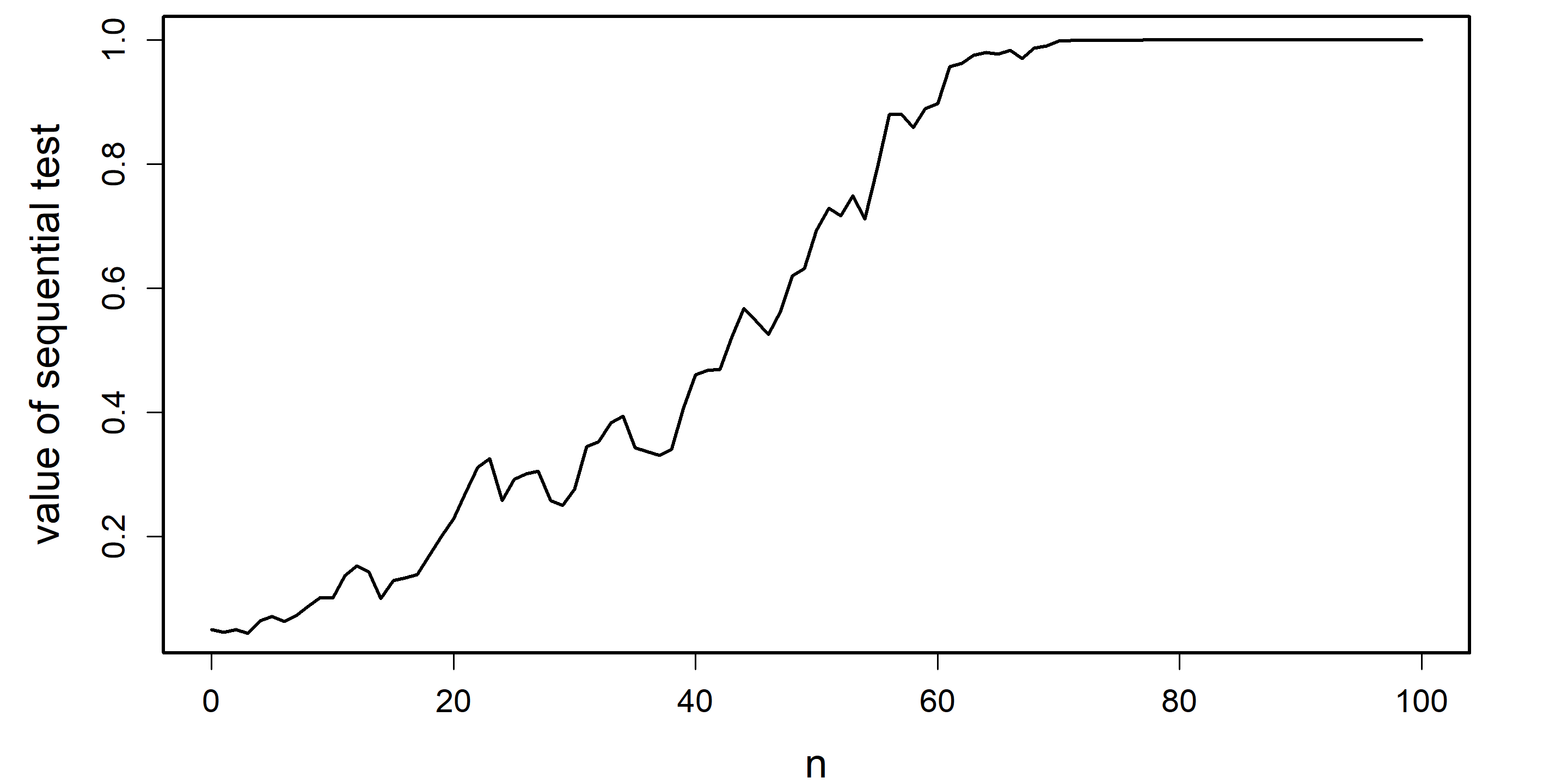
Figure 1: Illustration of the sequential $z$-test over $100$ observations sampled from $\mathcal{N}(.3,1)$.

We illustrate this for the one-sided $z$-test, of which we display an illustration in Figure 1 for a typical sample of i.i.d. normal data with a power 91% at $N=100$ observations. What we observe in the figure, is that the test seems to reject the null hypothesis well before all $100$ observations have arrived. This is false: as the normal distribution is unbounded there always remains a slim chance at $n$ observations that the remaining $N-n$ observations will be extremely large and negative so that $\phi_{N}$ will not reject. This means that $\phi_{n}^{\prime}<1$ for all $n<N$, so that the test technically never rejects before time $N$. However, while we may technically not attain a rejection before time $N$, this does not seem to be important in practice as $\phi_{n}^{\prime}$ may be extremely close to 1 even if $n\ll N$. In this example, $\phi_{n}^{\prime}$ is numerically indistinguishable from 1 by our R script for $n\geq 93$ and exceeds 0.999 for $n\geq 76$.

1.2 Sequential test as significance level

The fact that we typically have $\phi_{n}^{\prime}<1$ for $n<N$ may feel somewhat discomforting: what is the point of being able to peek at all these observations if it never leads us to reject the null hypothesis early?

This leads us to a remarkably elegant new insight: we can halt the sequential test after $n$ observations and use the value of $\phi_{n}^{\prime}$ as our level of significance from observation $n+1$ onward. The resulting procedure remains anytime valid at the original level $\alpha$. This means we can interpret $\phi_{n}^{\prime}$ as the level of significance with which we can continue testing.

For example, suppose that $N=1000$ and $\phi_{n}^{\prime}=.99$ after just $n=30$ observations. Then, we may abort the sequential test and conduct a new test at significance level $\alpha_{n}^{*}=\phi_{n}^{\prime}=.99$ based on the, say, $N^{*}=10$ next observations, which will then likely lead to a rejection.

More generally, after $n$ observations we can start a different sequential test from observation $n+1$ onward, which we initialize with a the significance level equal to $\phi_{n}^{\prime}$. For example, if $\phi_{n}^{\prime}$ is close to 1 after only a few observations, then it may be interesting to switch over to another sequential test that finalizes after $N^{-}\ll N$ observations so that we can quickly obtain a rejection. On the other hand, if $\phi_{n}$ remains far from 1 after many observations have come in, then we may want to switch over to another sequential test that finalizes after $N^{+}\gg N$ observations to still hope for a rejection.

In general, this permits us to glue sequential tests together in a highly flexible manner, and gives a new interpretation of a test that takes value in $(0,1)$ as the ‘current level of significance’.

In case we are in need of an immediate decision after $n$ observations and cannot afford any more observations, then a valid decision can always be obtained by rolling the dice and rejecting with probability $\phi_{n}^{\prime}$.

The value of $\phi_{n}^{\prime}$ can also be directly interpreted as evidence against the null hypothesis. Indeed, Koning (2024a) note that this is equivalent to directly interpreting a distribution on the outcome space $\{\text{not reject},\text{reject}\}$, and also equivalent to directly interpreting an $e$-value as evidence.

1.3 Comparison to log-optimal e-values

As mentioned, the currently most popular sequential test is based on log-optimal e-values and equals $\alpha\textnormal{LR}_{n}\wedge 1$. This object is deeply related to the likelihood ratio. Indeed, starting from this sequential test $\alpha\text{LR}_{n}\wedge 1$, we can rescale it by $1/\alpha$ to $\text{LR}_{n}\wedge 1/\alpha$ and then choose $\alpha=0$ to obtain the likelihood ratio $\text{LR}_{n}$. This means that following the likelihood ratio directly can be interpreted as following a kind of level $\alpha=0$ test (Koning, 2024a).

In Section 5.2, we study the likelihood ratio process for i.i.d. draws for the Gaussian location hypotheses $\mathbb{P}=\mathcal{N}(0,\sigma^{2})$ vs $\mathbb{Q}=\mathcal{N}(\mu,\sigma^{2})$. We find that it can be interpreted as a sequential $z$-test based on $N$ draws at level $\alpha_{N}=\exp\left\{-\tfrac{N\mu^{2}}{2\sigma^{2}}\right\}$ in the limit as $N\to\infty$.

This means that if we are using the likelihood ratio process, we are implicitly tracking the rejection probability under $\mathbb{P}$ that a $z$-test for large $N$ and small $\alpha$ will reject. This gives another motivation for the likelihood ratio process, beyond the typical Kelly-betting argument that it maximizes the long-run expected growth rate (Shafer, 2021; Grünwald et al., 2023).

1.4 Related literature

Inference based on e-values is often contrasted to traditional inference based on tests and $p$-values, and frequently described as an entirely different paradigm. Anytime validity is then viewed as a natural property of the e-value paradigm, which is not available in the traditional paradigm (Ramdas et al., 2022; Grünwald et al., 2023). One of our contributions is to dispel this myth, by showing that sequential testing also comes naturally to tests.

Koning (2024a) unifies e-values and traditional tests, and argues that e-values are merely tests viewed at a different (better) scale. Using this interpretation, our work gives new insights into sequential testing with e-values: we find that multiplying sequential e-values is equivalent to gluing together tests by initializing the second test with a level equal to the first test.

Our approach relies on constructing a Doob martingale towards the test we wish to ‘sequentialize’. We are not the first to use such a Doob martingale in the context of anytime valid sequential testing. Indeed, it is also featured as a technical tool in a proof in Section 6.3 of Ramdas et al. (2022) and underlies the construction of time uniform concentration inequalities in Howard et al. (2020). However, to the best of our knowledge, we are the first to propose to actively construct anytime valid sequential tests in this manner.

Given the simple interpretation of $\phi_{n}^{\prime}$ as the probability that the replicated test $\phi_{N}$ will reject under $\mathbb{P}$, it is not surprising that we are not the first to use this object. Indeed, it also appears in a stream of literature initiated by Lan et al. (1982), who propose to reject whenever $\phi_{n}^{\prime}>\gamma$ for some pre-specified $\gamma$. This induces a sequential test $\phi_{n}^{\gamma}=\mathbb{I}\{\phi_{n}^{\prime}>\gamma\}$, which they show has a Type I error bounded by $\alpha/\gamma$. In subsequent literature, $\phi_{n}^{\prime}$ appears under the name conditional power, and is also used as a diagnostic tool to stop for futility (Lachin, 2005).

Compared to this stream of literature, we use $\phi_{n}^{\prime}$ differently. We avoid pre-specifying a threshold $\gamma$, and instead directly interpret $\phi_{n}^{\prime}$ or use it as a subsequent significance level to obtain an early rejection. This reveals that the name ‘conditional size’ may be more appropriate than ‘conditional power’. Moreover, we extend to composite hypotheses and any type of filtration: not necessarily i.i.d. nor even independent data.

Lastly, to the best of our knowledge, this stream of work has gone unnoticed in the current renaissance in anytime valid sequential testing: we only discovered it by searching the web after establishing the elegant interpretation as a conditional rejection probability. As a result, another one of our contributions is to connect these two streams of literature. This allows us to employ the rich mathematical toolbox that has recently been developed in the e-value and anytime validity literature.

2 Example: $z$-test

In this section, we briefly illustrate our methods in the context of a one-sided $z$-test. Suppose that $X_{1},\dots,X_{N}$ are independently drawn from the normal distribution $\mathcal{N}(\mu,1)$, with mean $\mu\in\mathbb{R}$. Then, the uniformly most powerful test for testing the null hypothesis $\mu\leq 0$ against the alternative hypothesis $\mu>0$ is the one-sided $z$-test.

At a given level $\alpha>0$, this test equals

$$\phi_{N}=\mathbb{I}\left\{N^{-1/2}\sum_{i=1}^{N}X_{i}>z_{1-\alpha}\right\},$$

where $z_{1-\alpha}$ is the $\alpha$ upper-quantile of the distribution $\mathbb{P}=\mathcal{N}(0,1)$. As a consequence, for $n<N$, its induced sequential test is given by

$$\phi_{n}^{\prime} =\mathbb{P}\left(\frac{1}{\sqrt{N}}\sum_{i=1}^{N}X_{i}>z_{1-\alpha}\mid X_{1},\dots,X_{n}\right)$$

$$=\mathbb{P}\left(\frac{1}{\sqrt{N}}\sum_{i=n+1}^{N}X_{i}>z_{1-\alpha}-\tfrac{1}{\sqrt{N}}\sum_{i=1}^{n}x_{i}\right)$$

$$=\Phi\left(\frac{\sum_{i=1}^{n}x_{i}-\sqrt{N}z_{1-\alpha}}{\sqrt{N-n}}\right)$$

where $\Phi$ is the CDF of the standard normal distribution $\mathcal{N}(0,1)$, and $x_{1},\dots,x_{n}$ are the realizations of $X_{1},\dots,X_{n}$. If $n=N$ this is poorly defined as denominator equals zero, but still works if we define $y/0$ as $+\infty$ if $y>0$ and as $-\infty$ if $y<0$.

To interpret the sequential test $\phi_{n}^{\prime}$ and compare it to the $z$-test at time $N$, $\phi_{N}$, it helps to write it as

$$\Phi\left(\frac{N^{-1/2}\sum_{i=1}^{n}x_{i}-z_{1-\alpha}}{\sqrt{\frac{N-n}{N}}}\right).$$ (4)

Here, we see that the the argument of $\Phi$ is simply the difference between the current progress on the test statistic $N^{-1/2}\sum_{i=1}^{n}x_{i}$ and the critical value $z_{1-\alpha}$, divided by square-root of the proportion of observations that remain. This means that the denominator inflates the progress compared to the critical value if we have fewer observations left. If no observations remain, the progress is inflated to either $+\infty$ or $-\infty$, depending on whether the test statistic exceeds the critical value or not. As $\Phi(\infty)=1$ and $\Phi(-\infty)=0$, the function $\Phi$ then translates this to a rejection or non-rejection of the hypothesis.

In Example 1 we explain why this sequential test is anytime valid for the entire composite hypothesis $\mu\leq 0$, but to do this it helps to first give our technical results.

3 Technical results

Let $\mathcal{X}$ be our sample space equipped with some sigma-algebra $\mathcal{F}$. Moreover, suppose we have some filtration $(\mathcal{F}_{n})_{n\in\mathbb{N}}$, where $\mathcal{F}_{n}\subseteq\mathcal{F}$ describes the available information $\mathcal{F}_{n}$ at time $n\in\mathbb{N}$. For simplicity, let $\mathcal{F}_{0}=\{\emptyset,\mathcal{X}\}$ represent the information set before any data has been observed, so that we can write the expectation $\mathbb{E}[\,\cdot\,]$ for the conditional expectation given $\mathcal{F}_{0}$, $\mathbb{E}[\,\cdot\mid\mathcal{F}_{0}]$.

We define a hypothesis $H$ as a collection of probability measures $\mathbb{P}\in H$ on $\mathcal{X}$. Without loss of generality, we follow Koning (2024a) by modeling a level $\alpha\geq 0$ test as a map $\varepsilon_{\alpha}:\mathcal{X}\to[0,1/\alpha]$. For $\alpha>0$, a test on the traditional $[0,1]$-scale can be recovered through $\phi_{\alpha}=\alpha\varepsilon_{\alpha}$. For $\alpha=0$, this is more general. A test $\varepsilon_{\alpha}$ is said to be valid for $H$ if

$$\sup_{\mathbb{P}\in H}\mathbb{E}^{\mathbb{P}}[\varepsilon_{\alpha}]\leq 1.$$ (5)

Such a valid test $\varepsilon_{\alpha}$ is also known as an e-value, bounded to $[0,1/\alpha]$ (Shafer, 2021; Vovk and Wang, 2021; Howard et al., 2021; Ramdas et al., 2023; Grünwald et al., 2023; Koning, 2024b, a).

A sequence of level $\alpha$ tests $(\varepsilon_{n})_{n\in\mathbb{N}}$ adapted to the filtration $(\mathcal{F}_{n})_{n\in\mathbb{N}}$ is said to be anytime valid for $H$ if

$$\sup_{\mathbb{P}\in H}\mathbb{E}^{\mathbb{P}}[\varepsilon_{\tau}]\leq 1,$$ (6)

for every stopping time $\tau$ adapted to $(\mathcal{F}_{n})_{n\in\mathbb{N}}$. An anytime valid sequence of tests $(\varepsilon_{n})_{n\leq N}$ has recently also been named an e-process (Ramdas et al., 2022).

We first present the result for simple null hypotheses, which contain only a single distribution, as it permits a more insightful proof. We then follow it by the more general result for composite null hypotheses, which may contain multiple distributions.

Theorem 1 (Simple hypotheses).

Let $H$ be a simple hypothesis: $H=\{\mathbb{P}\}$. Let the level $\alpha\geq 0$ test $\varepsilon$ be $\mathcal{F}$-measurable. Define the sequence of level $\alpha$ tests $(\varepsilon_{n})_{n\in\mathbb{N}}$ as

$$\varepsilon_{n}=\mathbb{E}^{\mathbb{P}}[\varepsilon\mid\mathcal{F}_{n}].$$ (7)

Then, $\mathbb{E}^{\mathbb{P}}[\varepsilon_{\tau}]\leq\mathbb{E}^{\mathbb{P}}[\varepsilon]=\varepsilon_{0}$, for every stopping time $\tau$ adapted to $(\mathcal{F}_{n})_{n\in\mathbb{N}}$. As a consequence, if $\varepsilon$ is valid for $H$, then $(\varepsilon_{n})_{n\in\mathbb{N}}$ is anytime valid for $H$. Moreover, if $\varepsilon$ is $\mathcal{F}_{N}$-measurable, $N\in\mathbb{N}$, then $\varepsilon_{n}=\varepsilon$ for all $n\geq N$.

Proof.

By the law of iterated expectations,

$$\mathbb{E}^{\mathbb{P}}[\varepsilon_{n}\mid\mathcal{F}_{n-1}] =\mathbb{E}^{\mathbb{P}}[\mathbb{E}^{\mathbb{P}}[\varepsilon\mid\mathcal{F}_{n}]\mid\mathcal{F}_{n-1}]$$

$$=\mathbb{E}^{\mathbb{P}}[\varepsilon\mid\mathcal{F}_{n-1}]$$

$$=\varepsilon_{n-1},$$

so that $(\varepsilon_{n})_{n\in\mathbb{N}}$ is a non-negative martingale. Hence, by Doob’s optional stopping theorem for non-negative martingales, we have

$$\mathbb{E}^{\mathbb{P}}[\varepsilon_{\tau}]\leq\mathbb{E}^{\mathbb{P}}[\varepsilon],$$

for every stopping time $\tau$.

Finally, if $\varepsilon$ is $\mathcal{F}_{N}$-measurable, then $\varepsilon_{N}=\mathbb{E}^{\mathbb{P}}[\varepsilon\mid\mathcal{F}_{N}]=\varepsilon$. As a result, $\varepsilon_{n}=\varepsilon$ for all $n\geq N$ as $(\mathcal{F}_{n})_{n\in\mathbb{N}}$ is a filtration. ∎

For the setting with a composite null hypothesis $H$, we do not replicate a single test but a test for each distribution $\mathbb{P}$ in the hypothesis. In case of the one-sided $z$-test, this would be the one-sided $z$-test for every $\mu\leq 0$.

Theorem 2 (Composite hypotheses).

Let the level $\alpha\geq 0$ tests $\varepsilon^{\mathbb{P}}$ be $\mathcal{F}$-measurable, for every $\mathbb{P}\in H$. Define the sequence of level $\alpha$ tests $(\varepsilon_{n})_{n\in\mathbb{N}}$ as

$$\varepsilon_{n}=\operatorname*{ess\,inf}_{\mathbb{P}\in H}\mathbb{E}^{\mathbb{P}}[\varepsilon^{\mathbb{P}}\mid\mathcal{F}_{n}].$$ (8)

Then,

$$\sup_{\tau\in\mathcal{T}}\sup_{\mathbb{P}\in H}\mathbb{E}^{\mathbb{P}}[\varepsilon_{\tau}]\leq\sup_{\mathbb{P}\in H}\mathbb{E}^{\mathbb{P}}[\varepsilon^{\mathbb{P}}],$$

where $\mathcal{T}$ is a collection of stopping times adapted to the filtration. As a consequence, if $\varepsilon^{\mathbb{P}}$ is valid for $\mathbb{P}$, then $(\varepsilon_{n})_{n\in\mathbb{N}}$ is anytime valid for $H$. Moreover, if every $\varepsilon^{\mathbb{P}}$ is $\mathcal{F}_{N}$-measurable, $N\in\mathbb{N}$, then $\varepsilon_{n}=\operatorname*{ess\,inf}_{\mathbb{P}\in H}\varepsilon^{\mathbb{P}}$ for all $n\geq N$.

Proof.

We have

$$\sup_{\tau\in\mathcal{T}}\sup_{\mathbb{P}\in H}\mathbb{E}^{\mathbb{P}}[\varepsilon_{\tau}] =\sup_{\mathbb{P}\in H}\sup_{\tau\in\mathcal{T}}\mathbb{E}^{\mathbb{P}}[\varepsilon_{\tau}]$$

$$=\sup_{\mathbb{P}\in H}\sup_{\tau\in\mathcal{T}}\mathbb{E}^{\mathbb{P}}\left[\operatorname*{ess\,inf}_{\mathbb{P}^{\prime}\in H}\mathbb{E}^{\mathbb{P}^{\prime}}[\varepsilon^{\mathbb{P}^{\prime}}\mid\mathcal{F}_{\tau}]\right]$$

$$\leq\sup_{\mathbb{P}\in H}\sup_{\tau\in\mathcal{T}}\mathbb{E}^{\mathbb{P}}\left[\mathbb{E}^{\mathbb{P}}\left[\varepsilon^{\mathbb{P}}\mid\mathcal{F}_{\tau}\right]\right]$$

$$=\sup_{\mathbb{P}\in H}\mathbb{E}^{\mathbb{P}}[\varepsilon^{\mathbb{P}}].$$

If $\varepsilon$ is $\mathcal{F}_{N}$-measurable, then

$$\varepsilon_{N} =\operatorname*{ess\,inf}_{\mathbb{P}\in H}\mathbb{E}^{\mathbb{P}}[\varepsilon^{\mathbb{P}}\mid\mathcal{F}_{N}]=\operatorname*{ess\,inf}_{\mathbb{P}\in H}\varepsilon^{\mathbb{P}}.$$

∎

As a corollary to Theorem 2, we can also use a single test by choosing $\varepsilon^{\mathbb{P}}=\varepsilon$ for every $\mathbb{P}\in H$. The advantage here is that we only need to specify a single test $\varepsilon$, and that the resulting sequential test $(\varepsilon_{n})_{n\in\mathbb{N}}$ always hits $\varepsilon$ at time $N$. The downside is that the sequential test may not be practically useful, and may be of the form $0,0,\dots,0,\varepsilon$. For example, this happens if we plug-in the one-sided $z$-test for $\mu=0$ if the hypothesis is that $\mu\leq 0$. This does not happen if we apply Theorem 2.

Corollary 1 (Composite with single test).

Let

$$\varepsilon_{n}=\operatorname*{ess\,inf}_{\mathbb{P}\in H}\mathbb{E}^{\mathbb{P}}[\varepsilon\mid\mathcal{F}_{n}],$$

where $\varepsilon$ is $\mathcal{F}$-measurable. Then,

$$\sup_{\tau\in\mathcal{T}}\sup_{\mathbb{P}\in H}\mathbb{E}^{\mathbb{P}}[\varepsilon_{\tau}]\leq\sup_{\mathbb{P}\in H}\mathbb{E}^{\mathbb{P}}[\varepsilon].$$

Hence, if $\varepsilon$ is valid for $H$, then $(\varepsilon_{n})_{n\in\mathbb{N}}$ is anytime valid for $H$. Moreover, if $\varepsilon$ is $\mathcal{F}_{N}$-measurable then $\varepsilon_{n}=\varepsilon$ for all $n\geq N$.

Remark 1 (e-processes and infimums).

While the infimum in (8) may seem unnecessarily conservative, Ramdas et al. (2022) show that an e-process can be equivalently defined as some stochastic process that is upper bounded by a $\mathbb{P}$-non-negative (super)martingale for every $\mathbb{P}\in H$. Moreover, they find that any admissible e-process for $H$ appears as the essential infimum of e-processes for $\mathbb{P}\in H$. Hence, taking the infimum is natural to anytime valid sequential tests.

A helpful observation here is that the tests $\varepsilon^{\mathbb{P}}$ in Theorem 2 are individually not valid for the composite hypothesis $H$, but only for the individual distributions $\mathbb{P}\in H$.

Remark 2 (Doob martingale).

In the existing literature on anytime valid inference, the standard strategy to build anytime valid sequential tests is to propose a sequence $(\varepsilon_{n})_{n\in\mathbb{N}}$ of tests and then show that this constitutes a martingale. Our approach here turns this around: we start with some target test $\varepsilon$, from which we then deduce a sequence of tests $(\varepsilon_{n})_{n\in\mathbb{N}}$ by conditioning on the filtration. For the simple hypothesis setting, this is approach is also known as Doob’s martingale of $\varepsilon$.

Example 1 (One-sided $z$-test composite).

Here, we show that the one-sided $z$-test as in Section 2 is indeed obtained if we plug-in the one-sided $z$-test for every $\mu\leq 0$ into Theorem 2. The one-sided $z$-test for $\mu$ at level $\alpha>0$ on the $[0,1]$-scale equals

$$\phi^{\mu}=\mathbb{I}\left\{\frac{1}{\sqrt{N}}\sum_{i=1}^{N}X_{i}>z_{1-\alpha}+\sqrt{N}\mu\right\}.$$

As $\mu\leq 0$, we have $\phi^{0}=\inf_{\mu\leq 0}\phi^{\mu}$. Next, using $\mathbb{E}^{\mu}$ and $\mathbb{P}^{\mu}$ to denote the expectation and probability under $\mathcal{N}(\mu,1)$, we have for $n<N$

$$\phi_{n}^{\mu} =\mathbb{E}^{\mu}[\phi^{\mu}\mid X_{1},\dots,X_{n}]$$

$$=\mathbb{P}^{\mu}\left(\sum_{i=n+1}^{N}X_{i}>N^{1/2}z_{1-\alpha}+N\mu-\sum_{i=1}^{n}x_{i}\right)$$

$$=\mathbb{P}^{0}\left(\sum_{i=n+1}^{N}(X_{i}+\mu)>N^{1/2}z_{1-\alpha}+N\mu-\sum_{i=1}^{n}x_{i}\right)$$

$$=\mathbb{P}^{0}\left(\sum_{i=n+1}^{N}X_{i}>N^{1/2}z_{1-\alpha}+n\mu-\sum_{i=1}^{n}x_{i}\right)$$

$$=\Phi\left(\frac{N^{-1/2}\sum_{i=1}^{n}x_{i}-z_{1-\alpha}-nN^{-1/2}\mu}{\sqrt{\frac{N-n}{N}}}\right),$$

which is the same as (4), but with an extra term involving $nN^{-1/2}\mu$ in the numerator. Note that the argument of $\Phi$ is decreasing in $\mu$. As $\mu\leq 0$, this implies $\inf_{\mu\leq 0}\phi_{n}^{\mu}=\phi_{n}^{0}$, which is indeed the sequential $z$-test as derived in Section 2. Moreover, as $\phi^{\mu}$ is valid for $\mathcal{N}(\mu,1)$, the sequential test is valid for the composite hypothesis $\mu\leq 0$ by Theorem 2.

4 Seamlessly gluing sequential tests

In the introduction, we stated that after $n^{*}$, say, observations we may start a new sequential test that we initialize with significance level equal to the value of our current sequential test $\phi_{n^{*}}^{\prime}$. In this section, we explain why ‘gluing’ together two anytime valid sequential tests in this manner yields an overall sequential test that is anytime valid. Moreover, in Remark 4, we explain how this gives an new interpretation to multiplying sequential e-values.

Suppose that $(\phi_{n}^{\prime})_{n\in\mathbb{N}}$ is an anytime valid sequential test at level $\alpha$ adapted to the filtration $(\mathcal{F}_{n})_{n\in\mathbb{N}}$. As $(\phi_{n}^{\prime})_{n\in\mathbb{N}}$ is anytime valid, this sequential test stopped at $n^{*}$ is valid, since anytime validity means that

$$\sup_{\mathbb{P}\in H}\mathbb{E}^{\mathbb{P}}[\phi_{\tau}^{\prime}]\leq\alpha,$$

for every stopping time $\tau$. Now, at time $n^{*}$, let us initialize some new $\mathcal{F}$-measurable test $\phi^{*}$ that is valid at level $\phi_{n^{*}}^{\prime}$:

$$\sup_{\mathbb{P}\in H}\mathbb{E}^{\mathbb{P}}[\phi^{*}\mid\mathcal{F}_{n^{*}}]\leq\phi_{n^{*}}^{\prime}.$$

Then, we have that the overall procedure including this test $\phi^{*}$ is valid, because

$$\sup_{\mathbb{P}\in H}\mathbb{E}^{\mathbb{P}}[\phi^{*}]=\sup_{\mathbb{P}\in H}\mathbb{E}^{\mathbb{P}}[\mathbb{E}^{\mathbb{P}}[\phi^{*}\mid\mathcal{F}_{n^{*}}]]\leq\sup_{\mathbb{P}\in H}\mathbb{E}^{\mathbb{P}}[\phi_{n^{*}}^{\prime}]\leq\alpha.$$

Moreover, we can apply Theorem 2 to design a sequential test $(\phi_{n}^{*})_{n\geq n^{*}}$ from $n^{*}$ onward that tests towards $\phi^{*}$:

$$\phi_{n}^{*}=\operatorname*{ess\,inf}_{\mathbb{P}\in H}\mathbb{E}^{\mathbb{P}^{\prime}}[\phi^{*}\mid\mathcal{F}_{n}],$$

for $n\geq n^{*}$.

The resulting procedure seamlessly ‘glues’ together two sequential tests: the resulting sequence of tests

$$\phi_{1}^{\prime},\dots,\phi_{n^{*}}^{\prime},\phi_{n^{*}+1}^{*},\dots$$

is anytime valid at level $\alpha$. The gluing happens at time $n^{*}$, where $\phi_{n^{*}}^{\prime}=\phi_{n^{*}}^{*}$, which is obtained by choosing $\phi_{n^{*}}^{\prime}$ as the starting significance level of the second sequential test.

Remark 3 (Gluing two tests).

While we framed the discussion above in terms of gluing two sequences of tests, we can also use this to glue two tests. Indeed, after conducting a valid level $\alpha$ test $\phi$, we may follow it with some new test $\phi^{*}$ on new data that is valid at significance level $\phi$. This yields a combined test that is valid at level $\alpha$.

Tests which take value in $\{0,1\}$, which are common in practice, are not well-suited to be used as the first test $\phi$ because initializing the second test with significance level 0 is useless.

Remark 4 (Relationship to multiplying e-values).

We can perform the same exercise on the evidence $[0,1/\alpha]$-scale as in Section 3. There, we find this is equivalent to multiplying sequentially valid tests.

To show this, we repeat the same steps on the evidence scale where we substitute in $\varepsilon_{n}^{\prime}=\phi_{n}^{\prime}/\alpha$ and $\varepsilon^{*}=\phi^{*}/\phi_{n^{*}}^{\prime}$.

As $(\varepsilon_{n}^{\prime})_{n\in\mathbb{N}}$ is anytime valid (sometimes called an ‘e-process’), stopping it at time $n^{*}$ is valid, because anytime validity means that

$$\sup_{\mathbb{P}\in H}\mathbb{E}^{\mathbb{P}}[\varepsilon_{\tau}^{\prime}]\leq 1,$$

for every stopping time $\tau$. Now, at time $n^{*}$ we initialize some $\mathcal{F}$-measurable test $\varepsilon^{*}$ that is valid at level $\alpha\varepsilon_{n^{*}}^{\prime}$:

$$\sup_{\mathbb{P}\in H}\mathbb{E^{\mathbb{P}}}[\varepsilon^{*}\mid\mathcal{F}_{n^{*}}]\leq 1.$$

As a consequence, we have that the product of $\varepsilon_{n^{*}}^{\prime}$ and $\varepsilon^{*}$ is valid:

$$\sup_{\mathbb{P}\in H}\mathbb{E}^{\mathbb{P}}[\varepsilon_{n^{*}}^{\prime}\varepsilon^{*}] =\sup_{\mathbb{P}\in H}\mathbb{E}^{\mathbb{P}}[\varepsilon_{n^{*}}^{\prime}\mathbb{E^{\mathbb{P}}}[\varepsilon^{*}\mid\mathcal{F}_{n^{*}}]]$$

$$\leq\sup_{\mathbb{P}\in H}\mathbb{E}^{\mathbb{P}}[\varepsilon_{n^{*}}^{\prime}]\leq 1.$$

Moreover, this product is of level $\alpha$, since $\varepsilon_{n^{*}}^{\prime}\varepsilon^{*}=\phi_{n^{*}}^{\prime}/\alpha\phi^{*}/\phi_{n^{*}}^{\prime}=\phi^{*}/\alpha:\mathcal{X}\to[0,1/\alpha]$.

5 Link log-optimal tests / e-values

5.1 Log-optimal and likelihood ratio process

To prepare for our result that interprets the likelihood ratio process as a sequentialized Neyman-Pearson test, we first discuss some background on log-optimal tests (e-values) and likelihood ratio processes.

Let us again consider tests $\varepsilon$ on the $[0,1/\alpha]$-scale, for testing the simple hypothesis $\mathbb{P}$ against $\mathbb{Q}$. In traditional Neyman-Pearson testing, the goal is to maximize the power of $\varepsilon$ under $\mathbb{Q}$:

$$\mathbb{E}^{\mathbb{Q}}[\varepsilon],$$

over valid tests. In the e-value literature, the focus has been to instead maximize the log-power

$$\mathbb{E}^{\mathbb{Q}}[\log\varepsilon].$$

For $\alpha=0$, the log-power optimizing test equals the likelihood ratio between $\mathbb{P}$ and $\mathbb{Q}$.

If we observe a sequence of $N$ i.i.d. draws from $\mathbb{P}$ and $\mathbb{Q}$, then the (level 0) log-optimal test is the likelihood ratio $\textnormal{LR}_{N}$ between the joint distributions $\mathbb{P}^{N}=\mathbb{P}\times\cdots\times\mathbb{P}$ and $\mathbb{Q}^{N}=\mathbb{Q}\times\cdots\times\mathbb{Q}$, which coincides with the product of the individual likelihood ratios.

Moreover, the likelihood ratio process $(\textnormal{LR}_{n})_{n\leq N}$ is a martingale, and so can be interpreted as the sequential test for $\textnormal{LR}_{N}$ for every $N$:

$$\mathbb{E}^{\mathbb{P}^{N}}\left[\textnormal{LR}_{N}\mid\mathcal{F}_{n}\right] =\mathbb{E}^{\mathbb{P}^{N}}\left[\prod_{i=1}^{N}\frac{d\mathbb{Q}_{i}}{d\mathbb{P}_{i}}\mid\mathcal{F}_{n}\right]$$

$$=\prod_{i=1}^{n}\frac{d\mathbb{Q}_{i}}{d\mathbb{P}_{i}}\times\prod_{j=n+1}^{N}\mathbb{E}^{\mathbb{P}_{j}}\left[\frac{d\mathbb{Q}_{j}}{d\mathbb{P}_{j}}\mid\mathcal{F}_{n}\right]$$

$$=\prod_{i=1}^{n}\frac{d\mathbb{Q}_{i}}{d\mathbb{P}_{i}}=\textnormal{LR}_{n},$$

where $\mathcal{F}_{n}$ is the filtration of the i.i.d. data.

5.2 Log-optimal: asymptotic most powerful

Theorem 3 shows that in the Gaussian location setting, the likelihood ratio process $\{\textnormal{LR}_{n}\}_{n\in\mathbb{N}}$ can be interpreted as the sequential test $(\phi_{n}^{\prime})_{n\in\mathbb{N}}$ induced by the (most powerful) $z$-test based on $N$ observations for small $\alpha$ as $N\to\infty$, on the $[0,1/\alpha]$ evidence scale.

A consequence of this result is that when we are using a likelihood ratio process, we are implicitly using a sequential $z$-test that has high power for large $N$ and small $\alpha$. The result is illustrated in Figure 2, where we see the sequential tests indeed nearly overlap, especially for $n\ll N$.

Theorem 3.

Let $\mathbb{P}=\mathcal{N}(0,\sigma^{2})$ and $\mathbb{Q}=\mathcal{N}(\mu,\sigma^{2})$, with $|\mu|>0$. Denote the likelihood ratio by $\textnormal{LR}_{n}=\frac{d\mathbb{Q}^{n}}{d\mathbb{P}^{n}}$. We denote the level $\alpha_{N}$ one-sided $z$-test based on $N$ observations with $\phi_{N,\alpha_{N}}$, and its conditional rejection probability given $n$ observations as $\phi^{\prime}_{n,\alpha_{N}}$.

Choose $\alpha_{N}=\exp\left\{\frac{-N\mu^{2}}{2\sigma^{2}}\right\}$. Then,

$$\lim_{N\to\infty}\frac{\phi^{\prime}_{n,\alpha_{N}}}{\alpha_{N}}=\textnormal{LR}_{n},$$ (9)

for all $n\in\mathbb{N}$.

The proof of Theorem 3 is given in Appendix A. We suspect this result can be extended to distributions with exponential tails, but do not think it holds in full generality.

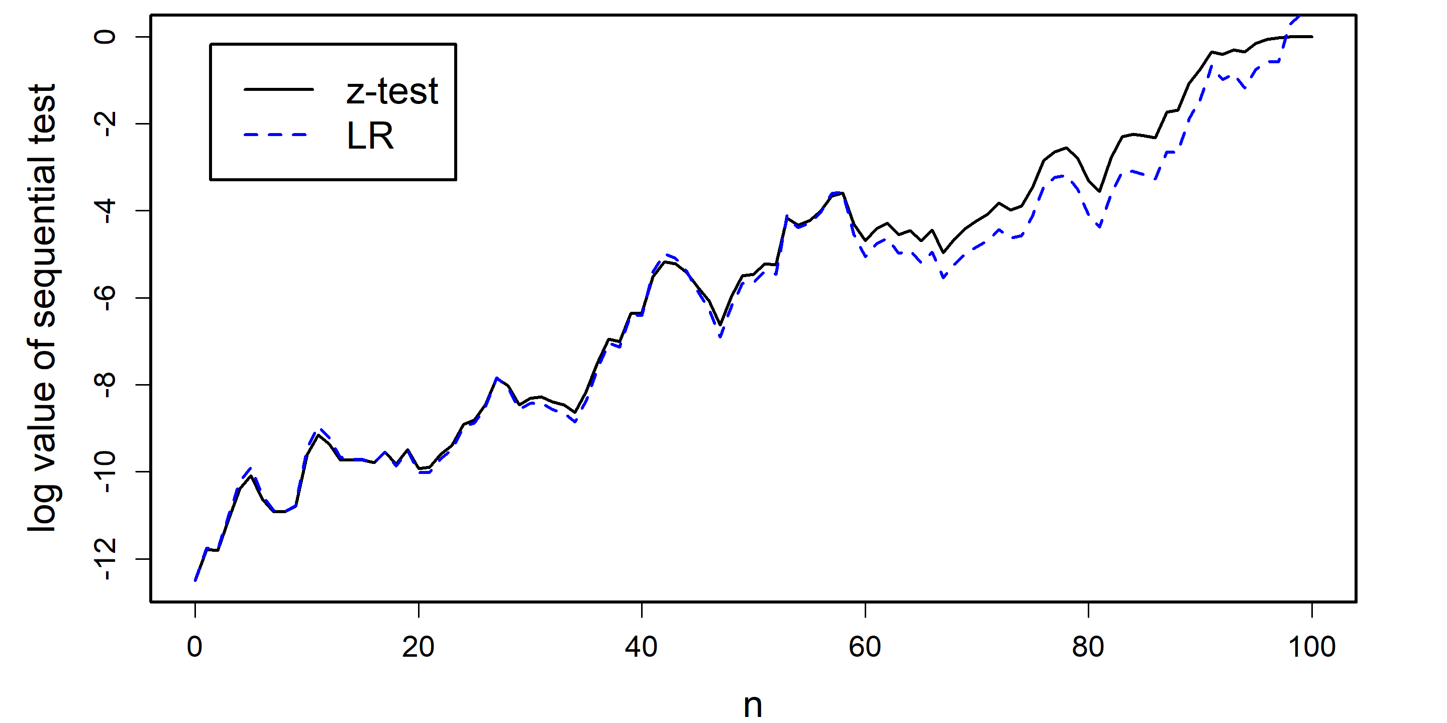
Figure 2: Illustration of the sequential $z$-test at $N=100$ and the likelihood ratio process over 100 observations sampled from $\mathcal{N}(0.5,1)$. The $z$-test is executed at significance level $\alpha=\exp\{-N\frac{\mu^{2}}{2\sigma^{2}}\}=\exp\{-12.5\}\approx.0000037$, for which Theorem 3 predicts that two sequential tests coincide as $N\to\infty$.

Remark 5 (Link to Breiman (1961)).

Our Theorem 3 is related to a result by Breiman (1961). In particular, he shows in a binary context that the power of the likelihood ratio process $(\alpha\text{LR}_{n}\wedge 1)_{n\in\mathbb{N}}$ at the final time $N$ asymptotically matches the power of the most powerful test at time $N$, uniformly in $\alpha$.

Our result shows something much stronger: for a particular choice of $\alpha$ the entire test processes themselves coincide as $N\to\infty$, not just their power at time $N$.

6 Acknowledgments

We sincerely thank Wouter Koolen for feedback on an early presentation of this work: he confirmed our suspicions that our results were far more general than we were able to show at the time. Moreover, we thank Aaditya Ramdas, Lasse Fischer and Simon Benhaiem for their comments.

Appendix A Proof of Theorem 3

Proof.

Under $\mathbb{P}$, the log-likelihood ratio is Gaussian

$$\log\textnormal{LR}_{N}\sim\mathcal{N}\left(-N\frac{\mu^{2}}{2\sigma^{2}},N\frac{\mu^{2}}{\sigma^{2}}\right).$$

The level $\alpha_{N}$ $z$-test can be written as a likelihood ratio test:

$$\phi_{N,\alpha_{N}}=\mathbb{I}\left[\log\textnormal{LR}_{N}>\frac{|\mu|}{\sigma}z_{1-\alpha_{N}}\sqrt{N}-N\frac{\mu^{2}}{2\sigma^{2}}\right].$$ (10)

To study its behavior as $\alpha_{N}\to 0$, we use the tail approximation of $z_{1-\alpha_{N}}$,

$$z_{1-\alpha_{N}} =\sqrt{-2\log\alpha_{N}}\left((1-\frac{\log(-\log(\alpha_{N}))+\log(4\pi)}{-4\log(\alpha_{N})}\right)$$

$$+\mathcal{O}\left(\frac{1}{({\log\alpha_{N}})^{3/2}}\right)$$

$$=\sqrt{N}\frac{|\mu|}{\sigma}-\frac{\log\left(\sqrt{2\pi\frac{N\mu^{2}}{\sigma^{2}}}\right)}{\sqrt{\frac{N\mu^{2}}{\sigma^{2}}}}+o\left(\frac{1}{\sqrt{N}}\right),$$

Plugging this approximation into (10) yields

$$\phi_{N,\alpha_{N}} =\mathbb{I}\left[\log\textnormal{LR}_{N}>N\frac{\mu^{2}}{2\sigma^{2}}-\underbrace{\log\left(\sqrt{\frac{2\pi N\mu^{2}}{\sigma^{2}}}\right)}_{c_{N}}+o(1)\right]$$ (11)

$$=\mathbb{I}\left[\log\textnormal{LR}_{N}>N\frac{\mu^{2}}{2\sigma^{2}}-c_{N}+o(1)\right].$$

Its conditional rejection probability can be rewritten as

$$\hskip-14.22636pt\phi^{\prime}_{n,\alpha_{N}} =\mathbb{E}^{\mathbb{P}}[\phi_{N,\alpha_{N}}\mid\textnormal{LR}_{n}]$$

$$=\mathbb{P}\left[\log\textnormal{LR}_{(N-n+1):N}>N\frac{\mu^{2}}{2\sigma^{2}}-\log\textnormal{LR}_{n}-c_{N}+o(1)\right]$$

$$=1-\Phi\left(\frac{N\frac{\mu^{2}}{2\sigma^{2}}-\log\textnormal{LR}_{n}-c_{N}+o(1)+\frac{(N-n)\mu^{2}}{2\sigma^{2}}}{\sqrt{(N-n)\frac{\mu^{2}}{\sigma^{2}}}{}}\right)$$

$$=1-\Phi\left(\frac{N\frac{\mu^{2}}{\sigma^{2}}-\log\textnormal{LR}_{n}-c_{N}+o(1)-n\frac{\mu^{2}}{2\sigma^{2}}}{\sqrt{(N-n)\frac{\mu^{2}}{\sigma^{2}}}}\right)$$ (12)

We use the approximation of the Gaussian survival function,

$$1-\Phi(z)=\frac{1}{z\sqrt{2\pi}}\exp\left\{\frac{-z^{2}}{2}\right\}+\mathcal{O}\left(\frac{1}{z^{3}}\exp\left\{\frac{-z^{2}}{2}\right\}\right).$$

To prepare for applying this approximation, we inspect $\frac{1}{z\sqrt{{2\pi}}}$, where $z$ corresponds to the argument in (12),

$$\frac{\sqrt{N-n}{\frac{|\mu|}{\sigma}}}{\sqrt{2\pi}\left(N\frac{\mu^{2}}{\sigma^{2}}-\log\textnormal{LR}_{n}-c_{N}+o(1)-n\frac{\mu^{2}}{2\sigma^{2}}\right)}=$$

$$=\frac{\sqrt{N}\frac{|\mu|}{\sigma}}{\sqrt{2\pi}N\frac{\mu^{2}}{\sigma^{2}}}+o(1)=\frac{1}{\sqrt{2\pi N\frac{\mu^{2}}{\sigma^{2}}}}+o(1)$$

$$=\exp\{-c_{N}\}+o(1),$$

where $c_{N}$ is the term defined in (11). Next, we consider the squared term in the Gaussian approximation,

$$\left(\frac{N\frac{\mu^{2}}{\sigma^{2}}-\log\textnormal{LR}_{n}-c_{N}+o(1)-n\frac{\mu^{2}}{2\sigma^{2}}}{\sqrt{N-n}{\frac{|\mu|}{\sigma}}}\right)^{2}=$$

$$=\frac{N^{2}\frac{\mu^{2}}{\sigma^{2}}-2N\left(\log\textnormal{LR}_{n}+c_{N}+n\frac{\mu^{2}}{2\sigma^{2}}\right)}{N-n}+o(1)$$

$$=N\frac{\mu^{2}}{\sigma^{2}}\frac{N-n}{N-n}-\frac{2N}{N-n}(\log\textnormal{LR}_{n}+c_{N})+o(1)$$

$$=-2\log(\alpha_{N})-2\frac{N}{N-n}(\log\textnormal{LR}_{n}+c_{N})+o(1).$$

Applying the approximation yields

$$\phi^{\prime}_{n,\alpha_{N}} =\exp\{-c_{N}\}\alpha_{N}\exp\left\{\frac{N(\log\textnormal{LR}_{n}+c_{N})}{N-n}\right\}+o(\alpha_{N}).$$

$$=\exp\left\{{\left(\frac{N}{N-n}-1\right)c_{N}}\right\}\alpha_{N}{LR}_{n}^{\frac{N}{N-n}}+o(\alpha_{N})$$

$$=\exp\left\{{o\left(\frac{1}{N}\right)o\left(\log(N)\right)}\right\}\alpha_{N}{LR}_{n}^{\frac{N}{N-n}}+o(\alpha_{N})$$

$$=\exp\left\{o(1)\right\}\alpha_{N}{LR}_{n}^{\frac{N}{N-n}}+o(\alpha_{N})$$

Hence,

$$\lim_{N\to\infty}\frac{\phi^{\prime}_{n,\alpha_{N}}}{\alpha_{N}}=\textnormal{LR}_{n}.$$

∎

References

- Breiman (1961) Leo Breiman. Optimal gambling systems for favorable games. The Kelly Capital Growth Investment Criterion, pages 47–60, 1961.
- Fischer and Ramdas (2024) Lasse Fischer and Aaditya Ramdas. Improving the (approximate) sequential probability ratio test by avoiding overshoot. arXiv preprint arXiv:2410.16076, 2024.
- Grünwald et al. (2023) Peter Grünwald, Rianne de Heide, and Wouter Koolen. Safe testing. arXiv preprint arXiv:1906.07801, 2023.
- Howard et al. (2020) Steven R Howard, Aaditya Ramdas, Jon McAuliffe, and Jasjeet Sekhon. Time-uniform chernoff bounds via nonnegative supermartingales. Probability Surveys, 17:257–317, 2020.
- Howard et al. (2021) Steven R. Howard, Aaditya Ramdas, Jon McAuliffe, and Jasjeet Sekhon. Time-uniform, nonparametric, nonasymptotic confidence sequences. The Annals of Statistics, 49(2):1055 – 1080, 2021. doi: 10.1214/20-AOS1991.
- Koning (2024a) Nick W. Koning. Continuous testing: Unifying tests and e-values, 2024a. URL https://arxiv.org/abs/2409.05654.
- Koning (2024b) Nick W. Koning. Post-hoc hypothesis testing and the post-hoc -value, 2024b. URL https://arxiv.org/abs/2312.08040.
- Lachin (2005) John M. Lachin. A review of methods for futility stopping based on conditional power. Statistics in Medicine, 24(18):2747–2764, 2005. doi: https://doi.org/10.1002/sim.2151.
- Lan et al. (1982) K.K. Gordon Lan, Richard Simon, and Max Halperin. Stochastically curtailed tests in long–term clinical trials. Communications in Statistics. Part C: Sequential Analysis, 1(3):207–219, 1982. doi: 10.1080/07474948208836014.
- Ramdas et al. (2022) Aaditya Ramdas, Johannes Ruf, Martin Larsson, and Wouter Koolen. Admissible anytime-valid sequential inference must rely on nonnegative martingales. arXiv preprint arXiv:2009.03167, 2022.
- Ramdas et al. (2023) Aaditya Ramdas, Peter Grünwald, Vladimir Vovk, and Glenn Shafer. Game-theoretic statistics and safe anytime-valid inference. Statistical Science, 38(4):576–601, 2023.
- Shafer (2021) Glenn Shafer. Testing by betting: A strategy for statistical and scientific communication. Journal of the Royal Statistical Society Series A: Statistics in Society, 184(2):407–431, 2021.
- Vovk and Wang (2021) Vladimir Vovk and Ruodu Wang. E-values: Calibration, combination and applications. The Annals of Statistics, 49(3):1736–1754, 2021.