Robust Moving-horizon Estimation for Nonlinear Systems: From Perfect to Imperfect Optimization

Abstract

Robust stability of moving-horizon estimators is investigated for nonlinear discrete-time systems that are detectable in the sense of incremental input/output-to-state stability and are affected by disturbances. The estimate of a moving-horizon estimator stems from the on-line solution of a least-squares minimization problem at each time instant. The resulting stability guarantees depend on the optimization tolerance in solving such minimization problems. Specifically, two main contributions are established: (i) the robust stability of the estimation error, while supposing to solve exactly the on-line minimization problem; (ii) the practical robust stability of the estimation error with state estimates obtained by an imperfect minimization. Finally, the construction of such robust moving-horizon estimators and the performances resulting from the design based on the theoretical findings are showcased with two numerical examples.

Keywords Robust moving-horizon estimation  $\cdot$ Incremental input/output-to-state stability  $\cdot$ Optimization  $\cdot$ Multiplicative noise

1 Introduction

We investigate the robust stability of the estimation error for moving-horizon estimators, which result from the exact on-line minimization of a least-squares cost function by using only a recent batch of information on the plant under monitoring. Specifically, we will show how to ensure robustness according to [1] by suitably discounting the effect of all the previous noises on the current state estimate, i.e., in other words, by properly choosing the cost function. Moreover, it will be shown that the estimation error is practically robustly stable with imperfect on-line optimization, namely by stopping the optimization if the norm of the gradient of the cost function is sufficiently small but not necessarily zero.

After the introduction of the input-to-state stability (ISS) in [2], output-to-state stability (OSS) is proposed by Sontag and Wang in [3] as extension of detectability to nonlinear systems without inputs. Incremental input/output-to-state stability (i-IOSS) is adopted in [3] to deal with inputs and outputs separately in general as well as it is shown that systems admitting robust estimators must be i-IOSS. Unfortunately, these results do not apply to moving-horizon estimators; only in [4, 5] the robust stability of moving-horizon estimation under the assumption of bounded disturbances was related to i-IOSS. Robust stability was proved without this boundedness assumption in [6], but under suitable conditions derived from the solution of the so-called full information estimation (FIE) problem. Other or slightly different conditions were considered in [7] and later in [8, 9, 10], and finally relaxed in [11] for incremental uniform exponential input/output-to-state stable (i-UEIOSS) systems.

The characterization of i-IOSS in terms of Lyapunov functions is addressed in [1] for discrete-time nonlinear systems under quite general assumptions and in line with previous results by Angeli (see [12, 13]) for continuous-time nonlinear systems. The findings of [1] on i-UIOSS (incremental uniform IOSS) and i-UEIOSS have provided the design of moving-horizon estimators for nonlinear discrete-time systems with a solid basis. First results based on this ground are presented in [14, 6, 8, 10], where the link between FIE and moving horizon estimation is investigated. All the approaches to moving-horizon estimation recalled so far demand the exact solution of the on-line minimization problems. In this paper, we present new results on moving-horizon estimation under imperfect optimization, i.e., we suppose to stop the minimization without exactly finding the minimizer of the cost in such a way as to reduce the computational burden. In this case, practical robust stability is proved to hold.

Reducing the on-line computational effort is a crucial issue in moving-horizon estimation [15, 16]. Among others, in [17, 18] moving-horizon estimation was addressed by using only few predetermined iterations of descent methods. Accelerated gradient-based approaches to moving-horizon estimation were investigated in [19, 20]. Compared to all the latter, here we rely on a relaxed stopping criterion, in that the descent algorithm is terminated if the gradient of the cost function is sufficiently small.

The paper is organized as follows. Section 2 is focused on moving horizon estimation with exact solution of the on-line minimization problem. In case of perfect optimization, we assume i-UIOSS, which is more general than i-UEIOSS. In Section 3, we deal with the robust stability properties of the considered moving-horizon estimators in case of imperfect optimization and assuming i-UEIOSS. Section 4 illustrates two case studies, while also including and discussing numerical results. Finally, conclusions are given in Section 5.

Given the vectors $\,v_{i},v_{i+1},\ldots,v_{j}$ for $i<j$, we define $\,v_{i}^{j}:=\left(v_{i},v_{i+1},\ldots,v_{j}\right)$. ${\mathop{\mathbb{R}}}_{\geq 0}$ and ${\mathop{\mathbb{N}}}_{\geq k}$ denote $[0,+\infty)$ and $\{k,k+1,\ldots\}$ with $k$ integer, respectively. A function $\alpha:{\mathop{\mathbb{R}}}_{\geq 0}\rightarrow{\mathop{\mathbb{R}}}_{\geq 0}$ is of class ${\mathcal{K}}$ if it is continuous, strictly increasing, and $\alpha(0)=0$. If in addition $\lim_{s\rightarrow\infty}\alpha(s)=+\infty$, it is of class ${\mathcal{K}}_{\infty}$. A function $\beta:{\mathop{\mathbb{R}}}_{\geq 0}\times{\mathop{\mathbb{N}}}_{\geq 0}\rightarrow{\mathop{\mathbb{R}}}_{\geq 0}$ is of class ${\mathcal{K}L}$ if $\beta(\cdot,k)$ is of class ${\mathcal{K}}$ for any fixed $k\in{\mathop{\mathbb{N}}}_{\geq 0}$ and $\beta(s,\cdot)$ is nonincreasing and $\lim_{k\rightarrow\infty}\beta(s,k)=0$ for any fixed $s\in{\mathop{\mathbb{R}}}_{\geq 0}$. Let us denote by $\oplus$ and $\wedge$ the maximum and minimum operators, i.e., $a\oplus b:=\max(a,b)$ and $a\wedge b:=\min(a,b)$ for any $a,b\in{\mathop{\mathbb{R}}}$, respectively. Moreover, for the sake of brevity let us define

$$\scalebox{1.5}{$\oplus$}_{i=1}^{n}a_{i}:=\max\left(a_{1},\ldots,a_{n}\right)$$

for any $n\in{\mathop{\mathbb{N}}}_{\geq 2}$. The $\oplus$ operator has higher precedence than the scalar product, i.e., $c\,a\oplus b=(ac)\oplus(bc)$ for any $a,b\in{\mathop{\mathbb{R}}}$ and $c\in{\mathop{\mathbb{R}}}_{\geq 0}$. For any column vector $x\in{\mathop{\mathbb{R}}}^{n}$, $|x|:=\sqrt{x^{\top}x}$ denotes the Euclidean norm; $x>0$ means that $x_{i}>0$, $i=1,\ldots,n$.

2 Moving-horizon Estimation with Perfect Optimization

In this section we will address moving-horizon estimation for discrete-time systems described by

$$\left\{\begin{array}[]{l}x_{t+1}=f(x_{t},w_{t})\\ y_{t}=h(x_{t},v_{t})\end{array}\,,\,t=0,1,\ldots\right.$$ (1)

where $x_{t}\in\mathbb{X}\subseteq{\mathop{\mathbb{R}}}^{n}$ is the state vector, $y_{t}\in{\mathop{\mathbb{R}}}^{m}$ is the measurement vector, $w_{t}\in\mathbb{W}\subseteq{\mathop{\mathbb{R}}}^{n}$ is the system noise, and $v_{t}\in\mathbb{V}\subseteq{\mathop{\mathbb{R}}}^{m}$ is the measurement noise. For such systems we assume that i-IOSS holds uniformly according to the following definition, where we denote by $x_{t}(\bar{x},\bar{w}_{0}^{t-1})$ the state of the system (1) at time $t=1,2,\ldots$ with initial state $\bar{x}\in\mathbb{X}$ in $t=0$ and system disturbances $\bar{w}_{0},\ldots,\bar{w}_{t-1}\in\mathbb{W}$.

Definition 1

System (1) is i-UIOSS (uniformly i-IOSS) if there exist ${\mathcal{K}L}$ functions $\beta_{x}(\cdot,\cdot),\beta_{w}(\cdot,\cdot)$, $\beta_{y}(\cdot,\cdot)$, $\beta_{v}(\cdot,\cdot)$ such that

$$\left|x_{t}(\bar{x},\bar{w}_{0}^{t-1})-x_{t}(\tilde{x},\tilde{w}_{0}^{t-1})\right|\leq\beta_{x}\left(\left|\bar{x}-\tilde{x}\right|,t\right)\oplus\scalebox{1.5}{$\oplus$}_{i=0}^{t-1}\beta_{w}\left(|\bar{w}_{i}-\tilde{w}_{i}|,t\!-\!1\!-\!i\right)$$

$$\oplus\scalebox{1.5}{$\oplus$}_{i=0}^{t-1}\beta_{y}\big{(}\big{|}h(x_{i}(\bar{x},\bar{w}_{0}^{i-1}),\bar{v}_{i})-h(x_{i}(\tilde{x},\tilde{w}_{0}^{i-1}),\tilde{v}_{i})\big{|},t\!-\!1\!-\!i\big{)}\oplus\scalebox{1.5}{$\oplus$}_{i=0}^{t-1}\beta_{v}\left(|\bar{v}_{i}-\tilde{v}_{i}|,t\!-\!1\!-\!i\right)\,,\,t=0,1,\ldots$$ (2)

for all $\bar{x},\tilde{x}\in\mathbb{X}$, $\bar{w}_{t},\tilde{w}_{t}\in\mathbb{W}$, $\bar{v}_{t},\tilde{v}_{t}\in\mathbb{V}$.

Definition 1 was proposed in [8, see Definition 1, p. 3]) and turns out to be quite general as compared to what is available in the literature since it allows to deal with multiplicative measurement noises, as it will be shown in Section 4.2.

Remark 1

In principle, there are no difficulties in developing what is presented in the following by using a system representation that includes some known input $u_{t}\in\mathbb{U}\subseteq{\mathop{\mathbb{R}}}^{p}$ in the system dynamics, i.e., using $x_{t+1}=f(x_{t},u_{t},w_{t})$ instead of $x_{t+1}=f(x_{t},w_{t})$. Unfortunately, this would complicate the notation, thus we prefer to treat the problems in a simpler form without $u_{t}$.

As shown in [1], it is necessary for a system to be i-IUOSS for admitting a robust estimator, where, as estimator, we mean a generic input/output mapping between the current available information up to $t$ and the estimate of $x_{t}$ denoted by $\hat{x}_{t|t}\in\mathbb{X}$, starting just with some “a priori” prediction of $x_{0}$ denoted by $\bar{x}_{0}\in\mathbb{X}$.

Definition 2

An estimator for system (1) with $\hat{x}_{t|t}\in\mathbb{X}$ as estimate of $x_{t}$ at time $t$ is robustly stable if there exist ${\mathcal{K}L}$ functions $\rho_{x}(\cdot,\cdot),\rho_{w}(\cdot,\cdot),\rho_{v}(\cdot,\cdot)$ such that

$$\left|x_{t}-\hat{x}_{t|t}\right|\leq\rho_{x}\left(\left|x_{0}-\bar{x}_{0}\right|,t\right)\oplus\scalebox{1.5}{$\oplus$}_{i=0}^{t-1}\rho_{w}\left(\left|w_{i}\right|,t\!-\!1\!-\!i\right)\oplus\scalebox{1.5}{$\oplus$}_{i=0}^{t-1}\rho_{v}\left(\left|v_{i}\right|,t\!-\!1\!-\!i\right)$$ (3)

for all $t=0,1,\ldots$.

Definition 1 is equivalent to detectability. For detectable linear discrete-time systems, it is easily shown the robust stability of the estimation error w.r.t noises by using summation instead of maximization in Definition 2 (see, e.g., [1, pp. 3020-3021]).

We consider the problem of estimating $x_{t}$ at time $t$ according to the moving-horizon paradigm, i.e., by using the batch of the last $t\wedge\!N$ measurements $y_{t-t\wedge\!N},\ldots,y_{t-1}$. At any $t$ we obtain the estimate $\hat{x}_{t|t}\in\mathbb{X}$ of $x_{t}$ by minimizing a cost function where the deviation from some “prediction” of the state $x_{t-t\wedge\!N}$ (denoted by $\bar{x}_{t-t\wedge N}$) and the fitting of $y_{t-t\wedge\!N},\ldots,y_{t-1}$ are penalized as follows

$$J_{t}^{t\wedge\!N}\left(\hat{x}_{t-t\wedge\!N},\hat{v}_{t-t\wedge\!N}^{t-1},\hat{w}_{t-t\wedge\!N}^{t-1}\right)=\beta_{x}(2\,|\hat{x}_{t-t\wedge\!N}-\bar{x}_{t-t\wedge\!N}|,{t\wedge\!N})\oplus\scalebox{1.5}{$\oplus$}_{i=t-t\wedge\!N}^{t-1}\,\beta_{w}\left(2\left|\hat{w}_{i}\right|,t\!-\!1\!-\!i\right)$$

$$\oplus\scalebox{1.5}{$\oplus$}_{i=t-t\wedge\!N}^{t-1}\,\beta_{y}\left(\left|y_{i}-h(\hat{x}_{i},\hat{v}_{i})\right|,t\!-\!1\!-\!i\right)\oplus\scalebox{1.5}{$\oplus$}_{i=t-t\wedge\!N}^{t-1}\,\beta_{v}\left(2\left|\hat{v}_{i}\right|,t\!-\!1\!-\!i\right)\,,\,t=1,2,\ldots$$ (4)

where $\beta_{x}(\cdot,\cdot),\beta_{w}(\cdot,\cdot),\beta_{y}(\cdot,\cdot),\beta_{v}(\cdot,\cdot)$ are the same ${\mathcal{K}L}$ functions involved in the definition of i-UIOSS for system (1) and the constraints

$$\hat{x}_{i+1}=f(\hat{x}_{i},\hat{w}_{i})\,,\,i=t-t\wedge\!N,\ldots,t-1$$

are implicitly considered in (4); moreover, we rely on the predictions given by

$$\bar{x}_{t-t\wedge N}=\left\{\begin{array}[]{ll}\bar{x}_{0}&t=1,\ldots,N\\ \hat{x}_{t-N|t-N}&t=N+1,N+2,\ldots\,.\end{array}\right.$$ (5)

Since the cost is continuous, minimizers of (4) exist under the usual assumptions required by the Weierstrass’ theorem, i.e., lower semicontinuity of the cost function and compactness or closeness of the domain (coercivity of the cost is required too in case closeness holds but compactness does not) [21, Proposition A.8, p. 669]. In this respect, $f(\cdot,\cdot)$ and $h(\cdot,\cdot)$ are assumed to be smooth enough as well.

We denote by MHE_N a generic moving-horizon estimator, which provides an estimate $\hat{x}_{t|t}$ of $x_{t}$ at time $t$ as the result of minimization of (4), together with (5). Thus, at each $t=1,2,\ldots$ we have to solve

$$\left(\hat{x}_{t-t\wedge N|t},\hat{v}_{t-t\wedge N|t}^{t-1},\hat{w}_{t-t\wedge N|t}^{t-1}\right) \in\displaystyle\!\!\!\!\mathop{{\rm argmin}}_{\begin{array}[]{c}\hat{x}_{t-t\wedge N}\in\mathbb{X},\hat{v}_{t-t\wedge N}^{t-1}\!\in\\ \mathbb{V}^{t\wedge N},\hat{w}_{t-t\wedge N}^{t-1}\in\mathbb{W}^{t\wedge N}\end{array}}\!\!\!\!\!\!J_{t}^{t\wedge\!N}\left(\hat{x}_{t-t\wedge N},\hat{v}_{t-t\wedge N}^{t-1},\hat{w}_{t-t\wedge N}^{t-1}\right)$$ (8)

and we get $\hat{x}_{t|t}$ by means of $\hat{x}_{i+1|t}=f(\hat{x}_{i|t},\hat{w}_{i|t})\,,\,i=t-t\wedge\!N,\ldots,t-1\,.$

Theorem 1

If system (1) is i-UIOSS and there exist ${\mathcal{K}L}$ functions $\alpha_{x}(\cdot,\cdot),\alpha_{v}(\cdot,\cdot)$, $\alpha_{w}(\cdot,\cdot)$ and $N\in{\mathop{\mathbb{N}}}_{\geq 1}$ such that

$$\beta_{x}\left(4\beta_{x}(2s,k),N\right)\leq\alpha_{x}(s,k+N)$$ (9a)

$$\beta_{x}\left(2\alpha_{x}(s,k),N\right)\leq\alpha_{x}(s,k+N)$$ (9b)

$$\beta_{x}\left(4\beta_{w}(2s,k),N\right)\leq\alpha_{w}(s,k+N)$$ (10a)

$$\beta_{x}\left(2\alpha_{w}(s,k),N\right)\leq\alpha_{w}(s,k+N)$$ (10b)

$$\beta_{x}\left(4\beta_{v}(2s,k),N\right)\leq\alpha_{v}(s,k+N)$$ (11a)

$$\beta_{x}\left(2\alpha_{v}(s,k),N\right)\leq\alpha_{v}(s,k+N)$$ (11b)

for all $(s,k)\in[0,+\infty)\times{\mathop{\mathbb{N}}}_{\geq 0}$, the MHE_N resulting from (8) is robustly stable.

Proof. From the definition of minimum of the cost function, i.e.,

$$J_{t}^{t\wedge\!N}\left(\hat{x}_{t-t\wedge\!N|t},\hat{v}_{t-t\wedge\!N|t}^{t-1},\hat{w}_{t-t\wedge\!N|t}^{t-1}\right)\leq J_{t}^{t\wedge\!N}\left(x_{t-t\wedge\!N},v_{t-t\wedge\!N}^{t-1},w_{t-t\wedge\!N}^{t-1}\right)\,,$$

for any $t=1,2,\ldots$ we obtain

$$\beta_{x}\left(2\left|\hat{x}_{t-t\wedge\!N|t}-\bar{x}_{t-t\wedge\!N}\right|,t\wedge\!N\right)\oplus\scalebox{1.5}{$\oplus$}_{i=t-t\wedge\!N}^{t-1}\beta_{y}\big{(}\big{|}y_{i}-h\left(\hat{x}_{i|t},\hat{v}_{i|t}\right)\big{|},t\!-\!1\!-\!i\big{)}\oplus\scalebox{1.5}{$\oplus$}_{i=t-t\wedge\!N}^{t-1}\hat{\beta}_{v}\left(2\left|\hat{v}_{i|t}\right|,t\!-\!1\!-\!i\right)$$

$$\oplus\scalebox{1.5}{$\oplus$}_{i=t-t\wedge\!N}^{t-1}\beta_{w}\left(2\left|\hat{w}_{i|t}\right|,t\!-\!1\!-\!i\right)$$

$$\leq\beta_{x}(2|x_{t-t\wedge\!N}-\bar{x}_{t-t\wedge\!N}|,t\wedge\!N)\oplus\scalebox{1.5}{$\oplus$}_{i=t-t\wedge\!N}^{t-1}\beta_{y}\big{(}\underbrace{\left|y_{i}-h(x_{i},v_{i})\right|}_{=0},t\!-\!1\!-\!i\big{)}\oplus\scalebox{1.5}{$\oplus$}_{i=t-t\wedge\!N}^{t-1}\beta_{v}\left(2\left|v_{i}\right|,t\!-\!1\!-\!i\right)$$

$$\oplus\scalebox{1.5}{$\oplus$}_{i=t-t\wedge\!N}^{t-1}\beta_{w}\left(2\left|w_{i}\right|,t\!-\!1\!-\!i\right)\,.$$ (12)

Let us focus on three types of inequality to manipulate inequality (12). From

$$\left|x_{t-t\wedge\!N}-\hat{x}_{t-t\wedge\!N|t}\right| \leq\left|x_{t-t\wedge\!N}-\bar{x}_{t-t\wedge\!N}\right|+\big{|}\hat{x}_{t-t\wedge\!N|t}-\bar{x}_{t-t\wedge\!N}\big{|}$$

by using $\rho(a+b)\leq\rho(2a)+\rho(2b),\forall a,b\in{\mathop{\mathbb{R}}}_{\geq 0}$ with $\rho(\cdot)$ being any ${\mathcal{K}}$ function [2, Equation (12), p. 438] it follows that

$$\beta_{x}\left(\left|x_{t-t\wedge\!N}-\hat{x}_{t-t\wedge\!N|t}\right|,t\wedge\!N\right)-\beta_{x}(2|x_{t-t\wedge\!N}-\bar{x}_{t-t\wedge\!N}|,t\wedge\!N)\leq\beta_{x}\left(2\left|\hat{x}_{t-t\wedge\!N|t}-\bar{x}_{t-t\wedge\!N}\right|,t\wedge\!N\right)\,.$$ (13)

Likewise, from $\left|v_{i}-\hat{v}_{i|t}\right|\leq|v_{i}|+\left|\hat{v}_{i|t}\right|$ and $\left|w_{i}-\hat{w}_{i|t}\right|\leq|w_{i}|+\left|\hat{w}_{i|t}\right|$ we obtain

$$\beta_{v}\left(\left|v_{i}-\hat{v}_{i|t}\right|,t-1-i\right)-\beta_{v}\left(2|v_{i}|,t-1-i\right)\leq\hat{\beta}_{v}\left(2\left|\hat{v}_{i|t}\right|,t-1-i\right)$$ (14)

$$\beta_{w}\left(\left|w_{i}-\hat{w}_{i|t}\right|,t-1-i\right)-\beta_{w}\left(2|w_{i}|,t-1-i\right)\leq\beta_{w}\left(2\left|\hat{w}_{i|t}\right|,t-1-i\right)$$ (15)

for $i\!=\!t\!-\!t\wedge\!N,\ldots,t\!-\!1$.

We will rely on (13), (14), and (15) to deal with (12). Specifically, by using the upper bound $a+a\oplus b\leq 2\,a\oplus b\,,\,\forall a,b\in{\mathop{\mathbb{R}}}$, and (13), from (12) it follows that

$$\beta_{x}\left(\left|x_{t-t\wedge\!N}-\hat{x}_{t-t\wedge\!N|t}\right|,t\wedge\!N\right)\leq 2\,\beta_{x}\big{(}2|x_{t-t\wedge\!N}-\bar{x}_{t-t\wedge\!N}|,t\wedge\!N\big{)}\oplus\scalebox{1.5}{$\oplus$}_{i=t-t\wedge\!N}^{t-1}\beta_{v}\left(2\left|v_{i}\right|,t\!-\!1\!-\!i\right)$$

$$\oplus\scalebox{1.5}{$\oplus$}_{i=t-t\wedge\!N}^{t-1}\beta_{w}\left(2\left|w_{i}\right|,t\!-\!1\!-\!i\right)\,.$$ (16)

Similar bounds are established from (12) by using (14), i.e.,

$$\beta_{v}\left(\left|v_{i}-\hat{v}_{i|t}\right|,t\wedge\!N\right)\leq 2\,\beta_{x}\big{(}2|x_{t-t\wedge\!N}-\bar{x}_{t-t\wedge\!N}|,N\big{)}\oplus\scalebox{1.5}{$\oplus$}_{i=t-t\wedge\!N}^{t-1}\beta_{v}\left(2\left|v_{i}\right|,t\!-\!1\!-\!i\right)$$

$$\oplus\scalebox{1.5}{$\oplus$}_{i=t-t\wedge\!N}^{t-1}\beta_{w}\left(2\left|w_{i}\right|,t\!-\!1\!-\!i\right)\,,\,i\!=\!t\!-\!t\wedge\!N,\ldots,t\!-\!1\,,$$ (17)

and (15), i.e.,

$$\beta_{w}\left(\left|w_{i}-\hat{w}_{i|t}\right|,t\wedge\!N\right)\leq 2\,\beta_{x}\big{(}|x_{t-t\wedge\!N}-\bar{x}_{t-t\wedge\!N}|,N\big{)}\oplus\scalebox{1.5}{$\oplus$}_{i=t-t\wedge\!N}^{t-1}\beta_{v}\left(2\left|v_{i}\right|,t\!-\!1\!-\!i\right)$$

$$\oplus\scalebox{1.5}{$\oplus$}_{i=t-t\wedge\!N}^{t-1}\beta_{w}\left(2\left|w_{i}\right|,t\!-\!1\!-\!i\right)\,,\,i\!=\!t\!-\!t\wedge\!N,\ldots,t-1.$$ (18)

Moreover, (12) yields

$$\!\!\!\!\scalebox{1.5}{$\oplus$}_{i=t-t\wedge\!N}^{t-1}\beta_{y}\big{(}\big{|}h(x_{i},v_{i})-h\left(\hat{x}_{i|t},\hat{v}_{i|t}\right)\big{|},t\!-\!1\!-\!i\big{)} \leq\beta_{x}\big{(}\big{|}x_{t-t\wedge\!N}-\bar{x}_{t-t\wedge\!N}\big{|},N\big{)}\oplus\scalebox{1.5}{$\oplus$}_{i=t-t\wedge\!N}^{t-1}\beta_{v}\left(2\left|v_{i}\right|,t\!-\!1\!-\!i\right)$$

$$\oplus\scalebox{1.5}{$\oplus$}_{i=t-t\wedge\!N}^{t-1}\beta_{w}\left(2\left|w_{i}\right|,t\!-\!1\!-\!i\right)$$

$$\leq 2\beta_{x}\big{(}2\big{|}x_{t-t\wedge\!N}-\bar{x}_{t-t\wedge\!N}\big{|},N\big{)}\oplus\scalebox{1.5}{$\oplus$}_{i=t-t\wedge\!N}^{t-1}\beta_{v}\left(2\left|v_{i}\right|,t\!-\!1\!-\!i\right)$$

$$\oplus\scalebox{1.5}{$\oplus$}_{i=t-t\wedge\!N}^{t-1}\beta_{w}\left(2\left|w_{i}\right|,t\!-\!1\!-\!i\right)\,,\,i\!=\!t\!-\!t\wedge\!N,\ldots,t-1.$$ (19)

Bringing (16)-(19) all together, we obtain

$$\beta_{x}\left(\left|x_{t-t\wedge\!N}-\hat{x}_{t-t\wedge\!N|t}\right|,t\wedge\!N\right)\oplus\scalebox{1.5}{$\oplus$}_{i=t-t\wedge\!N}^{t-1}\beta_{y}\big{(}\big{|}h(x_{i},v_{i})-h\left(\hat{x}_{i|t},\hat{v}_{i|t}\right)\big{|},t\!-\!1\!-\!i\big{)}$$

$$\oplus\scalebox{1.5}{$\oplus$}_{i=t-t\wedge\!N}^{t-1}\beta_{v}\left(\left|v_{i}-\hat{v}_{i|t}\right|,t\!-\!1\!-\!i\right)\oplus\scalebox{1.5}{$\oplus$}_{i=t-t\wedge\!N}^{t-1}\beta_{w}\left(\left|w_{i}-\hat{w}_{i|t}\right|,t\!-\!1\!-\!i\right)$$

$$\leq 2\,\beta_{x}\big{(}2\,|x_{t-t\wedge\!N}-\bar{x}_{t-t\wedge\!N}|,N\big{)}\oplus\scalebox{1.5}{$\oplus$}_{i=t-t\wedge\!N}^{t-1}\beta_{v}\left(2\left|v_{i}\right|,t\!-\!1\!-\!i\right)\oplus\scalebox{1.5}{$\oplus$}_{i=t-t\wedge\!N}^{t-1}\beta_{w}\left(2\left|w_{i}\right|,t\!-\!1\!-\!i\right)$$

and thus

$$\left|x_{t}-\hat{x}_{t|t}\right|\leq 2\,\beta_{x}\big{(}2\,|x_{t-t\wedge\!N}-\bar{x}_{t-t\wedge\!N}|,t\wedge\!N\big{)}\oplus\scalebox{1.5}{$\oplus$}_{i=t-t\wedge\!N}^{t-1}\beta_{v}\left(2\left|v_{i}\right|,t\!-\!1\!-\!i\right)$$

$$\oplus\scalebox{1.5}{$\oplus$}_{i=t-t\wedge\!N}^{t-1}\beta_{w}\left(2\left|w_{i}\right|,t\!-\!1\!-\!i\right)\,,\,t=1,2,\ldots\,,$$ (20)

since system (1) is assumed to be i-UIOSS.

In the following, first of all we analyze the bounds derived from (20) when (i) $t=1,\ldots,N$, (ii) $t=N+1,\ldots,2N$, and (iii) $t\geq 2N+1$. Later, we will combine the previous results to prove robust stability in the sense of Definition 2.

Concerning (i), from (20) it is straightforward to get

$$\left|x_{t}-\hat{x}_{t|t}\right|\leq 2\,\beta_{x}\big{(}2|x_{0}-\bar{x}_{0}|,t\big{)}\oplus\scalebox{1.5}{$\oplus$}_{i=0}^{t-1}\beta_{v}\left(2\left|v_{i}\right|,t\!-\!1\!-\!i\right)\oplus\scalebox{1.5}{$\oplus$}_{i=0}^{t-1}\beta_{w}\left(2\left|w_{i}\right|,t\!-\!1\!-\!i\right)\,,\,t=1,\ldots,N\,.$$ (21)

Let us consider (ii). From (20) for $t=N+1$ we obtain

$$\left|x_{N+1}-\hat{x}_{N+1|N+1}\right|\leq 2\,\beta_{x}\big{(}2\,|x_{1}-\hat{x}_{1|1}|,N\big{)}\oplus\scalebox{1.5}{$\oplus$}_{i=1}^{N}\beta_{v}\left(2\left|v_{i}\right|,N\!-\!i\right)\oplus\scalebox{1.5}{$\oplus$}_{i=1}^{N}\beta_{w}\left(2\left|w_{i}\right|,N\!-\!i\right)$$ (22)

since $\bar{x}_{1}=\hat{x}_{1|1}$ and, using (21) for $t=1$, it follows that

$$\left|x_{N+1}-\hat{x}_{N+1|N+1}\right| \leq 2\,\beta_{x}\big{(}4\beta_{x}\big{(}2|x_{0}-\bar{x}_{0}|,1\big{)}\oplus\beta_{v}(2|v_{0}|,0)\oplus\beta_{w}(2|w_{0}|,0),N\big{)}\oplus\scalebox{1.5}{$\oplus$}_{i=1}^{N}\beta_{v}\left(\left|v_{i}\right|,N\!-\!i\right)$$

$$\oplus\scalebox{1.5}{$\oplus$}_{i=1}^{N}\beta_{w}\left(\left|w_{i}\right|,N\!-\!i\right)$$

$$=2\,\beta_{x}\big{(}4\beta_{x}\big{(}2|x_{0}-\bar{x}_{0}|,1\big{)},N\big{)}\oplus\beta_{x}\big{(}\beta_{v}(2|v_{0}|,0),N\big{)}\oplus\beta_{x}\big{(}\beta_{w}(2|w_{0}|,0),N\big{)}$$

$$\oplus\scalebox{1.5}{$\oplus$}_{i=1}^{N}\beta_{v}\left(2\left|v_{i}\right|,N\!-\!i\right)\oplus\scalebox{1.5}{$\oplus$}_{i=1}^{N}\beta_{w}\left(2\left|w_{i}\right|,N\!-\!i\right)$$

$$\leq 2\,\alpha_{x}\big{(}|x_{0}-\bar{x}_{0}|,N+1\big{)}\oplus\alpha_{v}(|v_{0}|,N)\oplus\scalebox{1.5}{$\oplus$}_{i=1}^{N}\beta_{v}\left(2\left|v_{i}\right|,N\!-\!i\right)\oplus\alpha_{w}(|w_{0}|,N)$$

$$\oplus\scalebox{1.5}{$\oplus$}_{i=1}^{N}\beta_{w}\left(2\left|w_{i}\right|,N\!-\!i\right)$$ (23)

by using (9a), (11a), and (10a). Proceeding similarly for $t=N+2,\ldots,2N$, we get

$$\left|x_{t}-\hat{x}_{t|t}\right| \leq 2\,\alpha_{x}\big{(}2|x_{0}-\bar{x}_{0}|,t\big{)}\oplus\scalebox{1.5}{$\oplus$}_{i=0}^{t-N-1}\alpha_{v}\left(\left|v_{i}\right|,t\!-\!1\!-\!i\right)\oplus\scalebox{1.5}{$\oplus$}_{i=t-N}^{t-1}\beta_{v}\left(2\left|v_{i}\right|,t\!-\!1\!-\!i\right)$$

$$\oplus\scalebox{1.5}{$\oplus$}_{i=0}^{t-N-1}\alpha_{w}\left(\left|w_{i}\right|,t\!-\!1\!-\!i\right)\oplus\scalebox{1.5}{$\oplus$}_{i=t-N}^{t-1}\beta_{w}\left(2\left|w_{i}\right|,t\!-\!1\!-\!i\right)\,,\,t=N+1,\ldots,2N\,.$$ (24)

In case of (iii), for $t=2N+1$ we need to use both (20) and (24). It follows that

$$\left|x_{2N+1}-\hat{x}_{2N+1|2N+1}\right| \leq 2\,\beta_{x}\big{(}2\,|x_{N+1}-\hat{x}_{N+1|N+1}|,N\big{)}\oplus\scalebox{1.5}{$\oplus$}_{i=N+1}^{2N}\beta_{v}\left(2\left|v_{i}\right|,2N\!-\!i\right)$$

$$\oplus\scalebox{1.5}{$\oplus$}_{i=N+1}^{2N}\beta_{w}\left(2\left|w_{i}\right|,2N\!-\!i\right)$$

and thus by using (23)

$$\left|x_{2N+1}-\hat{x}_{2N+1|2N+1}\right| \leq 2\,\beta_{x}\Big{(}2\,\alpha_{x}\big{(}|x_{0}-\bar{x}_{0}|,N+1\big{)}\oplus\alpha_{v}(|v_{0}|,N)\oplus\scalebox{1.5}{$\oplus$}_{i=1}^{N}\beta_{v}\left(2\left|v_{i}\right|,N\!-\!i\right)\oplus\alpha_{w}(|w_{0}|,N)$$

$$\oplus\scalebox{1.5}{$\oplus$}_{i=1}^{N}\beta_{w}\left(2\left|w_{i}\right|,N\!-\!i\right),N\Big{)}\oplus\scalebox{1.5}{$\oplus$}_{i=N+1}^{2N}\beta_{v}\left(2\left|v_{i}\right|,2N\!-\!i\right)$$

$$\oplus\scalebox{1.5}{$\oplus$}_{i=N+1}^{2N}\beta_{w}\left(2\left|w_{i}\right|,2N\!-\!i\right)$$

$$\leq 2\,\beta_{x}\Big{(}2\,\alpha_{x}\big{(}|x_{0}-\bar{x}_{0}|,N+1\big{)},N\Big{)}\oplus\beta_{x}\Big{(}2\,\alpha_{v}(|v_{0}|,N),N\Big{)}\oplus\beta_{x}\Big{(}2\,\alpha_{w}(|w_{0}|,N),N\Big{)}$$

$$\oplus\scalebox{1.5}{$\oplus$}_{i=1}^{N}\beta_{x}\Big{(}\beta_{v}\left(2\left|v_{i}\right|,N\!-\!i\right),N\Big{)}\oplus\scalebox{1.5}{$\oplus$}_{i=1}^{N}\beta_{x}\Big{(}\beta_{w}\left(2\left|w_{i}\right|,N\!-\!i\right),N\Big{)}$$

$$\oplus\scalebox{1.5}{$\oplus$}_{i=N+1}^{2N}\beta_{v}\left(2\left|v_{i}\right|,2N\!-\!i\right)\oplus\scalebox{1.5}{$\oplus$}_{i=N+1}^{2N}\beta_{w}\left(2\left|w_{i}\right|,2N\!-\!i\right)\,.$$ (25)

Since (9b), (11b), and (10b) yield $\beta_{x}\Big{(}2\,\alpha_{x}\big{(}|x_{0}-\bar{x}_{0}|,N+1\big{)},N\Big{)}\leq\alpha_{x}\big{(}|x_{0}-\bar{x}_{0}|,2N+1\big{)}$, $\beta_{x}\Big{(}2\,\alpha_{v}(|v_{0}|,N),N\Big{)}\leq\alpha_{v}(|v_{0}|,2N)$, and $\beta_{x}\Big{(}2\,\alpha_{w}(|w_{0}|,N),N\Big{)}\leq\alpha_{w}(|w_{0}|,2N)$, respectively, as well as

$$\beta_{x}\Big{(}\beta_{w}\left(2|w_{i}|,N\!-\!i\right),N\Big{)}\leq\beta_{x}\Big{(}4\beta_{w}\left(2|w_{i}|,N\!-\!i\right),N\Big{)}\leq\alpha_{w}\left(|w_{i}|,2N\!-\!i\right)$$

$$\beta_{x}\Big{(}\beta_{v}\left(2\left|v_{i}\right|,N\!-\!i\right),N\Big{)}\leq\beta_{x}\Big{(}4\beta_{v}\left(2\left|v_{i}\right|,N\!-\!i\right),N\Big{)}\leq\alpha_{v}\left(|v_{i}|,2N\!-\!i\right)$$

by using (10a) and (11a), respectively, from (25) it follows that

$$\left|x_{2N+1}-\hat{x}_{2N+1|2N+1}\right| \leq 2\,\alpha_{x}\big{(}|x_{0}-\bar{x}_{0}|,2N+1\big{)}\oplus\scalebox{1.5}{$\oplus$}_{i=0}^{N}\alpha_{v}(|v_{i}|,2N\!-\!i)\oplus\scalebox{1.5}{$\oplus$}_{i=N+1}^{2N}\beta_{v}(2|v_{i}|,2N\!-\!i)$$

$$\oplus\scalebox{1.5}{$\oplus$}_{i=0}^{N}\alpha_{w}(|w_{i}|,2N\!-\!i)\oplus\scalebox{1.5}{$\oplus$}_{i=N+1}^{2N}\beta_{w}(2|w_{i}|,2N\!-\!i)\,,$$

which coincides with (24) for $t=2N+1$. In so doing for any $t\geq 2N+2$, we get that (24) holds for all $t\geq N+1$. Therefore, from combining (21) and (24) (holding for all $t\geq N+1$) robust stability is established for estimator MHE_N in the sense of Definition 2 by taking $\rho_{x}(s,t):=2\,\beta_{x}(2s,t)\oplus\alpha_{x}(s,t),\rho_{v}(s,t):=2\,\beta_{v}(2s,t)\oplus\alpha_{v}(s,t),\rho_{w}(s,t):=2\,\beta_{w}(2s,t)\oplus\alpha_{w}(s,t)$. $\Box$

Remark 2

Theorem 1 guarantees robust stability if the minimization problem is solved exactly, which corresponds to the choice of $A=1$ in [8, formulas (11), p. 4 and (22), p. 5]. Indeed, the satisfaction of [8, (11), p. 4] is nontrivial if $A>1$, which entails some suboptimality margin but, to be applied, demands the knowledge of the true state and disturbances. Moreover, in [8, 10] additional conditions concerning the FIE problem are required such as [8, (23)-(25) and Theorem 14, p. 6] and [10, Assumption 2, p. 4 and Assumption 3, p. 6]. By contrast, conditions (9a)-(11b) in Theorem 1 are simple and can be rigorously checked, as shown in the case study of Section 4.1.

Theorems 1 demands to minimize the cost function perfectly. In order to overcome this limitation, we will address moving-horizon estimation for a class of systems with additive disturbances and a quadratic cost function with exponential discount. More specifically, consider

$$\left\{\begin{array}[]{l}x_{t+1}=f(x_{t})+w_{t}\\ y_{t}=h(x_{t})+v_{t}\end{array}\,,\,t=0,1,\ldots\right.$$ (26)

and assume that incremental uniform exponential input/output-to-state stability (i-UEIOSS) holds for system (26) according to the following definition.

Definition 3

System (26) is i-UEIOSS if there exist $\eta\in(0,1)$ and $c_{x},c_{v},c_{w}>0$

$$\left|x_{t}(\bar{x},\bar{w}_{0}^{t-1})-x_{t}(\tilde{x},\tilde{w}_{0}^{t-1})\right|^{2} \leq c_{x}\left|\bar{x}-\tilde{x}\right|^{2}\eta^{t}+c_{v}\!\sum_{i=0}^{t-1}\!\eta^{t-1-i}\!\left|h(x_{i}(\bar{x},\bar{w}_{0}^{i-1}))\!+\!\bar{v}_{i}\!-\!h(x_{i}(\tilde{x},\tilde{w}_{0}^{i-1}))\!-\!\tilde{v}_{i}\right|^{2}$$

$$+c_{w}\!\sum_{i=0}^{t-1}\!\eta^{t-1-i}|\bar{w}_{i}-\tilde{w}_{i}|^{2}\,,\,t=1,2,\ldots$$ (27)

for all $\bar{x},\tilde{x}\in\mathbb{X}$, $\bar{v}_{t},\tilde{v}_{t}\in\mathbb{V}$, and $\bar{w}_{t},\tilde{w}_{t}\in\mathbb{W}$.

Definition 4

An estimator for system (26) with $\hat{x}_{t|t}$ as estimate of $x_{t}$ at time $t$ is exponentially robustly stable if

$$\left|x_{t}-\hat{x}_{t|t}\right|^{2} \leq\alpha\left|x_{0}-\bar{x}_{0}\right|^{2}\lambda^{t}+\beta\sum_{i=0}^{t-1}\lambda^{t-1-i}|v_{i}|^{2}+\gamma\sum_{i=0}^{t-1}\lambda^{t-1-i}|w_{i}|^{2}\,,\,t=1,2,\ldots$$ (28)

for some $\lambda\in(0,1)$, where $\alpha,\beta,\gamma>0$, and $\varepsilon$-practically exponentially robustly stable for some $\varepsilon>0$ if

$$\left|x_{t}-\hat{x}_{t|t}\right|^{2} \leq\alpha\left|x_{0}-\bar{x}_{0}\right|^{2}\lambda^{t}+\beta\sum_{i=0}^{t-1}\lambda^{t-1-i}|v_{i}|^{2}+\gamma\sum_{i=0}^{t-1}\lambda^{t-1-i}|w_{i}|^{2}+\varepsilon^{2}\,,\,t=1,2,\ldots$$ (29)

where again $\alpha,\beta,\gamma>0$ and $\lambda\in(0,1)$.

Definitions 3 and 4 are formulated by using squares of norm instead of norms since they are equivalent as $\sqrt{a+b}\leq\sqrt{a}+\sqrt{b}$, for all $a,b\geq 0$. This allows for some simplification without loss of generality when manipulating the inequalities necessary to prove the next findings.

From now on we suppose to know the i-UEIOSS discount factor $\eta\in(0,1)$ or at least some upper bound of $\eta$ just strictly less than one. Therefore, we consider the MHE_N providing the estimate $\hat{x}_{t|t}\in\mathbb{X}$ of $x_{t}$, obtained by minimizing the quadratic cost

$$J_{t}^{t\wedge\!N}\left(\hat{x}_{t-t\wedge\!N},\hat{w}_{t-t\wedge\!N}^{t-1}\right)=\mu\,\left|\hat{x}_{t-t\wedge\!N}-\bar{x}_{t-t\wedge\!N}\right|^{2}\eta^{t\wedge\!N}+\nu\!\!\sum_{i=t-{t\wedge\!N}}^{t-1}\eta^{t-1-i}\left|y_{i}-h(\hat{x}_{i})\right|^{2}+\omega\!\!\sum_{i=t-{t\wedge\!N}}^{t-1}\eta^{t-1-i}\left|\hat{w}_{i}\right|^{2}$$ (30)

at each time $t=1,2,\ldots$, where $\mu,\nu,\omega>0$, with implicit constraints

$$\hat{x}_{i+1}=f(\hat{x}_{i})+\hat{w}_{i}\,,\,i=t\!-\!t\wedge\!N,\ldots,t-1\,,$$

and predictions given by (5). Based on the aforesaid, we get the following theorem, which “mutatis mutandi” can be easily derived from [11, Proposition 1 and Theorem 1, p. 7469].

Theorem 2

If system (26) is i-UEIOSS and (30) is chosen with $\mu\geq c_{x}$, $\nu\geq c_{v}/2$, $\omega\geq c_{w}$, and $N\geq 1$ integer such that $4\,\mu\,\eta^{N}<1$, the MHE_N resulting from minimizing (30) is exponentially robustly stable in that, for each $t=1,2,\ldots$, there exists $\lambda\in(0,1)$ such that

$$\left|x_{t}-\hat{x}_{t|t}\right|^{2}\leq 4\,\mu|x_{0}-\bar{x}_{0}|^{2}\lambda^{t}+2\,\nu\sum_{i=0}^{t-1}\lambda^{t-1-i}|v_{i}|^{2}+4\,\omega\sum_{i=0}^{t-1}\lambda^{t-1-i}|w_{i}|^{2}$$ (31)

where $\hat{x}_{t|t}$ is the estimate of $x_{t}$. $\Box$

Proof. We split the proof into two cases.

First, let us focus on the cases $t=1,\ldots,N-1$. For $t=1$, the minimizer $\left(\hat{x}_{0|1},\hat{w}_{0|1}\right)$ provides the estimate $\hat{x}_{1|1}=f\left(\hat{x}_{0|1}\right)+\hat{w}_{0|1}$ and hence, by definition, we have $J_{1}^{1}\left(\hat{x}_{0|1},\hat{w}_{0|1}\right)\leq J_{1}^{1}\left(x_{0},w_{0}\right)$, i.e.,

$$\mu\left|\hat{x}_{0|1}-\bar{x}_{0}\right|^{2}\eta+\nu\left|y_{0}-h(\hat{x}_{0|1})\right|^{2}+\omega\left|\hat{w}_{0|1}\right|^{2}\leq\mu\left|x_{0}-\bar{x}_{0}\right|^{2}\eta+\nu\left|y_{0}-h(x_{0})\right|^{2}+\omega\left|w_{0}\right|^{2}\,.$$ (32)

Using the square sum bound, from $\left|x_{0}-\hat{x}_{0|1}\right|\leq\left|x_{0}-\bar{x}_{0}\right|+\left|\bar{x}_{0}-\hat{x}_{0|1}\right|$ it follows that

$$\left|x_{0}-\hat{x}_{0|1}\right|^{2}\leq 2\left|x_{0}-\bar{x}_{0}\right|^{2}+2\left|\bar{x}_{0}-\hat{x}_{0|1}\right|^{2}$$

and hence

$$\frac{1}{2}\left|x_{0}-\hat{x}_{0|1}\right|^{2}-\left|x_{0}-\bar{x}_{0}\right|^{2}\leq\left|\bar{x}_{0}-\hat{x}_{0|1}\right|^{2}$$ (33)

and in a similar way

$$\frac{1}{2}\left|w_{0}-\hat{w}_{0|1}\right|^{2}-\left|w_{0}\right|^{2}\leq\left|\hat{w}_{0|1}\right|^{2}\,.$$ (34)

Using (33) and (34), (32) yields

$$\mu\left|x_{0}-\hat{x}_{0|1}\right|^{2}\eta+2\,\nu\left|y_{0}-h(\hat{x}_{0|1})\right|^{2}+\omega\left|w_{0}-\hat{w}_{0|1}\right|^{2}\leq 4\,\mu\left|x_{0}-\bar{x}_{0}\right|^{2}+2\,\nu\left|v_{0}\right|^{2}+4\,\omega\left|w_{0}\right|^{2}$$

and hence

$$c_{x}\left|x_{0}-\hat{x}_{0|1}\right|^{2}\eta+c_{v}\left|h(x_{0})+v_{0}-h(\hat{x}_{0|1})\right|^{2}+c_{w}\big{|}w_{0}-\hat{w}_{0|1}\big{|}^{2}\leq 4\,\mu\left|x_{0}-\bar{x}_{0}\right|^{2}+2\,\nu\left|v_{0}\right|^{2}+4\,\omega\left|w_{0}\right|^{2}$$ (35)

because of the assumptions on $\mu$, $\nu$, and $\omega$. Thus, by using the i-UEIOSS assumption, from (35) it follows that

$$\left|x_{1}-\hat{x}_{1|1}\right|^{2}\leq 4\,\mu\left|x_{0}-\bar{x}_{0}\right|^{2}\eta+2\,\nu|v_{0}|^{2}+4\,\omega|w_{0}|^{2}\,,$$ (36)

namely (31) for $t=1$ with $\lambda=\eta$. We can proceed similarly for $t=2,\ldots,N-1$. Thus, we obtain

$$\left|x_{t}-\hat{x}_{t|t}\right|^{2}\leq 4\,\mu|x_{0}-\bar{x}_{0}|^{2}\eta^{t}+2\,\nu\sum_{i=0}^{t-1}\eta^{t-1-i}|v_{i}|^{2}+4\,\omega\sum_{i=0}^{t-1}\eta^{t-1-i}|w_{i}|^{2}\,,\,t=1,\ldots,N-1\,.$$ (37)

Second, from now on we focus on the cases $t=N,N+1,\ldots$. From the definition of minimum it follows that $J_{t}^{N}(\hat{x}_{t-N|t},\hat{w}_{t-N|t}^{t-1})\leq J_{t}^{N}(x_{t-N},w_{t-N}^{t-1})$, namely

$$\mu\,\left|\hat{x}_{t-N|t}-\bar{x}_{t-N}\right|^{2}\eta^{N}+\nu\sum_{i=t-N}^{t-1}\eta^{t-1-i}\left|y_{i}-h(\hat{x}_{i|t})\right|^{2}+\omega\sum_{i=t-N}^{t-1}\eta^{t-1-i}\left|\hat{w}_{i|t}\right|^{2}\leq\mu\,\left|x_{t-N}-\bar{x}_{t-N}\right|^{2}\eta^{N}$$

$$+\nu\sum_{i=t-N}^{t-1}\eta^{t-1-i}|v_{i}|^{2}+\omega\sum_{i=t-N}^{t-1}\eta^{t-1-i}|w_{i}|^{2}$$ (38)

for $t=N,N+1,\ldots$. Using the inequalities

$$\frac{1}{2}\left|x_{t-N}-\hat{x}_{t-N|t}\right|^{2}\!-\left|x_{t-N}-\bar{x}_{t-N}\right|^{2}\!\leq\!\left|\hat{x}_{t-N|t}-\bar{x}_{t-N}\right|^{2}\,,$$

$$\left|w_{i}-\hat{w}_{i|t}\right|^{2}/2-\left|w_{i}\right|^{2}\leq\left|\hat{w}_{i|t}\right|^{2}\,,\,i=t-N,\ldots,t-1\,,$$

(38) yields

$$\frac{\mu}{2}\,\left|x_{t-N}-\hat{x}_{t-N|t}\right|^{2}\eta^{N}+\nu\sum_{i=t-N}^{t-1}\eta^{t-1-i}\left|y_{i}-h(\hat{x}_{i|t})\right|^{2}+\frac{\omega}{2}\sum_{i=t-N}^{t-1}\eta^{t-1-i}\left|w_{i}-\hat{w}_{i|t}\right|^{2}\leq 2\mu\,\left|x_{t-N}-\bar{x}_{t-N}\right|^{2}\eta^{N}$$

$$+\nu\sum_{i=t-N}^{t-1}\eta^{t-1-i}|v_{i}|^{2}+2\,\omega\sum_{i=t-N}^{t-1}\eta^{t-1-i}|w_{i}|^{2}\,.$$

Since $\mu\geq c_{x}$, $\nu\geq c_{v}/2$, $\omega\geq c_{w}$ and the system is i-UEIOSS by assumption, we obtain

$$\left|x_{t}-\hat{x}_{t|t}\right|^{2}\leq 4\,\mu\left|x_{t-N}-\bar{x}_{t-N}\right|^{2}\eta^{N}+2\,\nu\sum_{i=t-N}^{t-1}\eta^{t-1-i}|v_{i}|^{2}+4\,\omega\sum_{i=t-N}^{t-1}\eta^{t-1-i}|w_{i}|^{2}$$ (39)

for all $t=N,N+1,\ldots$. In particular, from (39) it follows that

$$\left|x_{N}-\hat{x}_{N|N}\right|^{2}\leq 4\,\mu\left|x_{0}-\bar{x}_{0}\right|^{2}\eta^{N}+2\,\nu\sum_{i=0}^{N-1}\eta^{N-1-i}|v_{i}|^{2}+4\,\omega\sum_{i=0}^{N-1}\eta^{N-1-i}|w_{i}|^{2}$$ (40)

for $t=N$ and

$$\left|x_{N+1}-\hat{x}_{N+1|N+1}\right|^{2}\leq 4\,\mu\left|x_{1}-\hat{x}_{1|1}\right|^{2}\eta^{N}+2\,\nu\sum_{i=1}^{N}\eta^{N-i}|v_{i}|^{2}+4\,\omega\sum_{i=1}^{N}\eta^{N-i}|w_{i}|^{2}$$ (41)

for $t=N+1$. Using (36), from (41) we obtain

$$\left|x_{N+1}-\hat{x}_{N+1|N+1}\right|^{2} \leq 4\,\mu\,\left(4\,\mu\,\eta^{N+1}\right)\left|x_{0}-\bar{x}_{0}\right|^{2}+2\,\nu\left(4\,\mu\,\eta^{N}\left|v_{0}\right|^{2}+\sum_{i=1}^{N}\eta^{N-i}|v_{i}|^{2}\right)$$

$$+4\,\omega\left(4\,\mu\,\eta^{N}\left|w_{0}\right|^{2}+\sum_{i=1}^{N}\eta^{N-i}|w_{i}|^{2}\right)\,.$$ (42)

Based on the assumption $4\,\mu\,\eta^{N}<1$, for the theorem of sign permanence there exists $\alpha\in(0,1)$ such that $4\,\mu\,\eta^{\alpha N}<1$. Moreover, $\eta<\eta^{\alpha}<1$ and $\eta<\eta^{1-\alpha}<1$. Thus, we get

$$4\,\mu\,\eta^{N}=\underbrace{4\,\mu\,\eta^{\alpha N}}_{<1}\,\eta^{(1-\alpha)N}<\left(\eta^{1-\alpha}\right)^{N}$$

and

$$4\,\mu\,\eta^{N+1}=\underbrace{4\,\mu\,\eta^{\alpha(N+1)}}_{<1}\,\eta^{(1-\alpha)(N+1)}<\left(\eta^{1-\alpha}\right)^{N+1}\,.$$

Using such inequalities, from (42) it follows that

$$\left|x_{N+1}-\hat{x}_{N+1|N+1}\right|^{2}\leq 4\,\mu\,\left|x_{0}-\bar{x}_{0}\right|^{2}\left(\eta^{1-\alpha}\right)^{N+1}+2\,\nu\sum_{i=0}^{N}\left(\eta^{1-\alpha}\right)^{N-i}|v_{i}|^{2}+4\,\omega\sum_{i=0}^{N}\left(\eta^{1-\alpha}\right)^{N-i}|w_{i}|^{2}$$ (43)

and thus (31) holds for $t=N+1$ with $\lambda=\eta^{1-\alpha}$. Moreover, it is straightforward to turn (37) and (40) into (31) for $t=1,\ldots,N$ with $\lambda=\eta^{1-\alpha}$ by using the previous bounds. We can go on in a similar way up to $t=2N-1$. In more detail, let us consider (39) for $t=2N$, i.e.,

$$\left|x_{2N}-\hat{x}_{2N|2N}\right|^{2}\leq 4\,\mu\left|x_{N}-\hat{x}_{N|N}\right|^{2}\eta^{N}+2\,\nu\sum_{i=N}^{2N-1}\eta^{2N-1-i}|v_{i}|^{2}+4\,\omega\sum_{i=N}^{2N-1}\eta^{2N-1-i}|w_{i}|^{2}\,,$$ (44)

and, by using (40), we get

$$\left|x_{2N}-\hat{x}_{2N|2N}\right|^{2} \leq 4\,\mu\,\left(4\,\mu\,\eta^{2N}\right)\left|x_{0}-\bar{x}_{0}\right|^{2}+2\,\nu\left(4\,\mu\,\eta^{N}\sum_{i=0}^{N-1}\eta^{N-1-i}|v_{i}|^{2}+\sum_{i=N}^{2N-1}\eta^{2N-1-i}|v_{i}|^{2}\right)$$

$$+4\,\omega\left(4\,\mu\,\eta^{N}\sum_{i=0}^{N-1}\eta^{N-1-i}|w_{i}|^{2}\sum_{i=N}^{2N-1}\eta^{2N-1-i}|w_{i}|^{2}\right)$$

and, following the same treatment bringing to (43) from (42),

$$\left|x_{2N}-\hat{x}_{2N|2N}\right|^{2} \leq 4\,\mu\left|x_{0}-\bar{x}_{0}\right|^{2}\left(\eta^{1-\alpha}\right)^{2N}+2\,\nu\sum_{i=0}^{2N-1}\left(\eta^{1-\alpha}\right)^{2N-1-i}|v_{i}|^{2}+4\,\omega\sum_{i=0}^{2N-1}\left(\eta^{1-\alpha}\right)^{2N-1-i}|w_{i}|^{2}\,,$$

and again (31) for $t=2N$ with $\lambda=\eta^{1-\alpha}$. Thus, in general let $t\geq 2N+1$ and suppose that

$$\left|x_{t-N}-\hat{x}_{t-N|t-N}\right|^{2}\leq 4\,\mu\left|x_{0}-\bar{x}_{0}\right|^{2}\lambda^{t-N}+2\,\nu\sum_{i=0}^{t-N-1}\lambda^{t-N-1-i}|v_{i}|^{2}+4\,\omega\sum_{i=0}^{t-N-1}\lambda^{t-N-1-i}|w_{i}|^{2}$$ (45)

holds. If we replace (45) in (39), we get

$$\left|x_{t}-\hat{x}_{t|t}\right|^{2} \leq 4\,\mu\,\left(4\,\mu\,\eta^{N}\right)\left|x_{0}-\bar{x}_{0}\right|^{2}\lambda^{t-N}+2\,\nu\left(4\,\mu\,\eta^{N}\sum_{i=0}^{t-N-1}\lambda^{t-N-1-i}|v_{i}|^{2}+\!\!\!\sum_{i=t-N}^{t-1}\eta^{t-1-i}|v_{i}|^{2}\right)$$

$$+4\,\omega\left(4\,\mu\,\eta^{N}\sum_{i=0}^{t-N-1}\lambda^{t-N-1-i}|w_{i}|^{2}+\!\!\!\sum_{i=t-N}^{t-1}\eta^{t-1-i}|w_{i}|^{2}\right)$$

and, as $4\,\mu\,\eta^{N}=\underbrace{4\,\mu\,\eta^{\alpha N}}_{<1}\eta^{(1-\alpha)N}<\lambda^{N}$,

$$\left|x_{t}-\hat{x}_{t|t}\right|^{2}\leq 4\,\mu\left|x_{0}-\bar{x}_{0}\right|^{2}\lambda^{t}+2\,\nu\sum_{i=0}^{t-1}\lambda^{t-1-i}|v_{i}|^{2}+4\,\omega\sum_{i=0}^{t-1}\lambda^{t-1-i}|w_{i}|^{2}\,,$$

thus allowing to conclude. $\Box$

Results similar to Theorem 2 but under assumptions of Lipschitz continuity are presented in [7, Theorem 3, p. 3481] and [9, Theorem 3, p. 2205]. The minimization of the cost function can be carried out by means of some descent method at each time instant under additional assumptions as follows.

Assumption 1

The functions $f(\cdot)$ and $h(\cdot)$ in (26) are continuously differentiable.

Assumption 2

The functions $\left(\hat{x}_{0},\hat{w}_{0}^{t-1}\right)\mapsto J_{t}^{t}(\hat{x}_{0},\hat{w}_{0}^{t-1})\in{\mathop{\mathbb{R}}}_{\geq 0}$ for $t=1,2,\ldots,N$ are convex on the convex hull of $\mathbb{X}\times\mathbb{W}^{t}$.

The optimization required by an MHE_N can be accomplished by using, for example, the gradient method with the minimization rule at each time $t$, as shown in Algorithm 1, where $\widetilde{x}_{k}\in{\mathop{\mathbb{R}}}^{n}$ and $\widetilde{w}_{k|t}\in{\mathop{\mathbb{R}}}^{nt\wedge\!N}$.

Algorithm 1 (gradient method with minimization rule)

$\bar{x}_{t-t\wedge\!N}$, $y_{t-t\wedge\!N}^{t}$, $f(\cdot)$, $J_{t}^{t\wedge\!N}(\cdot,\cdot)$, $\nabla J_{t}^{t\wedge\!N}(\cdot,\cdot)$

$\widetilde{x}_{0}\leftarrow\bar{x}_{t-t\wedge\!N}$

$\widetilde{w}_{0}\leftarrow 0$

$k\leftarrow 0$

while  $\left|\nabla J_{t}^{t\wedge\!N}\left(\widetilde{x}_{k},\widetilde{w}_{k}\right)\right|\not=0$  do

 $\alpha_{k}\leftarrow\arg\displaystyle\min_{\alpha\geq 0}\left\{J_{t}^{t\wedge\!N}\left(\left(\widetilde{x}_{k},\widetilde{w}_{k}\right)-\alpha\,\nabla J_{t}^{t\wedge\!N}\left(\widetilde{x}_{k},\widetilde{w}_{k}\right)\right)\right\}$

 $\left(\widetilde{x}_{k+1},\widetilde{w}_{k+1}\right)\leftarrow\left(\widetilde{x}_{k},\widetilde{w}_{k}\right)-\alpha_{k}\,\nabla J_{t}^{t\wedge\!N}\left(\widetilde{x}_{k},\widetilde{w}_{k}\right)$

 $k\leftarrow k+1$

end while

$\hat{x}_{t-t\wedge\!N|t}\leftarrow\widetilde{x}_{k}$

$\hat{w}_{t-t\wedge\!N|t}^{t-1}\leftarrow\widetilde{w}_{k}$

for $i=0$ to $t\wedge\!N-1$ do

 $\hat{x}_{t-t\wedge\!N+i+1|t}\leftarrow f\left(\hat{x}_{t-t\wedge\!N+i|t}\right)+\hat{w}_{t-t\wedge\!N+i|t}$

end for

$\hat{x}_{t|t}$

In Algorithm 1 we get $\left(\hat{x}_{t-t\wedge\!N|t}\,,\,\hat{w}_{t-t\wedge\!N|t}^{t-1}\right)$ as a stationary point of the minimization problem, i.e.,

$$\nabla J_{t}^{t\wedge\!N}\left(\hat{x}_{t-t\wedge\!N|t}\,,\,\hat{w}_{t-t\wedge\!N|t}^{t-1}\right)=0\,,\,t=1,2,\ldots\,.$$ (46)

Because of Assumptions 1 and 2 it follows that

$$J_{t}^{t\wedge\!N}\!\!\left(x_{t-t\wedge\!N|t}\,,\,w_{t-t\wedge\!N|t}^{t-1}\right)\geq J_{t}^{t\wedge\!N}\!\!\left(\hat{x}_{t-t\wedge\!N|t}\,,\,\hat{w}_{t-t\wedge\!N|t}^{t-1}\right)+\nabla J_{t}^{t\wedge\!N}\!\!\left(\hat{x}_{t-t\wedge\!N|t}\,,\,\hat{w}_{t-t\wedge\!N|t}^{t-1}\right)^{\!\!\top}\!\!\left(\!\begin{array}[]{c}x_{t-t\wedge\!N|t}-\hat{x}_{t-t\wedge\!N|t}\\ \hdashline\\[-8.5359pt] w_{t-t\wedge\!N|t}^{t-1}-\hat{w}_{t-t\wedge\!N|t}^{t-1}\end{array}\!\right)$$ (50)

and, by using (46),

$$J_{t}^{t\wedge\!N}\!\!\left(\hat{x}_{t-t\wedge\!N|t}\,,\,\hat{w}_{t-t\wedge N|t}^{t-1}\right)\leq J_{t}^{t\wedge\!N}\!\!\left(x_{t-t\wedge\!N|t}\,,\,w_{t-t\wedge\!N|t}^{t-1}\right)$$

and thus the robust exponential stability of the estimation error is proved by arguing like in the proof of Theorem 2.

Remark 3

Convexity is explicitly required in this paper for what follows in Section 3. In practice, this assumption holds because of observability when dealing with moving-horizon estimation for linear systems [17, p. 4505] since observability ensures that the quadratic cost function is positive definite and thus convex. Since, as pretty well known, the composition of convex functions is convex, we are not limited to a linear state equation with a quadratic cost function. For nonlinear systems, convexity can be proved to hold by checking that the Hessian matrix of the cost function is positive definite. If the cost function is not smooth enough, one can use a method based on mathematical programming. Specifically, consider $g:D\rightarrow{\mathop{\mathbb{R}}}$ with $D\subset{\mathop{\mathbb{R}}}^{n}$ convex. If the mathematical programming problem

$$\max\left|\xi-\zeta\right|\quad\mbox{w.r.t.}\quad\xi,\zeta\in D,\tau\in(0,1)\quad\mbox{s.t.}\quad$$

$$\tau\,g(\xi)+(1-\tau)\,g(\zeta)-g\left(\tau\xi+(1-\tau)\zeta\right)\leq 0$$

provides $\xi^{*},\zeta^{*},\tau^{*}$ as solution with $\xi^{*}\not=\zeta^{*}$, then $g(\cdot)$ is not convex; by contrast, if $\xi^{*}\equiv\zeta^{*}$, $g(\cdot)$ is convex. Clearly, it is a feasibility program that aims at satisfying an inequality condition, which certifies that convexity does not hold.

In the next section, we will consider to perform moving-horizon estimation under a more relaxed stopping criterion as compared with the null gradient.

3 Moving-horizon Estimation with Imperfect Optimization

We leverage Algorithm 2, where we still refer to the gradient method with minimization rule like in Algorithm 1 but exiting the loop with

$$\left|\nabla J_{t}^{t\wedge\!N}\!\left(\widetilde{x}_{k},\widetilde{w}_{k|t}\right)\right|\leq\hat{\varepsilon}_{t}$$ (51)

as termination criterion for some $\hat{\varepsilon}_{t}>0$ to be suitably chosen, instead of demanding a null gradient as in Algorithm 1. In other words, the search of the optimum is stopped if the norm of the gradient is less than $\hat{\varepsilon}_{t}$, thus reducing the number of iterations.

Algorithm 2 (gradient method with minimization rule and relaxed stopping criterion)

$\bar{x}_{t-t\wedge\!N}$, $y_{t-t\wedge\!N}^{t}$, $f(\cdot)$, $J_{t}^{t\wedge\!N}(\cdot,\cdot)$, $\nabla J_{t}^{t\wedge\!N}(\cdot,\cdot)$, $\hat{\varepsilon}_{t}$

$\widetilde{x}_{0}\leftarrow\bar{x}_{t-t\wedge\!N}$

$\widetilde{w}_{0}\leftarrow 0$

$k\leftarrow 0$

while  $\left|\nabla J_{t}^{t\wedge\!N}\left(\widetilde{x}_{k},\widetilde{w}_{k}\right)\right|>\hat{\varepsilon}_{t}$  do

 $\alpha_{k}\leftarrow\arg\displaystyle\min_{\alpha\geq 0}\left\{J_{t}^{t\wedge\!N}\left(\left(\widetilde{x}_{k},\widetilde{w}_{k}\right)-\alpha\,\nabla J_{t}^{t\wedge\!N}\left(\widetilde{x}_{k},\widetilde{w}_{k}\right)\right)\right\}$

 $\left(\widetilde{x}_{k+1},\widetilde{w}_{k+1}\right)\leftarrow\left(\widetilde{x}_{k},\widetilde{w}_{k}\right)-\alpha_{k}\,\nabla J_{t}^{t\wedge\!N}\left(\widetilde{x}_{k},\widetilde{w}_{k}\right)$

 $k\leftarrow k+1$

end while

$\hat{x}_{t-t\wedge\!N|t}\leftarrow\widetilde{x}_{k}$

$\hat{w}_{t-t\wedge\!N|t}^{t-1}\leftarrow\widetilde{w}_{k}$

for $i=0$ to $t\wedge\!N-1$ do

 $\hat{x}_{t-t\wedge\!N+i+1|t}\leftarrow f\left(\hat{x}_{t-t\wedge\!N+i|t}\right)+\hat{w}_{t-t\wedge\!N+i|t}$

end for

$\hat{x}_{t|t}$

Theorem 3

If system (26) is i-UEIOSS and Assumptions 1-2 hold, the MHE_N based on (30) with $N\geq 1$ integer and parameters $\mu,\nu$, and $\omega$ such that

$$\mu\geq c_{x}+1\;,\;\nu\geq\frac{c_{v}}{2}\;,\;\omega\geq c_{w}+\eta$$ (52)

$$4\,\mu\,\eta^{N}<1$$ (53)

and by using Algorithm 2 with

$$\hat{\varepsilon}_{t}=\left\{\begin{array}[]{ll}\varepsilon\,\eta^{t/2}&t=1,\ldots,N\\ \varepsilon\,\eta^{N/2}\sqrt{1-4\,\mu\,\eta^{N}}&t=N+1,N+2,\ldots\end{array}\right.$$ (54)

for some $\varepsilon>0$ is $\varepsilon$-practically exponentially robustly stable in that, for each $t=1,2,\ldots$, there exists $\lambda\in(0,1)$ such that

$$\left|x_{t}-\hat{x}_{t|t}\right|^{2}\leq 4\,\mu|x_{0}-\bar{x}_{0}|^{2}\lambda^{t}+2\nu\sum_{i=0}^{t-1}\lambda^{t-1-i}|v_{i}|^{2}+4\,\omega\sum_{i=0}^{t-1}\lambda^{t-1-i}|w_{i}|^{2}+\varepsilon^{2}$$ (55)

where $\hat{x}_{t|t}$ is the estimate of $x_{t}$.

Proof. Let us consider (50) and Algorithm 2, from which we get

$$J_{t}^{t\wedge\!N}\!\! \left(\hat{x}_{t-t\wedge\!N|t}\,,\,\hat{w}_{t-t\wedge\!N|t}^{t-1}\right)\leq J_{t}^{t\wedge\!N}\!\!\left(x_{t-t\wedge\!N|t}\,,\,w_{t-t\wedge\!N|t}^{t-1}\right)+\nabla J_{t}^{t\wedge\!N}\!\!\left(\hat{x}_{t-t\wedge\!N|t}\,,\,\hat{w}_{t-t\wedge\!N|t}^{t-1}\right)^{\!\!\top}\!\!\left(\!\begin{array}[]{c}\hat{x}_{t-t\wedge\!N|t}-x_{t-t\wedge\!N|t}\\ \hdashline\hat{w}_{t-t\wedge\!N|t}^{t-1}-w_{t-t\wedge\!N|t}^{t-1}\end{array}\!\right)$$ (58)

$$\leq J_{t}^{t\wedge\!N}\!\!\left(x_{t-t\wedge\!N|t}\,,\,w_{t-t\wedge\!N|t}^{t-1}\right)+\hat{\varepsilon}_{t}\Big{|}\Big{(}\hat{x}_{t-t\wedge\!N|t}-x_{t-t\wedge\!N|t},\hat{w}_{t-t\wedge\!N|t}^{t-1}-w_{t-t\wedge\!N|t}^{t-1}\Big{)}\Big{|}\,,\,t=1,2,\ldots$$ (59)

by means of the Schwarz’s inequality and (51). Using the Young’s inequality, (59) yields

$$J_{t}^{t\wedge\!N}\!\!\left(\hat{x}_{t-t\wedge\!N|t}\,,\,\hat{w}_{t-t\wedge\!N|t}^{t-1}\right) \leq J_{t}^{t\wedge\!N}\!\!\left(x_{t-t\wedge\!N|t}\,,\,w_{t-t\wedge\!N|t}^{t-1}\right)+\frac{\hat{\varepsilon}_{t}^{2}}{2\,\eta^{t\wedge\!N}}+\frac{\eta^{t\wedge\!N}}{2}\bigg{(}\left|x_{t-t\wedge\!N|t}-\hat{x}_{t-t\wedge\!N|t}\right|^{2}+\Big{|}w_{t-t\wedge\!N|t}^{t-1}$$

$$-\hat{w}_{t-t\wedge\!N|t}^{t-1}\Big{|}^{2}\bigg{)}\,,\,t=1,2,\ldots\,.$$ (60)

From (60) for $t=1$, it follows that

$$J_{1}^{1}\left(\hat{x}_{0|1},\hat{w}_{0|1}\right)\leq J_{1}^{1}\left(x_{0},w_{0}\right)+\frac{\varepsilon_{1}^{2}}{2\,\eta}+\frac{\eta}{2}\bigg{(}\left|x_{0}-\hat{x}_{0|1}\right|^{2}+\left|w_{0}-\hat{w}_{0|1}\right|^{2}\bigg{)}$$

with $\hat{x}_{1|1}=f\left(\hat{x}_{0|1}\right)+\hat{w}_{0|1}$ and $\varepsilon_{1}=\varepsilon\,\sqrt{\eta}$, and thus

$$\mu\left|\hat{x}_{0|1}-\bar{x}_{0}\right|^{2}\eta+\nu\left|y_{0}-h(\hat{x}_{0|1})\right|^{2}+\omega\left|\hat{w}_{0|1}\right|^{2} \leq\mu\left|x_{0}-\bar{x}_{0}\right|^{2}\eta+\nu\left|v_{0}\right|^{2}+\omega\left|w_{0}\right|^{2}+\frac{\varepsilon^{2}}{2}$$

$$+\frac{\eta}{2}\bigg{(}\left|x_{0}-\hat{x}_{0|1}\right|^{2}+\left|w_{0}-\hat{w}_{0|1}\right|^{2}\bigg{)}\,.$$ (61)

Using the square sum bound, from $\left|x_{0}-\hat{x}_{0|1}\right|\leq\left|x_{0}-\bar{x}_{0}\right|+\left|\bar{x}_{0}-\hat{x}_{0|1}\right|$ it follows that

$$\left|x_{0}-\hat{x}_{0|1}\right|^{2}\leq 2\left|x_{0}-\bar{x}_{0}\right|^{2}+2\left|\bar{x}_{0}-\hat{x}_{0|1}\right|^{2}$$

and hence

$$\frac{1}{2}\left|x_{0}-\hat{x}_{0|1}\right|^{2}-\left|x_{0}-\bar{x}_{0}\right|^{2}\leq\left|\hat{x}_{0|1}-\bar{x}_{0}\right|^{2}$$ (62)

and in a similar way

$$\frac{1}{2}\left|w_{0}-\hat{w}_{0|1}\right|^{2}-\left|w_{0}\right|^{2}\leq\left|\hat{w}_{0|1}\right|^{2}\,.$$ (63)

Using (62) and (63) in (61), we get

$$\left(\frac{\mu}{2}-\frac{1}{2}\right)\left|x_{0}-\hat{x}_{0|1}\right|^{2}\eta+\nu\left|y_{0}-h(\hat{x}_{0|1})\right|^{2}+\left(\frac{\omega}{2}-\frac{\eta}{2}\right)\left|w_{0}-\hat{w}_{0|1}\right|^{2} \leq 2\,\mu\left|x_{0}-\bar{x}_{0}\right|^{2}\eta$$

$$+\nu\left|v_{0}\right|^{2}+2\,\omega\left|w_{0}\right|^{2}+\frac{\varepsilon^{2}}{2}$$

and finally

$$\left(\mu-1\right)\left|x_{0}-\hat{x}_{0|1}\right|^{2}\eta+2\,\nu\left|y_{0}-h(\hat{x}_{0|1})\right|^{2}+\left(\omega-\eta\right)\left|w_{0}-\hat{w}_{0|1}\right|^{2} \leq 4\,\mu\left|x_{0}-\bar{x}_{0}\right|^{2}\eta+2\,\nu\left|v_{0}\right|^{2}+4\,\omega\left|w_{0}\right|^{2}$$

$$+\varepsilon^{2}\,.$$ (64)

Since system (26) is i-UEIOSS, by using (52) from (64) we obtain

$$\left|x_{1}-\hat{x}_{1|1}\right|^{2}\!\leq\!4\,\mu\left|x_{0}-\bar{x}_{0}\right|^{2}\eta+2\,\nu\left|v_{0}\right|^{2}+4\,\omega\left|w_{0}\right|^{2}\!+\!\varepsilon^{2}$$ (65)

and thus (55) holds for $t=1$ with $\lambda=\eta$. It is straightforward to proceed for $t=2,\ldots,N$ in a similar way. In particular, for $t=N$ from

$$J_{N}^{N}\left(\hat{x}_{0|N},\hat{w}_{0|N}^{N-1}\right)\leq J_{N}^{N}\left(x_{0},w_{0}^{N-1}\right)+\frac{\varepsilon^{2}}{2\,\eta^{N}}+\frac{\eta^{N}}{2}\bigg{(}\left|x_{0}-\hat{x}_{0|N}\right|^{2}+\left|w_{0}^{N-1}-\hat{w}_{0|N}^{N-1}\right|^{2}\bigg{)}$$

and, since

$$\left|w_{i}-\hat{w}_{i|N}\right|^{2} =\frac{\eta^{N-1-i}}{\eta^{N-1-i}}\left|w_{i}-\hat{w}_{i|N}\right|^{2}\leq\frac{\eta^{N-1-i}}{\eta^{N-1}}\left|w_{i}-\hat{w}_{i|N}\right|^{2}\,,\,i=0,\ldots,N-1$$

and thus

$$\eta^{N}\left|w_{0}^{N-1}-\hat{w}_{0|N}^{N-1}\right|^{2}\leq\eta\sum_{i=0}^{N-1}\eta^{N-1-i}\left|w_{i}-\hat{w}_{i|N}\right|^{2}\,,$$

it follows that

$$\left(\mu-1\right)\left|x_{0}-\hat{x}_{0|N}\right|^{2}\eta^{N}+2\,\nu\sum_{i=0}^{N-1}\eta^{N-1-i}\left|y_{i}-h(\hat{x}_{i|N})\right|^{2}+\left(\omega-\eta\right)\sum_{i=0}^{N-1}\eta^{N-1-i}\left|w_{i}-\hat{w}_{i|N}\right|^{2}$$

$$\leq 4\,\mu\left|x_{0}-\bar{x}_{0}\right|^{2}\eta^{N}+2\,\nu\sum_{i=0}^{N-1}\eta^{N-1-i}\left|v_{i}\right|^{2}+4\,\omega\sum_{i=0}^{N-1}\eta^{N-1-i}\left|w_{i}\right|^{2}+\varepsilon^{2}\,.$$ (66)

Again, since system (26) is i-UEIOSS and (52) holds, from (66) we obtain

$$\left|x_{N}-\hat{x}_{N|N}\right|^{2}\leq 4\,\mu\left|x_{0}-\bar{x}_{0}\right|^{2}\eta^{N}+2\,\nu\sum_{i=0}^{N-1}\eta^{N-1-i}\left|v_{i}\right|^{2}+4\,\omega\sum_{i=0}^{N-1}\eta^{N-1-i}\left|w_{i}\right|^{2}+\varepsilon^{2}\,.$$ (67)

Let us now consider $t=N+1,N+2,\ldots$ and, moving from (60) while following the same previous passages, we get

$$\left(\frac{\mu}{2}-\frac{1}{2}\right)\,\left|x_{t-N}-\hat{x}_{t-N|t}\right|^{2}\eta^{N}+\nu\sum_{i=t-N}^{t-1}\eta^{t-1-i}\left|y_{i}\right.\left.-h(\hat{x}_{i|t})\right|^{2}+\frac{\omega}{2}\sum_{i=t-N}^{t-1}\eta^{t-1-i}\left|w_{i}-\hat{w}_{i|t}\right|^{2}$$

$$-\frac{\eta^{N}}{2}\sum_{i=t-N}^{t-1}\left|w_{i}-\hat{w}_{i|t}\right|^{2}\leq 2\,\mu\left|x_{t-N}-\bar{x}_{t-N}\right|^{2}\eta^{N}+\nu\sum_{i=t-N}^{t-1}\eta^{t-1-i}|v_{i}|^{2}+2\,\omega\sum_{i=t-N}^{t-1}\eta^{t-1-i}|w_{i}|^{2}+\frac{\hat{\varepsilon}_{t}^{2}}{2\,\eta^{N}}\,.$$ (68)

Since

$$\left|w_{i}-\hat{w}_{i|t}\right|^{2}=\frac{\eta^{t-1-i}}{\eta^{t-1-i}}\left|w_{i}-\hat{w}_{i|t}\right|^{2}\leq\frac{\eta^{t-1-i}}{\eta^{N-1}}\left|w_{i}-\hat{w}_{i|t}\right|^{2}\,,\,i=t-N,\ldots,t-1\,,$$

it follows that

$$-\frac{\eta}{2}\sum_{i=t-N}^{t-1}\eta^{t-1-i}\left|w_{i}-\hat{w}_{i|t}\right|^{2}\leq-\frac{\eta^{N}}{2}\sum_{i=t-N}^{t-1}\left|w_{i}-\hat{w}_{i|t}\right|^{2}\,.$$ (69)

After replacing (69) in (68), we obtain

$$\left(\mu-1\right)\,\left|x_{t-N}-\hat{x}_{t-N|t}\right|^{2}\eta^{N}+2\,\nu\sum_{i=t-N}^{t-1}\eta^{t-1-i}\left|y_{i}\right.\left.-h(\hat{x}_{i|t})\right|^{2}+\left(\omega-\eta\right)\sum_{i=t-N}^{t-1}\eta^{t-1-i}\left|w_{i}-\hat{w}_{i|t}\right|^{2}$$

$$\leq 4\,\mu\left|x_{t-N}-\bar{x}_{t-N}\right|^{2}\eta^{N}+2\,\nu\sum_{i=t-N}^{t-1}\eta^{t-1-i}|v_{i}|^{2}+4\,\omega\sum_{i=t-N}^{t-1}\eta^{t-1-i}|w_{i}|^{2}+\frac{\hat{\varepsilon}_{t}^{2}}{\eta^{N}}$$

and, again by using (52) and since system (26) is i-UEIOSS, we get

$$\left|x_{t}-\hat{x}_{t|t}\right|^{2} \leq 4\,\mu\left|x_{t-N}-\bar{x}_{t-N}\right|^{2}\eta^{N}+2\,\nu\sum_{i=t-N}^{t-1}\eta^{t-1-i}|v_{i}|^{2}$$

$$+4\,\omega\sum_{i=t-N}^{t-1}\eta^{t-1-i}|w_{i}|^{2}+\frac{\hat{\varepsilon}_{t}^{2}}{\eta^{N}}\,,\,t=N+1,N+2,\ldots\,.$$ (70)

From (70) for $t=N+1$ it follows that

$$\left|x_{N+1}-\hat{x}_{N+1|N+1}\right|^{2}\leq 4\,\mu\left|x_{1}-\hat{x}_{1|1}\right|^{2}\eta^{N}+2\,\nu\sum_{i=1}^{N}\eta^{N-i}|v_{i}|^{2}+4\,\omega\sum_{i=1}^{N}\eta^{N-i}|w_{i}|^{2}+\frac{\hat{\varepsilon}_{N+1}^{2}}{\eta^{N}}\,.$$ (71)

Since, by assumption (53), i.e., $4\,\mu\,\eta^{N}<1$, for the theorem of sign permanence there exists $\alpha\in(0,1)$ such that $4\,\mu\,\eta^{\alpha N}<1$, we obtain

$$4\,\mu\,\eta^{N+1}=\underbrace{4\,\mu\,\eta^{\alpha(N+1)}}_{<1}\,\lambda^{N+1}<\lambda^{N+1}$$

with $\lambda=\eta^{1-\alpha}$ and hence, by using (65),

$$\left|x_{N+1}-\hat{x}_{N+1|N+1}\right|^{2}\leq 4\,\mu\left|x_{0}-\bar{x}_{0}\right|^{2}\lambda^{N+1}+2\,\nu\sum_{i=0}^{N}\lambda^{N-i}|v_{i}|^{2}+4\,\omega\sum_{i=0}^{N}\lambda^{N-i}|w_{i}|^{2}+4\,\mu\,\eta^{N}\varepsilon^{2}+\frac{\hat{\varepsilon}_{N+1}^{2}}{\eta^{N}}\,.$$

Thus, we get (55) for $t=N+1$ as

$$\hat{\varepsilon}_{N+1}=\varepsilon\,\eta^{N/2}\sqrt{1-4\,\mu\,\eta^{N}}$$

and so on for all $t\geq N+2$ from (70). $\Box$

The core of the proof of Theorem 3 is the selection of cost weights, discount factors, parameters in the stopping criterion, and sufficiently large batch of input-output pairs to fit, while deriving the appropriate upper bounding.

4 Numerical Results

Two case studies are addressed in the following: specifically, we will consider an i-UEIOSS system in Section 4.1, while the system in Section 4.2 is i-UIOSS but not i-UEIOSS. The solution of all the optimization problems were obtained by using routines of the Matlab optimization toolbox.

4.1 i-UEIOSS Example

A system described by

$$\left\{\begin{array}[]{l}x_{t+1}=f(x_{t},u_{t},w_{t})\\ y_{t}=h(x_{t})\end{array}\,,\,t=0,1,\ldots\right.$$

with $x_{t}\in\mathbb{X}\subseteq{\mathop{\mathbb{R}}}^{n}$, $u_{t}\in\mathbb{U}\subseteq{\mathop{\mathbb{R}}}^{p}$, $y_{t}\in{\mathop{\mathbb{R}}}^{m}$, and $w_{t}\in\mathbb{W}\subseteq{\mathop{\mathbb{R}}}^{n}$ is i-UIOSS if and only if there exists an i-UIOSS Lyapunov function, i.e., some $V:\mathbb{X}\times\mathbb{X}\rightarrow{\mathop{\mathbb{R}}}_{\geq 0}$ such that there exist $\alpha_{1},\alpha_{2},\alpha_{3}\in{\mathcal{K}}_{\infty}$, $\sigma_{w},\sigma_{y}\in{\mathcal{K}}$ satisfying the inequalities

$$\alpha_{1}(|x-z|)\leq V(x,z)\leq\alpha_{2}(|x-z|)$$ (72)

$$V\left(f(x,u,w_{x}),f(z,u,w_{z})\right)\leq V(x,z)-\alpha_{3}(|x-z|)+\sigma_{w}(|w_{x}-w_{z}|)+\sigma_{y}\left(|h(x)-h(z)|\right)$$ (73)

for all $x,z\in\mathbb{X}$, $u\in\mathbb{U}$, and $w_{x},w_{z}\in\mathbb{W}$ (see [22, Proposition 5, p. 4499] and [1, Theorem 3.2, p. 3025], while using [23, Theorem B.15, p. 703]). If $\alpha_{1}(s),\alpha_{2}(s),\alpha_{3}(s),\sigma_{w}(s),\sigma_{y}(s)$ are quadratic in $s$, i-UEIOSS holds.

Consider the third-order system with

$$\begin{array}[]{l}f(x,u,w)=\bigg{(}\displaystyle\frac{x_{1}}{4}+\frac{\log\left(|x_{2}|+1\right)}{4}+w_{1}\,,\,\arctan\left(x_{1}+x_{3}^{2}\right)+w_{2}\,,\,\displaystyle\frac{\sin(x_{2}+x_{3})}{4}+u+w_{3}\bigg{)}\in{\mathop{\mathbb{R}}}^{3}\\ h(x)=x_{1}+x_{3}^{2}\in{\mathop{\mathbb{R}}}\end{array}$$ (74)

where $u\in{\mathop{\mathbb{R}}}$ and $x,w\in{\mathop{\mathbb{R}}}^{3}$ with $x_{i},w_{i}$ denoting the $i$-th component of $x,w$, respectively. Since it is easy to prove for (74) with $(x,z)\mapsto V(x,z)=(x-z)^{\top}(x-z)$ that the inequality

$$V\left(f(x,u,w_{x}),f(z,u,w_{z})\right) \leq\frac{7}{16}V(x,z)+3|w_{x}-w_{z}|^{2}+2(h(x)-h(z))^{2}$$ (75)

holds for all $x,z,w_{x},w_{z}\in{\mathop{\mathbb{R}}}^{3}$, it follows that $V(\cdot,\cdot)$ is an i-UIOSS Lyapunov function with $\alpha_{1}(s)=\alpha_{2}(s)=s^{2}$, $\alpha_{3}(s)=9/16s^{2}$, $\sigma_{w}(s)=3s^{2}$, $\sigma_{y}(s)=2s^{2}$ in (72) and (73) and thus this system is i-UEIOSS.

Concerning Theorem 1, since

$$\sigma(s)=s-\frac{1}{2}\alpha_{3}\left(\alpha_{2}^{-1}(s)\right)=\lambda s<s$$

with $\lambda=23/32$, from the proof of [22, Proposition 5, p. 4499] we obtain

$$|x_{t}-z_{t}|\leq\beta_{x}(|x_{0}-z_{0}|,t)\oplus\scalebox{1.5}{$\oplus$}_{i=0}^{t-1}\beta_{y}(|h(x_{i})-h(z_{i})|,t\!-\!1\!-\!i)\oplus\scalebox{1.5}{$\oplus$}_{i=0}^{t-1}\beta_{w}(|w_{x_{i}}-w_{z_{i}}|,t\!-\!1\!-\!i)\,,\,t=1,2,\ldots$$

where

$$\beta_{x}(s,t) :=\alpha_{1}^{-1}\!\left(\sigma^{t}(\alpha_{2}(s))\right)=s\,\eta^{t}$$

$$\beta_{y}(s,t) :=\alpha_{1}^{-1}\!\left(\sigma^{t}(2\alpha_{2}(\alpha_{3}^{-1}(4\sigma_{w}(s)))+2\sigma_{y}(s))\right)=\sqrt{140/3}\,s\,\eta^{t}$$

$$\beta_{w}(s,t) :=\alpha_{1}^{-1}\!\left(\sigma^{t}(2\alpha_{2}(\alpha_{3}^{-1}(4\sigma_{w}(s)))+2\sigma_{w}(s))\right)=\sqrt{146/3}\,s\,\eta^{t}$$

with $\sigma^{k}(s)=\overbrace{\sigma(s)\circ\cdots\circ\sigma(s)}^{k\;\mbox{times}}=s\,\eta^{k}$, $k\in{\mathop{\mathbb{N}}}_{\geq 1}$, $\eta:=\sqrt{\lambda}$. Let us verify how (9) can be satisfied if $N$ is chosen such that $2\eta^{N}<1$, namely for values of $N$ not less than 5. Toward this end, we have

$$\beta_{x}\left(4\beta_{x}(2s,k),N\right)=8\,s\,\eta^{k+N}$$ (76)

$$\beta_{x}\left(2\alpha_{x}(s,k),N\right)=2\,\alpha_{x}(s,k)\,\eta^{N}\,.$$ (77)

If we choose $\alpha_{x}(s,k)=8\,s\,(\eta^{c})^{k}$ with $c\in(0,1)$, it follows that $\alpha_{x}(s,k)\geq 8\,s\,\eta^{k}$ and hence (9a) is satisfied. If $2\eta^{N}<1$, there exists $c\in(0,1)$ such that $2(\eta^{1-c})^{N}<1$ and thus from (77) for this specific choice of $c$ we get

$$\beta_{x}\left(2\alpha_{x}(s,k),N\right)=16\,(\eta^{c})^{k}\eta^{N}=16\,(\eta^{c})^{k}(\eta^{c})^{N}(\eta^{1-c})^{N}$$

$$=2(\eta^{1-c})^{N}\alpha_{x}(s,k+N)\leq\alpha_{x}(s,k+N)$$

and so (9b) holds. By following the same reasoning it is easy to show that (10) and (11) are satisfied if $2\eta^{N}<1$. For the purpose of comparison, note that the robust stability condition of [8, Theorem 14, p. 6] requires the satisfaction of the same condition, thus demanding a window of length not lower than 5. The results of noise-free and noisy simulation runs are shown in Fig. 1 (MHE₅ with fminimax).

Concerning Theorem 3, from (75) it is straightforward to show that (27) holds with $c_{x}=1$, $c_{v}=140/3$, $c_{w}=146/3$, and $\eta=7/16$. Thus, (52) and (53) are satisfied by $\mu=2,\nu=70/3,\omega=c_{w}+\eta=2357/48$, and any integer $N\geq 3$. Simulation results are presented in Fig. 1 (MHE₃ with fmincon).

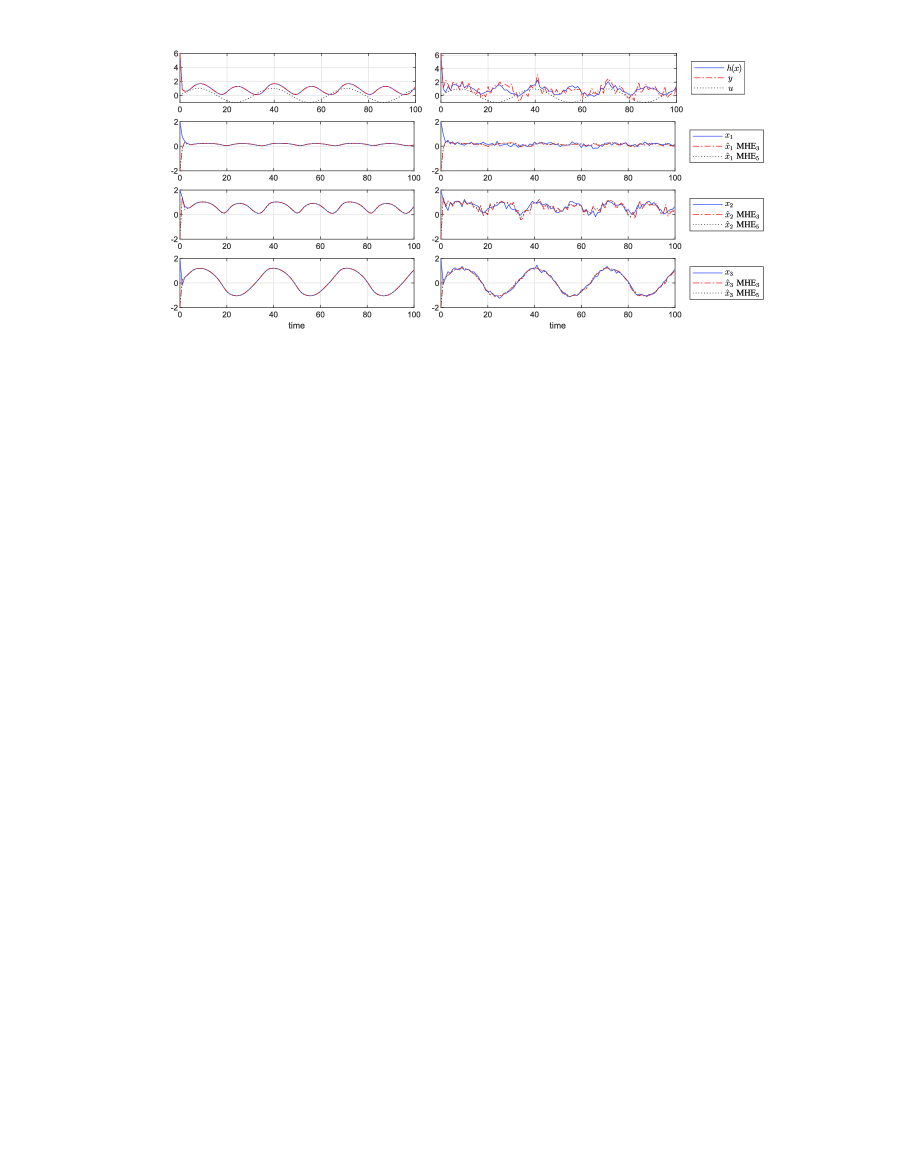
Figure 1: State and estimated state variables of MHE₃ (with fmincon and $\varepsilon=0.01$) and MHE₅ (with fminimax and $\varepsilon=0.01$) in noise-free (on the left) and noisy (on the right, zero-mean Gaussian noises with dispersions equal to $0.1$ and $0.5$ for system and measurement disturbances, respectively) simulation runs with $x_{0}=(2\,,\,2\,,\,2)$, $\hat{x}_{0}=(-2\,,\,-2\,,\,-2)$, and $u_{t}=\sin(0.2\,t)$.

4.2 Not Exponential i-UIOSS Example

Figure 2: State and estimated state variables of MHE₃ and MHE₄ with multi-start search fminimax in noise-free (on the left) and noisy simulation runs (on the right, with uniformly distributed random noises in $[-0.01,0.01]$ and $[-0.5,0.5]$ for system and measurement disturbances, respectively) with $x_{0}=(1\,,\,1)$ and $\hat{x}_{0}=(-1\,,\,-1)$.

The second-order system

$$\begin{array}[]{l}f(x,w)=\Bigg{(}\displaystyle\frac{x_{1}}{\sqrt{x_{1}^{2}+1}}+0.1\,x_{2}^{2}\,,\,0.5\sin(x_{2})+w\Bigg{)}\in{\mathop{\mathbb{R}}}^{2}\\ h(x,v)=x_{1}+x_{2}^{2}+\arctan\left(x_{1}+x_{2}\right)v\in{\mathop{\mathbb{R}}}\end{array}$$ (78)

with disturbances $w,v\in{\mathop{\mathbb{R}}}$ is not i-UEIOSS since the solution with $w\equiv 0,v\equiv 0$ and initial conditions $(\xi_{0},0)$, $\xi_{0}\not=0$ is

$$x_{t}=\left(\frac{\xi_{0}}{\sqrt{t\,\xi_{0}^{2}+1}}\,,\,0\right)\,,\,t=0,1,\ldots$$

and thus $|x_{t}|$ decreases to zero slower than exponential [24, Example 3, p. 3419]. To deal with such a system affected by the multiplicative measurement noise $v$, we need a simple extension of [22, Proposition 5, p. 4499] for systems described by (1) by proving that (2) in Definition 1 holds for some $\beta_{x}$, $\beta_{y}$, $\beta_{v}$, $\beta_{w}\in{\mathcal{K}L}$ if there exist $V:\mathbb{X}\times\mathbb{X}\rightarrow{\mathop{\mathbb{R}}}_{\geq 0}$ and $\alpha_{1},\alpha_{2},\alpha_{3}\in{\mathcal{K}}_{\infty}$, $\sigma_{w},\sigma_{y},\sigma_{v}\in{\mathcal{K}}$ such that

$$\alpha_{1}(|x-z|)\leq V(x,z)\leq\alpha_{2}(|x-z|)$$ (79)

$$V\left(f(x,u,w_{x}),f(z,u,w_{z})\right)\leq V(x,z)-\alpha_{3}(|x-z|)+\sigma_{w}(|w_{x}-w_{z}|)+\sigma_{y}\left(|h(x,v_{x})-h(z,v_{z})|\right)$$

$$\qquad\qquad\qquad\qquad\qquad\qquad+\sigma_{v}\left(|v_{x}-v_{z}|\right)$$ (80)

for all $x,z\in\mathbb{X}$, $w_{x},w_{z}\in\mathbb{W}$, and $v_{x},v_{z}\in\mathbb{V}$. More specifically, there exists $\sigma\in{\mathcal{K}}_{\infty}$ such that $\sigma(s)<s$ and

$$|x_{t}-z_{t}|\leq\overbrace{\alpha_{1}^{-1}(\beta(\alpha_{2}(|x_{0}-z_{0}|),t))}^{\beta_{x}(|x_{0}-z_{0}|,t)}\oplus\scalebox{1.5}{$\oplus$}_{i=0}^{t-1}\overbrace{\alpha_{1}^{-1}(\beta(\phi_{w}(|{w_{x}}_{i}-{w_{z}}_{i}|),t\!-\!1\!-\!i))}^{\beta_{w}(|{w_{x}}_{i}-{w_{z}}_{i}|,t-1-i)}$$

$$\oplus\scalebox{1.5}{$\oplus$}_{i=0}^{t-1}\overbrace{\alpha_{1}^{-1}(\beta(\phi_{y}(|h(x_{i},{v_{x}}_{i})-h(z_{i},{v_{z}}_{i})|),t\!-\!1\!-\!i))}^{\beta_{y}(|h(x_{i},{v_{x}}_{i})-h(z_{i},{v_{z}}_{i})|,t-1-i)}\oplus\scalebox{1.5}{$\oplus$}_{i=0}^{t-1}\overbrace{\alpha_{1}^{-1}(\beta(\phi_{v}(|{v_{x}}_{i}-{v_{z}}_{i}|),t\!-\!1\!-\!i))}^{\beta_{v}(|{v_{x}}_{i}-{v_{z}}_{i}|,t-1-i)}\,,\,t=0,1,\ldots$$ (81)

where $\beta(s,k):=\sigma^{k}(s)$, $\phi_{\ell}(s):=3\,\alpha_{2}(\alpha_{3}^{-1}(6\,\sigma_{\ell}(s)))+3\,\sigma_{\ell}(s)$ for $\ell=w,y,v$ with $x_{t+1}=f(x_{t},{w_{x}}_{t})$, $z_{t+1}=f(z_{t},{w_{z}}_{t})$, ${w_{x}}_{t},{w_{z}}_{t}\in\mathbb{W}$, ${v_{x}}_{t},{v_{z}}_{t}\in\mathbb{V}$. The proof of (81) is in line with the proof of [22, Proposition 5, p. 4499] and it is omitted due to the space limitation.

To show that $V_{c_{1}}\!(x,z)=\ln(c_{1}|x-z|^{2}+1)$ is an i-UIOSS Lyapunov function for (78) with $\sigma_{c_{w}}\!(s)=c_{w}s$, $\sigma_{c_{y}}\!(s)=c_{y}s$, $\sigma_{c_{v}}\!(s)=c_{v}s$ and $x,z\in\mathbb{X}=[-2,2]\times[-2,2]$, $w_{x},w_{z}\in\mathbb{W}=[-0.01,0.01]$, and $v_{x},v_{z}\in\mathbb{V}=[-0.5,0.5]$, we solved the optimization problem

$$\max_{\begin{array}[]{c}\\[-5.69046pt] c\geq 0,x,\!z\!\in\!\mathbb{X},\\ w_{x},\!w_{z}\!\in\!\mathbb{W},v_{x},\!v_{z}\!\in\!\mathbb{V}\end{array}}\!\!\!\!\!\!\!\!F(c,x,z,w_{x},w_{z},v_{x},v_{z}) :=\frac{1}{V_{c_{1}}\!(x,z)}\Big{(}V_{c_{1}}\!\left(f(x,w_{x}),f(z,w_{z})\right)-\sigma_{c_{w}}\!(|w_{x}-w_{z}|)$$ (85)

$$\quad-\sigma_{c_{y}}\!\left(|h(x,v_{x})-h(z,v_{z})|\right)-\sigma_{c_{v}}\!\left(|v_{x}-v_{z}|\right)\Big{)}$$ (86)

where $c:=(c_{1}\,,\,c_{w}\,,\,c_{y}\,,\,c_{v})\in{\mathop{\mathbb{R}}}^{4}_{\geq 0}$ and checked that there exists a solution $c^{*},x^{*},z^{*},w_{x}^{*},w_{z}^{*},v_{x}^{*},v_{z}^{*}$ such that $c^{*}>0$ and $F(c^{*},x^{*},z^{*},w_{x}^{*},w_{z}^{*},v_{x}^{*},v_{z}^{*})\in(0,1)$. In such a case, we got $\alpha_{3}(s)=(1-c_{0}^{*})\ln(c_{1}^{*}s^{2}+1)$, where $c_{0}^{*}:=F(c^{*},x^{*},z^{*},w_{x}^{*},w_{z}^{*},v_{x}^{*},v_{z}^{*})$. Moreover, we chose $\alpha_{1}(s)=\alpha_{2}(s)=\ln(c_{1}^{*}s^{2}+1)$ as $s\mapsto\ln(c_{1}^{*}s^{2}+1)$ is increasing over $[0,+\infty)$. By using fmincon to solve (86), we obtained $c_{0}^{*}=0.8751$, $c_{1}^{*}=6.3899$, $c_{w}^{*}=5.0010$, $c_{y}^{*}=0.1822$, and $c_{v}^{*}=4.9997$; therefore, we got $\sigma(s)=(c_{0}^{*}+1)s/2$, from which it is straightforward to get $\beta_{x}(\cdot,\cdot),\beta_{w}(\cdot,\cdot),\beta_{y}(\cdot,\cdot),\beta_{v}(\cdot,\cdot)$ according to the definitions in (81) and thus cost (4). The results of noise-free and noisy simulation runs are shown in Fig. 2.

5 Conclusion

This paper presents novel insights on the robust stability of moving horizon estimators even in case of imperfect minimization of the cost function, which is an issue rarely addressed in the literature. In such a case, practical stability holds under the adoption of a suitable stopping criterion. This allows to trade off between accuracy and computational effort. The effectiveness of the proposed approach is illustrated by means of two case studies, with one of the two affected by a multiplicative noise. Future work will concern new prediction strategies in moving-horizon estimation for Lipschitz nonlinear systems [25] and the robust stability of fast moving-horizon estimators [17, 18].

References

• [1] D. Allan, J. Rawlings, and A. Teel, “Nonlinear detectability and incremental input/output-to-state stability,” SIAM Journal on Control and Optimization, vol. 59, no. 4, pp. 3017–3039, 2021.
• [2] E. Sontag, “Smooth stabilization implies coprime factorization,” IEEE Trans. on Automatic Control, vol. 34, no. 4, pp. 435–443, 1989.
• [3] E. Sontag and Y. Wang, “Output-to-state stability and detectability of nonlinear systems,” Systems & Control Letters, vol. 29, no. 5, pp. 279–290, 1997.
• [4] L. Ji, J. B. Rawlings, W. Hu, A. Wynn, and M. Diehl, “Robust stability of moving horizon estimation under bounded disturbances,” IEEE Trans. on Automatic Control, vol. 61, no. 11, pp. 3509–3514, 2016.
• [5] M. Müller, “Nonlinear moving horizon estimation in the presence of bounded disturbances,” Automatica, vol. 79, pp. 306–314, 2017.
• [6] D. Allan and J. Rawlings, “Robust stability of full information estimation,” SIAM Journal on Control and Optimization, vol. 59, no. 5, pp. 3472–3497, 2021.
• [7] S. Knüfer and M. Müller, “Robust global exponential stability for moving horizon estimation,” in 56th Annual Conference on Decision and Control, Miami, FL, USA, 2018, pp. 3477–3482.
• [8] ——, “Nonlinear full information and moving horizon estimation: Robust global asymptotic stability,” Automatica, vol. 150, p. 110603, 2023.
• [9] J. Schiller and M. Müller, “Suboptimal nonlinear moving horizon estimation,” IEEE Trans. on Automatic Control, vol. 68, no. 4, p. 2199–2214, 2023.
• [10] W. Hu, “Generic stability implication from full information estimation to moving-horizon estimation,” IEEE Trans. on Automatic Control, vol. 69, no. 2, pp. 1164–1170, 2024.
• [11] J. Schiller, S. Muntwiler, J. Köhler, M. Zeilinger, and M. Müller, “A Lyapunov function for robust stability of moving horizon estimation,” IEEE Trans. on Automatic Control, vol. 68, no. 12, pp. 7466–7481, 2023.
• [12] D. Angeli, “A Lyapunov approach to incremental stability properties,” IEEE Trans. on Automatic Control, vol. 47, no. 3, pp. 410–421, 2002.
• [13] ——, “Further results on incremental input-to-state stability,” IEEE Trans. on Automatic Control, vol. 54, no. 6, pp. 1386–1391, 2009.
• [14] D. Allan, “A Lyapunov-like function for analysis of model predictive control and moving horizon estimation,” Ph.D. dissertation, University of Wisconsin–Madison, 2020.
• [15] P. Kühl, M. Diehl, T. Kraus, J. Schlöder, and H. Bock, “A real-time algorithm for moving horizon state and parameter estimation,” Computers & Chemical Engineering, vol. 35, no. 1, pp. 71–83, 2011.
• [16] A. Wynn, M. Vukov, and M. Diehl, “Convergence guarantees for moving horizon estimation based on the real-time iteration scheme,” IEEE Trans. on Automatic Control, vol. 59, no. 8, pp. 2215–2221, 2014.
• [17] A. Alessandri and M. Gaggero, “Fast moving horizon state estimation for discrete-time systems using single and multi iteration descent methods,” IEEE Trans. on Automatic Control, vol. 62, no. 9, pp. 4499–4511, 2017.
• [18] ——, “Fast moving horizon state estimation for discrete-time systems with linear constraints,” Int. Journal of Adaptive Control and Signal Processing, vol. 34, no. 6, pp. 706–720, 2020.
• [19] M. Gharbi, B. Gharesifard, and C. Ebenbauer, “Anytime proximity moving horizon estimation: Stability and regret,” IEEE Trans. on Automatic Control, vol. 68, no. 6, p. 3393–3408, 2022.
• [20] T. Liu, K. Chakrabarti, and N. Chopra, “Iteratively preconditioned gradient-descent approach for moving horizon estimation problems,” in 62nd IEEE Conference on Decision and Control, 2023, pp. 8457–8462.
• [21] D. Bertsekas, Nonlinear Programming. Belmont, MA: Athena Scientific, 1999.
• [22] D. Allan and J. Rawlings, “A Lyapunov-like function for full information estimation,” in 2019 American Control Conference (ACC), Miami, FL, USA, 2019, p. 4497–4502.
• [23] J. Rawlings, D. Mayne, and M. Diehl, Model Predictive Control: Theory, Computation, and Design. Madison, WI: Nob Hill Publishing, 2017.
• [24] D. Tran, B. Rüffer, and C. Kellett, “Convergence properties for discrete-time nonlinear systems,” IEEE Trans. on Automatic Control, vol. 64, no. 8, pp. 3415–3422, 2019.
• [25] H. Arezki, A. Zemouche, A. Alessandri, and P. Bagnerini, “LMI design procedure for incremental input/output-to-state stability in nonlinear systems,” IEEE Control Systems Letters, vol. 7, pp. 3403–3408, 2023.