Categorical Diffusion of Weighted Lattices

Robert Ghrist, Miguel Lopez, Paige Randall North, and Hans Riess
(February 5, 2025)
Abstract

We introduce a categorical formalization of diffusion, motivated by data science and information dynamics. Central to our construction is the Lawvere Laplacian, an endofunctor on a product category indexed by a graph and enriched in a quantale. This framework permits the systematic study of diffusion processes on network sheaves taking values in a class of enriched categories.

1 Introduction

Laplacians are ubiquitous. In calculus, the Laplacian is defined in terms of grad and div (and star). This culminates in Hodge theory via the the exterior derivative on differential forms, i.e. the de Rham complex with $d$ as a coboundary operator. More generally, the Laplace-Beltrami operator generalizes the classical Laplace operator to (pseudo-) Riemannian manifolds: this is the Hodge Laplacian in degree zero. In PDEs, the Laplacian determines harmonic functions, binding geometric and spectral data.

In discrete mathematics, from combinatorics to network and data science, the graph Laplacian drives everything from spectral graph theory to the graph connection Laplacian and beyond. These converge in probability to the Laplace-Beltrami operator and the connection Laplacian as the number of vertices of the graph approximating a manifold approaches infinity [38, 5].

In the context of a simplicial or cell complex, it has been known (somewhat as a folk theorem) that the Hodge Laplacian and the corresponding isomorphism between the cochain groups and $\operatorname{im}{d}\oplus\operatorname{im}{d^{\ast}}\oplus\ker(L)$ holds true in the general context of complexes whose chain groups are Hilbert spaces [15]. A recent merger of the simplicial and Hodge Laplacian has sparked a flurry of applications in applied mathematics, including distributed optimization, image processing, machine learning, opinion dynamics, random walks, spectral graph theory, synchronization, and more [4, 7, 22, 23, 27, 33, 35, 40].

The extension from a graph Laplacian diffusing scalar-valued data over graph vertices to vector-valued data is mostly straightforward [22], with the graph connection Laplacian [38] being a simple but useful instance of the more general Hodge Laplacian on a cellular sheaf of vector spaces over a graph — network sheaves. The quiver Laplacian generalizes the base of network sheaves from undirected graphs to arbitrary quivers [40]. Extending from vector-valued data to more general data categories poses significant challenges, especially when the data category is not abelian [21]. The introduction of the Tarski Laplacian in 2022 presented an operator on cellular sheaf cochains that take values in the category of complete order lattices with Galois connections as morphisms [19, 32]. This Tarski Laplacian was shown to enact discrete-time diffusion: cochains converge to harmonic cochains over time, thanks to the Tarski Fixed Point Theorem [42].

The primary goal of this paper is to generalize Laplacians to systems with data valued in more general enriched categories. We call the resulting operator the Lawvere Laplacian after Lawvere’s seminal work connecting enriched categories to metric spaces [26]. Along the way we develop several surprising analogies between linear and enriched categorical algebra. Moreover, we find that categorical enrichment is an apt framework for ‘fuzzy’ category theory, where one can explore approximate functors and adjunctions.

1.1 Towards Categorical Diffusion

Given a small category $\mathcal{G}$ and a presheaf $F:\mathcal{G}^{\mathrm{op}}\to\mathsf{Data}$ for some category of data, we would like a suitable notion of a Laplacian operator associated to $F$. In particular, we would like a map $L:C^{\bullet}F\to C^{\bullet}F$ where $C^{\bullet}F=\prod_{\sigma\in\mathcal{G}^{\mathrm{op}}}F(\sigma)$ is the total or cochain category of all the data stored above $\mathcal{G}$. In order for this map to model diffusion, we are guided by the following familiar properties witnessed by the numerous examples of Laplacians in other contexts [27, 22, 19, 40, 38].

1.1.1 Locality

The value of $L$ at an object $\sigma$ should only depend on the objects for which there is a transport morphism $F_{\tau\to\sigma}$, that is, the image of some morphism $\tau\to\sigma$ in $\mathcal{G}$. In other words, the $\sigma$-component of $L$ should be factorable as $L_{\sigma}:\prod_{\tau\to\sigma}F(\tau)\to F(\sigma)$ so that $L=\coprod_{\sigma}L_{\sigma}$. For instance, the quiver Laplacian at $\sigma$ is defined this way: the Laplacian depends only on those directed edges in $\sigma$. In PDEs like the heat equation, locality means that the evolution at a point depends only on its infinitesimal neighborhood in space. Likewise, for undirected discrete spaces, such as graphs, we take ’local’ to mean that the Laplacian should depend only on the data in a one-hop neighborhood of a node. This transition between continuous and discrete locality is exacted in approximation results for the Laplace-Beltrami operator and graph Laplacian [5], as well as the connection Laplacian and graph connection Laplacian [38] (modeling scalar and vector diffusion respectively).

1.1.2 Graphs

These approximation results motivate a theory of categorical diffusion over a preorder, which can capture the incidence relations of a combinatorial graph $G=(V,E)$ approximating a manifold. As such, our categorification targets combinatorial Hodge theory. Our dynamics are defined over categories $\mathcal{G}$ whose object set $\mathrm{ob}(\mathcal{G})=V\sqcup E$ consists of vertices and edges where morphisms are given by the incidence poset. While we are only interested in evolving the data over the vertices $C^{0}F:=\textstyle\prod_{v\in V}F(v)$, we can use the edges $C^{1}F:=\textstyle\prod_{e\in E}F(e)$ as way of comparing the pairwise consistency of vertex assignments.

1.1.3 Monotonicity

In linear algebraic contexts, the simplicial, quiver, sheaf, and Hodge Laplacians all have advantageous spectral properties, enabling the associated heat equations to converge. In particular, they are positive semi-definite linear operators, which we express suggestively by the property that $\langle Lx,x\rangle\geq 0$ for all $x\in C^{\bullet}F$. The heat equation

$$\frac{dx}{dt}=-\alpha Lx\quad:\quad\alpha>0$$ (1)

then satisfies $\langle Lx(t),x(t)\rangle\to 0$ monotonically as $t\to\infty$. Analogously, the Tarski Laplacian enjoys the property of being a decreasing operator: $x\geq Lx$ for all $x\in C^{\bullet}F$. We may suggestively write this as $\hom_{C^{\bullet}F}(Lx,x)\geq 1$ where $\hom_{C^{\bullet}F}:C^{\bullet}F^{\mathrm{op}}\times C^{\bullet}F\to\{0,1\}$ encodes the order structure of the cochain lattice. In this setting, the analogous (discrete-time) heat equation

$$x_{n+1}=x_{n}\wedge Lx_{n}=(I\wedge L)x_{n}$$

satisfies the condition that $\hom_{C^{\bullet}F}(x_{n},Lx_{n})$ increases monotonically from 0 to 1 when a fixed point of $I\wedge L$ is reached.

1.1.4 Completeness

Assuming that $C^{\bullet}F$ is ‘complete’ in some sense enables existence theorems for fixed points of the heat equation associated to $L$. In a typical linear algebraic setting, such operators $L$ are between finite dimensional Hilbert spaces which are complete as metric spaces. In the setting of the Tarski Laplacian, one considers $L$ as a map between complete lattices, or equivalently, small categories which are complete and cocomplete [16]. This assumption, together with Tarski’s fixed point theorem, guarantees existence and completeness of the resulting lattice of fixed points.

1.1.5 Adjoints

Comparing the hom bifunctor of a category with the inner product of a Hilbert space leads to an analogy between adjoint linear operators and adjoint functors. While we are not the first to compare these (e.g. see [1]), the analogy is most apparent in the context of $\mathsf{Q}$-categories where hom takes on a value in a quantale such as $[0,\infty]$. Linear adjoints are fundamental in establishing the global monotonicity property of linear algebraic Laplacians. At the local level, they appear as a mechanism for reversing maps so that ‘messages’ may be passed between nodes of a graph by first applying a forward map that pushes data from a given node to an incident edge, and then applying the transpose of another such map to pull the data back to the node level. The composition of these maps leads to a generalized notion of parallel transport, as evidenced by the graph connection Laplacian [38]. More generally, the structure of a network sheaf and a network cosheaf can facilitate almost any kind of graph message-passing scheme [6]. Thus, while adjunctions are not necessary to merely pass data back and forth, they are necessary for the Laplacian to capture harmonic (i.e. globally consistent) cochains both in the linear and lattice-theoretic setting.

1.2 Summary of Results

In Section 2, we develop the theory of categories enriched over commutative unital quantales $\mathsf{Q}$. Our primary contribution in this section is Theorem 2.17, which generalizes Tarski’s fixed point theorem to $\mathsf{Q}$-enriched categories. This theorem establishes that for any $\mathsf{Q}$-endofunctor on a weighted lattice (complete $\mathsf{Q}$-category), both the categories of prefix and suffix points are complete and non-empty. This result forms the theoretical foundation for our diffusion framework.

In Section 3, we introduce network sheaves valued in $\mathsf{Q}$-categories and develop the Lawvere Laplacian. We first show that fuzzy global sections can be characterized through weighted limits indexed by edge and vertex weightings. We then introduce $q$-fuzzy adjunctions between $\mathsf{Q}$-categories, which allow for controlled degradation in the transportation of data. Using these adjunctions, we construct the Lawvere Laplacian and prove that its suffix points approximate fuzzy global sections with error bounded by elements $q$ in a quantale. This provides a quantitative bridge between sheaf-theoretic and dynamical perspectives on network diffusion.

In Section 4, we demonstrate two applications of our framework. First, we show how the Lawvere Laplacian provides a categorical interpretation of classical path-finding algorithms, generalizing them to handle approximate computations. Second, we develop a theory of preference diffusion where fuzzy adjoints control the influence between agents’ preference relations.

The appendix provides technical background on $\mathsf{Q}$-categories and their weighted limits, including several novel results on the interaction between fuzzy adjunctions and weighted colimits that may be of independent interest.

2 Quantale-enriched Categories

Quantales are partially ordered sets that will serve as our system of coefficients for diffusion. The starting point of this paper is the well-known observation that a unital quantale can serve as the basis of categorical enrichment and with this, we can generalize the notion of lattice. With this perspective, lattices are certain categories enriched in the quantale of booleans (that is, the set $\{0,1\}$ with order and multiplication inherited from the natural numbers), and thus, in this sense, the Tarski Laplacian of [19, 32] uses coefficients from the booleans. In this paper, we allow coefficients from any commutative unital quantale. This captures many important mathematical objects, such as preordered sets, metric spaces, tropical semi-modules, etc. We use this section to review the basic theory of quantales and quantale-enriched categories as the foundation of our theory of categorical diffusion.

2.1 Quantales

Recall that a suplattice is a partially ordered set (also called poset) $(Q,\preceq)$ with suprema of all subsets. We denote the supremum of a subset $\{q_{i}\}_{i\in I}\subseteq Q$ with the symbol $\textstyle\bigvee_{i\in I}q_{i}$ or by $\textstyle\bigvee\{q_{i}\}_{i\in I}$. A suplattice also has infima of all subsets: given $\{q_{i}\}_{i\in I}\subseteq Q$, the infimum is $\textstyle\bigvee\{p:p\preceq q_{i}~\forall i\in I\}$. We denote such an infimum as $\textstyle\bigwedge_{i\in I}q_{i}$. To emphasize the symmetry (i.e., that suplattices have both infima and suprema), we also call them complete lattices. We write $\top=\textstyle\bigvee Q$ and $\bot=\textstyle\bigvee\emptyset$ for the top (a.k.a. the maximum or terminal object) and bottom (a.k.a. the minimum or initial object) elements of $Q$.

A quantale is a suplattice $Q$ together with an associative binary operation $\,\smash{\raisebox{0.80002pt}{$\scriptscriptstyle\bullet$}}\,:Q\times Q\to Q$ such that for all $p\in Q$ and for all $\{q_{i}\}_{i\in I}\subseteq Q$,

$\displaystyle\begin{aligned} p\,\smash{\raisebox{0.80002pt}{$\scriptscriptstyle\bullet$}}\,\Bigl{(}\textstyle\bigvee_{i\in I}q_{i}\Bigr{)}&=\textstyle\bigvee_{i\in I}(p\,\smash{\raisebox{0.80002pt}{$\scriptscriptstyle\bullet$}}\,q_{i});\quad\Bigl{(}\textstyle\bigvee_{i\in I}q_{i}\Bigr{)}\,\smash{\raisebox{0.80002pt}{$\scriptscriptstyle\bullet$}}\,p&=\textstyle\bigvee_{i\in I}(q_{i}\,\smash{\raisebox{0.80002pt}{$\scriptscriptstyle\bullet$}}\,p).\end{aligned}$ (2)

We say a quantale $(Q,\preceq,\,\smash{\raisebox{0.80002pt}{$\scriptscriptstyle\bullet$}}\,)$ is unital if the binary operation has a unit, commutative if the operation is commutative (i.e. symmetric), semicartesian if $p\,\smash{\raisebox{0.80002pt}{$\scriptscriptstyle\bullet$}}\,q\preceq p\wedge q$ for all $p,q\in Q$, and cartesian if the operation is the meet (that is, if $p\,\smash{\raisebox{0.80002pt}{$\scriptscriptstyle\bullet$}}\,q=p\wedge q$ for all $p,q\in Q$). Note that a semicartesian quantale has the affine property: the unit and terminal object coincide ($1=\top$).

We assume from now on that all quantales are unital, writing $\mathsf{Q}=(Q,\,\smash{\raisebox{0.80002pt}{$\scriptscriptstyle\bullet$}}\,,1,\preceq)$ for the data of a quantale given by the set of objects $\mathrm{ob}(\mathsf{Q})=Q$, binary operation  $\scriptscriptstyle\bullet$ , unit $1\in Q$, and order $p\preceq q$. For readers familiar with monoidal categories, note that $\mathsf{Q}$ is a thin, monoidal category.

2.1.1 Internal Homs

Because left and right multiplication are supmorphisms, by the adjoint functor theorem [29], quantales are endowed with left and right internal homs (also called residuals in the lattice context) defined by the following:

pq:={r:prq}pq:={r:rpq}\displaystyle\begin{aligned} p\,\leavevmode\hbox to11.78pt{\vbox to3.25pt{\pgfpicture\makeatletter\hbox{\thinspace\lower-1.62263pt\hbox to0.0pt{\pgfsys@beginscope\pgfsys@invoke{ }\definecolor{pgfstrokecolor}{rgb}{0,0,0}\pgfsys@color@rgb@stroke{0}{0}{0}\pgfsys@invoke{ }\pgfsys@color@rgb@fill{0}{0}{0}\pgfsys@invoke{ }\pgfsys@setlinewidth{0.4pt}\pgfsys@invoke{ }\nullfont\hbox to0.0pt{\pgfsys@beginscope\pgfsys@invoke{ }{}{{}}{} {{}{}}{}{{{{}{}{}{}}} {{{}{}{}{}}} {{{}{}{}{}}} {{}{}{}{}}}{} {} {}{}{}\pgfsys@moveto{0.0pt}{0.0pt}\pgfsys@lineto{8.53583pt}{0.0pt}\pgfsys@curveto{8.53583pt}{-0.7857pt}{9.17276pt}{-1.42264pt}{9.95847pt}{-1.42264pt}\pgfsys@curveto{10.74417pt}{-1.42264pt}{11.3811pt}{-0.7857pt}{11.3811pt}{0.0pt}\pgfsys@curveto{11.3811pt}{0.7857pt}{10.74417pt}{1.42264pt}{9.95847pt}{1.42264pt}\pgfsys@curveto{9.17276pt}{1.42264pt}{8.53583pt}{0.7857pt}{8.53583pt}{0.0pt}\pgfsys@stroke\pgfsys@invoke{ } \pgfsys@invoke{\lxSVG@closescope }\pgfsys@endscope{}{}{}\hss}\pgfsys@discardpath\pgfsys@invoke{\lxSVG@closescope }\pgfsys@endscope\hss}}\lxSVG@closescope\endpgfpicture}}\,q:=\bigvee\big{\{}r:p\,\smash{\raisebox{0.80002pt}{$\scriptscriptstyle\bullet$}}\,r\preceq q\big{\}}\\ p\,\leavevmode\hbox to10.36pt{\vbox to3.25pt{\pgfpicture\makeatletter\hbox{\thinspace\lower-1.62263pt\hbox to0.0pt{\pgfsys@beginscope\pgfsys@invoke{ }\definecolor{pgfstrokecolor}{rgb}{0,0,0}\pgfsys@color@rgb@stroke{0}{0}{0}\pgfsys@invoke{ }\pgfsys@color@rgb@fill{0}{0}{0}\pgfsys@invoke{ }\pgfsys@setlinewidth{0.4pt}\pgfsys@invoke{ }\nullfont\hbox to0.0pt{\pgfsys@beginscope\pgfsys@invoke{ }{{}{}}{{}}{}{{{{}{}{}{}}} {{{}{}{}{}}} {{{}{}{}{}}} {{}{}{}{}}}{} {} {}{} {{}{}}{}{}\pgfsys@moveto{1.42264pt}{0.0pt}\pgfsys@curveto{1.42264pt}{0.7857pt}{0.7857pt}{1.42264pt}{0.0pt}{1.42264pt}\pgfsys@curveto{-0.7857pt}{1.42264pt}{-1.42264pt}{0.7857pt}{-1.42264pt}{0.0pt}\pgfsys@curveto{-1.42264pt}{-0.7857pt}{-0.7857pt}{-1.42264pt}{0.0pt}{-1.42264pt}\pgfsys@curveto{0.7857pt}{-1.42264pt}{1.42264pt}{-0.7857pt}{1.42264pt}{0.0pt}\pgfsys@lineto{8.53583pt}{0.0pt}\pgfsys@stroke\pgfsys@invoke{ } \pgfsys@invoke{\lxSVG@closescope }\pgfsys@endscope{}{}{}\hss}\pgfsys@discardpath\pgfsys@invoke{\lxSVG@closescope }\pgfsys@endscope\hss}}\lxSVG@closescope\endpgfpicture}}\,q:=\bigvee\big{\{}r:r\,\smash{\raisebox{0.80002pt}{$\scriptscriptstyle\bullet$}}\,p\preceq q\big{\}}\end{aligned} (3)

for $p,q\in Q$. If $\mathsf{Q}$ is commutative, then the right and left internal hom coincide: in that case, we denote the internal hom by $[p,q]$. We will use the following standard properties of the internal hom:

Lemma 2.1.

In any quantale $\mathsf{Q}=(Q,\,\smash{\raisebox{0.80002pt}{$\scriptscriptstyle\bullet$}}\,,1,\preceq)$, for elements $p,q,r\in Q$, and a subset $\{q_{i}\}_{i\in I}\subseteq Q$ we have the following.

  1. 1.

    If $q\preceq r$, then pqprp\,\leavevmode\hbox to11.78pt{\vbox to3.25pt{\pgfpicture\makeatletter\hbox{\thinspace\lower-1.62263pt\hbox to0.0pt{\pgfsys@beginscope\pgfsys@invoke{ }\definecolor{pgfstrokecolor}{rgb}{0,0,0}\pgfsys@color@rgb@stroke{0}{0}{0}\pgfsys@invoke{ }\pgfsys@color@rgb@fill{0}{0}{0}\pgfsys@invoke{ }\pgfsys@setlinewidth{0.4pt}\pgfsys@invoke{ }\nullfont\hbox to0.0pt{\pgfsys@beginscope\pgfsys@invoke{ }{}{{}}{} {{}{}}{}{{{{}{}{}{}}} {{{}{}{}{}}} {{{}{}{}{}}} {{}{}{}{}}}{} {} {}{}{}\pgfsys@moveto{0.0pt}{0.0pt}\pgfsys@lineto{8.53583pt}{0.0pt}\pgfsys@curveto{8.53583pt}{-0.7857pt}{9.17276pt}{-1.42264pt}{9.95847pt}{-1.42264pt}\pgfsys@curveto{10.74417pt}{-1.42264pt}{11.3811pt}{-0.7857pt}{11.3811pt}{0.0pt}\pgfsys@curveto{11.3811pt}{0.7857pt}{10.74417pt}{1.42264pt}{9.95847pt}{1.42264pt}\pgfsys@curveto{9.17276pt}{1.42264pt}{8.53583pt}{0.7857pt}{8.53583pt}{0.0pt}\pgfsys@stroke\pgfsys@invoke{ } \pgfsys@invoke{\lxSVG@closescope }\pgfsys@endscope{}{}{}\hss}\pgfsys@discardpath\pgfsys@invoke{\lxSVG@closescope }\pgfsys@endscope\hss}}\lxSVG@closescope\endpgfpicture}}\,q\preceq p\,\leavevmode\hbox to11.78pt{\vbox to3.25pt{\pgfpicture\makeatletter\hbox{\thinspace\lower-1.62263pt\hbox to0.0pt{\pgfsys@beginscope\pgfsys@invoke{ }\definecolor{pgfstrokecolor}{rgb}{0,0,0}\pgfsys@color@rgb@stroke{0}{0}{0}\pgfsys@invoke{ }\pgfsys@color@rgb@fill{0}{0}{0}\pgfsys@invoke{ }\pgfsys@setlinewidth{0.4pt}\pgfsys@invoke{ }\nullfont\hbox to0.0pt{\pgfsys@beginscope\pgfsys@invoke{ }{}{{}}{} {{}{}}{}{{{{}{}{}{}}} {{{}{}{}{}}} {{{}{}{}{}}} {{}{}{}{}}}{} {} {}{}{}\pgfsys@moveto{0.0pt}{0.0pt}\pgfsys@lineto{8.53583pt}{0.0pt}\pgfsys@curveto{8.53583pt}{-0.7857pt}{9.17276pt}{-1.42264pt}{9.95847pt}{-1.42264pt}\pgfsys@curveto{10.74417pt}{-1.42264pt}{11.3811pt}{-0.7857pt}{11.3811pt}{0.0pt}\pgfsys@curveto{11.3811pt}{0.7857pt}{10.74417pt}{1.42264pt}{9.95847pt}{1.42264pt}\pgfsys@curveto{9.17276pt}{1.42264pt}{8.53583pt}{0.7857pt}{8.53583pt}{0.0pt}\pgfsys@stroke\pgfsys@invoke{ } \pgfsys@invoke{\lxSVG@closescope }\pgfsys@endscope{}{}{}\hss}\pgfsys@discardpath\pgfsys@invoke{\lxSVG@closescope }\pgfsys@endscope\hss}}\lxSVG@closescope\endpgfpicture}}\,r. Dually, if $p\preceq r$, then pqrqp\,\leavevmode\hbox to11.78pt{\vbox to3.25pt{\pgfpicture\makeatletter\hbox{\thinspace\lower-1.62263pt\hbox to0.0pt{\pgfsys@beginscope\pgfsys@invoke{ }\definecolor{pgfstrokecolor}{rgb}{0,0,0}\pgfsys@color@rgb@stroke{0}{0}{0}\pgfsys@invoke{ }\pgfsys@color@rgb@fill{0}{0}{0}\pgfsys@invoke{ }\pgfsys@setlinewidth{0.4pt}\pgfsys@invoke{ }\nullfont\hbox to0.0pt{\pgfsys@beginscope\pgfsys@invoke{ }{}{{}}{} {{}{}}{}{{{{}{}{}{}}} {{{}{}{}{}}} {{{}{}{}{}}} {{}{}{}{}}}{} {} {}{}{}\pgfsys@moveto{0.0pt}{0.0pt}\pgfsys@lineto{8.53583pt}{0.0pt}\pgfsys@curveto{8.53583pt}{-0.7857pt}{9.17276pt}{-1.42264pt}{9.95847pt}{-1.42264pt}\pgfsys@curveto{10.74417pt}{-1.42264pt}{11.3811pt}{-0.7857pt}{11.3811pt}{0.0pt}\pgfsys@curveto{11.3811pt}{0.7857pt}{10.74417pt}{1.42264pt}{9.95847pt}{1.42264pt}\pgfsys@curveto{9.17276pt}{1.42264pt}{8.53583pt}{0.7857pt}{8.53583pt}{0.0pt}\pgfsys@stroke\pgfsys@invoke{ } \pgfsys@invoke{\lxSVG@closescope }\pgfsys@endscope{}{}{}\hss}\pgfsys@discardpath\pgfsys@invoke{\lxSVG@closescope }\pgfsys@endscope\hss}}\lxSVG@closescope\endpgfpicture}}\,q\succeq r\,\leavevmode\hbox to11.78pt{\vbox to3.25pt{\pgfpicture\makeatletter\hbox{\thinspace\lower-1.62263pt\hbox to0.0pt{\pgfsys@beginscope\pgfsys@invoke{ }\definecolor{pgfstrokecolor}{rgb}{0,0,0}\pgfsys@color@rgb@stroke{0}{0}{0}\pgfsys@invoke{ }\pgfsys@color@rgb@fill{0}{0}{0}\pgfsys@invoke{ }\pgfsys@setlinewidth{0.4pt}\pgfsys@invoke{ }\nullfont\hbox to0.0pt{\pgfsys@beginscope\pgfsys@invoke{ }{}{{}}{} {{}{}}{}{{{{}{}{}{}}} {{{}{}{}{}}} {{{}{}{}{}}} {{}{}{}{}}}{} {} {}{}{}\pgfsys@moveto{0.0pt}{0.0pt}\pgfsys@lineto{8.53583pt}{0.0pt}\pgfsys@curveto{8.53583pt}{-0.7857pt}{9.17276pt}{-1.42264pt}{9.95847pt}{-1.42264pt}\pgfsys@curveto{10.74417pt}{-1.42264pt}{11.3811pt}{-0.7857pt}{11.3811pt}{0.0pt}\pgfsys@curveto{11.3811pt}{0.7857pt}{10.74417pt}{1.42264pt}{9.95847pt}{1.42264pt}\pgfsys@curveto{9.17276pt}{1.42264pt}{8.53583pt}{0.7857pt}{8.53583pt}{0.0pt}\pgfsys@stroke\pgfsys@invoke{ } \pgfsys@invoke{\lxSVG@closescope }\pgfsys@endscope{}{}{}\hss}\pgfsys@discardpath\pgfsys@invoke{\lxSVG@closescope }\pgfsys@endscope\hss}}\lxSVG@closescope\endpgfpicture}}\,q.

  2. 2.

    We have p(iIqi)=iI(pqi)p\,\leavevmode\hbox to11.78pt{\vbox to3.25pt{\pgfpicture\makeatletter\hbox{\thinspace\lower-1.62263pt\hbox to0.0pt{\pgfsys@beginscope\pgfsys@invoke{ }\definecolor{pgfstrokecolor}{rgb}{0,0,0}\pgfsys@color@rgb@stroke{0}{0}{0}\pgfsys@invoke{ }\pgfsys@color@rgb@fill{0}{0}{0}\pgfsys@invoke{ }\pgfsys@setlinewidth{0.4pt}\pgfsys@invoke{ }\nullfont\hbox to0.0pt{\pgfsys@beginscope\pgfsys@invoke{ }{}{{}}{} {{}{}}{}{{{{}{}{}{}}} {{{}{}{}{}}} {{{}{}{}{}}} {{}{}{}{}}}{} {} {}{}{}\pgfsys@moveto{0.0pt}{0.0pt}\pgfsys@lineto{8.53583pt}{0.0pt}\pgfsys@curveto{8.53583pt}{-0.7857pt}{9.17276pt}{-1.42264pt}{9.95847pt}{-1.42264pt}\pgfsys@curveto{10.74417pt}{-1.42264pt}{11.3811pt}{-0.7857pt}{11.3811pt}{0.0pt}\pgfsys@curveto{11.3811pt}{0.7857pt}{10.74417pt}{1.42264pt}{9.95847pt}{1.42264pt}\pgfsys@curveto{9.17276pt}{1.42264pt}{8.53583pt}{0.7857pt}{8.53583pt}{0.0pt}\pgfsys@stroke\pgfsys@invoke{ } \pgfsys@invoke{\lxSVG@closescope }\pgfsys@endscope{}{}{}\hss}\pgfsys@discardpath\pgfsys@invoke{\lxSVG@closescope }\pgfsys@endscope\hss}}\lxSVG@closescope\endpgfpicture}}\,\left(\textstyle\bigwedge_{i\in I}q_{i}\right)=\bigwedge_{i\in I}(p\,\leavevmode\hbox to11.78pt{\vbox to3.25pt{\pgfpicture\makeatletter\hbox{\thinspace\lower-1.62263pt\hbox to0.0pt{\pgfsys@beginscope\pgfsys@invoke{ }\definecolor{pgfstrokecolor}{rgb}{0,0,0}\pgfsys@color@rgb@stroke{0}{0}{0}\pgfsys@invoke{ }\pgfsys@color@rgb@fill{0}{0}{0}\pgfsys@invoke{ }\pgfsys@setlinewidth{0.4pt}\pgfsys@invoke{ }\nullfont\hbox to0.0pt{\pgfsys@beginscope\pgfsys@invoke{ }{}{{}}{} {{}{}}{}{{{{}{}{}{}}} {{{}{}{}{}}} {{{}{}{}{}}} {{}{}{}{}}}{} {} {}{}{}\pgfsys@moveto{0.0pt}{0.0pt}\pgfsys@lineto{8.53583pt}{0.0pt}\pgfsys@curveto{8.53583pt}{-0.7857pt}{9.17276pt}{-1.42264pt}{9.95847pt}{-1.42264pt}\pgfsys@curveto{10.74417pt}{-1.42264pt}{11.3811pt}{-0.7857pt}{11.3811pt}{0.0pt}\pgfsys@curveto{11.3811pt}{0.7857pt}{10.74417pt}{1.42264pt}{9.95847pt}{1.42264pt}\pgfsys@curveto{9.17276pt}{1.42264pt}{8.53583pt}{0.7857pt}{8.53583pt}{0.0pt}\pgfsys@stroke\pgfsys@invoke{ } \pgfsys@invoke{\lxSVG@closescope }\pgfsys@endscope{}{}{}\hss}\pgfsys@discardpath\pgfsys@invoke{\lxSVG@closescope }\pgfsys@endscope\hss}}\lxSVG@closescope\endpgfpicture}}\,q_{i}). Dually, (iIqi)p=iI(qip)\left(\textstyle\bigvee_{i\in I}q_{i}\right)\,\leavevmode\hbox to11.78pt{\vbox to3.25pt{\pgfpicture\makeatletter\hbox{\thinspace\lower-1.62263pt\hbox to0.0pt{\pgfsys@beginscope\pgfsys@invoke{ }\definecolor{pgfstrokecolor}{rgb}{0,0,0}\pgfsys@color@rgb@stroke{0}{0}{0}\pgfsys@invoke{ }\pgfsys@color@rgb@fill{0}{0}{0}\pgfsys@invoke{ }\pgfsys@setlinewidth{0.4pt}\pgfsys@invoke{ }\nullfont\hbox to0.0pt{\pgfsys@beginscope\pgfsys@invoke{ }{}{{}}{} {{}{}}{}{{{{}{}{}{}}} {{{}{}{}{}}} {{{}{}{}{}}} {{}{}{}{}}}{} {} {}{}{}\pgfsys@moveto{0.0pt}{0.0pt}\pgfsys@lineto{8.53583pt}{0.0pt}\pgfsys@curveto{8.53583pt}{-0.7857pt}{9.17276pt}{-1.42264pt}{9.95847pt}{-1.42264pt}\pgfsys@curveto{10.74417pt}{-1.42264pt}{11.3811pt}{-0.7857pt}{11.3811pt}{0.0pt}\pgfsys@curveto{11.3811pt}{0.7857pt}{10.74417pt}{1.42264pt}{9.95847pt}{1.42264pt}\pgfsys@curveto{9.17276pt}{1.42264pt}{8.53583pt}{0.7857pt}{8.53583pt}{0.0pt}\pgfsys@stroke\pgfsys@invoke{ } \pgfsys@invoke{\lxSVG@closescope }\pgfsys@endscope{}{}{}\hss}\pgfsys@discardpath\pgfsys@invoke{\lxSVG@closescope }\pgfsys@endscope\hss}}\lxSVG@closescope\endpgfpicture}}\,p=\textstyle\bigwedge_{i\in I}\left(q_{i}\,\leavevmode\hbox to11.78pt{\vbox to3.25pt{\pgfpicture\makeatletter\hbox{\thinspace\lower-1.62263pt\hbox to0.0pt{\pgfsys@beginscope\pgfsys@invoke{ }\definecolor{pgfstrokecolor}{rgb}{0,0,0}\pgfsys@color@rgb@stroke{0}{0}{0}\pgfsys@invoke{ }\pgfsys@color@rgb@fill{0}{0}{0}\pgfsys@invoke{ }\pgfsys@setlinewidth{0.4pt}\pgfsys@invoke{ }\nullfont\hbox to0.0pt{\pgfsys@beginscope\pgfsys@invoke{ }{}{{}}{} {{}{}}{}{{{{}{}{}{}}} {{{}{}{}{}}} {{{}{}{}{}}} {{}{}{}{}}}{} {} {}{}{}\pgfsys@moveto{0.0pt}{0.0pt}\pgfsys@lineto{8.53583pt}{0.0pt}\pgfsys@curveto{8.53583pt}{-0.7857pt}{9.17276pt}{-1.42264pt}{9.95847pt}{-1.42264pt}\pgfsys@curveto{10.74417pt}{-1.42264pt}{11.3811pt}{-0.7857pt}{11.3811pt}{0.0pt}\pgfsys@curveto{11.3811pt}{0.7857pt}{10.74417pt}{1.42264pt}{9.95847pt}{1.42264pt}\pgfsys@curveto{9.17276pt}{1.42264pt}{8.53583pt}{0.7857pt}{8.53583pt}{0.0pt}\pgfsys@stroke\pgfsys@invoke{ } \pgfsys@invoke{\lxSVG@closescope }\pgfsys@endscope{}{}{}\hss}\pgfsys@discardpath\pgfsys@invoke{\lxSVG@closescope }\pgfsys@endscope\hss}}\lxSVG@closescope\endpgfpicture}}\,p\right).

  3. 3.

    1q=q1\,\leavevmode\hbox to11.78pt{\vbox to3.25pt{\pgfpicture\makeatletter\hbox{\thinspace\lower-1.62263pt\hbox to0.0pt{\pgfsys@beginscope\pgfsys@invoke{ }\definecolor{pgfstrokecolor}{rgb}{0,0,0}\pgfsys@color@rgb@stroke{0}{0}{0}\pgfsys@invoke{ }\pgfsys@color@rgb@fill{0}{0}{0}\pgfsys@invoke{ }\pgfsys@setlinewidth{0.4pt}\pgfsys@invoke{ }\nullfont\hbox to0.0pt{\pgfsys@beginscope\pgfsys@invoke{ }{}{{}}{} {{}{}}{}{{{{}{}{}{}}} {{{}{}{}{}}} {{{}{}{}{}}} {{}{}{}{}}}{} {} {}{}{}\pgfsys@moveto{0.0pt}{0.0pt}\pgfsys@lineto{8.53583pt}{0.0pt}\pgfsys@curveto{8.53583pt}{-0.7857pt}{9.17276pt}{-1.42264pt}{9.95847pt}{-1.42264pt}\pgfsys@curveto{10.74417pt}{-1.42264pt}{11.3811pt}{-0.7857pt}{11.3811pt}{0.0pt}\pgfsys@curveto{11.3811pt}{0.7857pt}{10.74417pt}{1.42264pt}{9.95847pt}{1.42264pt}\pgfsys@curveto{9.17276pt}{1.42264pt}{8.53583pt}{0.7857pt}{8.53583pt}{0.0pt}\pgfsys@stroke\pgfsys@invoke{ } \pgfsys@invoke{\lxSVG@closescope }\pgfsys@endscope{}{}{}\hss}\pgfsys@discardpath\pgfsys@invoke{\lxSVG@closescope }\pgfsys@endscope\hss}}\lxSVG@closescope\endpgfpicture}}\,q=q.

  4. 4.

    We have $q\preceq p$ if and only if 1qp1\preceq q\,\leavevmode\hbox to11.78pt{\vbox to3.25pt{\pgfpicture\makeatletter\hbox{\thinspace\lower-1.62263pt\hbox to0.0pt{\pgfsys@beginscope\pgfsys@invoke{ }\definecolor{pgfstrokecolor}{rgb}{0,0,0}\pgfsys@color@rgb@stroke{0}{0}{0}\pgfsys@invoke{ }\pgfsys@color@rgb@fill{0}{0}{0}\pgfsys@invoke{ }\pgfsys@setlinewidth{0.4pt}\pgfsys@invoke{ }\nullfont\hbox to0.0pt{\pgfsys@beginscope\pgfsys@invoke{ }{}{{}}{} {{}{}}{}{{{{}{}{}{}}} {{{}{}{}{}}} {{{}{}{}{}}} {{}{}{}{}}}{} {} {}{}{}\pgfsys@moveto{0.0pt}{0.0pt}\pgfsys@lineto{8.53583pt}{0.0pt}\pgfsys@curveto{8.53583pt}{-0.7857pt}{9.17276pt}{-1.42264pt}{9.95847pt}{-1.42264pt}\pgfsys@curveto{10.74417pt}{-1.42264pt}{11.3811pt}{-0.7857pt}{11.3811pt}{0.0pt}\pgfsys@curveto{11.3811pt}{0.7857pt}{10.74417pt}{1.42264pt}{9.95847pt}{1.42264pt}\pgfsys@curveto{9.17276pt}{1.42264pt}{8.53583pt}{0.7857pt}{8.53583pt}{0.0pt}\pgfsys@stroke\pgfsys@invoke{ } \pgfsys@invoke{\lxSVG@closescope }\pgfsys@endscope{}{}{}\hss}\pgfsys@discardpath\pgfsys@invoke{\lxSVG@closescope }\pgfsys@endscope\hss}}\lxSVG@closescope\endpgfpicture}}\,p. Thus, if $\mathsf{Q}$ is affine, then qp=1q\,\leavevmode\hbox to11.78pt{\vbox to3.25pt{\pgfpicture\makeatletter\hbox{\thinspace\lower-1.62263pt\hbox to0.0pt{\pgfsys@beginscope\pgfsys@invoke{ }\definecolor{pgfstrokecolor}{rgb}{0,0,0}\pgfsys@color@rgb@stroke{0}{0}{0}\pgfsys@invoke{ }\pgfsys@color@rgb@fill{0}{0}{0}\pgfsys@invoke{ }\pgfsys@setlinewidth{0.4pt}\pgfsys@invoke{ }\nullfont\hbox to0.0pt{\pgfsys@beginscope\pgfsys@invoke{ }{}{{}}{} {{}{}}{}{{{{}{}{}{}}} {{{}{}{}{}}} {{{}{}{}{}}} {{}{}{}{}}}{} {} {}{}{}\pgfsys@moveto{0.0pt}{0.0pt}\pgfsys@lineto{8.53583pt}{0.0pt}\pgfsys@curveto{8.53583pt}{-0.7857pt}{9.17276pt}{-1.42264pt}{9.95847pt}{-1.42264pt}\pgfsys@curveto{10.74417pt}{-1.42264pt}{11.3811pt}{-0.7857pt}{11.3811pt}{0.0pt}\pgfsys@curveto{11.3811pt}{0.7857pt}{10.74417pt}{1.42264pt}{9.95847pt}{1.42264pt}\pgfsys@curveto{9.17276pt}{1.42264pt}{8.53583pt}{0.7857pt}{8.53583pt}{0.0pt}\pgfsys@stroke\pgfsys@invoke{ } \pgfsys@invoke{\lxSVG@closescope }\pgfsys@endscope{}{}{}\hss}\pgfsys@discardpath\pgfsys@invoke{\lxSVG@closescope }\pgfsys@endscope\hss}}\lxSVG@closescope\endpgfpicture}}\,p=1. If $\mathsf{Q}$ is affine then qp=1q\,\leavevmode\hbox to11.78pt{\vbox to3.25pt{\pgfpicture\makeatletter\hbox{\thinspace\lower-1.62263pt\hbox to0.0pt{\pgfsys@beginscope\pgfsys@invoke{ }\definecolor{pgfstrokecolor}{rgb}{0,0,0}\pgfsys@color@rgb@stroke{0}{0}{0}\pgfsys@invoke{ }\pgfsys@color@rgb@fill{0}{0}{0}\pgfsys@invoke{ }\pgfsys@setlinewidth{0.4pt}\pgfsys@invoke{ }\nullfont\hbox to0.0pt{\pgfsys@beginscope\pgfsys@invoke{ }{}{{}}{} {{}{}}{}{{{{}{}{}{}}} {{{}{}{}{}}} {{{}{}{}{}}} {{}{}{}{}}}{} {} {}{}{}\pgfsys@moveto{0.0pt}{0.0pt}\pgfsys@lineto{8.53583pt}{0.0pt}\pgfsys@curveto{8.53583pt}{-0.7857pt}{9.17276pt}{-1.42264pt}{9.95847pt}{-1.42264pt}\pgfsys@curveto{10.74417pt}{-1.42264pt}{11.3811pt}{-0.7857pt}{11.3811pt}{0.0pt}\pgfsys@curveto{11.3811pt}{0.7857pt}{10.74417pt}{1.42264pt}{9.95847pt}{1.42264pt}\pgfsys@curveto{9.17276pt}{1.42264pt}{8.53583pt}{0.7857pt}{8.53583pt}{0.0pt}\pgfsys@stroke\pgfsys@invoke{ } \pgfsys@invoke{\lxSVG@closescope }\pgfsys@endscope{}{}{}\hss}\pgfsys@discardpath\pgfsys@invoke{\lxSVG@closescope }\pgfsys@endscope\hss}}\lxSVG@closescope\endpgfpicture}}\,p=1.

  5. 5.

    We have (pq)rp(qr)(p\,\leavevmode\hbox to11.78pt{\vbox to3.25pt{\pgfpicture\makeatletter\hbox{\thinspace\lower-1.62263pt\hbox to0.0pt{\pgfsys@beginscope\pgfsys@invoke{ }\definecolor{pgfstrokecolor}{rgb}{0,0,0}\pgfsys@color@rgb@stroke{0}{0}{0}\pgfsys@invoke{ }\pgfsys@color@rgb@fill{0}{0}{0}\pgfsys@invoke{ }\pgfsys@setlinewidth{0.4pt}\pgfsys@invoke{ }\nullfont\hbox to0.0pt{\pgfsys@beginscope\pgfsys@invoke{ }{}{{}}{} {{}{}}{}{{{{}{}{}{}}} {{{}{}{}{}}} {{{}{}{}{}}} {{}{}{}{}}}{} {} {}{}{}\pgfsys@moveto{0.0pt}{0.0pt}\pgfsys@lineto{8.53583pt}{0.0pt}\pgfsys@curveto{8.53583pt}{-0.7857pt}{9.17276pt}{-1.42264pt}{9.95847pt}{-1.42264pt}\pgfsys@curveto{10.74417pt}{-1.42264pt}{11.3811pt}{-0.7857pt}{11.3811pt}{0.0pt}\pgfsys@curveto{11.3811pt}{0.7857pt}{10.74417pt}{1.42264pt}{9.95847pt}{1.42264pt}\pgfsys@curveto{9.17276pt}{1.42264pt}{8.53583pt}{0.7857pt}{8.53583pt}{0.0pt}\pgfsys@stroke\pgfsys@invoke{ } \pgfsys@invoke{\lxSVG@closescope }\pgfsys@endscope{}{}{}\hss}\pgfsys@discardpath\pgfsys@invoke{\lxSVG@closescope }\pgfsys@endscope\hss}}\lxSVG@closescope\endpgfpicture}}\,q)\,\smash{\raisebox{0.80002pt}{$\scriptscriptstyle\bullet$}}\,r\preceq p\,\leavevmode\hbox to11.78pt{\vbox to3.25pt{\pgfpicture\makeatletter\hbox{\thinspace\lower-1.62263pt\hbox to0.0pt{\pgfsys@beginscope\pgfsys@invoke{ }\definecolor{pgfstrokecolor}{rgb}{0,0,0}\pgfsys@color@rgb@stroke{0}{0}{0}\pgfsys@invoke{ }\pgfsys@color@rgb@fill{0}{0}{0}\pgfsys@invoke{ }\pgfsys@setlinewidth{0.4pt}\pgfsys@invoke{ }\nullfont\hbox to0.0pt{\pgfsys@beginscope\pgfsys@invoke{ }{}{{}}{} {{}{}}{}{{{{}{}{}{}}} {{{}{}{}{}}} {{{}{}{}{}}} {{}{}{}{}}}{} {} {}{}{}\pgfsys@moveto{0.0pt}{0.0pt}\pgfsys@lineto{8.53583pt}{0.0pt}\pgfsys@curveto{8.53583pt}{-0.7857pt}{9.17276pt}{-1.42264pt}{9.95847pt}{-1.42264pt}\pgfsys@curveto{10.74417pt}{-1.42264pt}{11.3811pt}{-0.7857pt}{11.3811pt}{0.0pt}\pgfsys@curveto{11.3811pt}{0.7857pt}{10.74417pt}{1.42264pt}{9.95847pt}{1.42264pt}\pgfsys@curveto{9.17276pt}{1.42264pt}{8.53583pt}{0.7857pt}{8.53583pt}{0.0pt}\pgfsys@stroke\pgfsys@invoke{ } \pgfsys@invoke{\lxSVG@closescope }\pgfsys@endscope{}{}{}\hss}\pgfsys@discardpath\pgfsys@invoke{\lxSVG@closescope }\pgfsys@endscope\hss}}\lxSVG@closescope\endpgfpicture}}\,(q\,\smash{\raisebox{0.80002pt}{$\scriptscriptstyle\bullet$}}\,r) and r(pq)p(rq)r\,\smash{\raisebox{0.80002pt}{$\scriptscriptstyle\bullet$}}\,(p\,\leavevmode\hbox to10.36pt{\vbox to3.25pt{\pgfpicture\makeatletter\hbox{\thinspace\lower-1.62263pt\hbox to0.0pt{\pgfsys@beginscope\pgfsys@invoke{ }\definecolor{pgfstrokecolor}{rgb}{0,0,0}\pgfsys@color@rgb@stroke{0}{0}{0}\pgfsys@invoke{ }\pgfsys@color@rgb@fill{0}{0}{0}\pgfsys@invoke{ }\pgfsys@setlinewidth{0.4pt}\pgfsys@invoke{ }\nullfont\hbox to0.0pt{\pgfsys@beginscope\pgfsys@invoke{ }{{}{}}{{}}{}{{{{}{}{}{}}} {{{}{}{}{}}} {{{}{}{}{}}} {{}{}{}{}}}{} {} {}{} {{}{}}{}{}\pgfsys@moveto{1.42264pt}{0.0pt}\pgfsys@curveto{1.42264pt}{0.7857pt}{0.7857pt}{1.42264pt}{0.0pt}{1.42264pt}\pgfsys@curveto{-0.7857pt}{1.42264pt}{-1.42264pt}{0.7857pt}{-1.42264pt}{0.0pt}\pgfsys@curveto{-1.42264pt}{-0.7857pt}{-0.7857pt}{-1.42264pt}{0.0pt}{-1.42264pt}\pgfsys@curveto{0.7857pt}{-1.42264pt}{1.42264pt}{-0.7857pt}{1.42264pt}{0.0pt}\pgfsys@lineto{8.53583pt}{0.0pt}\pgfsys@stroke\pgfsys@invoke{ } \pgfsys@invoke{\lxSVG@closescope }\pgfsys@endscope{}{}{}\hss}\pgfsys@discardpath\pgfsys@invoke{\lxSVG@closescope }\pgfsys@endscope\hss}}\lxSVG@closescope\endpgfpicture}}\,q)\preceq p\,\leavevmode\hbox to10.36pt{\vbox to3.25pt{\pgfpicture\makeatletter\hbox{\thinspace\lower-1.62263pt\hbox to0.0pt{\pgfsys@beginscope\pgfsys@invoke{ }\definecolor{pgfstrokecolor}{rgb}{0,0,0}\pgfsys@color@rgb@stroke{0}{0}{0}\pgfsys@invoke{ }\pgfsys@color@rgb@fill{0}{0}{0}\pgfsys@invoke{ }\pgfsys@setlinewidth{0.4pt}\pgfsys@invoke{ }\nullfont\hbox to0.0pt{\pgfsys@beginscope\pgfsys@invoke{ }{{}{}}{{}}{}{{{{}{}{}{}}} {{{}{}{}{}}} {{{}{}{}{}}} {{}{}{}{}}}{} {} {}{} {{}{}}{}{}\pgfsys@moveto{1.42264pt}{0.0pt}\pgfsys@curveto{1.42264pt}{0.7857pt}{0.7857pt}{1.42264pt}{0.0pt}{1.42264pt}\pgfsys@curveto{-0.7857pt}{1.42264pt}{-1.42264pt}{0.7857pt}{-1.42264pt}{0.0pt}\pgfsys@curveto{-1.42264pt}{-0.7857pt}{-0.7857pt}{-1.42264pt}{0.0pt}{-1.42264pt}\pgfsys@curveto{0.7857pt}{-1.42264pt}{1.42264pt}{-0.7857pt}{1.42264pt}{0.0pt}\pgfsys@lineto{8.53583pt}{0.0pt}\pgfsys@stroke\pgfsys@invoke{ } \pgfsys@invoke{\lxSVG@closescope }\pgfsys@endscope{}{}{}\hss}\pgfsys@discardpath\pgfsys@invoke{\lxSVG@closescope }\pgfsys@endscope\hss}}\lxSVG@closescope\endpgfpicture}}\,(r\,\smash{\raisebox{0.80002pt}{$\scriptscriptstyle\bullet$}}\,q).

  6. 6.

    If $\mathsf{Q}$ is commutative, then $[p,[q,r]]=[p\,\smash{\raisebox{0.80002pt}{$\scriptscriptstyle\bullet$}}\,q,r]=[q,[p,r]]$.

Statements (1)-(4) are written for   , but the analogous laws (i.e. those obtained by replacing    with   ) hold for   .

Examples 2.2.

Quantales are encountered frequently. We compose a partial list of examples.

  1. 1.

    Cartesian quantales are also called frames (or locales).

  2. 2.

    Frames also include completely distributive lattices such as powersets.

  3. 3.

    In particular, the booleans $\mathsf{B}=(\{0,1\},\wedge,1,\leq)$ constitute a frame. The internal hom corresponds to implication $p\to q$ in the propositional calculus.

  4. 4.

    In fuzzy or multi-valued logic, monoidal operations on the unit interval are dubbed t-norms. These are required to make $\mathsf{I}=([0,1],\,\smash{\raisebox{0.80002pt}{$\scriptscriptstyle\bullet$}}\,,1,\leq)$ into a affine, commutative quantale (in terms of our vocabulary). Examples of t-norms include

    • $p\,\smash{\raisebox{0.80002pt}{$\scriptscriptstyle\bullet$}}\,q=p\times q$ (cf. Goguen fuzzy logic [20])

    • $p\,\smash{\raisebox{0.80002pt}{$\scriptscriptstyle\bullet$}}\,q=\max\{0,p+q-1\}$ (cf. Łukasiewicz fuzzy logic [28])

    • $p\,\smash{\raisebox{0.80002pt}{$\scriptscriptstyle\bullet$}}\,q=\min\{p,q\}$ (cf. Godel fuzzy logic [14])

    among many others.

  5. 5.

    The extended positive reals together with the reverse order and addition form a commutative, unital quantale, $\mathsf{R}=([0,\infty],+,0,\geq)$. The internal hom is given by $[p,q]=\max\{q-p,0\}$. Note that this is isomorphic to the quantale $\mathsf{I}=([0,1],\times,1,\leq)$ with the Goguen t-norm described above. On the underlying sets, this isomorphism $[0,1]\to[0,\infty]$ is given by $p\mapsto-\log(p)$.

  6. 6.

    The collection of ideals in a ring forms a quantale. In particular, if the ring is noncommutative, then its quantale of ideals is noncommutative.

  7. 7.

    For any quantale $Q$, the collection of $n\times n$ $Q$-matrices forms a quantale. Even if $Q$ is commutative, its associated matrix quantales are not (except in trivial cases) [17].

2.2 $\mathsf{Q}$-categories

Although many of the following results hold for categories enriched in arbitrary quantales, for simplicity we fix a semicartesian, unital, commutative quantale $\mathsf{Q}=(Q,\,\smash{\raisebox{0.80002pt}{$\scriptscriptstyle\bullet$}}\,,\preceq,1)$ for the remainder of the article, which in particular is affine.

Throughout this section, we cite [25] whenever our definitions or results are special cases of standard definitions or results in enriched category theory. However, since we are enriching over a quantale, and not a general monoidal category, our assumptions, terminology, and notation sometimes differ.

Definition 2.3 ([25, 1.2]).

A (small) $\mathsf{Q}$-category $\mathsf{C}$ consists of (i) a set $\mathrm{ob}(\mathsf{C})$ of objects and (ii) for each pair $x,y\in\mathrm{ob}(\mathsf{C})$, an element $\hom_{\mathsf{C}}(x,y)$ of $\mathsf{Q}$, such that

$\displaystyle\hom_{\mathsf{C}}(x,x)=1$ (4)

for all $x\in\mathrm{ob}(\mathsf{C})$, and

$\displaystyle\hom_{\mathsf{C}}(x,y)\,\smash{\raisebox{0.80002pt}{$\scriptscriptstyle\bullet$}}\,\hom_{\mathsf{C}}(y,z)\preceq\hom_{\mathsf{C}}(x,z)$ (5)

for all $x,y,z\in\mathrm{ob}(\mathsf{C})$. A $\mathsf{Q}$-functor $F:\mathsf{C}\to\mathsf{D}$ between $\mathsf{Q}$-categories $\mathsf{C}$ and $\mathsf{D}$ consists of a function $\mathrm{ob}(F):\mathrm{ob}(\mathsf{C})\to\mathrm{ob}(\mathsf{D})$ such that

$\displaystyle\hom_{\mathsf{C}}(x,y)\preceq\hom_{\mathsf{D}}(Fx,Fy)$ (6)

for all $x,y\in\mathrm{ob}(\mathsf{C})$. Given two $\mathsf{Q}$-functors $F,G:\mathsf{C}\to\mathsf{D}$, we say that there is a $\mathsf{Q}$-natural transformation from $F$ to $G$ and write $F\preceq G$ if $\hom_{\mathsf{D}}(Fx,Gx)=1$ for all $x\in\mathrm{ob}(\mathsf{C})$.

Examples 2.4.

Here we consider common examples of quantale-enriched categories, including examples arising from other $\mathsf{Q}$-categories.

  1. 1.

    Given a set $S$, we can form a discrete $\mathsf{Q}$-category $\mathsf{C}$ whose objects are $S$ and where $\hom_{\mathsf{C}}(x,y):=1$ when $x=y$ and $\hom_{\mathsf{C}}(x,y):=\bot$ otherwise. Note that $\mathsf{Q}$-functors $\mathsf{C}\to\mathsf{D}$ correspond to functions $S\to\mathrm{ob}(\mathsf{D})$.

  2. 2.

    A $\mathsf{B}$-category is a preordered set. In this setting, Eq. 4 is reflexivity and Eq. 5 is transitivity. $\mathsf{B}$-functors are, then, order-preserving functions between preorders. We have a $\mathsf{B}$-natural transformation between $F,G:P\to Q$ when $Fx\preceq Gx$ for all $x\in Q$.

  3. 3.

    An $\mathsf{R}$-category is known as a Lawvere metric space [26]. These generalize metric spaces $(X,d)$ by eliminating the separation axiom ($x=y\iff d(x,y)=0)$, the symmetry axiom $(d(x,y)=d(y,x))$, and allowing distances to be infinite. In this setting, Eq. 4 states that $d(x,x)=0$, and Eq. 5 is the triangle inequality. Then, an $\mathsf{R}$-functor $F:(X,d)\to(X^{\prime},d^{\prime})$ between metric spaces is a non-expansive map, i.e.,

    $$d^{\prime}(Fx,Fy)\leq d(x,y).$$

    We have a $\mathsf{R}$-natural transformation between two $\mathsf{R}$-functors $F,G:(X,d)\to(X^{\prime},d^{\prime})$ when $d(Fx,Gx)=0$ for all $x\in X$.

  4. 4.

    Fuzzy set theory [43] studies functions $\mathsf{A}\to\mathsf{I}$ for some t-norm on $\mathsf{I}$. We can view an $\mathsf{I}$-category $\mathsf{A}$ as a reflexive and transitive fuzzy preference relation $\mu:\mathrm{ob}(\mathsf{A})\times\mathrm{ob}(\mathsf{A})\to\mathsf{I}$ [41]. For $a_{1},a_{2}\in A$, we interpret an equality $\mu(a_{1},a_{2})=\alpha$ as expressing that, according $\mu$, $a_{1}$ is as least as good as $a_{2}$ with confidence $\alpha$. Similarly, if $\mu(a_{1},a_{2})=\mu(a_{2},a_{1})=1$, then $\mu$ is indifference between $a_{1}$ and $a_{2}$.

  5. 5.

    Quantales are another name for complete idempotent semi-rings [9]. A complete semi-module $L$ over a quantale $\mathsf{Q}$ is a kind of $\mathsf{Q}$-category as described in [17]. Explicitly, a semi-module over a complete idempotent semi-ring consists of a complete lattice $L$ with an action $\otimes:Q\times L\to L$ which preserves suprema in both arguments.

Other examples arise from other $\mathsf{Q}$-categories.

  1. 6.

    We can consider any quantale $\mathsf{Q}$ itself as an $\mathsf{Q}$-category – when we do so we will write $\underline{\mathsf{Q}}$. The $\mathsf{Q}$-category $\underline{\mathsf{Q}}$ has the same objects as $\mathsf{Q}$, and $\hom_{\underline{\mathsf{Q}}}(p,q)$ is taken to be $[p,q]$.

  2. 7.

    For any $\mathsf{Q}$-category $\mathsf{C}$, we can form the opposite $\mathsf{Q}$-category $\mathsf{C}$ by taking the objects to be $\mathrm{ob}(\mathsf{C})$ and $\hom_{\mathsf{C}^{\mathrm{op}}}(x,y):=\hom_{\mathsf{C}}(y,x)$.

  3. 8.

    Given a collection of $\mathsf{Q}$-categories $(\mathsf{C}_{i})_{i\in I}$, the product $\mathsf{Q}$-category $\prod_{i\in I}\mathsf{C}_{i}$ has tuples $(x_{i})_{i\in I}$ as objects and $\hom_{\textstyle\prod_{i\in I}\mathsf{C}_{i}}\left((x_{i})_{i\in I},(y_{i})_{i\in I}\right):=\textstyle\bigwedge_{i\in I}\hom_{\mathsf{C}_{i}}\left(x_{i},y_{i}\right)$.

  4. 9.

    More generally, between any two $\mathsf{Q}$-categories $\mathsf{C}$ and $\mathsf{D}$, we may form the $\mathsf{Q}$-functor category $[\mathsf{C},\mathsf{D}]$ whose objects consist of the set of $\mathsf{Q}$-functors $F,G:\mathsf{C}\to\mathsf{D}$ and

    $$\hom_{[\mathsf{C},\mathsf{D}]}(F,G):=\bigwedge_{x\in\mathsf{C}}\hom_{\mathsf{D}}(Fx,Gx).$$ (7)

$\mathsf{Q}$-categories, $\mathsf{Q}$-functors, and $\mathsf{Q}$-natural transformations assemble into a $2$-category $\mathsf{Q}\mathsf{Cat}$. This is equipped with a 2-functor $(-)_{0}:\mathsf{Q}\mathsf{Cat}\to\mathsf{B}\mathsf{Cat}$111This is induced by the map $\mathsf{Q}\to\mathsf{B}$ which sends $1$ to $1$ and everything else to 0. which sends each $\mathsf{Q}$-category $\mathsf{C}$ to its underlying preorder $\mathsf{C}_{0}$: its underlying set is $\mathrm{ob}(\mathsf{C})$ and $x\preceq y$ if $\hom_{\mathsf{C}}(x,y)=1$.

Notation 2.5.

We make use of the following suggestive shorthand notation. For $x,y\in\mathsf{C}$ and $q\in Q$, write

$\displaystyle x\preceq_{q}y$ $\displaystyle\iff\hom_{\mathsf{C}}(x,y)\succeq q$
$\displaystyle x\approx_{q}y$ $\displaystyle\iff\hom_{\mathsf{C}}(x,y)\wedge\hom_{\mathsf{C}}(y,x)\succeq q.$

In particular this means

$\displaystyle x\preceq_{1}y$ $\displaystyle\iff x\preceq y\text{ in }\mathsf{C}_{0}$
$\displaystyle x\approx_{1}y$ $\displaystyle\iff x\cong y\text{ in }\mathsf{C}_{0}.$

For functors $F,G:\mathsf{C}\to\mathsf{D}$, we write $F\preceq_{q}G$ if $F(x)\preceq_{q}G(x)$ for all $x\in\mathsf{C}$ and $F\approx_{q}G$ if $F(x)\approx_{q}G(x)$ for all $x\in\mathsf{C}$.

Thus, we have generalized the notion of natural transformation from $F$ to $G$. In Definition 2.3, we only wrote $F\preceq G$ and found in 2.4(3), perhaps strangely, that for non-expansive maps, $F\preceq G$ means only that $d(Fx,Gx)=0$ for all $x$ (i.e., that $F=G$ when the codomain is a usual metric space). Now we have a more general notion and can write $F\preceq_{\epsilon}G$ to mean that $d(Fx,Gx)\leq\epsilon$ for all $x$.

This extra information is captured by seeing $\mathsf{Q}\mathsf{Cat}$ not just as a $2$-category (or, more precisely, a $(1,2)$-category) consisting of $\mathsf{Q}$-categories as its 0-cells, functors as its $1$-cells, and natural transformations as its $2$-cells, but rather as a $\mathsf{Q}\mathsf{Cat}$-enriched category $\underline{\mathsf{Q}\mathsf{Cat}}$. This means that it still has $\mathsf{Q}$-categories as 0-cells and functors as $1$-cells, but now between any two parallel functors $F,G:\mathsf{C}\to\mathsf{D}$, we have an element $\hom_{\mathsf{C}\to\mathsf{D}}(F,G)$ of $Q$ (whereas in $\mathsf{Q}\mathsf{Cat}$, we have $\hom_{\mathsf{C}\to\mathsf{D}}(F,G)$ valued in the booleans). See Appendix B for the formal definition of this.

Additionally, the observation in 2.4 that every $\mathsf{Q}$ is enriched over itself suggests that we can ‘fuzzify’ $\mathsf{Q}$-categorical notions, such as a $\mathsf{Q}$-functor. For an element $q\in Q$, we define a $q$-fuzzy functor $F:\mathsf{C}\to\mathsf{D}$ to be a function $F:\mathrm{ob}(\mathsf{C})\to\mathrm{ob}(D)$ satisfying

$$\hom_{\mathsf{C}}(x,y)\preceq_{q}\hom_{\mathsf{D}}(Fx,Fy)$$ (8)

for all $x,y\in\mathsf{C}$. For instance, given $\varepsilon>0$, a $\varepsilon$-fuzzy functor $F:(X,d)\to(X^{\prime},d^{\prime})$ between metric spaces is function $F:X\to X^{\prime}$ for which

$$[d(x,y),d^{\prime}(Fx,Fy)]=\max\{0,d^{\prime}(Fx,Fy)-d(x,y)\}\leq\varepsilon$$

or equivalently such that $F$ is non-expansive up to an additive constant

$$d(x,y)+\varepsilon\geq d^{\prime}(Fx,Fy).$$

2.2.1 Weighted Meets and Joins

Following the theory of weighted limits in enriched categories (which generalizes the theory of limits in categories), we consider weighted meets and joins in $\mathsf{Q}$-categories.

Definition 2.6 ([25, 3.1]).

Consider an $\mathsf{Q}$-category $\mathsf{C}$, a set $\mathsf{S}$, and functions $S:\mathsf{S}\to\mathrm{ob}(\mathsf{C})$ and $W:\mathsf{S}\to Q$. The meet of $S$ weighted by $W$ is an object in $\mathsf{C}$ with the following universal property for all $x\in\mathsf{C}$.

$$\hom_{\mathsf{C}}\left(x,\bigwedge^{W}S\right)=\bigwedge_{c\in\mathsf{S}}\left[W(c),\hom_{\mathsf{C}}(x,S(c))\right]$$

Dually, the join of $S$ weighted by $W$ is an object in $\mathsf{C}$ with the following universal property for all $x\in\mathsf{C}$.

$$\hom_{\mathsf{C}}\left(\bigvee^{W}S,x\right)=\bigwedge_{c\in\mathsf{S}}[W(c),\hom_{\mathsf{C}}(S(c),x)].$$

We call a $\mathsf{Q}$-category a complete weighted lattice if it admits all weighted meets and joins and write $\mathsf{Q}\mathsf{C}\mathsf{Cat}$ for the full subcategory of $\mathsf{Q}\mathsf{Cat}$ consisting of complete weighted lattices. In the following, we assume all weighted lattices are complete. Note that we do not make any assumptions about weighted limits or colimits being preserved by $\mathsf{Q}$-functors in $\mathsf{Q}\mathsf{C}\mathsf{Cat}$.

A meet or join weighted by the constant function at $1\in Q$ is called crisp.222Note that in enriched category theory literature, the terminology for this is usually conical. Note that if a crisp meet (resp. join) of $S$ exists in $\mathsf{C}$, then it is also the meet (resp. join) of $S$ in $\mathsf{C}_{0}$.

Notation 2.7.

When $S=\{a,b\}$, and $W(a)=\alpha$, $W(b)=\beta$, binary weighted meets and joins are suggestively denoted

$\displaystyle S(a)\prescript{\alpha}{}{\wedge}^{\beta}S(b):=\bigwedge^{W}\{S(a),S(b)\}\quad:\quad S(a)\prescript{\alpha}{}{\vee}^{\beta}S(b):=\bigvee^{W}\{S(a),S(b)\}.$

We call a $\mathsf{Q}$-category a complete weighted lattice333The term weighted lattice first appeared in [30]. if it admits all weighted meets and joins and write $\mathsf{Q}\mathsf{C}\mathsf{Cat}$ for the full subcategory of $\mathsf{Q}\mathsf{Cat}$ consisting of complete weighted lattices. In this article, we will assume all weighted lattices are complete. Note, however, that we do not make any assumptions about weighted limits or colimits being preserved by $\mathsf{Q}$-functors in $\mathsf{Q}\mathsf{C}\mathsf{Cat}$.

Example 2.8.

Given a $\mathsf{Q}$-category $\mathsf{C}$, we can form the presheaf $\mathsf{Q}$-category $\widehat{\mathsf{C}}$ whose objects are $\mathsf{Q}$-functors $\mathsf{C}^{\mathrm{op}}\to\underline{\mathsf{Q}}$, and where $\hom_{\widehat{\mathsf{C}}}(F,G):=\bigwedge_{x\in\mathrm{ob}(\mathsf{C})}[Fx,Gx]$. Furthermore, presheaf $\mathsf{Q}$-categories are also complete, as their meets and joins are computed pointwise in $\underline{\mathsf{Q}}$ (see [25, 3.3]).

In the later sections, we will need the following result. It says that a $\mathsf{Q}$-category $\mathsf{C}$ has all weighted meets if it has all weighted joins. This is an enriched version of the fact mentioned at the beginning of Section 2.1 that a preordered set has all meets if and only if it has all joins.

Lemma 2.9 ([25, Thm. 4.80]).

Consider a $\mathsf{Q}$-category $\mathsf{C}$, a set $S$, and functions $S:\mathsf{S}\to\mathrm{ob}(\mathsf{C})$, $W:\mathsf{S}\to Q$. Let $V:\mathrm{ob}(\mathsf{C})\to Q$ be defined by

$$V(x):=\bigwedge_{c\in\mathsf{S}}[W(c),\hom(x,S(c)].$$

Then $\bigvee^{V}1_{\mathsf{C}}$ has the defining universal property of $\bigwedge^{W}S$, where $1_{\mathsf{C}}$ denotes the identity function $\mathrm{ob}(\mathsf{C})\to\mathrm{ob}(\mathsf{C})$. That is, for all $x\in\mathrm{ob}(\mathsf{C})$, we have:

$$\hom_{\mathsf{Q}}\left(x,\bigvee^{V}1_{\mathsf{C}}\right)=\bigwedge_{c\in S}[W(c),\hom_{\mathsf{C}}(x,S(c))].$$

Dually, let $U:\mathrm{ob}(\mathsf{C})\to\mathsf{Q}$ be defined by

$$U(x):=\bigwedge_{c\in\mathsf{S}}[W(c),\hom(S(c),x)].$$

Then $\bigwedge^{U}1_{\mathsf{C}}$ has the defining universal property of $\bigvee^{W}S$. That is, for all $x\in\mathrm{ob}(\mathsf{C})$, we have:

$$\hom_{\mathsf{Q}}\left(\bigwedge^{U}1_{\mathsf{C}},x\right)=\bigwedge_{c\in\mathsf{S}}[W(c),\hom_{\mathsf{C}}(S(c),x)].$$

Thus, $\mathsf{C}$ has all weighted meets if and only if it has all weighted joins.

Proof.

We show the statement for meets. Consider an $x\in\mathsf{C}$. We have first that

$$\hom_{\mathsf{Q}}\left(x,\bigvee^{V}1_{\mathsf{C}}\right)\succeq V(x)=\bigwedge_{c\in\mathsf{S}}[W(c),\hom_{\mathsf{C}}(x,S(c))]$$

where the inequality is Lemma A.1.

Now we show that $\hom_{\mathsf{Q}}\left(x,\bigvee^{V}1_{\mathsf{C}}\right)\preceq\bigwedge_{c\in\mathsf{S}}[W(c),\hom_{\mathsf{C}}(x,S(c))]$. First note that $V(x)\preceq[W(c),\hom_{\mathsf{C}}(x,S(c))]$ for each $c\in\mathsf{S}$ and $x\in\mathsf{C}$. Then transposing $V(x)$ and $W(c)$, we find that $W(c)\preceq[V(x),\hom_{\mathsf{C}}(x,S(c))]$. Quantifying over $x\in\mathsf{C}$, we find that $W(c)\preceq\bigwedge_{x\in\mathsf{C}}[V(x),\hom_{\mathsf{C}}(x,S(c))]$, and then by definition of $\bigvee^{V}1_{\mathsf{C}}$, we find $W(c)\preceq\hom_{\mathsf{C}}\left(\bigvee^{V}1_{\mathsf{C}},S(c)\right)$. Thus,

$$\hom_{\mathsf{C}}\left(x,\bigvee^{V}1_{\mathsf{C}}\right)\,\smash{\raisebox{0.80002pt}{$\scriptscriptstyle\bullet$}}\,Wc\preceq\hom_{\mathsf{C}}\left(x,\bigvee^{V}1_{\mathsf{C}}\right)\,\smash{\raisebox{0.80002pt}{$\scriptscriptstyle\bullet$}}\,\hom_{\mathsf{C}}\left(\bigvee^{V}1_{\mathsf{C}},S(c)\right)\preceq\hom_{\mathsf{C}}(x,S(c))$$

where the second inequality is composition in $\mathsf{C}$. Transposing $W(c)$, we find

$$\hom\left(x,\bigvee^{V}1_{\mathsf{C}}\right)\preceq[W(c),\hom_{\mathsf{C}}(x,S(c))]$$

and finally quantifying over $c\in\mathsf{S}$, we find

$$\hom\left(x,\bigvee^{V}1_{\mathsf{C}}\right)\preceq\bigwedge_{c\in\mathsf{S}}[W(c),\hom_{\mathsf{C}}(x,S(c))].\qed$$

The above lemma reveals a deep duality: any weighted meet can be expressed as a weighted join, and vice versa. This symmetry motivates our choice of terminology, leading us to describe such $\mathsf{Q}$-categories simply as complete rather than bicomplete.

2.2.2 Tensors and Cotensors

To simplify the notion of weighted meets and joins, we review the notions of tensoring and cotensoring for $\mathsf{Q}$-categories.

Definition 2.10 ([25, 3.7]).

A $\mathsf{Q}$-category $\mathsf{C}$ is tensored if for every $q\in Q$ and $x\in\mathsf{C}$, there exists an object $q\otimes x\in\mathsf{C}$ satisfying

$$\hom_{\mathsf{C}}(q\otimes x,y)=[q,\hom_{\mathsf{C}}(x,y)]$$ (9)

for every $y\in\mathsf{C}$. Dually, $\mathsf{C}$ is cotensored if for every $q\in Q$ and $y\in\mathsf{C}$, there exists an object $q\pitchfork y$ satisfying

$$\hom_{\mathsf{C}}(x,q\pitchfork y)=[q,\hom_{\mathsf{C}}(x,y)]$$ (10)

for every $x\in\mathsf{C}$.

Observe that in a tensored (resp. cotensored) $\mathsf{Q}$-category $x\preceq_{q}y$ if and only if $q\otimes x\preceq_{1}y$ (resp. $x\preceq_{1}q\pitchfork y$). In weighted lattices, weighted meets and joins can be explicitly described by tensors and cotensors.

Note that the cotensor (resp. tensor) is a special case of a weighted meet (resp. join). The cotensor $q\pitchfork x$ (resp. $q\otimes x$) is $\bigwedge^{W}S$ (resp. $\bigvee^{W}S$) when $\mathsf{S}$ is the singleton $*$, the function $S:*\to\mathrm{ob}(\mathsf{C})$ picks out $x$, and $W:*\to Q$ picks out $q$. Thus, weighted lattices have all tensors and cotensors. Conversely, we can express weighted meets (resp. joins) in terms of cotensors and crisp meets (resp. tensors and crisp joins).

Theorem 2.11 ([25, 3.10]).

Consider a $\mathsf{Q}$-category $\mathsf{C}$. If either side of the following expression is defined, then both sides are and they are isomorphic. Thus, $\mathsf{C}$ has all weighted meets if and only if it has cotensors and crisp meets.

$$\bigwedge^{W}S\approx_{1}\bigwedge_{c\in\mathsf{S}}W(c)\,\pitchfork\,S(c)$$ (11)

Dually, if either side of the following expression is defined, then both sides are and they are isomorphic. Thus, $\mathsf{C}$ has all weighted joins if and only if it has tensors and crisp joins.

$$\bigvee^{W}S\approx_{1}\bigvee_{c\in\mathsf{S}}W(c)\otimes S(c)$$ (12)
Example 2.12.

In the presheaf $\mathsf{Q}$-category $\widehat{\mathsf{C}}$ the tensor and cotensor are given pointwise by

$$(q\otimes F)(x)=q\,\smash{\raisebox{0.80002pt}{$\scriptscriptstyle\bullet$}}\,F(x)\quad(q\,\pitchfork\,F)(x)=[q,F(x)]$$

where $F:\mathsf{C}^{\mathrm{op}}\to\mathsf{Q}$ and $q\in\mathsf{Q}$. Note that since $\mathsf{Q}$ is affine we always have $q\otimes F\preceq_{1}F$ and $q\,\pitchfork\,F\succeq_{1}F$.

Example 2.13.

We can now write a binary join $S(a)\prescript{\alpha}{}{\vee}^{\beta}S(b)$ as $\alpha\otimes S(a)\vee\beta\otimes S(b)$. Thus, we can think of taking a binary join as first ‘multiplying’ $S(a)$ and $S(b)$ with coefficients $\alpha$ and $\beta$ and then joining them. This intuition can (and should) be extended to joins and meets of arbitrary size.

2.3 The Tarski Fixed Point Theorem

To study equilibrium points of dynamical systems on weighted lattices, we develop a fixed point theory. Let $\mathsf{C}$ be a weighted lattice and $L:\mathsf{C}\to\mathsf{C}$ a $\mathsf{Q}$-endofunctor. Our goal is to extend Tarski’s classical fixed point theorem [42] from complete lattices to the enriched categorical setting. Recall that in the classical case, where $\mathsf{C}$ is a $\mathsf{B}$-category with all weighted meets and joins and $L$ is a $\mathsf{B}$-endofunctor, the fixed points of $L$ form a complete lattice. In categorical language, a fixed point is an object $x$ satisfying $x\approx_{1}Lx$.

For general $\mathsf{Q}$-categories, we relax this notion of fixed point by introducing a measure of “approximate fixedness.” That is, we aim to consider objects $x$ such that $x\approx_{q}Lx$ for any $q\in Q$, with values closer to $1$ indicating stronger fixed point properties.

Definition 2.14.

Consider a $\mathsf{Q}$-category $\mathsf{C}$, a $\mathsf{Q}$-endofunctor $L:\mathsf{C}\to\mathsf{C}$, and $p,q\in Q$. We define the following three full $\mathsf{Q}$-subcategories of $\mathsf{C}$. That is, they are categories $\mathsf{D}$ whose objects are the subsets of $\mathrm{ob}(\mathsf{C})$ as specified, and where $\hom_{\mathsf{D}}(x,y):=\hom_{\mathsf{C}}(x,y)$.

  1. 1.

    The category $\mathcal{P}_{p}(L)$ of $p$-prefix points, containing objects $x\in\mathsf{C}$ where $Lx\preceq_{p}x$

  2. 2.

    The category $\mathcal{S}_{q}(L)$ of $q$-suffix points, containing objects $x\in\mathsf{C}$ where $x\preceq_{q}Lx$

  3. 3.

    The category $\mathcal{F}_{p,q}(L)$ of $p,q$-stable points, containing objects $x\in\mathsf{C}$ which are both $p$-prefix and $q$-suffix points

  4. 4.

    The category $\mathcal{F}_{q}(L)=\mathcal{F}_{q,q}(L)$ of $q$-stable points, containing objects $x\in\mathsf{C}$ where $x\approx_{q}Lx$.

When $p=q=1$, we abbreviate $\mathcal{P}_{p}(L)$, $\mathcal{S}_{q}(L)$ and $\mathcal{F}_{p}^{q}(L)$ by $\mathcal{P}(L)$, $\mathcal{S}(L)$, and $\mathcal{F}(L)$, respectively.

Our strategy is to prove that these subcategories are complete and thus non-empty.

Lemma 2.15.

For any $q\in Q$, $\mathcal{P}_{q}(L)$ is closed under weighted meets. Dually, $\mathcal{S}_{q}(L)$ is closed under weighted joins.

Proof.

We prove the second statement. Consider functions $S:\mathsf{S}\to\mathrm{ob}(\mathcal{S}_{q}L)$ and $W:\mathsf{S}\to Q$, and an object $c\in\mathsf{S}$. Note (i) that $q\preceq\hom(S(c),L(S(c)))$ since $S(c)\in\mathcal{S}_{q}L$ and (ii) that

$$W(c)\preceq\hom\left(S(c),\bigvee^{W}S\right)\preceq\hom\left(L(S(c)),L\bigvee^{W}S\right)$$

where the first inequality comes from Lemma A.1 and the second is functoriality of $L$. We then find (iii):

$$q\,\smash{\raisebox{0.80002pt}{$\scriptscriptstyle\bullet$}}\,W(c)\preceq\hom(S(c),L(S(c)))\,\smash{\raisebox{0.80002pt}{$\scriptscriptstyle\bullet$}}\,\hom\left(L(S(c)),L\left(\bigvee^{W}S\right)\right)\preceq\hom\left(S(c),L\left(\bigvee^{W}S\right)\right)$$

where the first inequality is the product of (i) and (ii) and the second is composition in $\mathsf{C}$. Note also that (iv) $q\preceq[W(c),q\,\smash{\raisebox{0.80002pt}{$\scriptscriptstyle\bullet$}}\,W(c)]$ by the definition of $[-,-]$.

We now have

$\displaystyle\hom\left(\bigvee^{W}S,L\left(\bigvee^{W}S\right)\right)$ $\displaystyle=\bigwedge_{c\in\mathsf{S}}\left[W(c),\hom\left(Sc,L\left(\bigvee^{W}S\right)\right)\right]$
$\displaystyle\succeq\bigwedge_{c\in\mathsf{S}}[W(c),q\,\smash{\raisebox{0.80002pt}{$\scriptscriptstyle\bullet$}}\,W(c)]$
$\displaystyle\succeq\bigwedge_{c\in\mathsf{S}}q$
$\displaystyle\succeq q.$

where the first inequality comes from (iii) and Lemma 2.1 and the second from (iv). ∎

Lemma 2.16.

For any $p,q\in Q$, the functor $L$ restricts to $\mathsf{Q}$-endofunctors on $\mathcal{P}_{p}(L)$, $\mathcal{S}_{q}(L)$, and $\mathcal{F}_{p}^{q}(L)$.

Proof.

For $x\in\mathcal{P}_{p}(L)$, we have

$$p\preceq\hom_{\mathsf{C}}(L(x),x)\preceq\hom_{\mathsf{C}}(L^{2}(x),L(x))$$

by $\mathsf{Q}$-functoriality of $L$. Thus, $L(x)\in\mathcal{P}_{p}(L)$. The case for $\mathcal{S}_{q}(L)$ is dual, and then the case for $\mathcal{F}_{p}^{q}(L)$ follows from the statements for both $\mathcal{S}_{q}(L)$ and $\mathcal{P}_{p}(L)$. ∎

Theorem 2.17 (Enriched Tarski Fixed Point Theorem).

Let $\mathsf{C}$ be a weighted lattice and $L:\mathsf{C}\to\mathsf{C}$ a $\mathsf{Q}$-endofunctor. Then for every $p,q\in Q$, $\mathcal{S}_{q}(L)$, $\mathcal{P}_{p}(L)$, and $\mathcal{F}_{p}^{q}(L)$ are complete and thus nonempty.

Proof.

The subcategory $\mathcal{S}_{q}(L)$ inherits all weighted joins from $\mathsf{C}$ by Lemma 2.15, and by Lemma 2.9 it also has all weighted meets. Dually, $\mathcal{P}_{p}(L)$ is also complete. By Lemma 2.16, $L$ restricts to an endofunctor $L|_{\mathcal{S}_{q}(L)}$ on $\mathcal{S}_{q}(L)$. Thus, $\mathcal{P}_{p}(L|_{\mathcal{S}_{q}(L)})=\mathcal{F}_{p}^{q}(L)$ is also complete. ∎

3 Network Sheaves

To model diffusion processes on networks, we begin with the underlying combinatorial structure of a graph and then enrich it with categorical data. Let $G=(V,E)$ be a simple undirected graph with vertex set $V$ and edge set $E$, where each edge $e\in E$ is a two-element subset of $V$. We use the following standard notation:

  • $\partial e$ denotes the set of endpoints of edge $e$

  • $\delta v$ denotes the set of edges incident to vertex $v$

  • $N_{v}=\{w\in V:\exists e\in E,\ \partial e=\{v,w\}\}$ denotes the neighbors of vertex $v$ (note $v\not\in N_{v}$)

The combinatorial structure of $G$ gives rise to the incidence poset $\mathcal{G}^{\mathrm{op}}$, which has underlying set $V\sqcup E$ and relations $v\triangleleft e$ whenever $v\in\partial e$. This poset serves as the domain for our sheaf constructions.

A network sheaf on $G$ valued in $\mathsf{Q}\mathsf{Cat}$ is a presheaf $F:\mathcal{G}^{\mathrm{op}}\to\mathsf{Q}\mathsf{Cat}$. We call the $\mathsf{Q}$-categories in the image of $F$ its stalks; we call the $\mathsf{Q}$-functors in its image its restriction maps and denote them $F_{v\triangleleft e}$.

Example 3.1.

The constant network sheaf has a single $\mathsf{Q}$-category $\mathsf{C}$ for stalks and the identity functor $1_{\mathsf{C}}$ for restriction maps.

Our primary object of study is such a presheaf’s global sections, which we now generalize to accommodate approximate agreement between neighboring vertices. We work in the category of 0-cochains of $F$, written $\vec{x}=(x_{v})_{v\in V}\in C^{0}F$. These form a product $\mathsf{Q}$-category

$$C^{0}F:=\prod_{v\in V}F(v).$$

3.1 Global Sections

Classically, a global section is a 0-cochain $\vec{x}$ where the values at adjacent vertices agree perfectly under the sheaf structure. More precisely, for every pair of vertices $v,w\in\partial e$, we require an isomorphism $F_{v\triangleleft e}x_{v}\cong F_{w\triangleleft e}x_{w}$. In the language of $\mathsf{Q}$-categories, this isomorphism condition becomes:

$\displaystyle\hom_{Fe}(F_{v\triangleleft e}x_{v},F_{w\triangleleft e}x_{w})$ $\displaystyle=1$
$\displaystyle\hom_{Fe}(F_{w\triangleleft e}x_{w},F_{v\triangleleft e}x_{v})$ $\displaystyle=1.$

A key innovation of the enriched-category approach is that it naturally accommodates approximate notions of global sections. To capture approximate agreement between adjacent vertices, we introduce a weighting $W:V\times V\to Q$. The weighting modulates how closely values must agree across each edge. This leads to our central notion:

Definition 3.2.

A $W$-fuzzy global section of $F$ is an object $(x_{v})_{v\in V}\in C^{0}F$ such that for every pair $v,w\in\partial e$:

$\displaystyle\begin{aligned} \hom_{Fe}(F_{v\triangleleft e}x_{v},F_{w\triangleleft e}x_{w})&\succeq W(v,w)\\ \hom_{Fe}(F_{w\triangleleft e}x_{w},F_{v\triangleleft e}x_{v})&\succeq W(w,v)\end{aligned}$ (13)
Example 3.3 (Consistency Radius).

Our notion of fuzzy global sections generalizes the consistency radius introduced by Robinson [34] for network sheaves. Specifically, when $F:\mathcal{G}\to\mathsf{R}\mathsf{Cat}$ is a presheaf of (pseudo)metric spaces and $W$ is a constant weighting $W(v,w)=\varepsilon\in[0,\infty]$, any $W$-fuzzy global section has consistency radius at most $\varepsilon$.

Just as global sections in the classical setting are defined as the limit $\Gamma F:=\mathrm{lim}~F$, we can characterize fuzzy global sections through an enriched limit construction. This requires lifting the weight data $W$ to define appropriate $\mathsf{Q}$-categories over the nodes and edges of $G$. We develop this construction explicitly below, relegating technical details about $\mathsf{Q}\mathsf{Cat}$-categories and their weighted (co)limits to Appendix B.

Construction 3.4.

Given a weighting $W$ on $G$, define a functor $\widetilde{W}:\mathcal{G}^{\mathrm{op}}\to\mathsf{Q}\mathsf{Cat}$ as follows. For each vertex $v\in V$, set $\widetilde{W}(v)$ to be the one-object $\mathsf{Q}$-category $\{v\}$. For each edge $e\in E$, set $\widetilde{W}(e)$ to be the $\mathsf{Q}$-category $\Delta(e)$ with objects $\partial(e)$ and hom-objects defined by $\hom_{\Delta(e)}(v,w):=W(v,w)$ and $\hom_{\Delta(e)}(w,v):=W(w,v)$ when $\partial(e)=\{v,w\}$. For each incidence $v\triangleleft e$, set $\widetilde{W}(v\triangleleft e)$ to be the embedding $\{v\}\hookrightarrow\Delta(e)$ which picks out the object $v$.

Let $\underline{\mathsf{Q}\mathsf{Cat}}$ be the $\mathsf{Q}\mathsf{Cat}$-category of $\mathsf{Q}$-categories (see Appendix B). Since $\mathcal{G}^{\mathrm{op}}$ is a $\mathsf{B}$-category, we may view its construction as a $\mathsf{Q}\mathsf{Cat}$-category along the change of base monoidal functor $K:\mathsf{B}\to\mathsf{Q}\mathsf{Cat}$ sending 0 to the empty $\mathsf{Q}$-category and $1$ to the one element $\mathsf{Q}$-category $\underline{1}$ such that $\hom_{\underline{1}}(\ast,\ast)=1$. Hence we may obtain $\mathsf{Q}\mathsf{Cat}$-functors $F:\underline{\mathcal{G}}^{\mathrm{op}}\to\underline{\mathsf{Q}\mathsf{Cat}}$ and $\widetilde{W}:\underline{\mathcal{G}}^{\mathrm{op}}\to\underline{\mathsf{Q}\mathsf{Cat}}$. This allows us to speak of the following weighted limit of $\mathsf{Q}\mathsf{Cat}$-categories.

Definition 3.5.

The $\mathsf{Q}$-category of $W$-weighted global sections, denoted $\Gamma_{W}F$, is defined as the limit of $F$ weighted by $\widetilde{W}$.

Theorem 3.6.

Consider a network sheaf $F:\mathcal{G}^{\mathrm{op}}\to\mathsf{Q}\mathsf{Cat}$ and a weighting $W$ on $G=(V,E)$. Then the objects of $\Gamma_{W}F$ are the $W$-fuzzy global sections of $F$. Moreover, given two $W$-fuzzy global sections $\vec{x},\vec{y}$, we have

$$\hom_{\Gamma_{W}F}(\vec{x},\vec{y})=\hom_{C^{0}F}(\vec{x},\vec{y})=\bigwedge_{v\in V}\hom_{Fv}(x_{v},y_{v}).$$
Proof.

The limit $\Gamma_{W}F$ of $F$ weighted by $\widetilde{W}$ can be described by the following universal property. We have

$\displaystyle\Gamma_{W}F$ $\displaystyle\cong\hom_{\underline{\mathsf{Q}\mathsf{Cat}}}(*,\Gamma_{W}F)$
$\displaystyle:=\int_{\sigma\in\mathcal{G}^{\mathrm{op}}}\hom_{\underline{\mathsf{Q}\mathsf{Cat}}}(\widetilde{W}\sigma,\hom_{\underline{\mathsf{Q}\mathsf{Cat}}}(*,F\sigma))$
$\displaystyle\cong\int_{\sigma\in\mathcal{G}^{\mathrm{op}}}\hom_{\underline{\mathsf{Q}\mathsf{Cat}}}(\widetilde{W}\sigma,F\sigma)$
$\displaystyle=[\widetilde{W},F]$

where the isomorphisms use the fact that $\hom_{\underline{\mathsf{Q}\mathsf{Cat}}}(*,\mathsf{C})\cong\mathsf{C}$ for any $\mathsf{C}\in\mathsf{Q}\mathsf{Cat}$ and where $\ast$ is the terminal $\mathsf{Q}\mathsf{Cat}$-category. The definitional equality is the universal property of the weighted limit.

Thus, objects of $\Gamma_{W}F$ correspond to pseudonatural transformations $x:\widetilde{W}\Rightarrow F$. Such a transformation consists of (i) an object $x_{v}\in Fv$ for each vertex $v\in V$ and (ii) an object $x_{e,v}\in Fe$ for each $e\in E$ and $v\in\partial{e}$ such that (i) $W(v,w)\preceq\hom_{Fe}(x_{e,v},x_{e,w})$ for each $v\triangleleft e\triangleright w$ and (ii) $x_{e,v}=F_{v\triangleleft e}x_{v}$ for each $v\in\partial{e}$. Equivalently, this is the data of an object $x_{v}\in Fv$ for each vertex $v\in V$ such that $W(v,w)\preceq\hom_{Fe}(F_{v\triangleleft e}x_{v},F_{w\triangleleft e}x_{w})$ for each $v\triangleleft e\triangleright w$, which is precisely a $W$-fuzzy global section.

Now we show that $\hom_{\Gamma_{W}F}(\vec{x},\vec{y})=\bigwedge_{v\in V_{G}}\hom_{Fv}(x_{v},y_{v})$. We have

$\displaystyle\hom_{[\widetilde{W},F]}(\vec{x},\vec{y})$ $\displaystyle=\bigwedge_{\sigma\in\mathcal{G}^{\mathrm{op}}}\hom_{[\widetilde{W}\sigma,F\sigma]}(x_{\sigma},y_{\sigma})$
$\displaystyle=\bigwedge_{v\in V}\hom_{[\widetilde{W}v,Fv]}(x_{v},y_{v})\wedge\bigwedge_{e\in E}\hom_{[\widetilde{W}e,Fe]}(x_{e},y_{e})$
$\displaystyle=\hom_{C^{0}F}(\vec{x},\vec{y})\wedge\bigwedge_{e\in E}\hom_{[\widetilde{W}e,Fe]}(x_{e},y_{e})$

Observe that we can conclude the desired equality since

$\displaystyle\hom_{[\widetilde{W}e,Fe]}(x_{e},y_{e})$ $\displaystyle=\hom_{Fe}(x_{e}(v),y_{e}(v))\wedge\hom_{Fe}(x_{e}(w),y_{e}(w))$
$\displaystyle=\hom_{Fe}(F_{v\triangleleft e}x_{v},F_{v\triangleleft e}y_{v})\wedge\hom_{Fe}(F_{w\triangleleft e}x_{w},F_{w\triangleleft e}y_{w})$
$\displaystyle\succeq\hom_{Fv}(x_{v},y_{v})\wedge\hom_{Fw}(x_{w},y_{w})$

by functoriality of $F$. ∎

3.2 The Lawvere Laplacian

While our characterization of weighted limits for sheaves of $\mathsf{Q}$-categories provides a complete description of fuzzy global sections, it is fundamentally non-constructive. This reflects a broader pattern in order theory, where fixed point sets often admit both constructive and non-constructive descriptions. For sheaves of weighted lattices, we now develop a constructive approach.

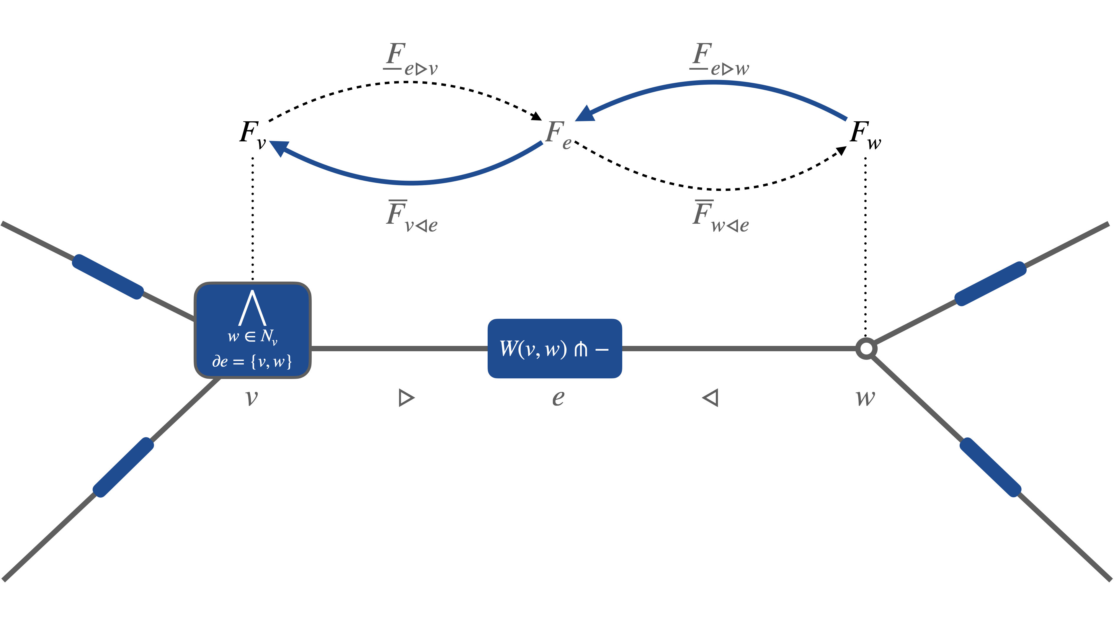
Our goal is to define an iterative process that evolves arbitrary elements of $C^{0}F$ toward fuzzy global sections using diffusion. The key tool in this construction is the Lawvere Laplacian, which operates by aggregating neighboring vertex values via weighted limits in a message-passing scheme. Passing ‘messages’ requires introducing $\mathsf{Q}$-functors $\overline{F}_{e\triangleright v}:Fe\to Fv$ that pull data back to each vertex which, when composed with $\mathsf{Q}$-functors $F_{w\triangleleft e}:Fw\to Fe$, play a role analogous to parallel transport in the connection Laplacian. Making suitable choices for these maps leads us to consider a generalized notion of adjunction suitable for approximate computations.

Definition 3.7.

For $\mathsf{Q}$-categories $\mathsf{C},\mathsf{D}$ and an element $q\in Q$, a pair of functions $F:\mathrm{ob}(\mathsf{C})\leftrightarrows\mathrm{ob}(\mathsf{D}):G$ are $q$-adjoint, written $F\dashv_{q}G$, if

$$\hom_{\mathsf{D}}(Fx,y)\approx_{q}\hom_{\mathsf{C}}(x,Gy)$$ (14)

for all $x\in\mathsf{C}$ and $y\in\mathsf{D}$. When $F$ and $G$ are additionally $\mathsf{Q}$-functors, they form an $q$-fuzzy $\mathsf{Q}$-adjunction.

This definition generalizes classical $\mathsf{Q}$-adjunctions, which we recover when $q=1$. At the other extreme, when $q=\bot$, every pair of $\mathsf{Q}$-functors forms a trivial $q$-fuzzy adjunction. The key property of $q$-adjoints is that they allow transposition of morphisms at the cost of an $q$ factor: $\hom(Fx,y)\succeq q\,\smash{\raisebox{0.80002pt}{$\scriptscriptstyle\bullet$}}\,\hom(x,Gy)$ and $\hom(x,Gy)\succeq q\,\smash{\raisebox{0.80002pt}{$\scriptscriptstyle\bullet$}}\,\hom(Fx,y)$. As we will see, this approximate adjoint structure allows the Lawvere Laplacian to identify cochains that are sufficiently close to global sections.

Proposition 3.8.

A pair of $\mathsf{Q}$-functors $F:\mathsf{C}\leftrightarrows\mathsf{D}:G$ form an $q$-fuzzy $\mathsf{Q}$-adjunction if and only if

$$\hom_{\mathsf{C}}(x,GFx)\succeq q\quad\text{ and }\quad\hom_{\mathsf{D}}(FGy,y)\succeq q$$ (15)

for all $x\in\mathsf{C}$ and $y\in\mathsf{D}$.

Proof.

Suppose $F\dashv_{q}G$ are fuzzy adjoints. Applying the contravariant Yoneda functor $[-,\hom_{\mathsf{C}}(x,GFx)]$ to the inequality $1\preceq\hom_{\mathsf{D}}(Fx,Fx)$ yields

$$[1,\hom_{\mathsf{C}}(x,GFx)]\succeq[\hom_{D}(Fx,Fx),\hom_{\mathsf{C}}(x,GFx)]\succeq q$$

where the second inequality follows from Definition 3.7. Now using the fact that $[1,p]=q$ for all $p\in Q$ we conclude $\hom_{\mathsf{C}}(x,GFx)\succeq q$. A similar argument holds for $\hom_{D}(FGy,y)$.

Conversely, suppose that $\mathsf{Q}$-functors $F$ and $G$ satisfy Eq. 15. Then, using the properties of the internal hom, we have

$\displaystyle[\hom_{\mathsf{D}}(Fx,y),\hom_{\mathsf{C}}(x,Gy)]$ $\displaystyle\succeq[\hom_{\mathsf{D}}(Fx,y),\hom_{\mathsf{C}}(x,GFx)\,\smash{\raisebox{0.80002pt}{$\scriptscriptstyle\bullet$}}\,\hom_{\mathsf{C}}(GFx,Gy)]$
$\displaystyle\succeq[\hom_{\mathsf{D}}(Fx,y),q\,\smash{\raisebox{0.80002pt}{$\scriptscriptstyle\bullet$}}\,\hom_{\mathsf{C}}(GFx,Gy)]$
$\displaystyle\succeq q\,\smash{\raisebox{0.80002pt}{$\scriptscriptstyle\bullet$}}\,[\hom_{\mathsf{D}}(Fx,y),\hom_{\mathsf{C}}(GFx,Gy)]$
$\displaystyle\succeq q\,\smash{\raisebox{0.80002pt}{$\scriptscriptstyle\bullet$}}\,[\hom_{\mathsf{D}}(Fx,y),\hom_{\mathsf{C}}(Fx,y)]$
$\displaystyle\succeq q\,\smash{\raisebox{0.80002pt}{$\scriptscriptstyle\bullet$}}\,1=q$

where we use Lemma 2.1 for the second, third and fourth inequality. The reverse fuzzy inequality follows from a similar argument. ∎

We consider an example of a crisp and fuzzy $\mathsf{Q}$-adjunction encountered in applications (see Section 4.1).

Example 3.9.

Suppose $\mathsf{C}$ and $\mathsf{D}$ are discrete $\mathsf{R}$-categories with objects $\mathrm{ob}(\mathsf{C})=\{1,2,\dots,m\}$, $\mathrm{ob}(\mathsf{D})=\{1,2,\dots,n\}$. For convenience, we write $z_{+}$ for $\max\{z,0\}$, so the $\mathsf{R}$-category $\widehat{C}^{\mathrm{op}}:=[\mathsf{C}^{\mathrm{op}},\underline{\mathsf{R}}]^{\mathrm{op}}$ has $\hom_{\widehat{\mathsf{C}}^{\mathrm{op}}}(x,y)=\max_{i\in\mathsf{C}}\bigl{(}x(i)-y(i)\bigr{)}_{+}$. Given an $m\times n$ $\mathsf{R}$-valued matrix $A$, we obtain an $\mathsf{R}$-functor $F:\widehat{\mathsf{C}}^{\mathrm{op}}\to\widehat{\mathsf{D}}^{\mathrm{op}}$ analogous to matrix-vector multiplication $Fx(j)=\max_{i\in\mathsf{C}}\left\{x(i)+A(i,j)\right\}$. It follows that $F$ is an $\mathsf{R}$-functor since

$\displaystyle\begin{aligned} \hom_{\widehat{\mathsf{D}}^{\mathrm{op}}}(Fx,Fy)&=\max_{j\in\mathsf{D}}\Bigl{(}\max_{i\in\mathsf{C}}\left\{x(i)+A(i,j)\right\}-\max_{i\in\mathsf{C}}\left\{y(i)+A(i,j)\right\}\Bigr{)}_{+}\\ &\leq\max_{i\in\mathsf{C}}\bigl{(}x(i)-y(i)\bigr{)}_{+}\\ &=\hom_{\widehat{\mathsf{C}}^{\mathrm{op}}}(x,y)\end{aligned}$ (16)

We may also obtain the transpose $\mathsf{R}$-functor $G:\widehat{\mathsf{D}}^{\mathrm{op}}\to\widehat{\mathsf{C}}^{\mathrm{op}}$ defined by $Gy(i)=\min_{j\in\mathsf{D}}\bigl{(}y(j)-A(i,j)\bigr{)}_{+}$, which is an $\mathsf{R}$-functor by a similar argument. Indeed we have

$\displaystyle\hom_{\widehat{\mathsf{D}}^{\mathrm{op}}}\bigl{(}Fx,y\bigr{)}$ $\displaystyle=\max_{j\in\mathsf{D}}\Bigl{(}\max_{i\in\mathsf{C}}\bigl{\{}x(i)+A(i,j)\bigl{\}}-y(j)\Bigr{)}_{+}$
$\displaystyle=\max_{i\in\mathsf{C}}\Bigl{(}x(i)-\min_{j\in\mathsf{D}}\bigl{(}y(j)-A(i,j)\bigr{)}_{+}\Bigr{)}_{+}$
$\displaystyle=\hom_{\widehat{\mathsf{C}}^{\mathrm{op}}}\bigl{(}x,Gy\bigr{)}$

so we can conclude $F\dashv_{0}G$. We now consider a fuzzy version of the above adjunction. Suppose $\tilde{F}x(j)=\max_{i\in\mathsf{C}}\left\{x(i)+A(i,j)+\eta_{i}\right\}$ where $\eta_{i}\sim\mathrm{Unif}([0,q])$ is a uniform random variable. Observe $(\eta-\eta^{\prime})_{+}\leq q$ whenever $\eta,\eta^{\prime}\sim\mathrm{Unif}([0,q])$ and that $F\approx_{q}\tilde{F}$ follows from Eq. 16. Finally, it follows that $\tilde{F}\dashv_{q}G$ by applying Proposition A.5.

The above definitions lead to a sheaf Laplacian which we call the Lawvere Laplacian. Later, we will show that this Laplacian permits recursive computation of global sections.

Definition 3.10.

Consider a network sheaf $\underline{F}:\mathcal{G}^{\mathrm{op}}\to\mathsf{Q}\mathsf{C}\mathsf{Cat}$ on a graph $G=(V,E)$ and a network cosheaf $\overline{F}:\mathcal{G}\to\mathsf{Q}\mathsf{C}\mathsf{Cat}$ which agree on objects; for an object $\sigma\in V\sqcup E$, we write $F\sigma:=\underline{F}\sigma=\overline{F}\sigma$. We define the Lawvere Laplacian of $F$ weighted by $W$ to be the function $L_{W}:\mathrm{ob}(C^{0}F)\to\mathrm{ob}(C^{0}F)$ taking an object $\vec{x}=(x_{v})_{v\in V}$ to the object whose $v$-th coordinate is given by the following weighted meet

$\displaystyle\left(L_{W}\vec{x}\right)_{v}:=\bigwedge_{\begin{subarray}{c}w\in N_{v}\\ \partial e=\{v,w\}\end{subarray}}^{W(v,-)}\overline{F}_{e\triangleright v}\underline{F}_{w\triangleleft e}x_{w}.$ (17)

We say $L_{W}$ is $q$-fuzzy if for every incidence $v\triangleleft e$ we have that $\underline{F}_{v\triangleleft e}\dashv_{q}\overline{F}_{e\triangleright v}$. We say $L_{W}$ is crisp when $L_{W}$ is $1$-fuzzy.

Remark 3.11.

For every $v\triangleleft e\triangleright w$, the composition $\overline{F}_{e\triangleright v}\underline{F}_{w\triangleleft e}:Fw\to Fv$ is analogous to parallel transport (see Section 1.1.5). To understand the explicit action of the Lawvere Laplacian on 0-chains, we apply Theorem 2.11 to obtain

$\displaystyle\left(L_{W}\vec{x}\right)_{v}\approx_{1}\bigwedge_{\begin{subarray}{c}w\in N_{v}\\ \partial e=\{v,w\}\end{subarray}}W(v,w)\,\pitchfork\,\overline{F}_{e\triangleright v}\underline{F}_{w\triangleleft e}x_{w}.$ (18)

Compare this with the (random walk) graph connection Laplacian

$\displaystyle(L\vec{x})_{v}=\sum_{w\in N_{v}}W(v,w)\cdot O_{v}^{\top}O_{w}x_{w}$ (19)

where $\vec{x}\in\textstyle\bigoplus_{v\in V}\mathbb{R}^{d}$ and the matrix product $O_{v}^{\top}O_{w}$ induces an orthogonal map $\mathbb{R}^{d}\to\mathbb{R}^{d}$ approximating parallel transport. Thus, the Lawvere Laplacian integrates objects in a manner similar to the graph connection Laplacian, modulating the aggregation of objects according to a weight function.

Remark 3.12.

Note that the stalks of the network sheaf $F$ may not be skeletal and hence the Lawvere Laplacian is defined only up to isomorphism. Therefore, as a computational tool, one should pass to the skeleton of each stalk to obtain a well-defined function. In general, for non-skeletal stalks, we can make arbitrary choices of isomorphism classes to obtain an honest function.

Refer to caption
Figure 1: The Lawvere Laplacian

In order to apply the Enriched Tarski Fixed Point Theorem (Theorem 2.17), we demonstrate the functoriality of the Lawvere Laplacian by showing

$\displaystyle\hom_{C^{0}F}(\vec{x},\vec{y})\preceq\hom_{C^{0}F}(L_{W}\vec{x},L_{W}\vec{y}),\quad\forall\vec{x},\vec{y}\in C^{0}F.$
Lemma 3.13.

The Lawvere Laplacian $L_{W}$ is a $\mathsf{Q}$-functor.

Proof.

For each $v\in V$ and $v\triangleleft e\triangleright w$, we have that

$$\hom_{Fw}(x_{w},y_{w})\preceq\hom_{Fv}(\overline{F}_{e\triangleright v}\underline{F}_{w\triangleleft e}x_{w},\overline{F}_{e\triangleright v}\underline{F}_{w\triangleleft e}y_{w})$$

by the functoriality of $\overline{F}_{e\triangleright v}\underline{F}_{w\triangleleft e}$. Thus, with $v$ fixed

$\displaystyle\bigwedge_{\begin{subarray}{c}w\in N_{v}\\ \partial e=\{v,w\}\end{subarray}}\hom_{Fw}(x_{w},y_{w})$ $\displaystyle\preceq\bigwedge_{\begin{subarray}{c}w\in N_{v}\\ \partial e=\{v,w\}\end{subarray}}\hom_{Fv}(\overline{F}_{e\triangleright v}\underline{F}_{w\triangleleft e}x_{w},\overline{F}_{e\triangleright v}\underline{F}_{w\triangleleft e}y_{w})$
$\displaystyle\preceq\hom_{Fv}\left(\bigwedge^{W(v,-)}_{\begin{subarray}{c}w\in N_{v}\\ \partial e=\{v,w\}\end{subarray}}\overline{F}_{e\triangleright v}\underline{F}_{w\triangleleft e}x_{w},\bigwedge^{W(v,-)}_{\begin{subarray}{c}w\in N_{v}\\ \partial e=\{v,w\}\end{subarray}}\overline{F}_{e\triangleright v}\underline{F}_{w\triangleleft e}y_{w}\right)$

where the second inequality comes from Lemma A.2. Now quantifying over $v$, we find that

$\displaystyle\bigwedge_{v\in V}\hom_{Fv}(x_{v},y_{v})$ $\displaystyle\preceq\bigwedge_{v\in V}\bigwedge_{\begin{subarray}{c}w\in N_{v}\\ \partial e=\{v,w\}\end{subarray}}\hom_{Fw}(x_{w},y_{w})$
$\displaystyle\preceq\bigwedge_{v\in V}\hom_{Fv}\left(\bigwedge^{W(v,-)}_{\begin{subarray}{c}w\in N_{v}\\ \partial e=\{v,w\}\end{subarray}}\overline{F}_{e\triangleright v}\underline{F}_{w\triangleleft e}x_{w},\bigwedge^{W(v,-)}_{\begin{subarray}{c}w\in N_{v}\\ \partial e=\{v,w\}\end{subarray}}\overline{F}_{e\triangleright v}\underline{F}_{w\triangleleft e}y_{w}\right).$

The Lawvere Laplacian $L_{W}$ captures the $W$-fuzzy global sections of the associated network sheaf according to following lemmas.

Lemma 3.14.

Suppose $L_{W}$ is an $\varepsilon$-fuzzy Lawvere Laplacian. For a 0-cochain $\vec{x}\in C^{0}F$, if

$$\hom_{Fe}(\underline{F}_{v\triangleleft e}x_{v},\underline{F}_{w\triangleleft e}x_{w})\succeq W(v,w)\,\smash{\raisebox{0.80002pt}{$\scriptscriptstyle\bullet$}}\,q$$ (20)

for all edges $e$ such that $v\triangleleft e\triangleright w$, then $\vec{x}\in\mathcal{S}_{\varepsilon\,\smash{\raisebox{0.56001pt}{$\scriptscriptstyle\bullet$}}\,q}(L_{W})$.

Proof.

We would like to show $\hom_{C^{0}F}\left(\vec{x},L_{W}\vec{x}\right)\succeq\varepsilon\,\smash{\raisebox{0.80002pt}{$\scriptscriptstyle\bullet$}}\,q$. We may write that

$\displaystyle\hom_{C^{0}F}\left(\vec{x},L_{W}\vec{x}\right)$ $\displaystyle=\bigwedge_{v\in V}\hom_{Fv}\bigg{(}x_{v},\bigwedge_{\begin{subarray}{c}w\in N_{v}\\ \partial e=\{v,w\}\end{subarray}}^{W}\overline{F}_{e\triangleright v}\underline{F}_{w\triangleleft e}x_{w}\bigg{)}$
$\displaystyle=\bigwedge_{v\in V}\bigwedge_{\begin{subarray}{c}w\in N_{v}\\ \partial e=\{v,w\}\end{subarray}}[W(v,w),\hom_{Fv}(x_{v},\overline{F}_{e\triangleright v}\underline{F}_{w\triangleleft e}x_{w})]$

and hence we equivalently show that for all $e$ such that $v\triangleleft e\triangleright w$

$\displaystyle\left[W(v,w),\hom_{Fv}(x_{v},\overline{F}_{e\triangleright v}\underline{F}_{w\triangleleft e}x_{w})\right]\succeq\varepsilon\,\smash{\raisebox{0.80002pt}{$\scriptscriptstyle\bullet$}}\,q$

which holds if and only if

$\displaystyle\hom_{Fv}(x_{v},\overline{F}_{e\triangleright v}\underline{F}_{w\triangleleft e}x_{w})\succeq W(v,w)\,\smash{\raisebox{0.80002pt}{$\scriptscriptstyle\bullet$}}\,\varepsilon\,\smash{\raisebox{0.80002pt}{$\scriptscriptstyle\bullet$}}\,q.$ (21)

Now observe that Eq. 21 holds because $\varepsilon$-fuzziness of $L_{W}$ implies

$\displaystyle[\hom_{Fv}(x_{v},\overline{F}_{e\triangleright v}\underline{F}_{w\triangleleft e}x_{w}),\hom_{Fe}(\underline{F}_{v\triangleleft e}x_{v},\underline{F}_{w\triangleleft e}x_{w})]\succeq\varepsilon$

which implies

$\displaystyle\hom_{Fv}(x_{v},\overline{F}_{e\triangleright v}\underline{F}_{w\triangleleft e}x_{w})\succeq\varepsilon\,\smash{\raisebox{0.80002pt}{$\scriptscriptstyle\bullet$}}\,\hom_{Fe}(\underline{F}_{v\triangleleft e}x_{v},\underline{F}_{w\triangleleft e}x_{w})\succeq W(v,w)\,\smash{\raisebox{0.80002pt}{$\scriptscriptstyle\bullet$}}\,\varepsilon\,\smash{\raisebox{0.80002pt}{$\scriptscriptstyle\bullet$}}\,q.$

Lemma 3.15.

If $\vec{x}\in\mathcal{S}_{q}(L_{W})$ then for all edges $e$ such that $v\triangleleft e\triangleright w$

$$\hom_{Fe}(\underline{F}_{v\triangleleft e}x_{v},\underline{F}_{w\triangleleft e}x_{w})\succeq W(v,w)\,\smash{\raisebox{0.80002pt}{$\scriptscriptstyle\bullet$}}\,\varepsilon\,\smash{\raisebox{0.80002pt}{$\scriptscriptstyle\bullet$}}\,q.$$ (22)
Proof.

If $\vec{x}\in\mathcal{S}_{q}(L_{W})$, then from the argument above we may deduce

$\displaystyle\hom_{Fv}(x_{v},\overline{F}_{e\triangleright v}\underline{F}_{w\triangleleft e}x_{w})\succeq W(v,w)\,\smash{\raisebox{0.80002pt}{$\scriptscriptstyle\bullet$}}\,q$

for all edges $e$ such that $v\triangleleft e\triangleright w$. It follows that

$\displaystyle\hom_{Fv}(\underline{F}_{v\triangleleft e}x_{v},\underline{F}_{w\triangleleft e}x_{w})\succeq\varepsilon\,\smash{\raisebox{0.80002pt}{$\scriptscriptstyle\bullet$}}\,\hom_{Fv}(x_{v},\overline{F}_{e\triangleright v}\underline{F}_{w\triangleleft e}x_{w})\succeq W(v,w)\,\smash{\raisebox{0.80002pt}{$\scriptscriptstyle\bullet$}}\,\varepsilon\,\smash{\raisebox{0.80002pt}{$\scriptscriptstyle\bullet$}}\,q.$

Lemma 3.14 and Lemma 3.15 are not converese to each other. However, when $\varepsilon$ is idempotent, we obtain the following lemma.

Lemma 3.16.

Suppose $\varepsilon\in Q$ is idempotent. Then $\vec{x}\in\mathcal{S}_{\varepsilon\,\smash{\raisebox{0.56001pt}{$\scriptscriptstyle\bullet$}}\,q}(L_{W})$ if and only if

$$\hom_{Fe}(\underline{F}_{v\triangleleft e}x_{v},\underline{F}_{w\triangleleft e}x_{w})\succeq W(v,w)\,\smash{\raisebox{0.80002pt}{$\scriptscriptstyle\bullet$}}\,\varepsilon\,\smash{\raisebox{0.80002pt}{$\scriptscriptstyle\bullet$}}\,q.$$
Proof.

Suppose $\vec{x}\in\mathcal{S}_{\varepsilon\,\smash{\raisebox{0.56001pt}{$\scriptscriptstyle\bullet$}}\,q}(L_{W})$, then Lemma 3.15 implies

$$\hom_{Fe}(\underline{F}_{v\triangleleft e}x_{v},\underline{F}_{w\triangleleft e}x_{w})\succeq W(v,w)\,\smash{\raisebox{0.80002pt}{$\scriptscriptstyle\bullet$}}\,\varepsilon^{2}\,\smash{\raisebox{0.80002pt}{$\scriptscriptstyle\bullet$}}\,q=W(v,w)\,\smash{\raisebox{0.80002pt}{$\scriptscriptstyle\bullet$}}\,\varepsilon\,\smash{\raisebox{0.80002pt}{$\scriptscriptstyle\bullet$}}\,q.$$

The converse directly follows from Lemma 3.14 because the above equation implies $\vec{x}\in\mathcal{S}_{\varepsilon^{2}\,\smash{\raisebox{0.56001pt}{$\scriptscriptstyle\bullet$}}\,q}(L_{W})=\mathcal{S}_{\varepsilon\,\smash{\raisebox{0.56001pt}{$\scriptscriptstyle\bullet$}}\,q}(L_{W})$. ∎

The preceding lemmas imply there is an isomorphim between the $\mathsf{Q}$-category of suffix points and the $\mathsf{Q}$-category of $W$-fuzzy global sections when $L_{W}$ is crisp.

Theorem 3.17.

If $L_{W}$ is a crisp Lawvere Laplacian, then there is an isomorphism $\mathcal{S}(L_{W})\cong\Gamma_{W}F$ of $\mathsf{Q}$-categories.

Proof.

Idempotence of the identity together with Lemma 3.16 imply $\hom_{C^{0}}(\vec{x},L_{W}(\vec{x}))=1$ if and only if

$\displaystyle\hom_{Fe}(\underline{F}_{v\triangleleft e}x_{v},\underline{F}_{w\triangleleft e}x_{w})\succeq W(v,w)$

for all $e$ such that $v\triangleleft e\triangleright w$, that is, $\vec{x}\in\Gamma_{W}F$ according to Theorem 3.6. Hence, the isomorphism between $\mathcal{S}(L_{W})$ and $\Gamma_{W}F$ is the identity on objects. It suffices, then, to show that

$\displaystyle\hom_{\mathcal{S}(L_{W})}(\vec{x},\vec{y})=\hom_{\Gamma_{W}F}(\vec{x},\vec{y}).$

which also follows from Theorem 3.6. ∎

Theorem 3.17 is analogous to the Hodge Theorem [15] which states that the harmonic cochains are isomorphic to cohomology. Here, we interpret $\mathcal{S}(L_{W})$ as the harmonic cochains and $\Gamma_{W}F$ as cohomology.

3.3 Harmonic Flow

To bridge the gap between a fixed-point description of global sections and an algorithm to compute global sections, we introduce a notion of a flow.

Definition 3.18.

The flow functor $\Phi_{W}^{\omega}=\Phi:C^{0}F\to C^{0}F$ is the $\mathsf{Q}$-functor

$$\left(\Phi\vec{x}\right)_{v}:=\left(L_{W}\vec{x}\right)_{v}\prescript{\omega_{1}(v)}{}{\wedge}^{\omega_{2}(v)}x_{v}.$$

where $\omega_{i}:V\to\mathsf{Q}$ are flow weightings. Iterating $\Phi$ with an initial condition $\vec{x}[0]=\vec{x}_{0}\in C^{0}F$ results in the harmonic flow

$$\vec{x}[t+1]=\Phi(\vec{x}[t]).$$

We say the harmonic flow is unweighted when $\omega_{1}=\omega_{2}=1$.

Asynchronous or adaptive updates, for instance, can be captured by assigning appropriate flow weightings, possibly changing each iteration. An example is considered in Section 4.2. For the remainder of this section, we focus on unweighted harmonic flow under which the fixed points of the flow functor are exactly the suffix points of $L_{W}$. Moreover, since $L_{W}$ is a $\mathsf{Q}$-endofunctor we can apply Theorem 2.17 to conclude the following.

Corollary 3.19.

The suffix points of the Lawvere Laplacian $\mathcal{S}(L_{W})$ form a weighted lattice.

When the unweighted harmonic flow converges in finitely many iterations, the following monotonicity property (see Section 1.1.3) is observed.

Proposition 3.20.

Suppose $L_{W}$ is a crisp Lawvere Laplacian. If the unweighted harmonic flow converges in finitely many iterations to $\vec{x}[\infty]$ then for all $\vec{y}\in\Gamma_{W}F$ we have

$$\hom_{C^{0}F}(\vec{y},\vec{x}[0])=\hom_{C^{0}F}(\vec{y},\vec{x}[\infty]).$$
Proof.

First observe that if $\vec{x}[t]\succeq_{1}\vec{y}$ and $\vec{y}\in\Gamma_{W}F$ then, because $L_{W}(\vec{x}[t])\succeq_{1}L_{W}(\vec{y})\succeq_{1}\vec{y}$ by Theorem 3.17, we have

$$\vec{x}[t+1]=\vec{x}[t]\wedge L_{W}(\vec{x}[t])\succeq_{1}\vec{y}.$$

Hence the harmonic flow must converge to an object

$$\vec{x}[\infty]\cong\bigvee\{\vec{z}\in\Gamma_{W}F\mid\vec{z}\preceq_{1}\vec{x}[0]\}$$

which is equivalent to the weighted join

$$\vec{x}[\infty]\cong\bigvee_{\vec{z}\in\Gamma_{W}F}\hom(\vec{z},\vec{x}[0])\otimes\vec{z}.$$

Now observe that $\hom_{C^{0}F}(\vec{y},\vec{x}[\infty])\preceq\hom_{C^{0}F}(\vec{y},\vec{x}[0])$ follows from Lemma 2.1 and that

$\displaystyle\hom(\vec{y},\vec{x}[\infty])$ $\displaystyle=\hom\bigg{(}\vec{y},\bigvee_{\vec{z}\in\Gamma(F,W)}\hom(\vec{z},\vec{x}[0])\otimes\vec{z}\bigg{)}$
$\displaystyle\succeq\hom(\vec{y},\hom(\vec{y},\vec{x}[0])\otimes\vec{y})$
$\displaystyle\succeq\hom(\vec{y},\vec{y})\,\smash{\raisebox{0.80002pt}{$\scriptscriptstyle\bullet$}}\,\hom(\vec{y},\vec{x}[0])$
$\displaystyle=\hom(\vec{y},\vec{x}[0])$

where we again used Lemma 2.1 and Lemma A.4. ∎

Remark 3.21.

There is a sense in which 3.20 is analogous to the fact that for a sheaf of (finite dimensional) vector spaces, the heat equation (1) with initial condition $\vec{x}_{0}$ converges to its orthogonal projection onto the space global sections (cf. [22]). In particular, an orthogonal projection $P:V\to V$ onto a vector subspace $W\subseteq V$ preserves the inner product $\langle w,Pv\rangle=\langle w,v\rangle$ for all $w\in W$. Note, however, that $\hom_{C^{0}F}(\vec{x}[0],\vec{y})=\hom_{C^{0}F}(\vec{x}[\infty],\vec{y})$ may not necessarily hold.

In the absence of finiteness conditions on each stalk, such as convergence of descending chains, it is not guaranteed that the unweighted harmonic flow converges to a fixed point in finitely many iterations. Consider a simple counterexample.

Example 3.22.

Without finiteness conditions, it is easy to construct Laplacians which do not reach a fixed point in finitely many iterations of the harmonic flow (although, in the $\mathsf{B}$-enriched setting, [10] show that fixed points are reached after a transfinite number of iterations). For example, consider the complete graph on three vertices $G=(V,E)$ with $V=\{1,2,3\}$. Define the sheaf $F$ to have all stalks given by $F(\sigma)\cong\underline{\mathsf{R}}$ and restriction maps $F_{v\triangleleft\{v,w\}}=\mathrm{id}$ for $v=w+1\,(\text{mod }3)$ and $F_{v\triangleleft\{v,w\}}(x)=x+1$ for all other incidences. One can check that the unweighted harmonic flow of the unweighted crisp Lawvere Laplacian initialized at $\vec{x}_{0}=(0,0,0)$ does not converge in finitely iterations. Indeed the only global section of this sheaf is $(\infty,\infty,\infty)$.

4 Applications

In this section we outline some initial uses of the Lawvere Laplacian.

4.1 Synchronization of Discrete Event Systems

Quantales and $\mathsf{Q}$-categories, often described as idempotent semi-rings and semi-modules, are fundamental in certain models of discrete event systems. These are systems in which state changes triggered by the occurrence of specific events take place at discrete points in time. In general, discrete event systems are notoriously difficult to model, but an important class of these systems exhibiting linear-like structure [13, 8] can be described in the framework of $\mathsf{Q}$-categories.

Suppose $\mathsf{C}$ is a discrete category with objects $\mathrm{ob}(\mathsf{C})=\{1,2,\dots,m\}$ indexing particular events. In our language, a discrete-time linear system can be described by the recursion $x[t+1]=T(x[t])$ where $T$ is a $\mathsf{R}$-functor $T:\widehat{\mathsf{C}}^{\mathrm{op}}\to\widehat{\mathsf{C}}^{\mathrm{op}}$ preserving weighted joins and where where $x[t]\in\widehat{\mathsf{C}}^{\mathrm{op}}$ is interpreted as a vector of timings for events after $t$ occurrences. A generic form (see Example 3.9) for such a functor is given by

$\displaystyle T(x)=\bigl{(}\max_{i\in\mathsf{C}}\{x(i)+A(i,j)\}\bigr{)}_{j\in\mathsf{C}}$ (23)

where $A$ is a $m\times m$ $\mathsf{R}$-valued matrix interpreted as delays between events. The synchronization problem for two discrete event systems is to determine time assignments for each system such that future occurrences of events are synchronized between the two systems [11].

In this example, we utilize the Lawvere Laplacian to simultaneously solve an approximate network synchronization problem. Let $G=(V,E)$ be a graph where vertices $V=\{1,2,\dots,n\}$ index discrete event systems (e.g. production cells) which interact as subsystems of a larger complex system. Pairwise interactions between systems are modeled by edges in a graph. Let $F$ be a network sheaf on $G$ with stalks $F(\sigma)=\widehat{\mathsf{C}}^{\mathrm{op}}$. Now $W$-fuzzy global sections correspond to synchronous time assignments and the restriction maps of $\underline{F}$ have the form Eq. 23. We define a network cosheaf $\overline{F}$ so that $\underline{F}_{e\triangleleft v}\dashv\overline{F}_{v\triangleleft e}$ forms a crisp $\mathsf{R}$-adjunction (see Example 3.9). The relations, and thus the delays between events, vary from node to node. A graph weighting $W:V\times V\to\mathsf{R}$ describes synchronization constraints between systems. For instance, if two coupled systems $v$ and $w$ must be fully synchronized, then $W(v,w)=0$, while $W(v,w)=\infty$ for unsynchronized systems. A $W$-fuzzy global section is a timing assignment $(x_{v})_{v\in V}$ for all systems and for all events such that events between coupled systems are synchronized up to $W$, that is,

$\displaystyle\begin{aligned} \min_{j\in\mathsf{C}}\Bigl{(}\max_{i\in\mathsf{C}}\{x_{w}(i)+A_{w}(i,j)\}-\max_{i\in\mathsf{C}}\{x_{v}(i)+A_{v}(i,j)\}\Bigr{)}_{+}\leq W(v,w)\\ \min_{j\in\mathsf{C}}\Bigl{(}\max_{i\in\mathsf{C}}\{x_{v}(i)+A_{v}(i,j)\}-\max_{i\in\mathsf{C}}\{x_{w}(i)+A_{w}(i,j)\}\Bigr{)}_{+}\leq W(w,v)\\ \end{aligned}\quad\forall\{v,w\}\in E$ (24)

In a $W$-fuzzy global section, events are seperated by at most $W(u,v)$ or $W(v,w)$ time units for every edge $\{u,v\}\in E$. Because the cotensor in $\widehat{\mathsf{C}}^{\mathrm{op}}$ is given by $(a\pitchfork x)(i)=a+x(i)$, the Lawvere Laplacian is then given by the following

$\displaystyle(L_{W}\vec{x})_{v}$ $\displaystyle=\biggl{(}\min_{\begin{subarray}{c}w\in N_{v}\\ \partial e=\{v,w\}\end{subarray}}W(v,w)+\min_{j\in\mathsf{C}}\Bigl{\{}\Bigr{(}A_{v}(i^{\prime},j)-\max_{i\in\mathsf{C}}\{A_{w}(i,j)+x_{w}(i)\}\Bigr{)}_{+}\Bigr{\}}\biggr{)}_{i^{\prime}\in\mathsf{C}}.$ (25)

It follows by Theorem 3.17 that $\mathcal{S}(L_{W})$ are the $W$-fuzzy global sections, i.e. the solutions of Eq. 24.

4.2 Shortest-Path Problems

It has also been shown [2, 31] that quantales can be used to solve various path problems in networks, which has led to, for example, generalized shortest-path algorithms such as Bellman-Ford, Dijkstra, and Floyd-Marshall. The Lawvere Laplacian can provide a framework for describing and proving formal properties of these algorithms in the presence of ’fuzziness’ or inexact computation. As a simple example, we consider the problem of computing the smallest weight path in a graph with Djikstra’s algorithm.

Let $G=(V,E)$ be an undirected graph with an edge weighting $W:E\to\mathsf{R}$ and vertices $V=\{1,2,\dots,n\}$ with a distinguished source node $s=1$ and target node $t=n$. Let $F$ be the constant network sheaf on $\mathcal{G}$ with stalks $F(\sigma)=\underline{\mathsf{R}}^{\mathrm{op}}$. Note that in $\underline{\mathsf{R}}^{\mathrm{op}}$ meets and cotensors are equivalent to joins and tensors in $\underline{\mathsf{R}}$. Hence in $\underline{\mathsf{R}}^{\mathrm{op}}$, $x\wedge y=\min\{x,y\}$ and $\alpha\pitchfork x=\alpha+x$. The edge weights $W$ are equivalent to a symmetric graph weighting $W:V\times V\to\mathsf{R}$. The Lawvere Laplacian is

$\displaystyle(L_{W}\vec{x})_{v}=\min_{w\in N_{v}}\{W(v,w)+x_{w}\}.$

and harmonic flow is given by applying a flow functor

$\displaystyle\left(\Phi\vec{x}\right)_{v}$ $\displaystyle:=\left(L_{W}\vec{x}\right)_{v}\prescript{\omega_{1}(v)}{}{\wedge}^{\omega_{2}(v)}x_{v}$
$\displaystyle=\min\bigl{\{}\omega_{1}(v)+\min_{w\in N_{v}}\{W(v,w)+x_{w}\},x_{v}+\omega_{2}(w)\bigr{\}}$

To recover Djikstra’s algorithm, set $\omega_{2}(v)=0$ and

$$\omega_{1}(v;U)=\begin{cases}0,&v\in U\\ \infty,&\text{else}\end{cases}$$

where $U\subseteq V$ is a subset acting as a pointer to which nodes have not previously been searched. This serves as an example of harmonic flow where flow weights are are continually updated as $U$ is updated each round of Djikstra.

4.3 Preference Diffusion

In this section, we give an application of categorical diffusion to preference dynamics, which can model, for example, changes in opinions held by agents (e.g. consumers, voters) on the relative ordering of alternatives (e.g. candidates, products resp.). Recall that a preference relation is simply an $\mathsf{I}$-category.

Proposition 4.1.

The set $\mathsf{Pref}(A)$ of $\mathsf{Q}$-valued preference relations on $A$ with

$$\hom_{\mathsf{Pref}(A)}(P,M):=\bigwedge_{a,b\in A}[P(a,b),M(a,b)]$$

is a weighted lattice.

Proof.

Observe that for any preference relation $P$, the assignment

$$(q\pitchfork P)(a,b):=[q,P(a,b)]$$

is a preference relation. This operation is easily shown to be the cotensor on $\mathsf{Pref}(A)$ using Lemma 2.1. Moreover, it is easy to check that the crisp meets are given by

$$(P\wedge M)(a,b)=P(a,b)\wedge M(a,b)$$

which is a preference relation since, by the affineness of $\mathsf{Q}$, we have

$$(P\wedge M)(a,c)\succeq(P\wedge M)(a,b)\,\smash{\raisebox{0.80002pt}{$\scriptscriptstyle\bullet$}}\,(P\wedge M)(b,c).$$

By virtue of admitting all weighted meets, we can conclude $\mathsf{Pref}(A)$ admits all weighted joins by Lemma 2.9. Explicitly, we have that

$\displaystyle(P\vee M)(a,b)$ $\displaystyle=\bigvee_{x\in A}\big{(}P(a,x)\vee M(a,x)\big{)}\,\smash{\raisebox{0.80002pt}{$\scriptscriptstyle\bullet$}}\,\big{(}P(x,b)\vee M(x,b)\big{)}$
$\displaystyle(q\otimes P)(a,b)$ $\displaystyle=\big{(}q\,\smash{\raisebox{0.80002pt}{$\scriptscriptstyle\bullet$}}\,P(a,b)\big{)}\vee 1(a,b)$

where $1\in\mathsf{Pref}(A)$ is the discrete preference relation. ∎

Given a set function $f:A\to B$ we obtain an induced crisp adjunction $f_{\ast}\dashv f^{\ast}:\mathsf{Pref}(A)\to\mathsf{Pref}(B)$ where the right adjoint is

$$f^{\ast}M(a,a^{\prime}):=M(f(a),f(a^{\prime}))$$

for $M\in\mathsf{Pref}(B)$. Since $f^{\ast}$ preserves weighted meets, it must have a left adjoint $f_{\ast}$ and by Remark A.8 it is given by the crisp meet

$$f_{\ast}P=\bigwedge\{M\in\mathsf{Pref}(B)\mid f^{\ast}M\succeq_{1}P\}.$$

Given a network sheaf of sets $F:\mathcal{G}^{\mathrm{op}}\to\mathsf{Set}$ we can naturally obtain a sheaf of preference relations $\mathsf{Pref}(F):\mathcal{G}^{\mathrm{op}}\to\mathsf{Q}\mathsf{C}\mathsf{Cat}$ by defining $\mathsf{Pref}(F)(\sigma):=\mathsf{Pref}(F\sigma)$ with restriction maps given by the induced left adjoints $\mathsf{Pref}(F_{v\triangleleft e}):=(F_{v\triangleleft e})_{\ast}$.

Example 4.2 (Bounded Confidence).

The Hegselmann-Krause model of bounded confidence [24] is naturally expressed using programmable weights $W$. We can make the graph weights dependent on the distance between neighboring agents’ preferences, explicitly, we let $W(-;v,w):Fv\times Fw\to\mathsf{Q}$ determine the strength of influence vertex $v$ has on $w$ based on their respective preference relations $x_{v}$ and $x_{w}$:

$$W(x_{v},x_{w};v,w)=\begin{cases}1,&x_{v}\approx_{\varepsilon_{v}}x_{w}\\ \bot,&\text{otherwise}\end{cases}$$

where $\varepsilon_{v}\in Q$ is a vertex-specific confidence threshold. This formulation ensures that agents are only influenced by neighbors whose preferences lie within their confidence bounds, as measured by the $\varepsilon_{v}$-approximate equality relation.

5 Conclusion

The Lawvere Laplacian developed herein provides a categorical formalization of diffusion processes in which exact consistency between neighboring values may be neither achievable nor necessary. Through $\varepsilon$-fuzzy adjunctions between enriched categories, this framework naturally accommodates approximate parallel transport, enabling precise quantification of information degradation across network morphisms. Aggregating transported ’tangent vectors’ via weighted meets, the Lawvere Laplacaian strongly resembles the connection Laplacain. This represents a fundamental advancement over existing frameworks predicated on exact adjunctions or strict coherence. Our primary theoretical contribution extends both Tarski’s fixed point theory and graph Laplacian diffusion, establishing that both prefix and suffix points of the Lawvere Laplacian form complete categories. The resulting harmonic flow, constructed via fuzzy adjoint pairs, provides an explicit method for computing $W$-fuzzy global sections, unifying discrete-time diffusion processes with weighted limits in enriched category theory.

Several promising theoretical directions remain for future investigation:

  • The Tarski Fixed Point Theorem and specific results for network sheaves can likely be lifted to a larger class of enrichment bases such as quantaloid-enriched categories [37, 39]. Note that in these cases, when the enriching base is neither commutative nor affine, our interpretations of ‘fuzziness’ may not be well-suited.

  • The Lawvere Laplacian is defined over a preorder modeling an undirected graph. We would like to expand the scope to include enriched categories modeling arbitrary base spaces, including simplicial sets.

  • A limitation of the Lawvere Laplacian construction is that it does not directly generalize established approaches. For instance, the Lawvere Laplacian cannot recover the graph connection Laplacian for an appropriate choice of enriching category. Instead, we rely on the analogy between adjoint $\mathsf{Q}$-functors and adjoint linear operators. To extend the scope of the Lawvere Laplacian, one approach is to consider monoidal structures on $\mathsf{Q}$-categories other than the monoidal structure given by the crisp meet. Our completeness results can likely be extended if the monoidal structure exhibits an appropriate universal property. Another avenue is the Chu construction [3], which lifts both the concepts of adjoint operators and adjoint functors.

  • We introduced fuzzy functors and adjunctions in enriched category theory and suspect we have only scratched the surface of their applicability. Fuzzy or approximate versions of standard theorems are abound in the spirit of, for example, our fuzzy Yoneda Lemma A.3. More complicated bases of enrichment may also provide a wealth of interesting examples and applications.

  • Recent efforts have sought to categorify notions of parallel transport over a manifold [36]. We are interested in unifying our above theory with the standard parallel transport using enriched category theory. Such investigations could lead to natural notions of parallel transport in, for example, tropical algebraic varieties.

We presented some basic examples of the Lawvere Laplacian’s use and plan to explore specific areas of application:

  • Section 4.1 initiated the study of discrete event systems with the Lawvere Laplacian. While a simple class of discrete event systems is modeled by linear systems in a semi-module [8], more complex systems are difficult to model. By grafting these simple discrete event systems together in a network sheaf, it is likely that a broader class of discrete event systems can be captured.

  • The network sheaf approach to multi-modal epistemic logic [32] may carry over to fuzzy epistemic logic [12], in which knowledge and belief is modulated with uncertainty.

  • Since $\mathsf{Q}$-categories generalize lattices, much of the theory of lattices should be portable to $\mathsf{Q}$-categories. For instance, the authors are currently working on extending Formal Concept Analysis [18] to the $\mathsf{Q}$-categorical setting. This effectively functions as a representation theory for weighted lattices.

Appendix A $\mathsf{Q}$-Category theory

Here we compile some useful lemmas for $\mathsf{Q}$-categories where $\mathsf{Q}$ is a commutative, affine quantale. Note that these assumptions are not necessary for all of the following results and that they are mostly specializations of known results in enriched category theory [25].

A.1 Weighted Meets and Joins

Lemma A.1.

Consider functions $S:\mathsf{S}\to\mathrm{ob}(\mathsf{C})$ and $W:\mathsf{S}\to Q$. We have for all $c\in\mathsf{S}$:

$$W(c)\preceq\hom(\bigwedge^{W}S,Sc);\quad W(c)\preceq\hom(Sc,\bigvee^{W}S).$$
Proof.

We have

$$1\preceq\hom(\bigvee^{W}S,\bigvee^{W}S)=\bigwedge_{c\in\mathsf{S}}[Wc,\hom(Sc,\bigvee^{W}S)]\preceq[Wc,\hom(Sc,\bigvee^{W}S)]$$

for each $c\in\mathsf{S}$. Transposing $Wc$, we find

$$Wc\preceq\hom(Sc,\bigvee^{W}S).\qed$$
Lemma A.2.

Consider two diagrams $S,S^{\prime}:\mathsf{S}\to\mathrm{ob}(\mathsf{C})$ with corresponding weights $W,W^{\prime}:\mathsf{S}\to Q$ such that $W^{\prime}c\preceq Wc$ for every $c\in\mathsf{S}$ (i.e., $W^{\prime}\preceq W$ viewing them as functors between discrete $\mathsf{Q}$-categories). We have

$$\bigwedge_{c\in\mathsf{S}}\hom(Sc,S^{\prime}c)\preceq\hom\left(\bigwedge^{W}S,\bigwedge^{W^{\prime}}S^{\prime}\right)$$
Proof.

For each $c\in\mathsf{S}$, we have

$\displaystyle W^{\prime}c\,\smash{\raisebox{0.80002pt}{$\scriptscriptstyle\bullet$}}\,\hom(Sc,S^{\prime}c)$ $\displaystyle\preceq Wc\,\smash{\raisebox{0.80002pt}{$\scriptscriptstyle\bullet$}}\,\hom(Sc,S^{\prime}c)$
$\displaystyle\preceq\hom\left(\bigwedge^{W}S,Sc\right)\,\smash{\raisebox{0.80002pt}{$\scriptscriptstyle\bullet$}}\,\hom(Sc,S^{\prime}c)$
$\displaystyle\preceq\hom\left(\bigwedge^{W}S,S^{\prime}c\right)$

where the second inequality is Lemma A.1 and the third is composition. Then transposing $W^{\prime}c$, we find

$$\hom(Sc,S^{\prime}c)\preceq\left[W^{\prime}c,\hom\left(\bigwedge^{W}S,S^{\prime}c\right)\right].$$

Now taking the meet over all $c$

$\displaystyle\bigwedge_{c\in\mathsf{S}}\hom(Sc,S^{\prime}c)$ $\displaystyle\preceq\bigwedge_{c\in\mathsf{S}}\left[W^{\prime}c,\hom\left(\bigwedge^{W}S,S^{\prime}c\right)\right]$
$\displaystyle=\hom\left(\bigwedge^{W}S,\bigwedge^{W^{\prime}}S^{\prime}\right).\qed$

A.2 Approximate Functors and Adjunctions

Lemma A.3 (Fuzzy Yoneda Lemma).

In any $\mathsf{Q}$-category $\mathsf{C}$, $x\approx_{q}y$ if and only if for all $z\in\mathsf{C}$, $\hom_{\mathsf{C}}(x,z)\approx_{q}\hom_{\mathsf{C}}(y,z)$.

Proof.

If $x\approx_{q}y$ then for any $z\in\mathsf{C}$ we have

$$q\,\smash{\raisebox{0.80002pt}{$\scriptscriptstyle\bullet$}}\,\hom_{\mathsf{C}}(x,z)\preceq\hom_{\mathsf{C}}(y,x)\,\smash{\raisebox{0.80002pt}{$\scriptscriptstyle\bullet$}}\,\hom_{\mathsf{C}}(x,z)\preceq\hom_{\mathsf{C}}(y,z)$$

and hence by transposition we have $q\preceq[\hom_{\mathsf{C}}(x,z),\hom_{\mathsf{C}}(y,z)]$. A similar argument yields $q\preceq[\hom_{\mathsf{C}}(y,z),\hom_{\mathsf{C}}(x,z)]$.

Conversely, let $\gamma_{x}$ denote the Yoneda embedding of $x$ into the presheaf category $\widehat{\mathsf{C}}$. From the enriched Yoneda Lemma we have that

$$\hom_{\mathsf{C}}(y,x)=\hom_{\widehat{\mathsf{C}}}(\gamma_{y},\gamma_{x})=\bigwedge_{z\in\mathsf{C}}[\hom_{\mathsf{C}}(y,z),\hom_{\mathsf{C}}(x,z)]$$

which by assumption is greater than or equal to $q$. Again, a similar argument gives the $\hom_{\mathsf{C}}(x,y)\succeq q$. ∎

Recall that an $q$-fuzzy functor $F:\mathsf{C}\to\mathsf{D}$ satisfies $\hom_{\mathsf{C}}(x,y)\preceq_{q}\hom_{\mathsf{D}}(Fx,Fy)$ for all $x,y\in\mathsf{C}$.

Lemma A.4.

If $F:\mathsf{C}\to\mathsf{D}$ is a $q$-fuzzy functor then

$$\bigvee^{W}FS\preceq_{q}F\bigvee^{W}S$$ (26)

whenever the above weighted joins exist.

Proof.

We have

$\displaystyle\hom_{\mathsf{D}}\left(\bigvee^{W}FS,F\bigvee^{W}S\right)$ $\displaystyle=\bigwedge_{c\in\mathsf{S}}\left[Wc,\hom_{\mathsf{D}}\left(FSc,F\bigvee^{W}S\right)\right]$
$\displaystyle\succeq\bigwedge_{c\in\mathsf{S}}\left[Wc,q\,\smash{\raisebox{0.80002pt}{$\scriptscriptstyle\bullet$}}\,\hom_{\mathsf{C}}\left(Sc,\bigvee^{W}S\right)\right]$
$\displaystyle\succeq q\,\smash{\raisebox{0.80002pt}{$\scriptscriptstyle\bullet$}}\,\bigwedge_{c\in\mathsf{S}}\left[Wc,\hom_{\mathsf{C}}\left(Sc,\bigvee^{W}S\right)\right]$
$\displaystyle=q\,\smash{\raisebox{0.80002pt}{$\scriptscriptstyle\bullet$}}\,\hom_{\mathsf{C}}\left(\bigvee^{W}S,\bigvee^{W}S\right)$
$\displaystyle=q.$

Proposition A.5.

Suppose $F:\mathrm{ob}(\mathsf{C})\leftrightarrows\mathrm{ob}(\mathsf{D}):G$ are crisp adjoint functions. If $\tilde{F}:\mathrm{ob}(\mathsf{C})\to\mathrm{ob}(\mathsf{D})$ and $\tilde{G}:\mathrm{ob}(\mathsf{D})\to\mathrm{ob}(\mathsf{C})$ are functions satisfying $\tilde{F}\approx_{q}F$ and $\tilde{G}\approx_{q}G$ then $\tilde{F}\dashv_{q}G$ and $F\dashv_{q}\tilde{G}$.

Proof.

We check that $\tilde{F}\dashv_{q}G$. Observe that

$$\hom_{\mathsf{C}}(x,Gy)=\hom_{\mathsf{D}}(Fx,y)\succeq\hom_{\mathsf{D}}(Fx,\tilde{F}x)\,\smash{\raisebox{0.80002pt}{$\scriptscriptstyle\bullet$}}\,\hom_{\mathsf{D}}(\tilde{F}x,y)\succeq q\,\smash{\raisebox{0.80002pt}{$\scriptscriptstyle\bullet$}}\,\hom_{\mathsf{D}}(\tilde{F}x,y)$$

and hence we have $\hom_{\mathsf{D}}(\tilde{F}x,y)\preceq_{q}\hom_{\mathsf{C}}(x,Gy)$. On the other hand

$$\hom_{\mathsf{D}}(\tilde{F}x,y)\succeq\hom_{\mathsf{D}}(\tilde{F}x,Fx)\,\smash{\raisebox{0.80002pt}{$\scriptscriptstyle\bullet$}}\,\hom_{\mathsf{D}}(Fx,y)\succeq q\,\smash{\raisebox{0.80002pt}{$\scriptscriptstyle\bullet$}}\,\hom_{\mathsf{D}}(Fx,y)=q\,\smash{\raisebox{0.80002pt}{$\scriptscriptstyle\bullet$}}\,\hom_{\mathsf{D}}(x,Gy)$$

yields that $\hom_{\mathsf{C}}(x,Gy)\preceq_{q}\hom_{\mathsf{D}}(\tilde{F}x,y)$. ∎

Lemma A.6.

Suppose $F\dashv_{q}G:\mathsf{C}\to\mathsf{D}$ are $q$-fuzzy $\mathsf{Q}$-adjoints. Then whenever the weighted joins below exist we have

$$F\bigvee^{W}S\approx_{q^{2}}\bigvee^{W}FS$$

and dually whenever the weighted meets below exist we have

$$G\bigwedge^{W}S\approx_{q^{2}}\bigwedge^{W}GS.$$
Proof.

We have

$\displaystyle\hom_{\mathsf{C}^{\prime}}\left(x,G\bigwedge^{W}S\right)$ $\displaystyle\succeq q\,\smash{\raisebox{0.80002pt}{$\scriptscriptstyle\bullet$}}\,\hom_{\mathsf{C}}\left(Fx,\bigwedge^{W}S\right)$
$\displaystyle=q\,\smash{\raisebox{0.80002pt}{$\scriptscriptstyle\bullet$}}\,\bigwedge_{c\in\mathsf{S}}[Wc,\hom_{\mathsf{C}}(Fx,Sc)]$
$\displaystyle\succeq q\,\smash{\raisebox{0.80002pt}{$\scriptscriptstyle\bullet$}}\,\bigwedge_{c\in\mathsf{S}}[Wc,q\,\smash{\raisebox{0.80002pt}{$\scriptscriptstyle\bullet$}}\,\hom_{\mathsf{D}}(x,GSc)]$
$\displaystyle\succeq q^{2}\,\smash{\raisebox{0.80002pt}{$\scriptscriptstyle\bullet$}}\,\bigwedge_{c\in\mathsf{S}}[Wc,\hom_{\mathsf{D}}(x,GSc)]$
$\displaystyle=q^{2}\,\smash{\raisebox{0.80002pt}{$\scriptscriptstyle\bullet$}}\,\hom_{\mathsf{D}}\left(x,\bigwedge^{W}GS\right)$

and hence by a symmetric argument we obtain

$$\hom_{\mathsf{C}}\left(x,G\bigwedge^{W}S\right)\approx_{q^{2}}\hom_{\mathsf{D}}\left(x,\bigwedge^{W}GS\right).$$

Finally, by the Fuzzy Yoneda Lemma A.3 we can conclude the desired fuzzy equality. ∎

We now obtain a criterion for being a fuzzy left adjoint (compare with a classical version, [39, Thm. 3.1]).

Theorem A.7.

Suppose $\mathsf{C}$ and $\mathsf{D}$ are tensored and cotensored $\mathsf{Q}$-categories. A $\mathsf{Q}$-functor $F:\mathsf{C}\to\mathsf{D}$ is a left $q$-fuzzy adjoint to an $q$-fuzzy functor $G$ if:

  1. 1.

    $F(q\otimes_{\mathsf{C}}x)\approx_{q}q\otimes_{\mathsf{D}}F(x)$;

  2. 2.

    there is an adjunction $F:\mathsf{C}_{0}\leftrightarrows\mathsf{D}_{0}:G$ on the underlying preorder.

Proof.

Since $G$ is a right adjoint on the underlying preorder, we necessarily have that $FGy\leq y$ in $\mathsf{D}_{0}$ and $x\leq GFx$ in $\mathsf{C}_{0}$, which implies $\hom_{\mathsf{D}}(FGy,y)=\hom_{\mathsf{C}}(x,GFx)=1$ for $x\in\mathsf{C}$ and $y\in\mathsf{D}$. Using this fact we have that

$\displaystyle\hom_{\mathsf{C}}(x,Gy)$ $\displaystyle\preceq\hom_{\mathsf{D}}(Fx,FGy)$
$\displaystyle=\hom_{\mathsf{D}}(Fx,FGy)\,\smash{\raisebox{0.80002pt}{$\scriptscriptstyle\bullet$}}\,\hom_{\mathsf{D}}(FGy,y)$
$\displaystyle\preceq\hom_{\mathsf{D}}(Fx,y)$

where we used $\mathsf{Q}$-functoriality of $F$, adjointness of $G$, and composition inequality. On the other hand, since $F$ and $G$ are preorder adjoints we have $\hom_{\mathsf{D}}(Fx,y)=1\iff\hom_{\mathsf{C}}(x,Gy)=1$ and so

$\displaystyle 1=[\hom_{\mathsf{D}}(Fx,y),\hom_{\mathsf{D}}(Fx,y)]$ $\displaystyle=\hom_{\mathsf{D}}(\hom_{\mathsf{D}}(Fx,y)\otimes Fx,\,y)$
$\displaystyle=\hom_{\mathsf{D}}(q\otimes F(\hom_{\mathsf{D}}(Fx,y)\otimes x),\,y)$
$\displaystyle=\hom_{\mathsf{D}}(F(\hom_{\mathsf{D}}(Fx,y)\otimes x),\,q\pitchfork y)$
$\displaystyle=\hom_{\mathsf{D}}(\hom_{\mathsf{D}}(Fx,y)\otimes x,\,G(q\pitchfork y))$
$\displaystyle=\hom_{\mathsf{D}}(\hom_{\mathsf{D}}(Fx,y)\otimes x,\,q\pitchfork Gy)$
$\displaystyle=[\hom_{\mathsf{D}}(Fx,y),\,\hom(x,q\pitchfork Gy)]$
$\displaystyle=[q\,\smash{\raisebox{0.80002pt}{$\scriptscriptstyle\bullet$}}\,\hom_{\mathsf{D}}(Fx,y),\,\hom(x,Gy)].$

Thus $\hom_{\mathsf{D}}(Fx,y)\preceq_{q}\hom_{\mathsf{C}}(x,Gy)$ and hence $F$ and $G$ are $q$-fuzzy adjoints. Finally we show that $G$ is a $q$-fuzzy functor

$\displaystyle\hom_{\mathsf{D}}(y,y^{\prime})$ $\displaystyle\preceq\hom_{\mathsf{D}}(FGy,y)\,\smash{\raisebox{0.80002pt}{$\scriptscriptstyle\bullet$}}\,\hom_{\mathsf{D}}(y,y^{\prime})$
$\displaystyle\preceq\hom_{\mathsf{D}}(FGy,y^{\prime})$
$\displaystyle\preceq_{q}\hom_{\mathsf{D}}(Gy,Gy^{\prime})$

and conclude the proof. ∎

Remark A.8.

In the above the theorem, when $\mathsf{C}$ and $\mathsf{D}$ are complete and skeletal, the right adjoint is necessarily of the form

$$G(y)=\bigvee F^{-1}(\downarrow y)$$ (27)

where $\downarrow y:=\{y^{\prime}\in\mathsf{D}_{0}\mid y^{\prime}\preceq y\}$ is the down set of $y$ in the lattice $\mathsf{D}_{0}$.

Appendix B The Category of $\mathsf{Q}$-Categories

In this section we consider $\mathsf{Q}\mathsf{Cat}$-enriched categories. Explicitly, a $\mathsf{Q}\mathsf{Cat}$-category $\mathscr{C}$ consists of:

  1. 1.

    A collection of objects $\text{Ob}(\mathscr{C})$.

  2. 2.

    For each pair of objects $X,Y\in\mathscr{C}$ a $\mathsf{Q}$-category $\mathrm{Hom}_{\mathscr{C}}(X,Y)$.

  3. 3.

    For every triple of objects $X,Y,Z$, a composition $\mathsf{Q}$-functor

    $$\circ_{X,Y,Z}:\mathrm{Hom}_{\mathscr{C}}(Y,Z)\times\mathrm{Hom}_{\mathscr{C}}(X,Y)\to\mathrm{Hom}_{\mathscr{C}}(X,Z)$$

    that is associative, i.e., $f\circ(g\circ h)\approx_{1}(f\circ g)\circ h$

  4. 4.

    For each object X, an identity element $\mathrm{id}_{X}\in\mathrm{Hom}_{\mathscr{C}}(X,X)$ that is a left and right unit for composition, i.e., $\mathrm{id}_{X}\circ f\approx_{1}f$ and $g\circ\mathrm{id}_{X}\approx_{1}g$.

The prototypical example of a $\mathsf{Q}\mathsf{Cat}$-category is $\mathsf{Q}\mathsf{Cat}$ itself. Explicitly, denote by $\underline{\mathsf{Q}\mathsf{Cat}}$ the $\mathsf{Q}\mathsf{Cat}$-category whose objects are $\mathsf{Q}$-categories $\mathsf{C},\mathsf{D}$ and whose hom objects are the $\mathsf{Q}$-categories of $\mathsf{Q}$-functors $[\mathsf{C},\mathsf{D}]$.

Definition B.1.

A $\mathsf{Q}\mathsf{Cat}$-pseudofunctor $F:\mathscr{C}\to\mathscr{D}$ between $\mathsf{Q}\mathsf{Cat}$-categories consists of a function $F:\text{Ob}(\mathscr{C})\to\text{Ob}(\mathscr{D})$ and for each pair of objects $X,Y\in\text{Ob}(\mathscr{C})$ a $\mathsf{Q}$-functor

$$F_{X,Y}:\mathrm{Hom}_{\mathscr{C}}(X,Y)\to\mathrm{Hom}_{\mathscr{D}}(FX,FY)$$

such that $F_{X,X}(\mathrm{id}_{X})\approx_{1}\mathrm{id}_{FX}$ and $F_{Y,Z}(g)\circ F_{X,Y}(f)\approx_{1}F_{X,Z}(g\circ f)$.

Definition B.2.

Suppose $F:\mathscr{C}\to\mathscr{D}$ and $W:\mathscr{C}\to\underline{\mathsf{Q}\mathsf{Cat}}$ are $\mathsf{Q}\mathsf{Cat}$-pseudofunctors. Then the limit of $F$ weighted by $W$ is the object $\mathrm{lim}^{W}F\in\mathscr{D}$ such that there are isomorphisms

$$\mathrm{Hom}_{\mathscr{D}}(X,\mathrm{lim}^{W}F)\approx_{1}[\mathscr{C},\underline{\mathsf{Q}\mathsf{Cat}}](W,\mathrm{Hom}_{\mathscr{D}}(X,F-))$$

natural in $X$ for all $X\in\mathscr{D}$.

Definition B.3.

Given two $\mathsf{Q}\mathsf{Cat}$-functors $F,G:\mathscr{C}\to\mathscr{D}$ an $\mathsf{Q}\mathsf{Cat}$-pseudonatural transformation $\alpha:F\Rightarrow G$ consists of components $\alpha_{X}\in\mathrm{Hom}_{\mathscr{D}}(FX,GX)$ for each $X\in\mathscr{C}$ such that for every pair of objects $X,Y\in\mathscr{C}$ we have

$$\alpha_{Y}\circ F_{X,Y}\approx_{1}G_{X,Y}\circ\alpha_{X}.$$

Given two transformations $\alpha,\beta:F\Rightarrow G$ we define

$$\hom_{[F,G]}(\alpha,\beta):=\bigwedge_{X\in\mathscr{C}}\hom_{\mathrm{Hom}_{\mathscr{D}}(FX,GX)}(\alpha_{X},\beta_{X}).$$

We denote the $\mathsf{Q}\mathsf{Cat}$-category of $\mathsf{Q}\mathsf{Cat}$-functors with $\mathsf{Q}\mathsf{Cat}$-pseudonatural transformations by $[\mathscr{C},\mathscr{D}]$.

Appendix C Acknowledgments

The authors acknowledge support by the Air Force Office of Scientific Research (FA9550-21-1-0334) and the Office of the Undersecretary of Defense (Research & Engineering) Basic Research Office (HQ00342110001).

References

  • [1] John C Baez. Higher-dimensional algebra II: 2-Hilbert spaces. Advances in Mathematics, 127(2):125–189, 1997.
  • [2] John S. Baras and George Theodorakopoulos. Path problems in networks. Synthesis Lectures on Communication Networks, 3:1–77, 2010.
  • [3] Michael Barr. The Chu construction. Theory and Applications of Categories, 2(2):17–35, 1996.
  • [4] Claudio Battiloro, Zhiyang Wang, Hans Riess, Paolo Di Lorenzo, and Alejandro Ribeiro. Tangent bundle convolutional learning: from manifolds to cellular sheaves and back. IEEE Transactions on Signal Processing, 2024.
  • [5] Mikhail Belkin and Partha Niyogi. Towards a theoretical foundation for Laplacian-based manifold methods. Journal of Computer and System Sciences, 74(8):1289–1308, 2008.
  • [6] Cristian Bodnar. Topological Deep Learning: Graphs, Complexes, Sheaves. PhD thesis, University of Cambridge, 2023.
  • [7] Cristian Bodnar, Francesco Di Giovanni, Benjamin Paul Chamberlain, Pietro Liò, and Michael M. Bronstein. Neural sheaf diffusion: A topological perspective on heterophily and oversmoothing in GNNs, 2023.
  • [8] Peter Butkovič. Max-Linear Systems: Theory and Algorithms. Springer Science & Business Media, 2010.
  • [9] Guy Cohen, Stéphane Gaubert, and Jean-Pierre Quadrat. Duality and separation theorems in idempotent semimodules. Linear Algebra and its Applications, 379:395–422, March 2004.
  • [10] Patrick Cousot and Radhia Cousot. Constructive versions of Tarski’s fixed point theorems. Pacific Journal of Mathematics, 82(1):43 – 57, 1979.
  • [11] R. A. Cuninghame-Green and Peter Butkovič. The equation $A\otimes x=B\otimes y$ over $(\max,+)$. Theoretical Computer Science, 293(1):3–12, 2003.
  • [12] Davoud Dastgheib, Hadi Farahani, Amir Hossein Sharafi, and Reza Ali Borzooei. Some epistemic extensions of gödel fuzzy logic. arXiv preprint, 2016.
  • [13] Bart De Schutter, Ton van den Boom, Jia Xu, and Samira S Farahani. Analysis and control of max-plus linear discrete-event systems: An introduction. Discrete Event Systems, 30(1):25–54, 2020.
  • [14] Michael Dummett. A propositional calculus with denumerable matrix. The Journal of Symbolic Logic, 24(2):97–106, 1959.
  • [15] Beno Eckmann. Harmonische Funktionen und Randwertaufgaben in einem Komplex. Commentarii Mathematici Helvetici, 17(1):240–255, 1944.
  • [16] Peter Freyd. Abelian Categories: An Introduction to the Theory of Functors. Harper & Row, 1964.
  • [17] Soichiro Fujii. Enriched categories and tropical mathematics. arXiv preprint arXiv:1909.07620, Sep 2019.
  • [18] Bernhard Ganter and Rudolph Wille. Formal Concept Analysis: Mathematical Foundations. Springer Berlin Heidelberg, 2012.
  • [19] Robert Ghrist and Hans Riess. Cellular sheaves of lattices and the tarski Laplacian. Homology, Homotopy and Applications, 24(1):325–345, 2022.
  • [20] Joseph A. Goguen. The logic of inexact concepts. Synthese, 19(3/4):325–373, 1969.
  • [21] Marco Grandis. Homological Algebra: In Strongly Non-Abelian Settings. World scientific, 2013.
  • [22] Jakob Hansen and Robert Ghrist. Toward a spectral theory of cellular sheaves. Journal of Applied and Computational Topology, 3:315–358, 2019.
  • [23] Jakob Hansen and Robert Ghrist. Opinion dynamics on discourse sheaves. SIAM Journal on Applied Mathematics, 81(5):2033–2060, 2021.
  • [24] Rainer Hegselmann and Ulrich Krause. Opinion dynamics and bounded confidence models, analysis, and simulation. Journal of Artificial Societies and Social Simulation, 5(3), 2002.
  • [25] G. M. Kelly. Basic concepts of enriched category theory. Repr. Theory Appl. Categ., (10):vi+137, 2005. Reprint of the 1982 original [Cambridge Univ. Press, Cambridge; MR0651714].
  • [26] F. William Lawvere. Metric spaces, generalized logic, and closed categories. Rendiconti del Seminario Matematico e Fisico di Milano, 43:135–166, 1973.
  • [27] Lek-Heng Lim. Hodge Laplacians on graphs. SIAM Review, 62(3):685–715, 2020.
  • [28] Jan Łukasiewicz and Alfred Tarski. Untersuchungen über den Aussagenkalkül. Comptes Rendus des Séances de la Société des Sciences et des Lettres de Varsovie, 23:30–50, 1930.
  • [29] Saunders MacLane. Categories for the Working Mathematician. Springer-Verlag, New York, 1971. Graduate Texts in Mathematics, Vol. 5.
  • [30] Petros Maragos. Dynamical systems on weighted lattices: general theory. Mathematics of Control, Signals, and Systems, 29(4), December 2017.
  • [31] Jade Master. The open algebraic path problem. In 9th Conference on Algebra and Coalgebra in Computer Science (CALCO 2021), volume 211 of Leibniz International Proceedings in Informatics (LIPIcs), pages 20:1–20:20. Schloss Dagstuhl–Leibniz-Zentrum für Informatik, 2021.
  • [32] Hans Riess and Robert Ghrist. Diffusion of information on networked lattices by gossip. In 2022 IEEE Conference on Decision and Control (CDC), Cancun, Mexico, 2022.
  • [33] Hans Riess, Michael Munger, and Michael M. Zavlanos. Max-plus synchronization in decentralized trading systems, 2023.
  • [34] Michael Robinson. Assignments to sheaves of pseudometric spaces. Compositionality, 2:2, June 2020.
  • [35] Michael T Schaub, Austin R Benson, Paul Horn, Gabor Lippner, and Ali Jadbabaie. Random walks on simplicial complexes and the normalized Hodge 1-Laplacian. SIAM Review, 62(2):353–391, 2020.
  • [36] Urs Schreiber and Konrad Waldorf. Parallel transport and functors. Journal of Homotopy and Related Structures, 4(1):187–244, 2009.
  • [37] Lili Shen and Dexue Zhang. Categories enriched over a quantaloid: Isbell adjunctions and kan adjunctions. Theory and Applications of Categories, 28:577–615, 07 2013.
  • [38] Amit Singer and H.-T. Wu. Vector diffusion maps and the connection Laplacian. Communications on Pure and Applied Mathematics, 65(8):1067–1144, 2012.
  • [39] Isar Stubbe. Categorical structures enriched in a quantaloid: tensored and cotensored categories, 2004.
  • [40] Otto Sumray, Heather A. Harrington, and Vidit Nanda. Quiver laplacians and feature selection. arXiv preprint arXiv:2404.06993, Apr 2024.
  • [41] Tetsuzo Tanino. Fuzzy preference relations in group decision making. Non-Conventional Preference Relations in Decision Making, pages 54–71, 1988.
  • [42] Alfred Tarski. A lattice-theoretical fixpoint theorem and its applications. Pacific Journal of Mathematics, 5:285–309, 1955.
  • [43] Lofti A. Zadeh. Fuzzy sets. Information and Control, 8(3):338–353, 1965.