Neural DNF-MT: A Neuro-symbolic Approach for
Learning Interpretable and Editable Policies

Abstract.

Although deep reinforcement learning has been shown to be effective, the model’s black-box nature presents barriers to direct policy interpretation. To address this problem, we propose a neuro-symbolic approach called neural DNF-MT for end-to-end policy learning. The differentiable nature of the neural DNF-MT model enables the use of deep actor-critic algorithms for training. At the same time, its architecture is designed so that trained models can be directly translated into interpretable policies expressed as standard (bivalent or probabilistic) logic programs. Moreover, additional layers can be included to extract abstract features from complex observations, acting as a form of predicate invention. The logic representations are highly interpretable, and we show how the bivalent representations of deterministic policies can be edited and incorporated back into a neural model, facilitating manual intervention and adaptation of learned policies. We evaluate our approach on a range of tasks requiring learning deterministic or stochastic behaviours from various forms of observations. Our empirical results show that our neural DNF-MT model performs at the level of competing black-box methods whilst providing interpretable policies.

1. Introduction

Remarkable progress has been made in reinforcement learning (RL) with the advancement of deep neural networks. Since the demonstration of impressive performance in complex games like Go Silver et al. (2017) and Dota 2 Berner et al. (2019), significant effort has been made to utilise deep RL approaches for solving real-life problems, such as segmenting surgical gestures Gao et al. (2020) and providing treatment decisions Wu et al. (2023). However, the need for model interpretability grows with safety and ethical considerations. In the EU’s AI Act, systems used in areas such as healthcare fall into the high-risk category, requiring both a high level of accuracy and a method to explain and interpret their outputai- (2024). Therefore, the ‘black-box’ nature of neural models becomes a concern when using them for such high-stakes decisions in healthcare He et al. (2019). While many approaches exist to explain black-box neural models with post-hoc methods, it is argued that using inherently interpretable models is safer Rudin (2019).

Various neuro-symbolic approaches address the lack of interpretability in deep RL. We use the term ‘symbolic’ to refer to methods that offer logical rule representations, in contrast to program synthesis approaches Verma et al. (2018, 2019); Cao et al. (2024) that offer programmatic representations with forms of logic. Some of these neuro-symbolic methods Jiang and Luo (2019); Delfosse et al. (2023) rely on manually engineered inductive bias to restrict the search space and thus limit the rules they can learn. Others Kimura et al. (2021); Zimmer et al. (2021) without predefined inductive bias associate weights with predicates but require pre-trained components to parse observations to predicates Kimura et al. (2021) or a special critic for training Zimmer et al. (2021).

In this paper, we propose a neuro-symbolic model, neural DNF-MT, for learning interpretable and editable policies. Our model is built upon the semi-symbolic layer and neural DNF model proposed in pix2rule Cingillioglu and Russo (2021) but with modifications that support probabilistic representation for policy learning. The model is completely differentiable and supports integration with deep actor-critic algorithms. It can also be used to distil policies from other neural models. From trained neural DNF-MT actors, we can extract bivalent logic programs for deterministic policies or probabilistic logic programs for stochastic policies. These interpretable logical representations are close approximations of the learned models. The neural-bivalent-logic translation is bidirectional, thus enabling manual policy intervention on the model. We can modify the bivalent logical program and port it back to the neural model, benefiting from the tensor operations and environment parallelism for fast inference. Compared to existing works, we do not rely on rule templates or mode declarations. Furthermore, our model is trained with a simple MLP critic and supports trainable preceding layers to generalise relevant facts from complex observations, such as multi-dimensional matrices.

To summarise, our main contributions are:

1. We propose neural DNF-MT, a neuro-symbolic model for end-to-end policy learning and distillation, without requiring manually engineered inductive bias. It can be trained with deep actor-critic algorithms and supports end-to-end predicate invention.

2. A trained neural DNF-MT actor’s policy can be represented as a logic program (probabilistic for a stochastic policy and bivalent for a deterministic policy), thus providing interpretability.

3. The neural-to-bivalent-logic translation is bidirectional, and we can modify the logical program for policy intervention and port it back to the neural model, benefiting from tensor operations and environment parallelism for fast inference.

2. Background

2.1. Reinforcement Learning

RL tasks are commonly modelled as Markov Decision Processes (MDPs) Puterman (1990) or sometimes Partially Observable Markov Decision Processes (POMDPs) Åström (1965); Kaelbling et al. (1998), depending on whether the observed states are fully Markovian. The objective of an RL agent is to learn a policy that maps states to action probabilities $\pi(a_{t}|s_{t})$ to maximise the cumulative reward. Value-based methods such as Q-learning Watkins and Dayan (1992) and Deep Q-Networks (DQN) Mnih et al. (2015) approximate the action-value function $Q(s_{t},a_{t})$, while policy-based methods such as REINFORCE Williams (1992) directly parameterise the policy $\pi$. Actor-critic algorithms such as Advantage Actor-Critic (A2C) Mnih et al. (2016) and Proximal Policy Optimisation (PPO) Schulman et al. (2017) combine both value-based and policy-based methods, where the actor learns the policy $\pi(a_{t}|s_{t})$ and the critic learns the value function $V(s_{t})$. Specifically, PPO clips the policy update in a certain range to prevent problematic large policy changes, providing stability and better performance.

2.2. Semi-symbolic Layer and Neural DNF Model

A neural Disjunctive Normal Form model Cingillioglu and Russo (2021) is a fully differentiable neural architecture where each node can be set to behave like a semi-symbolic conjunction or disjunction of its inputs. For some trainable weights $w_{i}$, $i=1,\ldots,I$, and a parameter $\delta$, a node in the neural DNF model is given by:

$$\hat{y} =\tanh\left(\sum_{i=1}^{I}w_{i}x_{i}+\beta\right),\;\text{with}\;\beta=\delta\left(\max_{i=1}^{I}|w_{i}|-\sum_{i=1}^{I}|w_{i}|\right)$$ (1)

Here the $I$ (semi-symbolic) inputs to the node are constrained such that $x_{i}\in[-1,1]$, where the extreme value $1$ ($-1$) is interpreted as associated term $i$ taking the logical value $\top$ ($\bot$) with other values representing intermediate strengths of belief (a form of fuzzy logic or generalised belief). The node activation $\hat{y}\in(-1,1)$ is interpreted similarly but cannot take specific values $1$ or $-1$. The node’s characteristics are controlled by a hyperparameter $\delta$, which induces behaviour analogous to a logical conjunction (disjunction) when $\delta=1$ ($=-1$). The neural DNF model consists of a layer of conjunctive nodes followed by a layer of disjunctive nodes. During training, the absolute value of each $\delta$ in both layers is controlled by a scheduler that increases from 0.1 to 1, as the model may fail to learn any rules if the logical bias is at full strength at the beginning of training.

Pix2rule Cingillioglu and Russo (2021) proposes interpreting trained neural DNF models as logical rules with Answer Set Programming (ASP) Lifschitz (2019) semantics by treating each node’s output $\hat{y}>0$ ($\leq 0$) as logical $\top$ ($\bot$) (akin to a maximum likelihood estimate of the associated fact). However, Baugh et al. (2023) point out that the neural DNF models cannot be used to describe multi-class classification problems because the disjunctive layer fails to guarantee a logically mutually exclusive output, i.e. with exactly one node taking value $\top$. Baugh et al. (2023) instead propose an extended model called neural DNF-EO, which adds a non-trainable conjunctive semi-symbolic layer after the final layer of the base neural DNF to approximate the ‘exactly-one’ logical constraint ‘$class_{j}\leftarrow\land_{k,j\neq k}\text{ not }class_{k}$’, and again show how ASP rules can be extracted from trained models.

3. Neural DNF-MT Model

This section explains why existing neural DNF-based models from Cingillioglu and Russo (2021) and Baugh et al. (2023) are imperfectly suited to represent policies within a deep-RL agent, and presents a new model called neural DNF with mutex-tanh activation (neural DNF-MT) to address these limitations. It then shows how trained models can be variously interpreted as deterministic and stochastic policies for the associated domains.

3.1. Issues of Existing Neural DNF-based Models

Unlike multi-class classification, where each sample has a single deterministic class, an RL actor seeks to approximate the optimal policy with potentially arbitrary action probabilities Sutton and Barto (2018). It is possible for a domain to have an optimal deterministic policy and for the RL algorithm to approach it with an ‘almost deterministic’ policy, where for each state the optimal action’s probability is significantly greater than the others (i.e. a single almost-1 value vs all the rest close to 0). In this case, the actor almost always chooses a single action, similar to a multi-class classification model predicting a single class. A trained neural DNF-based model representing such a policy should be interpreted as a bivalent logic program representing the nearest deterministic policy. When we wish to preserve the probabilities encoded within the trained neural DNF-based actor without approximating it with the nearest deterministic policy, its interpretation should be captured as a probabilistic logic program that expresses the action distributions. There is no way to achieve both of these objectives with the neural DNF and neural DNF-EO models, since their interpretation frameworks do not satisfy two forms of mutual exclusivity: (a) probabilistic mutual exclusivity when interpreted as a stochastic policy, and (b) logical mutual exclusivity when interpreted as a deterministic policy. We first formalise the logic system represented by neural DNF-based models (Definition 3.1) and then define the two mutual exclusivities possible in this logic system (Definition 3.1 and 3.1).

Definition 3.0 (Generalised Belief Logic).

A neural DNF-based model that builds upon semi-symbolic layers represents a logic system. We refer to this logic system as Generalised Belief Logic (GBL). A semi-symbolic node’s activation $y_{i}\in(-1,1)$ represents its belief in a logical proposition. For each activation $y_{i}$, we define a bivalent logic variable $b_{i}\in\{\bot,\top\}$ as its bivalent logical interpretation:

$$b_{i}=\begin{cases}\top&\text{if }y_{i}>0\\ \bot&\text{otherwise}\end{cases}$$

Definition 3.0 (Logical mutual exclusivity).

Given the final activation of a neural DNF-based model for $N$ classes $\mathbf{y}\in(-1,1)^{N}$ and its bivalent logic interpretation $\mathbf{b}\in\{\bot,\top\}^{N}$, the model satisfies logical mutual exclusivity if there is exactly one $b_{i}$ that is $\top$:

$$\models\left(\bigvee_{i\in\{1..N\}}b_{i}\right)\land\left(\bigwedge_{i,j\in\{1..N\},i<j}\neg(b_{i}\land b_{j})\right)$$

Definition 3.0 (Probabilistic mutual exclusivity).

A probabilistic interpretation of GBL is a function $f_{p}:(-1,1)\to(0,1)$ that maps each belief $y_{i}$ to probability $p_{i}$ that $b_{i}$ holds as true. Formally,

$$p_{i}=f_{p}(y_{i})=\Pr(b_{i}=\top|y_{i})$$

A neural DNF-based model satisfies probabilistic mutual exclusivity if the interpreted probabilities associated with its activations $\mathbf{y}\in(0,1)^{N}$ under probabilistic interpretation $f_{p}$ sum to 1. That is:

$$\sum_{i}^{N}f_{p}(y_{i})=1$$

To be used for interpretable policy learning, a neural DNF-based model must guarantee the following properties:

1. The model provides a probabilistic mutually exclusive interpretation (Definition 3.1) and can be interpreted as a probabilistic logic program (such as ProbLog De Raedt et al. (2007)),

2. When the optimal policy is deterministic, the model can also be interpreted as a bivalent logic program (such as ASP Lifschitz (2019)) that satisfies logical mutual exclusivity (Definition 3.1).

A trained neural DNF model from Cingillioglu and Russo (2021) does not provide probabilistic interpretation or guarantee logical mutual exclusivity in its bivalent interpretation, and thus fails P1 and P2. A trained neural DNF-EO from Baugh et al. (2023) satisfies P2 via its constraint layer but fails to provide probabilistic interpretation for P1. To address these requirements, we propose a new model called neural DNF-MT and post-training processing steps that translate a trained neural DNF-MT model into a ProbLog program and, where applicable, into an ASP program. Our proposed model satisfies both properties above.

3.2. Mutex-tanh Activation

Let $\mathbf{d}\in\mathbb{R}^{N}$ be the output vector of a disjunctive semi-symbolic layer before any activation function and $d_{k}\in\mathbb{R}$ be the output of the $k$^th disjunctive node. Using the softmax function, we define the new activation function mutex-tanh as:

$$\text{softmax}(\mathbf{d})_{k} =\frac{e^{d_{k}}}{\sum_{i}^{N}e^{d_{i}}}$$

$$\text{mutex-tanh}(\mathbf{d})_{k} =2\cdot\text{softmax}(\mathbf{d})_{k}-1$$ (2)

With the mutex-tanh activation function, our neural DNF-MT model is constructed with a semi-symbolic conjunctive layer with a $\tanh$ activation function and a disjunctive semi-symbolic layer with the mutex-tanh activation function:

$$\mathbf{c} =\tanh(\mathbf{W_{c}}\mathbf{x}+\mathbf{\beta_{c}})$$ Output of conj. layer

$$\mathbf{d} =\mathbf{W_{d}}\mathbf{c}+\mathbf{\beta_{d}}$$ Raw output of disj. layer

$$\mathbf{\tilde{y}} =\text{mutex-tanh}(\mathbf{d})$$ mutex-tanh output of disj. layer

where $\mathbf{W_{c}}$ and $\mathbf{W_{d}}$ are trainable weights, and $\mathbf{\beta_{c}}$ and $\mathbf{\beta_{d}}$ are the logical biases calculated as Eq (1). Note that $\mathbf{\tilde{y}}\in(-1,1)^{N}$ shares the same codomain as the disjunctive layer’s $\tanh$ output $\hat{\mathbf{y}}$. The disjunctive layer’s bivalent interpretation $\hat{\mathbf{b}}$ still uses $\hat{\mathbf{y}}$, with $\hat{b_{i}}=\top$ when $\hat{y_{i}}>0$ and $\bot$ otherwise.

To satisfy P1, we compute the probability $\mathbf{\tilde{p}}$ as:

$$\mathbf{\tilde{p}}=\left(f_{p}(\tilde{y}_{1}),\ldots,f_{p}(\tilde{y}_{N})\right)^{T}\quad\text{where}\quad f_{p}(\tilde{y}_{i})=\frac{\tilde{y}_{i}+1}{2}$$ (3)

By construction, $\mathbf{\tilde{p}}\in(0,1)^{N}$, and we have $\sum_{k}^{N}\tilde{p_{k}}=1$ from Eq (2) to satisfy probabilistic mutual exclusivity.

3.3. Policy Learning with Neural DNF-MT

In the following, we show how the neural DNF-MT model can be trained in an end-to-end fashion to approximate a stochastic policy and how to extract the policy into interpretable logical form.

Training Neural DNF-MT as Actor with PPO.  Using the PPO algorithm Schulman et al. (2017), we train a neural DNF-MT actor with an MLP critic. The input to the neural DNF-MT actor must be in $[-1,1]^{I}$. Any discrete observation is converted into a bivalent vector representation, as shown in Figure 2. If the observation is complex, as shown in our experiment in Section 4.4, an encoder can be added before the neural DNF-MT actor to invent predicates in GBL form. The encoder output acts as input to the neural DNF-MT actor and the MLP critic, as shown in Figure 2.

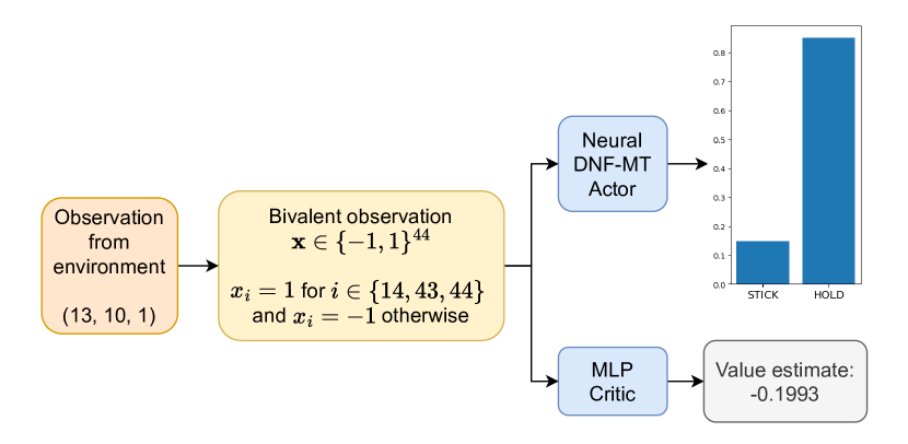
Figure 1. Neural DNF-MT model as an actor in actor-critic PPO, in environments with discrete observations.

Neural DNF-MT model in PPO algorithm for environments with categorical/factual observation.

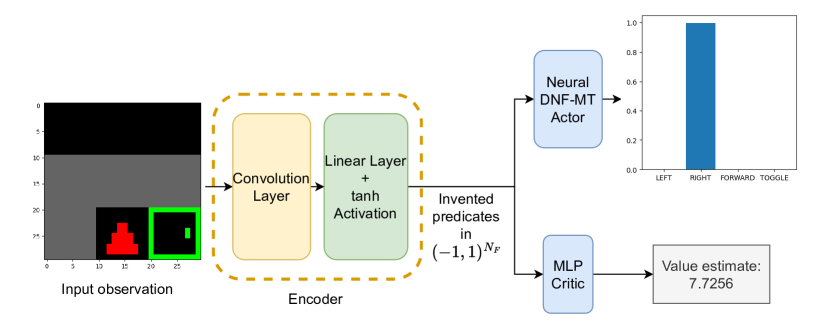
Figure 2. Neural DNF-MT model as an actor in actor-critic PPO, in environments with complex observations, such as an image-like multi-dimensional matrix.

Neural DNF-MT model in PPO algorithm for environments with complex observation.

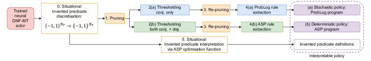
Figure 3. Post-training processing to extract an interpretable logical policy from a trained neural DNF-MT actor. There are two branches: one with sub-label (a) for extracting a stochastic policy in ProbLog and the other with sub-label (b) for extracting a deterministic policy in ASP.

Post-training pipeline for a trained neural DNF-MT actor.

We here present the overall training loss of the actor-critic PPO with a neural DNF-MT actor, which consists of multiple loss terms. The base training loss component matches that from PPO Schulman et al. (2017):

$$L^{\text{PPO}}(\theta)=\mathbb{E}_{t}\left[L^{\text{CLIP}}(\theta)+c_{1}L^{\text{value}}(\theta)-c_{2}S[\pi_{\theta}](s_{t})\right]$$ (4)

where $c_{1},c_{2}\in\mathbb{R}$ are hyperparameters, $L^{\text{CLIP}}(\theta)$ is the clipped surrogate objective, $S[\pi_{\theta}](s_{t})$ is the entropy of the actor in training, and $L^{\text{value}}(\theta)$ is the value loss. The detailed explanations for each term are in Appendix B.1. The action probability output of the neural DNF-MT actor defined in Eq (3) is used to calculate the probability ratio in $L^{\text{CLIP}}$ and the entropy term $S[\pi_{\theta}](s_{t})$.

We add the following auxiliary losses to facilitate the interpretation of the neural DNF-MT model into rules:

$$L^{(1)}(\theta) =\frac{1}{N_{F}}\sum_{i}^{N_{F}}\left|1-\left|f_{i}\right|\right|$$ (5)

$$L^{(2)}(\theta) =\frac{1}{|\theta_{\text{disj}}|}\sum|\theta_{\text{disj}}\cdot(6-|\theta_{\text{disj}}|)$$ (6)

$$L^{(3)}(\theta) =\frac{1}{N_{C}}\sum_{i}^{N_{C}}\left|1-\left|c_{i}\right|\right|$$ (7)

$$L^{(4)}(\theta) =-\sum_{i}^{N}\left[p_{i}\log\left(\frac{\hat{y}_{i}+1}{2}\right)+(1-p_{i})\log\left(1-\frac{\hat{y}_{i}+1}{2}\right)\right]$$ (8)

where $f_{i}$ is the invented predicate, $N_{F}$ is the number of output of an encoder, and $N_{C}$ is the number of conjunctive nodes. Eq (5) is used when there is an encoder before the neural DNF-MT actor for predicate invention. It enforces the predicates’ activations to be close to $\pm 1$ so that they are stronger beliefs of true/false. Eq (6) is a weight regulariser to encourage the disjunctive weights to be close to $\pm 6$ (the choice of $\pm 6$ is to saturate $\tanh$, as $\tanh(\pm 6)\approx\pm 1$). Eq (7) encourages the $\tanh$ output of the conjunctive layer to be close to $\pm 1$. Eq (8) is the key term to satisfy P2, pushing for bivalent logical interpretations for deterministic policies. This term mimics a cross-entropy loss between each mutex-tanh output and corresponding individual $\tanh$ outputs of the disjunctive layer, pushing the probability interpretations of the $\tanh$ outputs (i.e. $(\hat{y}_{i}+1)/2$) towards their action probability $\tilde{p}_{i}$ counterparts. If the optimal policy is deterministic, all $\tilde{p_{i}}$ will be approximately 0 except for one, which is close to 1. Each $\hat{y_{i}}$ is pushed towards $\pm 1$, and only one will be close to 1, thus having exactly one bivalent interpretation $b_{i}=\top$ and satisfying logical mutual exclusivity.

Finally, the overall training loss is defined as:

$$L(\theta)=L^{\text{PPO}}(\theta)+\sum_{i\in\{1,2,3,4\}}\lambda_{i}L^{(i)}(\theta)$$ (9)

where $\lambda_{i}\in\mathbb{R},i\in\{1,2,3,4\}$ are hyperparameters.

Post-training Processing.   This extracts either a ProbLog program for a stochastic policy or an ASP program for a close-to-deterministic policy from a trained neural DNF-MT actor, where the logic program is a close approximation of the model. It consists of multiple stages, as shown in Figure 3, described as follows.

(1) Pruning: This step repeatedly passes over each edge that connects an input to a conjunction or a conjunction to a disjunction, and removes any edge that can be removed (i) without changing the learned trajectory (for deterministic domains) or (ii) without shifting any action probability for any state more than some threshold $\tau_{\text{prune}}$ from the original learned policy (for stochastic domains). Any unconnected nodes are also removed. The process terminates when a pass fails to remove any edges or nodes.

(2) Thresholding: This process converts a semi-symbolic layer’s weights from $\mathbb{R}$ to values in $\{-6,0,6\}$. Given some threshold $\tau\in\mathbb{R}_{\geq 0}$, a new weight is computed as $w^{\prime}_{\text{k}ij}=6\cdot\mathbbm{1}_{|w_{\text{k}ij}|\geq\tau}(w_{\text{k}ij})\cdot\text{sign}(w_{\text{k}ij}),\text{k}\in\{\text{c},\text{d}\}$. This weight update enables the neural to bivalent logic translation described later. The selection of $\tau$ should maintain the model’s trajectory/action probability, subject to the same checks used in pruning. For a thresholded node with at least one non-zero weight, we replace its $\tanh$ activation with step function $h(x)=2\cdot\mathbbm{1}_{x>0}(x)-1$, changing its output’s range to $\{-1,1\}$. The thresholding process is applied differently to the disjunctive layer depending on the nature of the policy desired.

1. For stochastic policies: Only the conjunctive layer is thresholded, i.e. choosing a value of $\tau$, updating only its weights and changing the activation function. The disjunctive layer still outputs action probabilities.

2. For deterministic policies: Thresholding is applied to both the conjunctive and disjunctive layers: a single value $\tau$ is chosen and applied in both layers’ weight update, and both layers have their $\tanh$ activation replaced with the step function. This process is only possible if the model satisfies P2.

(3) Re-pruning: The pruning process from Step 1 is repeated.

(4) Logical rules extraction: All nodes (conjunctive and disjunctive) are converted into some form of logical rules. The thresholding process guarantees that all conjunctive nodes can be translated into bivalent logic representations. For a conjunctive node $c_{j}$, we consider the set $\mathcal{X}_{j}=\{i\in\{1..I\}|w^{\prime}_{\text{c}ij}\neq 0\}$, and $|\mathcal{X}_{j}|\neq 0$. We partition $\mathcal{X}_{j}$ into subsets $\mathcal{X}_{j}^{+}=\{i\in\mathcal{X}_{j}|w^{\prime}_{\text{c}ij}=6\}$ and $\mathcal{X}_{j}^{-}=\{i\in\mathcal{X}_{j}|w^{\prime}_{\text{c}ij}=-6\}$, and translate $c_{j}$ to an ASP rule of the form $conj_{j}\leftarrow\bigwedge_{i\in\mathcal{X}_{j}^{+}}atom_{i},\bigwedge_{i\in\mathcal{X}_{j}^{-}}(\text{not}\ atom_{i})$, where $atom_{i}$ is an atom for input $x_{i}$. The disjunctive nodes are interpreted differently depending on the desired policy type.

1. Stochastic policy - ProbLog rules: We use ProbLog’s annotated disjunctions to represent mutually exclusive action probabilities. Each unique achievable activation of the conjunctive layer $\mathbf{c}^{(m)}\in\{-1,1\}^{C^{\prime}}$ with $1\leq m\leq 2^{C^{\prime}}$ forms the body of a unique annotated disjunction of the form $p_{1}::action_{1};...;$ $p_{N}::action_{N}\leftarrow\bigwedge_{i\in\mathcal{C}^{(m)+}}conj_{i},\bigwedge_{i\in\mathcal{C}^{(m)-}}(\backslash+conj_{i})$, where $\mathcal{C}^{(m)+}=\{i|c^{(m)}_{i}=1\}$, $\mathcal{C}^{(m)-}=\{i|c^{(m)}_{i}=-1\}$, and $p_{j}=(\tilde{y}^{(m)}_{j}+1)/2$ (the probability assigned to the $j$^th action in the disjunctive activation for the $m^{\text{th}}$ unique activation). We compute such annotated disjunctions for all unique conjunctive activations. Listing 2 shows an example of ProbLog rules.

2. Deterministic policy - ASP rules: Since the disjunctive layer is also thresholded, we translate each disjunctive node into a normal clause. For a disjunctive node $d_{j}$, we consider the set $\mathcal{C}_{j}=\{i\in\{1..C^{\prime}\}|w^{\prime}_{\text{d}ij}\neq 0\}$, and $|\mathcal{C}_{j}|\neq 0$. We partition $\mathcal{C}_{j}$ into subsets $\mathcal{C}_{j}^{+}=\{i\in\mathcal{C}_{j}|w^{\prime}_{\text{d}ij}=6\}$ and $\mathcal{C}_{j}^{-}=\{i\in\mathcal{C}_{j}|w^{\prime}_{\text{d}ij}=-6\}$, and translate $d_{j}$ to a formula of the form $disj_{j}\leftarrow(\bigvee_{i\in\mathcal{C}_{j}^{+}}conj_{i})\vee(\bigvee_{i\in\mathcal{C}_{j}^{-}}(\text{not}\ conj_{i}))$. In practice, the formula is represented as multiple rules with the same head in ASP. Listing 1 shows an example of ASP rules.

If there is an encoder before the neural DNF-MT actor in the overall architecture, we perform a mandatory step of invented predicate discretisation (step 0 in Figure 3) at the beginning of the post-training process. We take the sign of the invented predicate $\tanh$ activations, converting them to $\pm 1$ to interpret them as bivalent logical truth values of $\top$ or $\bot$. Each invented predicate is defined as a minimal set of raw observations using an ASP optimisation function (step 5 in Figure 3).

Neural-bivalent-logic translation.  The translation for deterministic policies is bidirectional and maintains truth value equivalence: given an input tensor and its translated logical assignment, the interpreted bivalent truth value of the neural DNF-MT model with only $\pm 6$-and-0-valued weights is the same as the logical valuation of its translated ASP program, and vice versa. The proof that the translation is bidirectionally truth value equivalent is provided in Appendix A.

4. Experiments

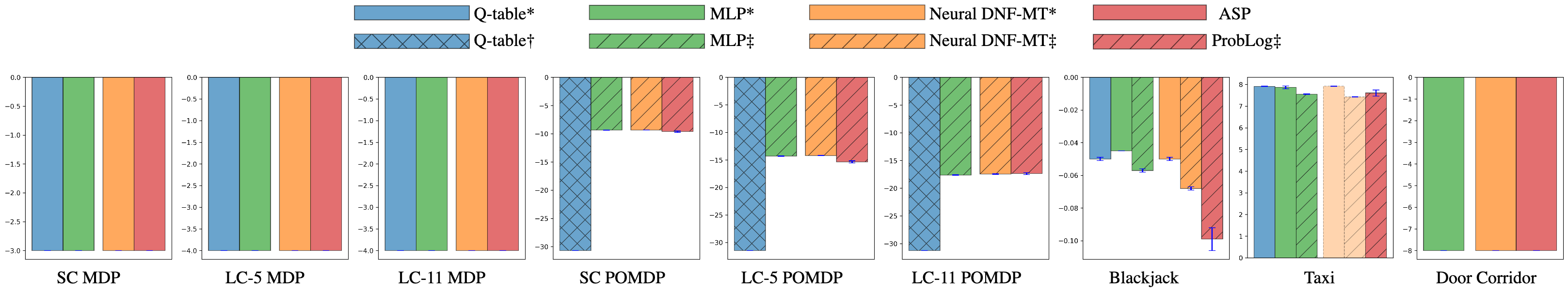
Figure 4. Mean episodic return $\pm$ standard error of the baselines and neural DNF-MT models, together with the ProbLog/ASP programs extracted from their corresponding neural DNF-MT models. All Q-tables are trained using Q-learning, and all MLP actors are trained with actor-critic PPO. Most neural DNF-MT actors are trained with actor-critic PPO. Except in the Taxi environment, the neural DNF-MT actor is distilled from a trained MLP actor (shown in dashed border and faded colour). Different symbols after the actor’s name indicate different action selection methods: * for argmax action selection, $\dagger$ for $\epsilon$-greedy sampling, and $\ddagger$ for actor’s distribution sampling. The same result is also reported in Table 5 in Appendix.

Performance of the models in all environments, together with the ProbLog/ASP programs extracted from their corresponding neural DNF-MT models.

We evaluate the RL performance (measured in episodic return) of our neural DNF-MT actors and their interpreted logical policies in four sets of environments with various forms of observations. Some tasks require stochastic behaviours, while others can be solved with deterministic policies. We compare our method with two baselines: Q-tables trained with Q-learning where applicable and MLP actors trained with actor-critic PPO. Our neural DNF-MT actors are trained with MLP critics using the PPO algorithm in the Switcheroo Corridor set, Blackjack and Door Corridor environments. In the Taxi environment, we distil a neural DNF-MT actor from a trained MLP actor. We do not directly evaluate the extracted ProbLog policies because of the long ProbLog query time. Instead, we evaluate their final neural DNF-MT actors before logical rule extraction (i.e. after step 3, re-pruning) as an approximation. The approximation is acceptable because a ProbLog policy’s action distribution is the same as its corresponding neural DNF-MT’s action distribution to 3 decimal places. A performance evaluation summary is shown in Figure 4, and a detailed version is presented in Table 5 in Appendix.

4.1. Switcheroo Corridor

We adopt an example environment from Sutton and Barto (2018) and create a set of Switcheroo Corridor environments that support MDP tasks with deterministic policies and POMDP tasks with stochastic policies. The observation can be either (i) the state number one-hot encoding of the agent’s current position (an MDP task) or the wall status of the agent’s current position (a POMDP task). In most states, going left or right results in moving in the intended direction. However, there are special states that reverse the action effect. Thus, the nature of the task decides whether the optimal policy is deterministic or stochastic. In the MDP setting, the optimal policy is deterministic: identifying the special states based on the state number and going left in them. In the POMDP setting, identifying the special states based solely on wall status observations is impossible without a memory. The optimal policy shows stochastic behaviour so that the correct action may be sampled in the special states.

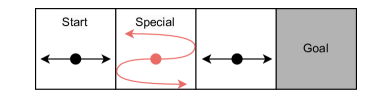
Figure 5. Small corridor (SC), same as the one from Sutton and Barto (2018).

Small Corridor environment - a visualisation of the environment. The agent starts at state 0 and needs to reach state 3 (0-indexed), and state 2 is the special state that reverses the action effect.

The start, goal, and special states are customisable but fixed once created throughout training and inference. We create three corridors based on different configurations: Small Corridor (SC) as shown in Figure 5, Long Corridor-5 (LC-5), and Long Corridor-11 (LC-11), to test the actor’s learning ability when the environment complexity increases. The configurations and the figures of LC-5 and LC-11 are listed in Appendix C.1.

The first six groups in Figure 4 show the performance of all models in the environment set. In MDP settings, all methods using argmax action selection perform equally well, reaching the goal with the minimum number of steps. In POMDP settings, MLP and neural DNF-MT actors perform better than Q-table with $\epsilon$-greedy sampling as expected, with minor performance differences. Neural DNF-MT actors provide interpretability via logical programs compared to MLP actors. Listing 1 shows the ASP program for a neural DNF-MT actor in SC MDP, where state 1 is identified as special. Listing 2 shows the ProbLog rules for a neural DNF-MT actor in SC POMDP. As shown in line 1 in Listing 2, the actor favours the action going right when only the left wall is present, which only happens in state 0. Line 2 shows the case when the agent is in either state 1 or 2 with no wall on either side, and the actor shows close to 50-50 preference for both actions. The logical representations for policies learned in LC-5 and LC-11 are included in Appendix D.1.

⬇

1action(left) :- in_s_1. action(right) :- not in_s_1.

Listing 1: ASP rules of a neural DNF-MT actor in SC MDP.

⬇

10.041::action(left) ; 0.959::action(right) :- left_wall_present, \+ right_wall_present.

20.581::action(left) ; 0.419::action(right) :- \+ left_wall_present, \+ right_wall_present.

Listing 2: ProbLog rules of a neural DNF-MT actor in SC POMDP.

4.2. Blackjack

The Blackjack environment from Sutton and Barto (2018) is a simplified version of the card game Blackjack, where the goal is to beat the dealer by having a hand closer to 21 without going over. The agent sees the sum of its hand, the dealer’s face-up card, and whether it has a usable ace. It can choose to hit or stick. The performance across the models is shown in the 7^th group in Figure 4 and Table 1. The baseline Q-table from Sutton and Barto (2018) only shows a single action, so we only evaluate it with argmax action selection. We evaluate the MLP and neural DNF-MT actors with both argmax action selection and actor’s distribution sampling. MLP actors with argmax action selection perform better than their distribution sampling counterparts, with a higher episodic return and win rate. The same is observed for neural DNF-MT actors. The extracted ProbLog rules perform worse than their original neural DNF-MT actors (no post-training processing). We observe a policy change (shown in Figures 10 and 11 in Appendix) that results in a higher policy divergence from the Q-table from Sutton and Barto (2018). This issue of performance loss occurs at the thresholding stage during the post-training processing and persists in later environments; we will discuss it further in Section 5.

Table 1. Blackjack: performance of MLP actors, neural DNF-MT actors, and the extracted ProbLog programs. Policy divergence measures the proportion of states where the argmax policy disagrees with the Q-table from Sutton and Barto (2018).

Model	Episodic return	Win rate	Policy Divergence
Q-table Sutton and Barto (2018)*	-0.050 $\pm$ 0.001	42.94% $\pm$ 0.00%	NA
MLP*	-0.045 $\pm$ 0.000	43.24% $\pm$ 0.02%	15.87% $\pm$ 0.30%
MLP$\ddagger$	-0.057 $\pm$ 0.001	42.84% $\pm$ 0.02%
NDNF-MT*	-0.050 $\pm$ 0.001	42.82% $\pm$ 0.06%	20.66% $\pm$ 0.56%
NDNF-MT$\ddagger$	-0.068 $\pm$ 0.001	42.17% $\pm$ 0.03%
ProbLog$\ddagger$	-0.099 $\pm$ 0.007	40.79% $\pm$ 0.31%	27.92% $\pm$ 1.25%

4.3. Taxi

In the Taxi environment (Figure 9 in Appendix) from Dietterich (2000), the agent controls a taxi to pick up a passenger first and drop them off at the destination hotel. A state number is used as the observation, and it encodes the taxi, passenger and hotel locations using the formula $((taxi\_row*5+taxi\_col)*5+passenger\_loc)*4+destination$. Apart from moving in four directions, the agent can pick up/drop off the passenger, but illegally picking up/dropping off will be penalised. The environment is designed for hierarchical reinforcement learning but is solvable with PPO and without task decomposition. However, we find that model performance is more sensitive to PPO’s hyperparameters and fine-tuning the hyperparameters is more difficult than in other environments. With the wrong set of hyperparameters, the actor settles at a local optimal with a reward of -200: never perform ‘pickup’/‘drop-off’ and move until the step limit (200 steps). The environment is complex due to its hierarchical nature, and learning the task dependencies based on purely state numbers proves to be difficult, as a 1-value change in the x/y coordinate of the taxi results is a change of state number in 100s/10s. We successfully trained MLP actors with actor-critic PPO but failed to find a working set of hyperparameters to train neural DNF-MT actors. Instead, we distil a neural DNF-MT actor from a trained MLP actor, taking the same observation as input and aiming to output the exact action probabilities as the MLP oracle.

The performance is shown in the 8^th group in Figure 4. Actors using argmax action selection perform better than their distribution sampling counterparts. Again, we observe a performance drop in extracted ProbLog rules. With 300 unique possible starting states, the extracted ProbLog rules are not guaranteed to finish in 200 steps: 2 out of the 10 ProbLog evaluations with action probabilities sampling have truncated episodes. Across ten post-training-processed neural DNF-MT actors with argmax action selection, there are an average of 3.3 unique starting states where the models cannot finish the environment within 200 steps. De-coupling the observation seems complicated and makes it hard to learn concise conjunctions, thus increasing the error rate in the post-training processing.

4.4. Door Corridor

Inspired by Minigrid Chevalier-Boisvert et al. (2023), we design a corridor grid with a fixed configuration called Door Corridor, as shown in Figure 6. The agent observes a $3\times 3$ grid in front of it (as shown as the input in Figure 2) and has a choice of four actions: turn left, turn right, move forward, and toggle. The toggle action only changes the status of a door right in front of the agent.

For this environment, we use the architecture shown in Figure 2, where an encoder is shared between the actor and the critic. The performance of MLP actors, neural DNF-MT actors and their extracted ASP programs is shown in the last group in Figure 4. Both of the neural actors learn the optimal deterministic policy.

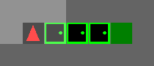
Figure 6. Door Corridor (DC): the agent needs to turn right first, and toggle and go through 3 doors to reach the end of the corridor.

Door Corridor environment - an image visualising the environment.

To evaluate an extracted ASP program in the environment, we first pass the $3\times 3$ observation to the encoder, convert invented predicates with bivalent interpretations $\top$ to ASP facts, and then append these facts as context to the base policy. The combined ASP program has to (i) output one stable model with only one action at each step (logically mutual exclusive) and (ii) finish without truncation to be counted as a successful run. These requirements are also reflected in the neural DNF-MT actor: the final $\tanh$ activation should only have one value greater than 0, and taking that only action with greater-than-0 $\tanh$ activation at each step finishes the environment without truncation. During post-training processing, 3 out of 16 neural DNF-MT runs have issues at the thresholding stage: either more than one $\tanh$ activation is greater than 0, or none is greater than 0. Although it is possible to extract ProbLog programs from these three runs, we desire deterministic policies from the trained neural DNF-MT actors instead of stochastic ones. Hence, no logical programs are extracted from them. The ASP programs of the remaining 13 runs successfully finish the environment with minimal steps, as reported in Figure 4. Listing 3 shows an example of the extracted ASP program from one of the successful runs, together with a possible set of definitions for the invented predicates.

⬇

1action(turn_right) :- not a_9, a_13, not a_14.

2action(forward) :- not a_8.

3action(toggle) :- a_9.

4

5% Definitions of each invented predicate a_i:

6a_8 :- top_right_corner_unseen.

7a_9 :- one_step_ahead_closed_door.

8a_13 :- not one_step_ahead_open_door.

9a_14 :- curr_location_open_door.

Listing 3: An ASP policy for a neural DNF-MT actor in DC, with a possible set of defintions for the invented predicates.

Policy Intervention.   We create two variations of the base Door Corridor environment with different termination conditions: Door Corridor-T (DC-T), where the agent must be in front of the goal and toggle it instead of moving into it, and Door Corridor-OT (DC-OT), where the agent must stand on the goal and take the action ‘toggle’. The input observation remains unchanged since only the goal cell’s mechanism changes. The encoder can be reused immediately, but the actor and critic cannot. An MLP actor trained on DC fails to finish within step limits in DC-T and DC-OT environments without re-training. However, we can modify the ASP policy to achieve the optimal reward in both DC-T and DC-OT environments. Listings 4 and 5 show the modified ASP programs for DC-T and DC-OT environments, respectively. The modified ASP programs can be ported back to neural DNF-MT actors by virtue of the bidirectional neural-bivalent-logic translation. The modified neural DNF-MT actors also finish DC-T and DC-OT environments with minimal steps without any re-training.

⬇

1action(turn_right) :- not a_9, a_13, not a_14.

2action(forward) :- not a_8, not a_13.

3action(toggle) :- a_9.

4$\textbf{action(toggle) :- a\_11, a\_13}.$

Listing 4: Policy for DC-T, modified from Listing 3’s policy.

⬇

1action(turn_right) :- not a_9, not a_10, a_13, not a_14.

2action(forward) :- not a_8.

3action(toggle) :- a_9.

4$\textbf{action(toggle) :- a\_8, not a\_9, a\_10}.$

Listing 5: Policy for DC-OT, modified from Listing 3’s policy.

5. Discussions

We first analyse the persistent performance loss issue in Blackjack, Taxi, and Door Corridor environments.

Performance loss due to thresholding.  The thresholding step converts the target layer(s) from a weighted continuous space to a discrete space with only 0 and $\pm 6$ values, saturating the $\tanh$ activation at $\pm 1$ and enabling the translation to bivalent logic. However, the thresholding step may not maintain the same logical interpretation of the layer output, as shown in Listing 6, where a thresholded neural DNF-MT actor fails to maintain logical mutual exclusivity in the Door Corridor environment. Note that we apply thresholding on both the conjunctive and disjunctive layers since we desire a deterministic policy from the model. The 1^st row of values in Table 2 are the pre-thresholding $\tanh$ output when $x_{2}=-1,x_{7}=1,x_{9}=1,x_{13}=-1$ , with $\hat{y_{3}}$ interpreted as $\top$ and chosen as action. The thresholded conjunctive nodes in the 2^nd row share the same sign as row 1, but $\hat{y_{3}}$ becomes positive after thresholding, resulting in two actions being $\top$ and thus violating logical mutual exclusivity. The original weights of the disjunctive nodes achieve the balance of importance between $c_{7}$, $c_{9}$ and $c_{11}$ to make $\hat{y_{3}}$ negative. However, the thresholding process ignores the weights and makes them equally important, leading to a different output and truth value. It shows that the thresholding stage cannot handle volatile and interdependent weights and maintain the underlying truth table represented by the model. We leave it as a future work to improve/replace the thresholding stage with a more robust method.

⬇

1% Conjunctive nodes:

2c_0 = 3.03 x_7 + bias_c0

3c_7 = 0.56 x_13 + bias_c7

4c_9 = -1.56 x_2 + bias_c9

5c_11 = -1.05 x_9 + bias_c11

6

7% Disjunctive nodes:

8d_1 = 4.58 c_0 + bias_d1

9d_2 = -3.48 c_9 + bias_d2

10d_3 = 1.29 c_7 + 0.76 c_9 + 4.33 c_11 + bias_d3

11

12% Thresholded nodes with tau = 0 (and ASP translation):

13c_0 = 6 x_7 (conj_0 :- a_7.)

14c_7 = 6 x_13 (conj_7 :- a_13.)

15c_9 = -6 x_2 (conj_9 :- not a_2.)

16c_11 = -6 x_9 (conj_11 :- not a_9.)

17d_1 = 6 c_0 (act(1) :- conj_0.)

18d_2 = -6 c_9 (act(2) :- not conj_9.)

19d_3 = 6 c_7 + 6 c_9 + 6 c_11 + 12

20(act(3) :- conj_7. act(3) :- conj_9. act(3) :- conj_11.)

Listing 6: A neural DNF-MT actor in the Door Corridor environment that fails at the thresholding stage. We leave the bias terms uncalculated for brevity.

Table 2. Conjunctive and disjunctive nodes’ $\tanh$ output when $x_{2}=-1,x_{7}=1,x_{9}=1,x_{13}=-1$, calculated based on the formulation in Listing 6. Row 1 is the original output without applying thresholding, and row 2 is the output after thresholding on value 0.

$c_{0}$	$c_{7}$	$c_{9}$	$c_{11}$	$\hat{y_{1}}$	$\hat{y_{2}}$	$\hat{y_{3}}$
1.00	-0.51	0.92	-0.78	1.00	-1.00	-0.86
1.00	-1.00	1.00	-1.00	1.00	-1.00	1.00

We now discuss the implications of our work in terms of performance, interpretability, inference, and policy intervention.

Performance.   From the experiments, we see that the neural DNF-MT actor can be trained with actor-critic PPO or distilled from an MLP oracle to learn an optimal policy in the Switcheroo Corridor, Taxi, and Door Corridor environments. In Blackjack, the performance is worse but close to an optimal MLP actor. Furthermore, we demonstrate that an encoder for handling complex observations and realising predicate invention can be end-to-end trained with the neural DNF-MT actor in the Door Corridor environment.

Interpretability.   The logical programs extracted from trained neural DNF-MT actors provide interpretability, which MLP actors lack. We also demonstrate through different environments that we can represent stochastic and deterministic policies in different forms of logic (ProbLog and ASP, respectively).

Inference.   While knowing what the actor has learnt is useful, running a fully logic-based agent might not be sensible. We find that inference in neural DNF-MT actors is significantly faster than in ProbLog or ASP, thanks to tensor operations and environment parallelism (see Appendix E for detailed comparison).

Policy Intervention.   The bidirectional neural-bivalent-logic translation allows us to modify the ASP program and translate it back to the neural architecture without re-training, as shown in Door Corridor’s variations in Section 3. This feature could be helpful in tasks where we have background knowledge. By pre-encoding the information into logical rules or modifying the logical rules of an actor trained in a similar environment, the edited logic program can be ported back to the neural model to provide a hot start in training. This functionality will be explored in future work.

In summary, our neural DNF-MT model learns interpretable and editable policies, with the neural benefits of end-to-end training and parallelism in inference and the logical benefits of interpretable logical program representation.

6. Related Work

Many neuro-symbolic approaches perform the task of inductive logic programming (ILP) Muggleton and de Raedt (1994); Cropper et al. (2022) in differentiable models, and policies are learned and represented as logical rules. They are commonly applied in Relational RL Džeroski et al. (2001); Zambaldi et al. (2018) domains that utilise symbolic representations for states, actions, and policies. NLRL Jiang and Luo (2019) and NUDGE Delfosse et al. (2023) are two approaches based on the differentiable ILP system Evans and Grefenstette (2018) and its extension from Shindo et al. (2021), where the search space needs to be defined first. NLRL generates candidate rules using rule templates. NUDGE distils symbolic policy from a trained neural model by defining its search space with mode declarations Muggleton (1995) and then training rule-associated weights. NeSyRL Kimura et al. (2021) and Differentiable Logic Machine (DLM) Zimmer et al. (2021) do not associate weights with rules but predicates; thus, they are not reliant on rule templates or mode declarations. NeSyRL uses a disjunctive normal form Logical Neural Network (LNN) Riegel et al. (2020) as its actor, and each neuron represents an atom/logical connective. A pre-trained semantic parser extracts first-order logic predicates from text-based observations, and the LNN selects actions to generate trajectories that get stored in a replay buffer for training, similar to DQN Mnih et al. (2015). DLM builds upon Neural Logic Machine Dong et al. (2019) to realise forward chaining, but with logical computation units to provide interpretability. A DLM actor is trained with actor-critic PPO Schulman et al. (2017), with a specially designed critic with GRUs to handle different-arity predicates.

Different from NLRL Jiang and Luo (2019) and NUDGE Delfosse et al. (2023), our neural DNF-MT model does not use rule templates or mode declarations. Therefore, it does not rely on human engineering to construct the inductive bias and can learn a wider range of rules. Compared to the mentioned works that either operate on relational-based observations Jiang and Luo (2019); Delfosse et al. (2023); Zimmer et al. (2021) or require pre-trained networks to extract logical predicates Delfosse et al. (2023); Kimura et al. (2021), we demonstrate that our neural DNF-MT model is end-to-end trainable with preceding layers for predicate invention. Akin to DLM Zimmer et al. (2021), we use the PPO algorithm for training; however, our method does not require a specialised critic.

7. Conclusion

We propose a neuro-symbolic approach named the neural DNF-MT model for learning interpretable and editable policy in RL. It can be trained with actor-critic PPO or distilled from a trained MLP actor, and an encoder for predicate invention can also be end-to-end trained together with it. The trained neural DNF-MT model can be represented as either a ProbLog program for stochastic policy or an ASP program for deterministic policy. The neural-bivalent-logic translation is bidirectional, allowing policy intervention by modifying the ASP program and then converting it back to the neural model for efficient inference in parallel environments. We evaluate the neural DNF-MT model in four environments with different forms of observations and stochastic/deterministic behaviours. The experiments show the neural DNF-MT model’s capability to learn the optimal policy with performance similar to an MLP actor’s. Furthermore, it provides logical representation and use cases for policy intervention, neither of which can be provided easily by an MLP. In future work, we aim to follow up on the policy intervention idea by providing the neural DNF-MT actor with a hot starting point from a modified policy. Moreover, the thresholding stage during post-training processing needs to be improved/replaced so that the underlying logical relations learned by the neural DNF-MT model can be extracted without performance loss.

Appendix A Neural-bivalent-logic Translation

This section focuses on proving that the neural-bivalent-logic translation bidirectionally maintains the logical truth value equivalence. We first mention some important properties of semi-symbolic nodes, then prove that the translation from neural to bivalent logic has the same inference truth value and vice versa. The proof is done for a conjunctive node, and a disjunctive node’s proof is similar.

A.1. Semi-symbolic Node Properties

Consider a node in a semi-symbolic layer with $I$ inputs, and its weights $\mathbf{w}\in\{-6,0,6\}^{I}$ and at least one is non-zero (i.e. $\exists i\in\{1..I\}.w_{i}\neq 0$), it has either of the following two properties:

Remark 0.

If the node is conjunctive, with $I$ inputs and at least one non-zero weight: given an input tensor $\mathbf{x}$ to it, and $\forall i\in\{1..I\}.w_{i}\in\{-6,0,6\},x_{i}\in\{-1,1\}$, the node’s raw output will never be 0. It can be 6 or less than or equal to -6. Since $\tanh(\pm 6)=\pm 0.99998771165$, the conjunctive node’s $\tanh$ activation is treated to be exactly $\pm 1$ for the forward evaluation; or we can replace the $\tanh$ activation with a step function that maps the range to $\{-1,1\}$, as mentioned in the thresholding process in Section 3.3.

Remark 0.

If the node is disjunctive, with $I$ inputs and at least one non-zero weight: given an input tensor $\mathbf{x}$ to it, and $\forall i\in\{1..I\}.w_{i}\in\{-6,0,6\},x_{i}\in\{-1,1\}$, the node’s raw output will never be 0. It can be -6 or greater or equal to 6. Like the conjunctive node, the disjunctive node’s activation is $\pm 1$.

We focus on solving the combined program of the rule translated from a semi-symbolic node with weights $\mathbf{w}\in\{-6,0,6\}^{I}$, and the facts translated from an input $\mathbf{x}\in\{-1,1\}^{I}$. If an input/conjunction is connected to a conjunctive/disjunctive node with a weight of value $-6$, it can be translated to a literal with either classical negation (‘-’) or negation as failure (NAF, ‘not’) and then added as part of the rule body. Similarly, any $x_{i}=-1$ can be either mapped to a fact with classical negation ‘-a_i’, or not added to the program and ‘not a_i’ would be true. The inference result of the rules is the same regardless of whether the classical negation or NAF translation is chosen. We choose the NAF style of translation across the paper and proof.

A.2. Neural to Bivalent Logic Translation with Truth Value Equivalence

We have a conjunctive node with $I$ inputs in a semi-symbolic layer, and its weights are $\mathbf{w}$ and $\delta=1$. Let an input to the node be $\mathbf{x}$ and $g(\mathbf{x})$ be the raw output of the conjunctive node without any activation. The following conditions also hold for this node:

$$\mathbf{w}\in\{-6,0,6\}^{I}, \exists i\in\{1..I\}.w_{i}\neq 0$$ (10)

$$\mathbf{x} \in\{-1,1\}^{I}$$ (11)

Recall the bivalent logic translation we defined in Definition 3.1. Let $b$ be the bivalent logical interpretation of this conjunctive node. And $b=\top$ if $\tanh(g(\mathbf{x}))>0$, and $b=\bot$ otherwise.

We specifically consider the set $\mathcal{X}=\{i|i\in\{1..I\},w_{i}\neq 0\}$, and $|\mathcal{X}|\neq 0$. By construction, $\forall i\in\mathcal{X}.|w_{i}|=6$. We further divide set $\mathcal{X}$ into two mutually exclusive subsets:

$$\mathcal{X}^{+} =\left\{i|i\in\mathcal{X},w_{i}=6\right\}$$

$$\mathcal{X}^{-} =\left\{i|i\in\mathcal{X},w_{i}=-6\right\}$$

By construction, $\mathcal{X}^{+}\cap\mathcal{X}^{-}=\emptyset$ and $|\mathcal{X}^{+}|+|\mathcal{X}^{-}|=|\mathcal{X}|$.

We translate the conjunctive node to an ASP rule, and the translated rule is in the form:

$$h\leftarrow\bigwedge_{i\in\mathcal{X}^{+}}a_{i},\bigwedge_{i\in\mathcal{X}^{-}}(\text{not}\ a_{i})$$ (12)

We translate an input $\mathbf{x}\in\{-1,1\}^{I}$ to facts, and the set of facts are:

$$\{a_{i}.|i\in\{1..I\},x_{i}=1\}$$ (13)

Proposition

Given a conjunctive semi-symbolic node that satisfies Conditions (10) and its translated ASP rule with rule head $h$ based on Translation (12), and an input tensor $\mathbf{x}$ that satisfies Condition (11) and its translated facts based on Translation (13), the bivalent logical interpretation $b$ of the conjunctive semi-symbolic node from the input tensor $\mathbf{x}$ is the same as the truth value of the rule head $h$ evaluated with the joint ASP program of the translated rule and facts.

Proof.

Under Condition(10), the bias of the conjunctive node is calculated as follows, using Eq (1):

$$\beta=\max_{i=1}^{I}|w_{i}|-\sum_{i=1}^{I}|w_{i}|=6-\sum_{i\in\mathcal{X}}6=6-6|\mathcal{X}|$$

So we calculate the output of the conjunctive node as follows:

$$g(\mathbf{x}) =\sum_{i=1}^{I}w_{i}x_{i}+\beta$$

$$=6\sum_{i\in\mathcal{X}^{+}}x_{i}-6\sum_{i\in\mathcal{X}^{-}}x_{i}+(6-6|\mathcal{X}|)$$

Based on the input values specified in Condition (11), we can further split $\mathcal{X}^{+}$ and $\mathcal{X}^{-}$ into four mutually exclusive subsets:

$$\mathcal{X}^{++} =\{i|i\in\mathcal{X}^{+},x_{i}=1\}$$

$$\mathcal{X}^{+-} =\{i|i\in\mathcal{X}^{+},x_{i}=-1\}$$

$$\mathcal{X}^{-\phantom{}-} =\{i|i\in\mathcal{X}^{-},x_{i}=-1\}$$

$$\mathcal{X}^{-+} =\{i|i\in\mathcal{X}^{-},x_{i}=1\}$$

By construction, we have $\mathcal{X}^{++}\cap\mathcal{X}^{+-}=\emptyset$, $\mathcal{X}^{-\phantom{}-}\cap\mathcal{X}^{-+}=\emptyset$, and the followings:

$$|\mathcal{X}^{++}|+|\mathcal{X}^{+-}| =|\mathcal{X}^{+}|$$

$$|\mathcal{X}^{-\phantom{}-}|+|\mathcal{X}^{-+}| =|\mathcal{X}^{-}|$$

$$|\mathcal{X}^{++}|+|\mathcal{X}^{+-}|+|\mathcal{X}^{-\phantom{}-}|+|\mathcal{X}^{-+}| =|\mathcal{X}|$$

Thus, we can calculate the output of the conjunctive node as:

$$g(\mathbf{x}) =6\sum_{i\in\mathcal{X}^{+}}x_{i}-6\sum_{i\in\mathcal{X}^{-}}x_{i}+(6-6|\mathcal{X}|)$$

$$=6\left(\sum_{i\in\mathcal{X}^{++}}1+\sum_{i\in\mathcal{X}^{+-}}(-1)-\sum_{i\in\mathcal{X}^{-\phantom{}-}}(-1)-\sum_{i\in\mathcal{X}^{-+}}1+1-|\mathcal{X}|\right)$$

$$=6(|\mathcal{X}^{++}|-|\mathcal{X}^{+-}|+|\mathcal{X}^{-\phantom{}-}|-|\mathcal{X}^{-+}|-|\mathcal{X}|+1)$$

$$=6(1-2|\mathcal{X}^{+-}|-2|\mathcal{X}^{-+}|)$$ (14)

Now, based on Remark A.1, we consider the two case of $g(\mathbf{x})$.

Case 1: $g(\mathbf{x})=6>0$. The conjunctive node’s bivalent logical interpretation $b=\top$. We need to prove that $h$ from Translation (12) is in the answer set (i.e. $h$ is true).

By $g(\mathbf{x})=6$ and Eq (14):

$$1-2|\mathcal{X}^{+-}|-2|\mathcal{X}^{-+}| =1$$

$$|\mathcal{X}^{+-}|+|\mathcal{X}^{-+}| =0$$

$$\Rightarrow\mathcal{X}^{++}=\mathcal{X}^{+},\mathcal{X}^{-\phantom{}-} =\mathcal{X}^{-}$$ (15)

Combine Eq (15) with Translation (13), the ASP facts are:

$$\{a_{i}.|i\in\mathcal{X}^{+}|\}$$ (16)

Since:

$$\forall i\in\mathcal{X}^{+}.a_{i}\text{ is true} \Rightarrow\bigwedge_{i\in\mathcal{X}^{+}}a_{i}\text{ is true}$$

$$\forall i\in\mathcal{X}^{-}.\text{not}\ a_{i}\text{ is true} \Rightarrow\bigwedge_{i\in\mathcal{X}^{-}}(\text{not}\ a_{i})\text{ is true}$$

The combined program of (16) and (12) has the answer set with $h$ in it (i.e. $h$ is true).

Case 2: $g(\mathbf{x})\leq-6<0$. The conjunctive node’s bivalent logical interpretation $b=\bot$. We need to prove that $h$ from Translation (12) is not in the answer set (i.e. $h$ is false).

By $g(\mathbf{x})\leq-6$ and Eq (14):

$$1-2|\mathcal{X}^{+-}|-2|\mathcal{X}^{-+}| \leq-1$$

$$|\mathcal{X}^{+-}|+|\mathcal{X}^{-+}| \geq 1$$ (17)

We can split Eq (17) into three cases:

(a): If $|\mathcal{X}^{+-}|=0,|\mathcal{X}^{-+}|\geq 1$.

By $|\mathcal{X}^{+-}|=0$, we have $\mathcal{X}^{++}=\mathcal{X}^{+}$. Combined with Translation (13), we have the ASP facts:

$$\{a_{i}.|i\in\mathcal{X}^{+}\cup i\in\mathcal{X}^{-+}\}$$ (18)

We have:

$$\forall i\in\mathcal{X}^{+}.a_{i}\text{ is true} \Rightarrow\bigwedge_{i\in\mathcal{X}^{+}}a_{i}\text{ is true}$$

$$\exists i\in\mathcal{X}^{-}.a_{i}\text{ is true} \Rightarrow\bigwedge_{i\in\mathcal{X}^{-}}(\text{not}\ a_{i})\text{ is false}$$

Thus, the combined program of (18) and (12) has the answer set with $h$ not in it (i.e. $h$ is false).

(b): If $|\mathcal{X}^{+-}|\geq 1,|\mathcal{X}^{-+}|=0$.

By $|\mathcal{X}^{+-}|\geq 1$, we have $\mathcal{X}^{+-}\neq\mathcal{X}^{+}$. And by $|\mathcal{X}^{-+}|=0$, we have $\mathcal{X}^{-\phantom{}-}=\mathcal{X}^{-}$. Combine with Translation (13), we have the ASP facts:

$$\{a_{i}.|i\in\mathcal{X}^{++}\}$$ (19)

We have:

$$\exists i\in\mathcal{X}^{+}.a_{i}\text{ is not true} \Rightarrow\bigwedge_{i\in\mathcal{X}^{+}}a_{i}\text{ is false}$$

Thus, the combined program of (19) and (12) has the answer set with $h$ not in it (i.e. $h$ is false).

(c): If $|\mathcal{X}^{+-}|\geq 1,|\mathcal{X}^{-+}|\geq 1$.

This case is a combination of the previous two cases, and we can similarly prove that $h$ is not in the answer set (i.e. $h$ is false).

We have proved that the bivalent logical interpretation $b$ of the conjunctive semi-symbolic node equals the translated rule head $h$’s truth value in both cases. ∎

A.3. Bivalent Logic to Neural Translation with Truth Value Equivalence

There are $I$ different possible facts $a_{1},a_{2},...a_{I}$. Consider an ASP rule with head $h$ in the form of:

$$h\leftarrow\bigwedge_{i\in\mathcal{X}^{+}}a_{i},\bigwedge_{i\in\mathcal{X}^{-}}(\text{not}\ a_{i})$$ (20)

where $\mathcal{X}^{+}$ and $\mathcal{X}^{-}$ are the sets of IDs of the positive and negative literals in the rule. The following conditions hold:

$$\mathcal{X}^{+}\subseteq I,\mathcal{X}^{-}\subseteq I, |\mathcal{X}^{+}|\geq 0,|\mathcal{X}^{-}|\geq 0$$ (21)

$$\mathcal{X}^{+}\cap\mathcal{X}^{-} =\emptyset$$ (22)

We define the set $\mathcal{X}=\mathcal{X}^{+}\cup\mathcal{X}^{-}$, and $|\mathcal{X}|\neq 0$.

This rule can be translated to a conjunctive semi-symbolic node with $I$ inputs and $\delta=1$, and the weights are:

$$\forall i\in\{1..I\}.\ \ w_{i}=\begin{cases}6&\text{if }i\in\mathcal{X}^{+}\\ -6&\text{if }i\in\mathcal{X}^{-}\\ 0&\text{otherwise}\end{cases}$$ (23)

Again, let $b$ be the bivalent logical interpretation of the conjunctive node as defined in Definition 3.1.

We translate an ASP program of a set of facts $\mathcal{P}=\{a_{i}.|i\in\{1..I\}\}$ to an input tensor $\mathbf{x}$ as:

$$\forall i\in\{1..I\}.\ \ x_{i}=\begin{cases}1&\text{if }a_{i}\in\mathcal{P}\\ -1&\text{otherwise}\end{cases}$$ (24)

Proposition

Given an ASP rule in the form of (20) with head $h$ that satisfies Conditions (21) and (22) and its translated conjunctive semi-symbolic node with weights based on Translation (23), and the set of facts ASP program and its translated input tensor based on Translation (24), the truth value of $h$ evaluated with the joint ASP program of the rule and facts is the same as the bivalent logical interpretation $b$ of the translated conjunctive semi-symbolic node computed from the translated input tensor.

Proof.

Let the translated conjunctive node’s output be $g(\mathbf{x})$ and the bias of the node be $\beta$. Under the Conditions of (21) and (22), the bias is calculated as:

$$\beta=\max_{i=1}^{I}|w_{i}|-\sum_{i=1}^{I}|w_{i}|=6-6|\mathcal{X}|$$

So the output of the conjunctive node is:

$$g(\mathbf{x}) =\sum_{i=1}^{I}w_{i}x_{i}+\beta$$

$$=6\sum_{i\in\mathcal{X}^{+}}x_{i}-6\sum_{i\in\mathcal{X}^{-}}x_{i}+(6-6|\mathcal{X}|)$$ (25)

We consider two cases:

Case 1: $h$ is in the answer set (i.e. $h$ is true).

From it, we know that:

$$\forall i\in\mathcal{X}^{+}. a_{i}\text{ is true}$$

$$\forall i\in\mathcal{X}^{-}. \text{not}\ a_{i}\text{ is true}$$

Combined with Translation (24), we have:

$$\forall i\in\mathcal{X}^{+}. x_{i}=1$$

$$\forall i\in\mathcal{X}^{-}. x_{i}=-1$$

Substitute the values into the conjunctive node’s output in Eq (A.3):

$$g(\mathbf{x}) =6\sum_{i\in\mathcal{X}^{+}}1-6\sum_{i\in\mathcal{X}^{-}}(-1)+(6-6|\mathcal{X}|)$$

$$=6(|\mathcal{X}^{+}|+|\mathcal{X}^{-}|+1-|\mathcal{X}|)$$

By Condition (22), we have $|\mathcal{X}^{+}|+|\mathcal{X}^{-}|=|\mathcal{X}|$. Thus:

$$g(\mathbf{x}) =6>0$$

$$b =\top=h$$

Case 2: $h$ is not in the answer set (i.e. $h$ is false).

We further split $\mathcal{X}^{+}$ and $\mathcal{X}^{-}$ into four mutually exclusive subsets:

$$\begin{split}\mathcal{X}^{++}&=\{i|i\in\mathcal{X}^{+},a_{i}\in\mathcal{P}\}\\ \mathcal{X}^{+-}&=\{i|i\in\mathcal{X}^{+},a_{i}\notin\mathcal{P}\}\\ \mathcal{X}^{-\phantom{}-}&=\{i|i\in\mathcal{X}^{-},a_{i}\notin\mathcal{P}\}\\ \mathcal{X}^{-+}&=\{i|i\in\mathcal{X}^{-},a_{i}\in\mathcal{P}\}\end{split}$$ (26)

For $h$ to be not in the answer set, the following must hold:

$$|\mathcal{X}^{+-}|+|\mathcal{X}^{-+}|\geq 1$$

such that either or both of $\bigwedge_{i\in\mathcal{X}^{+-}}a_{i}$ and $\bigwedge_{i\in\mathcal{X}^{-+}}(\text{not}\ a_{i})$ are false.

Combine the subsets in (26) with Translation (24) and the input tensor $\mathbf{x}$ should be like:

$$\forall i\in\mathcal{X}^{++}. x_{i}=1$$

$$\forall i\in\mathcal{X}^{+-}. x_{i}=-1$$

$$\forall i\in\mathcal{X}^{-\phantom{}-}. x_{i}=-1$$

$$\forall i\in\mathcal{X}^{-+}. x_{i}=1$$

Substitute the values into the output of the conjunctive node in Eq (A.3), we have:

$$g(\mathbf{x}) =6\left(\sum_{i\in\mathcal{X}^{++}}1+\sum_{i\in\mathcal{X}^{+-}}(-1)\right)-6\left(\sum_{i\in\mathcal{X}^{-\phantom{}-}}(-1)+\sum_{i\in\mathcal{X}^{-+}}1\right)+(6-6|\mathcal{X}|)$$

$$=6(|\mathcal{X}^{++}|-|\mathcal{X}^{+-}|+|\mathcal{X}^{-\phantom{}-}|-|\mathcal{X}^{-+}|-|\mathcal{X}|+1)$$

$$=6(1-2|\mathcal{X}^{+-}|-2|\mathcal{X}^{-+}|)$$

Since $|\mathcal{X}^{+-}|+|\mathcal{X}^{-+}|\geq 1$, we have $1-2|\mathcal{X}^{+-}|-2|\mathcal{X}^{-+}|\leq-1$. Hence:

$$g(\mathbf{x}) \leq-6$$

$$\Rightarrow b =\bot=h$$

We have proved that the rule head $h$’s truth value equals the bivalent logical interpretation $b$ of the translated conjunctive semi-symbolic node in both cases. ∎

Appendix B Training Details

We use PyTorch Ansel et al. (2024) for implementing the neural DNF-MT actors and MLP baselines, and CleanRL Huang et al. (2022) for the base implementation of actor-criticy PPO. We also adopt the training technique of $\delta$ scheduling for neural DNF-based models used in Cingillioglu and Russo (2021) and Baugh et al. (2023). At each training iteration $i$, the $\delta$ value is calculated as:

$$m ={\left\lfloor\frac{i-d}{s}\right\rfloor+1}$$

$$\delta_{\text{new}} =\delta_{\text{initial}}*r^{m}$$

where $d$ is the delay, $s$ is the ‘decay’ step size, $\delta_{\text{initial}}$ is the initial $\delta$ value and $r$ is the ‘decay’ rate, which all are hyperparameters.

The implementation of neural DNF-based models is at https://anonymous.4open.science/r/neural-dnf-BE3E/README.md and our training and evaluation code is at https://anonymous.4open.science/r/ndnf_rl-B08D/README.md.

B.1. Base PPO Loss

The PPO loss function based on the original PPO paper Schulman et al. (2017) and CleanRL Huang et al. (2022) is represented as:

$$L^{\text{PPO}}(\theta) =\mathbb{E}_{t}\left[L^{\text{CLIP}}(\theta)+c_{1}L^{\text{value}}(\theta)-c_{2}S[\pi_{\theta}](s_{t})\right]$$

where

$$r_{t}(\theta) =\frac{\pi_{\theta}(a_{t}|s_{t})}{\pi_{\theta_{\text{old}}}(a_{t}|s_{t})},$$

$$L^{\text{CLIP}}(\theta) =\mathbb{E}_{t}\left[\min\left(r_{t}(\theta)\hat{A}_{t},\text{clip}(r_{t}(\theta),1-\epsilon,1+\epsilon)\hat{A}_{t}\right)\right],$$

$$S[\pi_{\theta}](s_{t}) =-\mathbb{E}_{t}\left[\sum_{a}\pi_{\theta}(a|s_{t})\log\pi_{\theta}(a|s_{t})\right],$$

$$L^{\text{unclipped v}}(\theta) =(V_{\theta}(s_{t})-V_{t})^{2},$$

$$V^{\text{clipped}}(\theta) =V_{\text{old}}(s_{t})+\text{clip}(V_{\theta}(s_{t})-V_{\text{old}}(s_{t}),-\epsilon,\epsilon),$$

$$L^{\text{clipped v}}(\theta) =(V^{\text{clipped}}(\theta)-V_{t})^{2},$$

$$L^{\text{value}}(\theta) =\mathbb{E}_{t}\left[\max\left(L^{\text{unclipped v}}(\theta),L^{\text{clipped v}}(\theta)\right)\right]$$

• $c_{1}$ and $c_{2}$: hyperparameters, coefficients of the value loss and the entropy

• $\pi_{\theta}$: policy of the model with parameter $\theta$

• $a_{t}$: action at time $t$

• $s_{t}$: state at time $t$

• $\hat{A}_{t}$: advantage estimate at time $t$

• $\text{clip}(x,a,b)$: function, clip $x$ to the range $[a,b]$

• $\epsilon$: hyperparameter, clipping range

• $S[\pi_{\theta}](s_{t})$: entropy of the policy at state $s_{t}$

• $V_{\theta}(s_{t})$: value predicted by the model with parameter $\theta$, during loss calculation

• $V_{t}$: value target at time $t$

• $V_{\text{old}}(s_{t})$: value predicted by the model with parameter $\theta$, during collection

B.2. Post-training Processing of Neural DNF-MT Model

The post-training processing is based on the procedure described in Cingillioglu and Russo (2021) and Baugh et al. (2023). We modify the pruning and rule extraction stages to be better fitted for policy learning. We provide additional information for some stages in the post-training processing below.

(1) Pruning: In experiments, we pass over conj.-to-disj. edges (weights) first before the input-to-conj. edges. We use $\tau_{\text{prune}}=1e-3$ for the removal check.

(4.a) ProbLog rules extraction - pseudocode

1. Condensation via logical equivalence

   • Find all the conjunctions that are logically equivalent, i.e. check if the conjunctions are the same

2. Rule simplification based on experienced observations

   • Based on all possible inputs to the conjunctive layer, compute all unique activations of the conjunctive layer.

   • If any conjunctive node’s activation is always interpreted as true/false, that conjunction does not need to be in the annotated disjunction (unless there is no other conjunction in the rule body).

   • This step is optional if we cannot enumerate all possible input. If we can, it will reduce the number of ProbLog annotated disjunctions.

3. Generate ProbLog annotated disjunctions based on experienced observations (as described in post-training step (4.a))

   • Compute the probabilities from the mutex-tanh output for each unique conjunctive activation. The rule body is translated from the conjunctive activation, and the probabilities are used in the annotated disjunction head.

Appendix C RL Environment Details

Our experiments use Gymnasium Towers et al. (2024) APIs and environments. Our custom environments (Switcheroo Corridor and Door Corridor environments) are implemented with Gymnasium APIs and are available at https://anonymous.4open.science/r/corridor-grid-FC21/README.md.

C.1. Switcheroo Corridor

A Switcheroo Corridor environment is created based on the sample environment from (Sutton and Barto, 2018, Chapter 13.1). The reward is -1 for each step. The episode is terminated when the agent reaches the goal state or is truncated after the maximum number of steps. By default, the truncation step limit is 50.

Table 3 shows the configuration of the three Switcheroo Corridor environments used in Section 4.1. LC-5 and LC-11 are shown in Figure 7 and Figure 8 respectively.

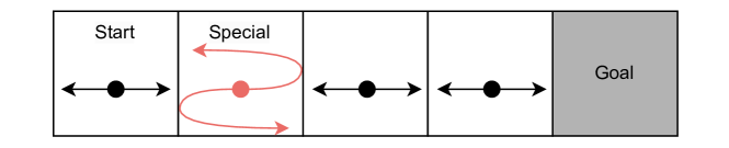
Figure 7. Long Corridor-5 environment, created according to the configuration shown in Table 3.

Long Corridor-5 environment - an image visualising the environment.

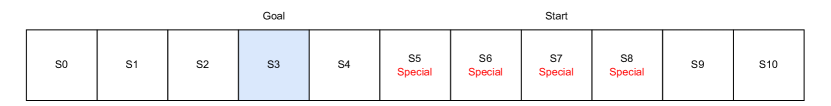
Figure 8. Long Corridor-11 environment, created according to the configuration shown in Table 3.

Long Corridor-11 environment - an image visualising the environment.

Table 3. Environment configurations for the three environments in Switcheroo Corridor Environment Set

Name (Short code)	Corridor Length	Start State	Goal State	Special State(s)
Small Corridor (SC)	4	0	3	[1]
Long Corridor-5 (LC-5)	5	0	4	[1]
Long Corridor-11 (LC-11)	11	7	3	[5, 6, 7, 8]

C.2. Blackjack

The Blackjack environment from (Sutton and Barto, 2018, Chapter 5.1) is a simplified version of the Blackjack card game. The standard Blackjack rules can be found at https://en.wikipedia.org/wiki/Blackjack. The environment terminates when the agent sticks or its hand exceeds 21, and termination never happens. It receives a reward of +1 for winning, -1 for losing and 0 for drawing.

Our experiments use the Gymnasium’s implementation at https://Gymnasium.farama.org/environments/toy_text/blackjack/. Instead of using Gymnasium’s tuple observation (the player’s current sum, the dealer’s hand, and the player’s useable ace), we convert each value to a one-hot encoding but in the range $\{-1,1\}$ and stack them together as the observation. There are 44 bits in total in the final observation encoding. The observation input to the neural DNF-MT actor is shown in Figure 2.

C.3. Taxi

The Taxi environment, purposed in Dietterich (2000), has 4 coloured squares where a hotel and the passenger will be allocated initially at the start. The hotel location remains unchanged throughout the episode. The agent controls a taxi to pick up the passenger and drop them off at the hotel. Each step gives a -1 reward, but illegally executing ‘pickup’ and ‘drop-off’ gives a -10 reward. If a passenger is successfully delivered to the hotel, the agent receives a +20 reward.

Our experiments use Gymnasium’s implementation at https://Gymnasium.farama.org/environments/toy_text/taxi/. By default, the truncation step limit is 200.

Figure 9. Taxi Environment: the taxi needs to pick up a passenger and drop them off at the destination hotel to finish the episode.

Taxi environment - an image visualising the environment.

C.4. Door Corridor

The Door Corridor environment (as shown in Figure 6) is a custom environment created based on the MiniGrid environment Chevalier-Boisvert et al. (2023). The implementation of the environment is based on Gymnasium’s MiniGrid. We keep the observation similar to MiniGrid’s style: a 3$\times$3 grid with two channels of objects and cell status. The agent receives a -1 reward for each step, and the default truncation step limit is 270.

⬇

1# Action space

2class DoorCorridorAction(IntEnum):

3 LEFT = 0

4 RIGHT = 1

5 FORWARD = 2

6 TOGGLE = 3

7

8# Observation space

9class Object(IntEnum):

10 UNSEEN = 0

11 EMPTY = 1

12 WALL = 2

13 DOOR = 3

14 AGENT = 4

15 GOAL = 5

16

17class State(IntEnum):

18 OPEN = 0 # Most objects will be OPEN

19 CLOSED = 1 # A door can be OPEN or CLOSED

Listing 7: Door Corridor Environment action space and observation space.

The two variants, Door Corridor-T (DC-T) and Door Corridor-OT (DC-OT), only differ in their termination check. DC-T terminates when the agent toggles the goal cell without being in it, and DC-OT terminates when the agent stands on the goal and then toggles.

Table 4 shows the optimal policy’s actions for the Door Corridor environment and its variants.

Table 4. Optimal policy’s actions for the Door Corridor (DC) environment and its variants, with blue text showing the difference in the variants.

Environment	Optimal policy’s actions (text)	Optimal policy’s actions (int)
DC	[Right, Toggle, Forward, Toggle, Forward, Toggle, Forward, Forward]	[1, 3, 2, 3, 2, 3, 2, 2]
DC-T	[Right, Toggle, Forward, Toggle, Forward, Toggle, Forward, Toggle]	[1, 3, 2, 3, 2, 3, 2, 3]
DC-OT	[Right, Toggle, Forward, Toggle, Forward, Toggle, Forward, Forward, Toggle]	[1, 3, 2, 3, 2, 3, 2, 2, 3]

Appendix D Additional Experimental Results

We use the clingo solver Potassco, the Potsdam Answer Set Solving Collection (2022) to run ASP programs.

Table 5 shows the performance of the models in all environments.

Table 5. Performance of the models in all environments, together with the logic programs extracted from their corresponding neural DNF-MT actors. The episodic return metric is represented in the form of mean $\pm$ standard error. For the Switcheroo Corridor environment set and Door Corridor environment, each model has 16 runs with different seeds. For Blackjack and Taxi environments, each model has 10 runs with different seeds. Each run is evaluated over 1,000,000 episodes and takes the average as the run’s performance. The final metric is calculated over the list of each run’s averaged episodic returns. All Q-tables are trained using Q-learning. Different symbols after the actor name indicate different action selection methods: * for argmax action selection, $\dagger$ for $\epsilon$-greedy sampling, and $\ddagger$ for actor’s distribution sampling.

Environment	Actor Model	Episodic return
SC MDP	Q-table*	-3.000 $\pm$ 0.000
	MLP*	-3.000 $\pm$ 0.000
	Neural DNF-MT*	-3.000 $\pm$ 0.000
	NDNF-MT: ASP*	-3.000 $\pm$ 0.000
SC POMDP	Q-table$\dagger$	-30.683 $\pm$ 0.006
	MLP$\ddagger$	-9.342 $\pm$ 0.022
	Neural DNF-MT$\ddagger$	-9.336 $\pm$ 0.019
	NDNF-MT: ProbLog$\ddagger$	-9.607 $\pm$ 0.129
LC-5 MDP	Q-table*	-4.000 $\pm$ 0.000
	MLP*	-4.000 $\pm$ 0.000
	Neural DNF-MT*	-4.000 $\pm$ 0.000
	NDNF-MT: ASP*	-4.000 $\pm$ 0.000
LC-5 POMDP	Q-table$\dagger$	-31.459 $\pm$ 0.004
	MLP$\ddagger$	-14.304 $\pm$ 0.047
	Neural DNF-MT$\ddagger$	-14.212 $\pm$ 0.031
	NDNF-MT: ProbLog$\ddagger$	-15.358 $\pm$ 0.193
LC-11 MDP	Q-table*	-4.000 $\pm$ 0.000
	MLP*	-4.000 $\pm$ 0.000
	Neural DNF-MT*	-4.000 $\pm$ 0.000
	NDNF-MT: ASP*	-4.000 $\pm$ 0.000
LC-11 POMDP	Q-table$\dagger$	-31.235 $\pm$ 0.004
	MLP$\ddagger$	-17.625 $\pm$ 0.051
	Neural DNF-MT$\ddagger$	-17.433 $\pm$ 0.056
	NDNF-MT: ProbLog$\ddagger$	-17.361 $\pm$ 0.183
Blackjack	Q-table Sutton and Barto (2018)*	-0.050 $\pm$ 0.001
	MLP*	-0.045 $\pm$ 0.000
	MLP$\ddagger$	-0.057 $\pm$ 0.001
	Neural DNF-MT*	-0.050 $\pm$ 0.001
	Neural DNF-MT$\ddagger$	-0.068 $\pm$ 0.001
	NDNF-MT: ProbLog$\ddagger$	-0.099 $\pm$ 0.007
Taxi	Q-table*	7.913 $\pm$ 0.009
	MLP*	7.865 $\pm$ 0.066
	MLP$\ddagger$	7.550 $\pm$ 0.011
	Neural DNF-MT*	7.926 $\pm$ 0.009
	Neural DNF-MT$\ddagger$	7.424 $\pm$ 0.009
	NDNF-MT: ProbLog$\ddagger$	7.604 $\pm$ 0.139
Door Corridor	MLP*	-8.000 $\pm$ 0.000
	Neural DNF-MT*	-8.000 $\pm$ 0.000
	NDNF-MT: ASP*	-8.000 $\pm$ 0.000

D.1. Switcheroo Corridor

The model architectures are listed below:

Model	Architecture
MLP actor MDP	(0): Linear(in=N_STATES, out=4, bias=True) (1): Tanh() (2): Linear(in=4, out=2, bias=True)
MLP actor POMDP	(0): Linear(in=2, out=4, bias=True) (1): Tanh() (2): Linear(in=4, out=2, bias=True)
NDNF-MT actor MDP	(0): SemiSymbolic(         in=N_STATES, out=4, type=CONJ.) (1): SemiSymbolicMutexTanh(         in=4, out=2, type=DISJ.)
NDNF-MT actor POMDP	(0): SemiSymbolic(         in=2, out=4, type=CONJ.) (1): SemiSymbolicMutexTanh(         in=4, out=2, type=DISJ.)
Critic MDP	(0): Linear(in=N_STATES, out=64, bias=True) (1): Tanh() (2): Linear(in=64, out=1, bias=True)
Critic POMDP	(0): Linear(in=2, out=64, bias=True) (1): Tanh() (2): Linear(in=64, out=1, bias=True)

The PPO hyperparameters used for training both the MLP actor and the neural DNF-MT actor are listed below:

Hyperparameter	Value
total_timesteps	$1\mathrm{e}{5}$
learning_rate	$1\mathrm{e}{-2}$
num_envs	8
num_steps	64
anneal_lr	True
gamma	0.99
gae_lambda	0.95
num_minibatches	8
update_epochs	4
norm_adv	True
clip_coef	0.3
clip_vloss	True
ent_coef	0.1
vf_coef	1
max_grad_norm	0.5

For the neural DNF-MT actor, the hyperparameters of the auxiliary losses and $\delta$ delay scheduling used are listed below:

Hyperparameter Group	Hyperparameter Name	Value
Auxiliary Loss	dis_weight_reg_lambda	0
	conj_tanh_out_reg_lambda	0
	mt_lambda	$1\mathrm{e}{-3}$
Delta Scheduling	initial_delta	0.1
	delta_decay_delay	30
	delta_decay_steps	5
	delta_decay_rate	1.1

We provide more interpretability examples for Long Corridor-5 (LC-5) and Long Corridor-11 (LC-11) environments in this section.

LC-5.  The special state is also at state 1. Listing 8 is the ASP program for a neural DNF-MT actor in LC-5 MDP, with correctly identifying the special state, state 1.

⬇

1action(left) :- in_s_1.

2action(right) :- not in_s_1.

Listing 8: ASP rules for a neural DNF-MT actor in LC-5 MDP.

Listing 9 is the ProbLog rules for one neural DNF-MT actor of the runs in LC-5 POMDP. Again, with wall status observations, the actor needs to be ‘flexible’ when there is no wall on either side, as shown in line 2 in Listing 9. The probability of going left and right differs from the SC POMDP case, as there is one more state with no walls on either side in LC5.

⬇

10.139::action(left) ; 0.861::action(right) :- left_wall_present, \+ right_wall_present.

20.326::action(left) ; 0.674::action(right) :- \+ left_wall_present, \+ right_wall_present.

Listing 9: ProbLog rules for a neural DNF-MT actor in LC-5 POMDP.

LC-11.  The special states are 5, 6, 7 and 8, while the agent needs to go from state 7 to state 3. The minimal path goes through $[7,6,5,4]$ in order, with action $[\text{right, right, right, left}]$.

Listing 10 is the ASP program for a neural DNF-MT actor in LC-11 MDP. It correctly captures the special states that it will go through in the minimal path in a single conjunction note (‘conj_3’ in line 3).

⬇

1action(left) :- conj_3.

2action(right) :- not conj_3.

3conj_3 :- not in_s_5, not in_s_6, not in_s_7.

Listing 10: ASP rules for a neural DNF-MT actor in LC-11 MDP.

Listing 11 is the ProbLog program for a neural DNF-MT actor in LC-11 POMDP. The left wall will never be present since the agent will never see the state 0. This is reflected in the ProbLog rules, where ‘left_wall_present’ is never considered. The agent prefers to go right when there is no right wall present. Under action sampling, there is a chance of the agent getting to state 11, where the right wall is present, as reflected in line 2. And we observe that the probability distribution in state 11 is not 0%-100% but 75.6%-24.4% (line 2). This is because the agent is not guaranteed to get to state 11 consistently, making the training less ‘balanced’ regarding state visiting frequency.

⬇

10.244::action(left) ; 0.756::action(right) :-

2 \+ right_wall_present.

30.756::action(left) ; 0.244::action(right) :-

4 right_wall_present.

Listing 11: ProbLog rules for a neural DNF-MT actor in LC-11 POMDP.

D.2. Blackjack

The model architectures are listed below:

Model	Architecture
MLP actor	(0): Linear(in=44, out=64, bias=True) (1): Tanh() (2): Linear(in=64, out=2, bias=True)
NDNF-MT actor	(0): SemiSymbolic(         in=44, out=64, type=CONJ.) (1): SemiSymbolicMutexTanh(         in=64, out=2, type=DISJ.)
Critic	(0): Linear(in=44, out=64, bias=True) (1): Tanh() (2): Linear(in=64, out=1, bias=True)

The PPO hyperparameters used for training both the MLP actor and the neural DNF-MT actor are listed below:

Hyperparameter	Value
total_timesteps	$3\mathrm{e}{5}$
learning_rate	$1\mathrm{e}{-3}$
num_envs	32
num_steps	16
anneal_lr	True
gamma	0.99
gae_lambda	0.95
num_minibatches	16
update_epochs	4
norm_adv	True
clip_coef	0.3
clip_vloss	True
ent_coef	0.1
vf_coef	1
max_grad_norm	0.5

For the neural DNF-MT actor, the hyperparameters of the auxiliary losses and $\delta$ delay scheduling used are listed below:

Hyperparameter Group	Hyperparameter Name	Value
Auxiliary Loss	dis_weight_reg_lambda	$1\mathrm{e}{-6}$
	conj_tanh_out_reg_lambda	0
	mt_lambda	$1\mathrm{e}{-3}$
Delta Scheduling	initial_delta	0.1
	delta_decay_delay	100
	delta_decay_steps	10
	delta_decay_rate	1.1

Figure 10 shows the policy grids of a neural DNF-MT actor trained in the Blackjack environment without any post-training processing, and Figure 11 shows its extracted ProbLog policy grid. In both figures, a red square indicates that the argmax action of the agent is different from the baseline Q-table from Sutton and Barto (2018). We see that the extracted ProbLog policy grid shows more errors (red squares) compared to the original neural DNF-MT actor without any post-training processing.

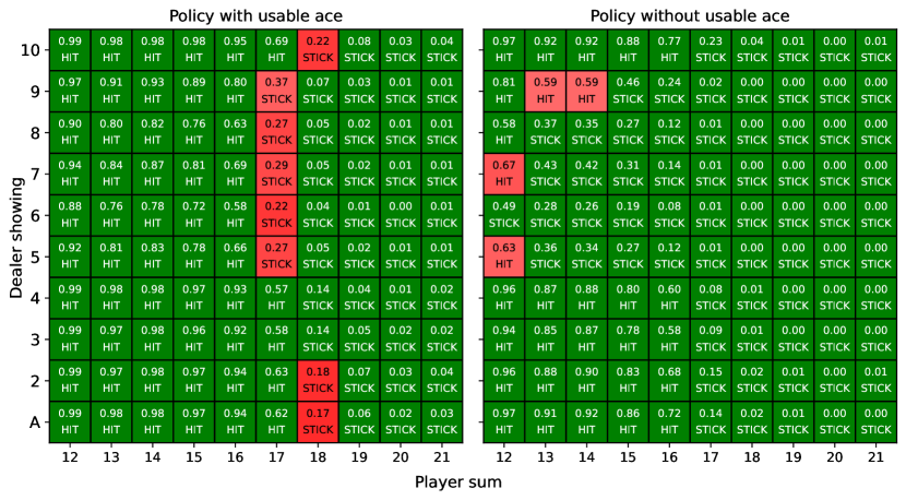
Figure 10. Policy grid of a neural DNF-MT actor in the Blackjack environment without post-training processing. Each square shows the probability of taking action ‘Hit’ and the argmax action in the text. If a square is red, it means that its argmax action is different from the baseline Q-table from Sutton and Barto (2018). The redder the square, the larger the probability difference.

Policy grid of a neural DNF-MT actor in the Blackjack environment without post-training processing.

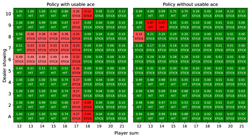
Figure 11. Extracted ProbLog policy grid of the same neural DNF-MT actor in Figure 10.

Extracted ProbLog policy grid of the same neural DNF-MT actor in Figure 10.

The neural DNF-MT actor’s ProbLog policy corresponding to Figure 11 is shown in Listing 12. The entire program contains 37 non-probabilistic rules with ‘conj_i’ as the rule head, and 201 annotated disjunctions with action probabilities.

⬇

10.873::action(stick) ; 0.127::action(hit) :- \+conj_3, \+conj_4, \+conj_5, \+conj_6, \+conj_7, \+conj_9, \+conj_10, \+conj_11, \+conj_12, \+conj_14, \+conj_15, \+conj_16, \+conj_19, \+conj_21, \+conj_22, \+conj_25, \+conj_29, \+conj_32, \+conj_34, \+conj_37, \+conj_40, \+conj_42, \+conj_44, \+conj_45, \+conj_47, \+conj_48, \+conj_49, \+conj_50, \+conj_51, \+conj_52, \+conj_53, \+conj_54, \+conj_55, \+conj_56, \+conj_57, \+conj_59, \+conj_62.

20.907::action(stick) ; 0.093::action(hit) :- \+conj_3, \+conj_4, \+conj_5, \+conj_6, \+conj_7, \+conj_9, \+conj_10, \+conj_11, \+conj_12, \+conj_14, \+conj_15, \+conj_16, \+conj_19, \+conj_21, \+conj_22, \+conj_25, \+conj_29, \+conj_32, \+conj_34, \+conj_37, \+conj_40, \+conj_42, \+conj_44, \+conj_45, \+conj_47, \+conj_48, \+conj_49, \+conj_50, \+conj_51, \+conj_52, \+conj_53, \+conj_54, conj_55, \+conj_56, \+conj_57, \+conj_59, \+conj_62.

30.900::action(stick) ; 0.100::action(hit) :- \+conj_3, \+conj_4, \+conj_5, \+conj_6, \+conj_7, \+conj_9, \+conj_10, \+conj_11, \+conj_12, \+conj_14, \+conj_15, \+conj_16, \+conj_19, \+conj_21, \+conj_22, \+conj_25, \+conj_29, \+conj_32, conj_34, \+conj_37, \+conj_40, \+conj_42, \+conj_44, \+conj_45, \+conj_47, \+conj_48, \+conj_49, \+conj_50, \+conj_51, \+conj_52, conj_53, \+conj_54, \+conj_55, \+conj_56, \+conj_57, \+conj_59, \+conj_62.

40.927::action(stick) ; 0.073::action(hit) :- \+conj_3, \+conj_4, \+conj_5, \+conj_6, \+conj_7, \+conj_9, \+conj_10, \+conj_11, \+conj_12, \+conj_14, \+conj_15, \+conj_16, \+conj_19, \+conj_21, \+conj_22, \+conj_25, \+conj_29, \+conj_32, conj_34, \+conj_37, \+conj_40, \+conj_42, \+conj_44, \+conj_45, \+conj_47, \+conj_48, \+conj_49, \+conj_50, \+conj_51, \+conj_52, conj_53, \+conj_54, conj_55, \+conj_56, \+conj_57, \+conj_59, \+conj_62.

50.983::action(stick) ; 0.017::action(hit) :- \+conj_3, \+conj_4, \+conj_5, \+conj_6, \+conj_7, \+conj_9, \+conj_10, \+conj_11, \+conj_12, \+conj_14, \+conj_15, \+conj_16, \+conj_19, \+conj_21, \+conj_22, \+conj_25, \+conj_29, \+conj_32, conj_34, \+conj_37, \+conj_40, \+conj_42, conj_44, \+conj_45, \+conj_47, \+conj_48, \+conj_49, \+conj_50, \+conj_51, \+conj_52, conj_53, \+conj_54, conj_55, \+conj_56, \+conj_57, \+conj_59, \+conj_62.

6...

7conj_3 :-

8 hand(18), \+dealer(9), \+dealer(10), \+usable_ace.

9conj_4 :-

10 \+hand(17), \+hand(18), \+hand(19), \+hand(20), \+hand(21), \+hand(22), \+hand(28).

11conj_5 :-

12 hand(20), \+dealer(1), \+dealer(9), \+dealer(10), \+usable_ace.

13conj_6 :-

14 hand(12), \+dealer(5), usable_ace.

15conj_7 :-

16 hand(10), \+dealer(2), \+dealer(3), \+dealer(4), \+dealer(6).

17...

Listing 12: ProbLog rules for the neural DNF-MT actor as shown in Figure 11, showing the first five annotated disjunctions and the first five conjunction rules.

D.3. Taxi

The model architectures are listed below:

Model	Architecture
MLP actor	(0): Linear(in=500, out=256, bias=True) (1): Tanh() (2): Linear(in=256, out=6, bias=True)
Critic	(0): Linear(in=500, out=256, bias=True) (1): ReLU() (2): Linear(in=256, out=256, bias=True) (3): ReLU() (4): Linear(in=256, out=1, bias=True)
MLP oracle (for distillation)	(0): Linear(in=500, out=256, bias=False) (1): Tanh() (2): Linear(in=256, out=6, bias=False)
NDNF-MT actor (distilled)	(0): SemiSymbolic(         in=500, out=64, type=CONJ.) (1): SemiSymbolicMutexTanh(         in=64, out=6, type=DISJ.)

The PPO hyperparameters used for training the MLP actor are listed below:

Hyperparameter	Value
total_timesteps	$3\mathrm{e}{6}$
learning_rate_actor	$2\mathrm{e}{-4}$
learning_rate_critic	$2\mathrm{e}{-3}$
num_envs	64
num_steps	2048
anneal_lr	True
gamma	0.999
gae_lambda	0.946
num_minibatches	128
update_epochs	8
norm_adv	True
clip_coef	0.2
clip_vloss	True
ent_coef	0.003
vf_coef	0.5
max_grad_norm	0.5

The distillation hyperparameters used for training neural DNF-MT actors are listed below:

Hyperparameter Group	Hyperparameter Name	Value
Distilaltion	batch_size	32
	epoch	5000
	learning_rate	$1\mathrm{e}{-4}$
Auxiliary Loss	dis_weight_reg_lambda	$1\mathrm{e}{-4}$
	conj_tanh_out_reg_lambda	$1\mathrm{e}{-5}$
	mt_lambda	$1\mathrm{e}{-4}$
Delta Scheduling	initial_delta	0.1
	delta_decay_delay	1000
	delta_decay_steps	100
	delta_decay_rate	1.1

We provide an example of a neural DNF-MT actor’s ProbLog rules in Listing 13.

⬇

10.595::action(down) ; 0.000::action(up) ; 0.000::action(right) ; 0.405::action(left) ; 0.000::action(pickup) ; 0.000::action(dropoff) :- \+conj_0, \+conj_1, \+conj_3, \+conj_4, conj_5, conj_6, \+conj_7, \+conj_8, \+conj_9, \+conj_11, \+conj_12, \+conj_13, \+conj_14, conj_15, \+conj_16, \+conj_18, \+conj_19, conj_20, conj_21, \+conj_22, conj_23, conj_24, \+conj_25, \+conj_26, conj_27, \+conj_28, \+conj_29, conj_30, \+conj_31, \+conj_33, \+conj_34, \+conj_35, \+conj_37, \+conj_38, \+conj_39, conj_40, \+conj_41, \+conj_42, \+conj_43, \+conj_44, \+conj_45, \+conj_46, \+conj_47, \+conj_48, \+conj_50, \+conj_51, \+conj_52, \+conj_55, \+conj_56, conj_57, \+conj_58, conj_60, \+conj_62, conj_63.

20.602::action(down) ; 0.000::action(up) ; 0.000::action(right) ; 0.398::action(left) ; 0.000::action(pickup) ; 0.000::action(dropoff) :- \+conj_0, \+conj_1, \+conj_3, \+conj_4, conj_5, conj_6, \+conj_7, \+conj_8, \+conj_9, \+conj_11, conj_12, \+conj_13, \+conj_14, conj_15, \+conj_16, \+conj_18, \+conj_19, conj_20, conj_21, \+conj_22, conj_23, conj_24, \+conj_25, \+conj_26, conj_27, \+conj_28, \+conj_29, conj_30, \+conj_31, \+conj_33, \+conj_34, \+conj_35, \+conj_37, \+conj_38, \+conj_39, conj_40, \+conj_41, \+conj_42, \+conj_43, \+conj_44, \+conj_45, \+conj_46, \+conj_47, \+conj_48, \+conj_50, \+conj_51, \+conj_52, \+conj_55, \+conj_56, conj_57, \+conj_58, conj_60, \+conj_62, conj_63.

30.963::action(down) ; 0.000::action(up) ; 0.000::action(right) ; 0.036::action(left) ; 0.000::action(pickup) ; 0.001::action(dropoff) :- \+conj_0, \+conj_1, \+conj_3, \+conj_4, conj_5, conj_6, \+conj_7, \+conj_8, \+conj_9, \+conj_11, conj_12, \+conj_13, \+conj_14, conj_15, \+conj_16, \+conj_18, \+conj_19, conj_20, conj_21, \+conj_22, conj_23, conj_24, \+conj_25, \+conj_26, conj_27, \+conj_28, \+conj_29, conj_30, \+conj_31, \+conj_33, \+conj_34, \+conj_35, \+conj_37, \+conj_38, \+conj_39, conj_40, \+conj_41, \+conj_42, \+conj_43, \+conj_44, \+conj_45, \+conj_46, \+conj_47, conj_48, \+conj_50, \+conj_51, \+conj_52, \+conj_55, \+conj_56, \+conj_57, \+conj_58, conj_60, \+conj_62, conj_63.

40.000::action(down) ; 0.000::action(up) ; 0.000::action(right) ; 0.000::action(left) ; 1.000::action(pickup) ; 0.000::action(dropoff) :- conj_0, conj_1, conj_3, conj_4, conj_5, conj_6, \+conj_7, \+conj_8, \+conj_9, conj_11, conj_12, \+conj_13, \+conj_14, conj_15, \+conj_16, \+conj_18, conj_19, conj_20, conj_21, \+conj_22, conj_23, conj_24, \+conj_25, \+conj_26, conj_27, conj_28, \+conj_29, \+conj_30, \+conj_31, \+conj_33, \+conj_34, \+conj_35, \+conj_37, \+conj_38, conj_39, \+conj_40, \+conj_41, \+conj_42, \+conj_43, conj_44, \+conj_45, \+conj_46, \+conj_47, conj_48, \+conj_50, \+conj_51, conj_52, \+conj_55, \+conj_56, conj_57, \+conj_58, conj_60, \+conj_62, conj_63.

50.000::action(down) ; 0.000::action(up) ; 0.000::action(right) ; 0.000::action(left) ; 0.000::action(pickup) ; 1.000::action(dropoff) :- \+conj_0, conj_1, conj_3, \+conj_4, \+conj_5, conj_6, \+conj_7, \+conj_8, \+conj_9, conj_11, conj_12, \+conj_13, \+conj_14, \+conj_15, \+conj_16, \+conj_18, \+conj_19, conj_20, \+conj_21, \+conj_22, conj_23, \+conj_24, \+conj_25, \+conj_26, conj_27, \+conj_28, conj_29, \+conj_30, \+conj_31, \+conj_33, \+conj_34, \+conj_35, \+conj_37, \+conj_38, conj_39, conj_40, \+conj_41, \+conj_42, \+conj_43, conj_44, \+conj_45, \+conj_46, \+conj_47, conj_48, \+conj_50, \+conj_51, \+conj_52, \+conj_55, \+conj_56, \+conj_57, \+conj_58, conj_60, \+conj_62, conj_63.

6...

7conj_0 :- \+state(4), \+state(9), \+state(11), \+state(14), \+state(16), \+state(24), \+state(26), \+state(28), \+state(33), \+state(52), \+state(54), \+state(59), \+state(61), \+state(68), \+state(72), \+state(76), \+state(78), \+state(79), \+state(81), \+state(82), \+state(89), \+state(94), \+state(96), \+state(97), \+state(104), \+state(107), \+state(112), \+state(113), \+state(114), \+state(128), \+state(129), \+state(131), \+state(134), \+state(139), \+state(152), \+state(159), \+state(162), \+state(171), \+state(176), \+state(178), \+state(182), \+state(189), \+state(191), \+state(193), \+state(194), \+state(279), \+state(311), \+state(379), \+state(394), \+state(443), \+state(479), \+state(489).

8conj_1 :- \+state(14), \+state(21), \+state(28), \+state(61), \+state(62), \+state(63), \+state(68), \+state(69), \+state(76), \+state(78), \+state(81), \+state(82), \+state(88), \+state(96), \+state(101), \+state(121), \+state(128), \+state(131), \+state(136), \+state(138), \+state(144), \+state(162), \+state(163), \+state(166), \+state(168), \+state(176), \+state(177), \+state(178), \+state(182), \+state(186), \+state(187), \+state(188), \+state(189), \+state(191), \+state(193), \+state(196), \+state(238), \+state(246), \+state(256), \+state(266), \+state(267), \+state(276), \+state(278), \+state(281), \+state(286), \+state(298), \+state(303), \+state(327), \+state(331), \+state(332), \+state(333), \+state(339), \+state(341), \+state(342), \+state(343), \+state(344), \+state(348), \+state(349), \+state(351), \+state(352), \+state(353), \+state(354), \+state(359), \+state(363), \+state(366), \+state(367), \+state(382), \+state(383), \+state(384), \+state(388), \+state(391), \+state(394), \+state(396), \+state(398), \+state(401), \+state(402), \+state(404), \+state(406), \+state(412), \+state(413), \+state(414), \+state(423), \+state(427), \+state(428), \+state(431), \+state(434), \+state(437), \+state(438), \+state(439), \+state(441), \+state(443), \+state(448), \+state(449), \+state(451), \+state(452), \+state(454), \+state(457), \+state(458), \+state(459), \+state(462), \+state(464), \+state(466), \+state(468), \+state(469), \+state(481), \+state(483), \+state(484), \+state(488), \+state(489), \+state(491), \+state(496), \+state(498).

9conj_3 :- \+state(6), \+state(11), \+state(14), \+state(17), \+state(24), \+state(27), \+state(28), \+state(32), \+state(33), \+state(38), \+state(51), \+state(52), \+state(54), \+state(58), \+state(59), \+state(61), \+state(68), \+state(72), \+state(76), \+state(78), \+state(79), \+state(81), \+state(88), \+state(91), \+state(93), \+state(94), \+state(96), \+state(104), \+state(107), \+state(114), \+state(117), \+state(128), \+state(129), \+state(131), \+state(132), \+state(133), \+state(134), \+state(139), \+state(152), \+state(156), \+state(159), \+state(162), \+state(169), \+state(171), \+state(173), \+state(176), \+state(178), \+state(182), \+state(183), \+state(189), \+state(191), \+state(192), \+state(193), \+state(194), \+state(199), \+state(211), \+state(293), \+state(294), \+state(308), \+state(309), \+state(311), \+state(318), \+state(379), \+state(392), \+state(393), \+state(394), \+state(414), \+state(436), \+state(439), \+state(452).

10conj_4 :- \+state(4), \+state(6), \+state(8), \+state(9), \+state(12), \+state(14), \+state(16), \+state(18), \+state(19), \+state(24), \+state(26), \+state(27), \+state(29), \+state(32), \+state(33), \+state(34), \+state(37), \+state(38), \+state(39), \+state(42), \+state(43), \+state(48), \+state(51), \+state(56), \+state(59), \+state(61), \+state(68), \+state(71), \+state(73), \+state(74), \+state(76), \+state(79), \+state(82), \+state(83), \+state(88), \+state(91), \+state(92), \+state(93), \+state(94), \+state(97), \+state(99), \+state(101), \+state(104), \+state(108), \+state(109), \+state(111), \+state(112), \+state(113), \+state(117), \+state(119), \+state(121), \+state(126), \+state(127), \+state(129), \+state(131), \+state(132), \+state(133), \+state(134), \+state(136), \+state(137), \+state(139), \+state(141), \+state(143), \+state(146), \+state(148), \+state(151), \+state(158), \+state(162), \+state(166), \+state(169), \+state(171), \+state(172), \+state(173), \+state(174), \+state(176), \+state(177), \+state(178), \+state(179), \+state(183), \+state(184), \+state(186), \+state(187), \+state(189), \+state(191), \+state(192), \+state(193), \+state(194), \+state(201), \+state(203), \+state(208), \+state(211), \+state(218), \+state(222), \+state(266), \+state(267), \+state(272), \+state(273), \+state(274), \+state(277), \+state(284), \+state(286), \+state(293), \+state(294), \+state(297), \+state(299), \+state(301), \+state(302), \+state(303), \+state(304), \+state(306), \+state(307), \+state(309), \+state(311), \+state(312), \+state(313), \+state(314), \+state(321), \+state(322), \+state(323), \+state(328), \+state(332), \+state(334), \+state(338), \+state(339), \+state(341), \+state(343), \+state(344), \+state(346), \+state(347), \+state(351), \+state(352), \+state(353), \+state(361), \+state(362), \+state(368), \+state(369), \+state(371), \+state(372), \+state(373), \+state(382), \+state(383), \+state(384), \+state(386), \+state(389), \+state(391), \+state(392), \+state(393), \+state(394), \+state(396), \+state(397), \+state(401), \+state(402), \+state(403), \+state(404), \+state(406), \+state(407), \+state(414), \+state(418), \+state(419), \+state(421), \+state(422), \+state(427), \+state(429), \+state(433), \+state(436), \+state(438), \+state(442), \+state(444), \+state(446), \+state(447), \+state(449), \+state(451), \+state(453), \+state(454), \+state(456), \+state(457), \+state(458), \+state(459), \+state(461), \+state(462), \+state(463), \+state(467), \+state(468), \+state(471), \+state(477), \+state(482), \+state(486), \+state(487), \+state(489), \+state(491), \+state(496), \+state(497), \+state(498).

11conj_5 :- \+state(16), \+state(97), \+state(123), \+state(136), \+state(479).

12...

Listing 13: ProbLog rules for a distilled neural DNF-MT actor in the Taxi environment, showing five annotated disjunctions and first five conjunction rules.

D.4. Door Corridor

The model architectures are listed below:

Model	Architecture
Feature Encoder	(0): Conv2d(2, 4, kernel_size=(1, 1), stride=(1, 1)) (1): Tanh() (2): Linear(in=36, out=16, bias=True)
MLP actor	(0): Linear(in=16, out=64, bias=True) (1): Tanh() (2): Linear(in=64, out=4, bias=True)
NDNF-MT Actor	(0): SemiSymbolic(         in=16, out=12, type=CONJ.) (1): SemiSymbolicMutexTanh(         in=12 out=4, type=DISJ.)
Critic	(0): Linear(in=16, out=64, bias=True) (1): Tanh() (2): Linear(in=64, out=1, bias=True)

The PPO hyperparameters used for training both the MLP actor and the neural DNF-MT actor are listed below:

Hyperparameter	Value
total_timesteps	$3\mathrm{e}{5}$
learning_rate	$1\mathrm{e}{-2}$
num_envs	8
num_steps	64
anneal_lr	True
gamma	0.99
gae_lambda	0.95
num_minibatches	8
update_epochs	4
norm_adv	True
clip_coef	0.3
clip_vloss	True
ent_coef	0.1
vf_coef	1
max_grad_norm	0.5

For the neural DNF-MT actor, the hyperparameters of the auxiliary losses and $\delta$ delay scheduling used are listed below:

Hyperparameter Group	Hyperparameter Name	Value
Auxiliary Loss	dis_weight_reg_lambda	0
	conj_tanh_out_reg_lambda	0
	mt_lambda	$1\mathrm{e}{-3}$
	embedding_reg_lambda	$3\mathrm{e}{-15}$
Delta Scheduling	initial_delta	0.1
	delta_decay_delay	50
	delta_decay_steps	10
	delta_decay_rate	1.1

The code repo provides a notebook on policy intervention in DC-T and DC-OT. The notebook’s path is notebooks/Door Corridor PPO NDNF-MT-6731 Intervention.ipynb (link to notebook).

Appendix E Run Time Comparison

Table 6 shows the run time comparison between different models in different environments. All entries are run on a 10-core Apple M1 Pro CPU with 16G RAM, and we use the ProbLog Python API to perform inference.

Table 6. Run time comparison between different models in different environments. The overall run time is the total time to run the model for the specified number of episodes. Models without * are run in a single environment in a loop for $n$ times. Models with * are run in 8 parallel environments for a total of $n$ episodes.

Env.	Model	No. episodes	Overall run time (s)	Avg. run time (s) per epidose
Blackjack	Q-table	$1\mathrm{e}{4}$	0.416	$4.156\mathrm{e}{-5}$
	MLP		2.283	$2.283\mathrm{e}{-4}$
	MLP*		1.157	$1.157\mathrm{e}{-4}$
	NDNF-MT		5.564	$5.564\mathrm{e}{-4}$
	NDNF-MT*		1.574	$1.574\mathrm{e}{-4}$
	ProbLog	10	21.583	$2.158$
Taxi	Q-table	$1\mathrm{e}{4}$	1.202	$1.202\mathrm{e}{-4}$
	MLP		17.338	$1.734\mathrm{e}{-3}$
	MLP*		7.279	$7.279\mathrm{e}{-4}$
	NDNF-MT		49.954	$4.995\mathrm{e}{-3}$
	NDNF-MT*		9.790	$9.790\mathrm{e}{-4}$
	ProbLog	1	Timed out after 30 min
Door Corridor	MLP	$1\mathrm{e}{4}$	10.178	$1.018\mathrm{e}{-3}$
	MLP*		0.073	$7.258\mathrm{e}{-6}$
	NDNF-MT		36.726	$3.673\mathrm{e}{-3}$
	NDNF-MT*		0.111	$1.112\mathrm{e}{-5}$
	ASP	1000	25.296	$2.530\mathrm{e}{-2}$

We also run an experiment to approximate the time taken to perform inference in ProbLog when the program is large. All programs are in the following form:

⬇

1p_0_1 :: action(0) ; ... ; p_0_n :: action(n) :- rule(0).

2p_1_1 :: action(0) ; ... ; p_1_n :: action(n) :- rule(1).

3...

4p_m_1 :: action(0) ; ... ; p_m_n :: action(n) :- rule(m).

We try with $n\in\{2,6\},m\in\{1..18\}$. The time taken is shown in Figure 12, and we observe the overall trend of exponential growth in time to the number of rules. This is only for approximation since the actual policy does not resemble the format we use here. A Problog program extracted from a neural DNF-MT actor in a Blackjack environment has 58 annotated disjunctions. It takes 2652.212s to perform 380 times of inference, averaging 7s per inference. Regardless, we can still conclude that inference with ProbLog is more expensive than with neural models.

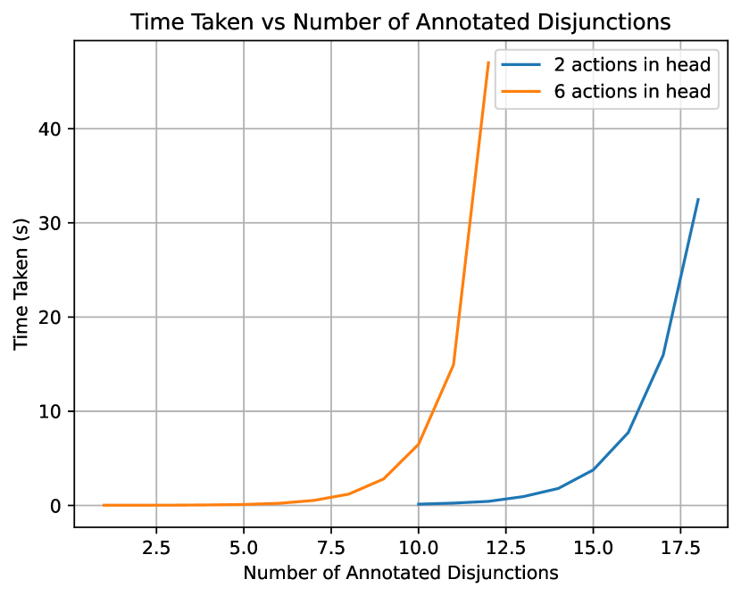
Figure 12. Time taken vs the number of annotated disjunctions in ProbLog, using a ProbLog program in a certain format as an approximation. The overall trend is that the time taken increases exponentially with the number of rules presented in the ProbLog program. However, we cannot confirm this pattern is the same as inference with an actual policy extracted from a neural DNF-MT actor.

Time taken vs number of annotated disjunctions in ProbLog.

References

- (1)
- ai- (2024) 2024. EU AI Act. https://artificialintelligenceact.eu/article/13/
- Ansel et al. (2024) Jason Ansel, Edward Yang, Horace He, Natalia Gimelshein, Animesh Jain, Michael Voznesensky, Bin Bao, Peter Bell, David Berard, Evgeni Burovski, Geeta Chauhan, Anjali Chourdia, Will Constable, Alban Desmaison, Zachary DeVito, Elias Ellison, Will Feng, Jiong Gong, Michael Gschwind, Brian Hirsh, Sherlock Huang, Kshiteej Kalambarkar, Laurent Kirsch, Michael Lazos, Mario Lezcano, Yanbo Liang, Jason Liang, Yinghai Lu, CK Luk, Bert Maher, Yunjie Pan, Christian Puhrsch, Matthias Reso, Mark Saroufim, Marcos Yukio Siraichi, Helen Suk, Michael Suo, Phil Tillet, Eikan Wang, Xiaodong Wang, William Wen, Shunting Zhang, Xu Zhao, Keren Zhou, Richard Zou, Ajit Mathews, Gregory Chanan, Peng Wu, and Soumith Chintala. 2024. PyTorch 2: Faster Machine Learning Through Dynamic Python Bytecode Transformation and Graph Compilation. In 29th ACM International Conference on Architectural Support for Programming Languages and Operating Systems, Volume 2 (ASPLOS ’24). ACM. https://doi.org/10.1145/3620665.3640366
- Baugh et al. (2023) Kexin Gu Baugh, Nuri Cingillioglu, and Alessandra Russo. 2023. Neuro-symbolic Rule Learning in Real-world Classification Tasks. In Proceedings of the AAAI 2023 Spring Symposium on Challenges Requiring the Combination of Machine Learning and Knowledge Engineering (AAAI-MAKE 2023), Andreas Martin, Hans-Georg Fill, Aurona Gerber, Knut Hinkelmann, Doug Lenat, Reinhard Stolle, and Frank van Harmelen (Eds.), Vol. Vol-3433. CEUR Workshop Proceedings. https://ceur-ws.org/Vol-3433/paper12.pdf
- Berner et al. (2019) Christopher Berner, Greg Brockman, Brooke Chan, Vicki Cheung, Przemyslaw Debiak, Christy Dennison, David Farhi, Quirin Fischer, Shariq Hashme, Christopher Hesse, Rafal Józefowicz, Scott Gray, Catherine Olsson, Jakub Pachocki, Michael Petrov, Henrique Pondé de Oliveira Pinto, Jonathan Raiman, Tim Salimans, Jeremy Schlatter, Jonas Schneider, Szymon Sidor, Ilya Sutskever, Jie Tang, Filip Wolski, and Susan Zhang. 2019. Dota 2 with Large Scale Deep Reinforcement Learning. CoRR abs/1912.06680 (2019). arXiv:1912.06680 http://arxiv.org/abs/1912.06680
- Cao et al. (2024) Yushi Cao, Zhiming Li, Tianpei Yang, Hao Zhang, Yan Zheng, Yi Li, Jianye Hao, and Yang Liu. 2024. GALOIS: boosting deep reinforcement learning via generalizable logic synthesis. In Proceedings of the 36th International Conference on Neural Information Processing Systems (New Orleans, LA, USA) (NIPS ’22). Curran Associates Inc., Red Hook, NY, USA, Article 1449, 14 pages.
- Chevalier-Boisvert et al. (2023) Maxime Chevalier-Boisvert, Bolun Dai, Mark Towers, Rodrigo de Lazcano, Lucas Willems, Salem Lahlou, Suman Pal, Pablo Samuel Castro, and Jordan Terry. 2023. Minigrid & Miniworld: Modular & Customizable Reinforcement Learning Environments for Goal-Oriented Tasks. CoRR abs/2306.13831 (2023).
- Cingillioglu and Russo (2021) Nuri Cingillioglu and Alessandra Russo. 2021. pix2rule: End-to-end Neuro-symbolic Rule Learning. In Proceedings of the 15th International Workshop on Neural-Symbolic Learning and Reasoning (NeSy 2021) as part of the 1st International Joint Conference on Learning & Reasoning (IJCLR 2021), Artur d’Avila Garcez and Ernesto Jiménez-Ruiz (Eds.). CEUR Workshop Proceedings. https://ceur-ws.org/Vol-2986/paper3.pdf
- Cropper et al. (2022) Andrew Cropper, Sebastijan Dumančić, Richard Evans, and Stephen H. Muggleton. 2022. Inductive logic programming at 30. Machine Learning 111, 1 (01 Jan 2022), 147–172. https://doi.org/10.1007/s10994-021-06089-1
- De Raedt et al. (2007) Luc De Raedt, Angelika Kimmig, and Hannu Toivonen. 2007. ProbLog: a probabilistic prolog and its application in link discovery. In Proceedings of the 20th International Joint Conference on Artifical Intelligence (Hyderabad, India) (IJCAI’07). Morgan Kaufmann Publishers Inc., San Francisco, CA, USA, 2468–2473.
- Delfosse et al. (2023) Quentin Delfosse, Hikaru Shindo, Devendra Dhami, and Kristian Kersting. 2023. Interpretable and Explainable Logical Policies via Neurally Guided Symbolic Abstraction. In Advances in Neural Information Processing Systems, A. Oh, T. Naumann, A. Globerson, K. Saenko, M. Hardt, and S. Levine (Eds.), Vol. 36. Curran Associates, Inc., 50838–50858. https://proceedings.neurips.cc/paper_files/paper/2023/file/9f42f06a54ce3b709ad78d34c73e4363-Paper-Conference.pdf
- Dietterich (2000) Thomas G Dietterich. 2000. Hierarchical reinforcement learning with the MAXQ value function decomposition. Journal of artificial intelligence research 13 (2000), 227–303.
- Dong et al. (2019) Honghua Dong, Jiayuan Mao, Tian Lin, Chong Wang, Lihong Li, and Denny Zhou. 2019. Neural Logic Machines. In 7th International Conference on Learning Representations, ICLR 2019, New Orleans, LA, USA, May 6-9, 2019. OpenReview.net. https://openreview.net/forum?id=B1xY-hRctX
- Džeroski et al. (2001) Sašo Džeroski, Luc De Raedt, and Kurt Driessens. 2001. Relational Reinforcement Learning. Machine Learning 43, 1 (01 Apr 2001), 7–52. https://doi.org/10.1023/A:1007694015589
- Evans and Grefenstette (2018) Richard Evans and Edward Grefenstette. 2018. Learning explanatory rules from noisy data. Journal of Artificial Intelligence Research 61 (2018), 1–64.
- Gao et al. (2020) Xiaojie Gao, Yueming Jin, Qi Dou, and Pheng-Ann Heng. 2020. Automatic Gesture Recognition in Robot-assisted Surgery with Reinforcement Learning and Tree Search. In 2020 IEEE International Conference on Robotics and Automation (ICRA). 8440–8446. https://doi.org/10.1109/ICRA40945.2020.9196674
- He et al. (2019) Jianxing He, Sally L. Baxter, Jie Xu, Jiming Xu, Xingtao Zhou, and Kang Zhang. 2019. The practical implementation of artificial intelligence technologies in medicine. Nature Medicine 25, 1 (01 Jan 2019), 30–36. https://doi.org/10.1038/s41591-018-0307-0
- Huang et al. (2022) Shengyi Huang, Rousslan Fernand Julien Dossa, Chang Ye, Jeff Braga, Dipam Chakraborty, Kinal Mehta, and João G.M. Araújo. 2022. CleanRL: High-quality Single-file Implementations of Deep Reinforcement Learning Algorithms. Journal of Machine Learning Research 23, 274 (2022), 1–18. http://jmlr.org/papers/v23/21-1342.html
- Jiang and Luo (2019) Zhengyao Jiang and Shan Luo. 2019. Neural Logic Reinforcement Learning. In Proceedings of the 36th International Conference on Machine Learning (Proceedings of Machine Learning Research, Vol. 97), Kamalika Chaudhuri and Ruslan Salakhutdinov (Eds.). PMLR, 3110–3119. https://proceedings.mlr.press/v97/jiang19a.html
- Kaelbling et al. (1998) Leslie Pack Kaelbling, Michael L. Littman, and Anthony R. Cassandra. 1998. Planning and acting in partially observable stochastic domains. Artificial Intelligence 101, 1 (1998), 99–134. https://doi.org/10.1016/S0004-3702(98)00023-X
- Kimura et al. (2021) Daiki Kimura, Masaki Ono, Subhajit Chaudhury, Ryosuke Kohita, Akifumi Wachi, Don Joven Agravante, Michiaki Tatsubori, Asim Munawar, and Alexander Gray. 2021. Neuro-Symbolic Reinforcement Learning with First-Order Logic. In Proceedings of the 2021 Conference on Empirical Methods in Natural Language Processing, Marie-Francine Moens, Xuanjing Huang, Lucia Specia, and Scott Wen-tau Yih (Eds.). Association for Computational Linguistics, Online and Punta Cana, Dominican Republic, 3505–3511. https://doi.org/10.18653/v1/2021.emnlp-main.283
- Lifschitz (2019) Vladimir Lifschitz. 2019. Answer set programming. Springer Nature, Cham, Switzerland. https://doi.org/10.1007/978-3-030-24658-7
- Mnih et al. (2016) Volodymyr Mnih, Adria Puigdomenech Badia, Mehdi Mirza, Alex Graves, Timothy Lillicrap, Tim Harley, David Silver, and Koray Kavukcuoglu. 2016. Asynchronous Methods for Deep Reinforcement Learning. In Proceedings of The 33rd International Conference on Machine Learning (Proceedings of Machine Learning Research, Vol. 48), Maria Florina Balcan and Kilian Q. Weinberger (Eds.). PMLR, New York, New York, USA, 1928–1937. https://proceedings.mlr.press/v48/mniha16.html
- Mnih et al. (2015) Volodymyr Mnih, Koray Kavukcuoglu, David Silver, Andrei A. Rusu, Joel Veness, Marc G. Bellemare, Alex Graves, Martin Riedmiller, Andreas K. Fidjeland, Georg Ostrovski, Stig Petersen, Charles Beattie, Amir Sadik, Ioannis Antonoglou, Helen King, Dharshan Kumaran, Daan Wierstra, Shane Legg, and Demis Hassabis. 2015. Human-level control through deep reinforcement learning. Nature 518, 7540 (01 Feb 2015), 529–533. https://doi.org/10.1038/nature14236
- Muggleton (1995) Stephen Muggleton. 1995. Inverse entailment and progol. New Generation Computing 13, 3 (01 Dec 1995), 245–286. https://doi.org/10.1007/BF03037227
- Muggleton and de Raedt (1994) Stephen Muggleton and Luc de Raedt. 1994. Inductive Logic Programming: Theory and methods. The Journal of Logic Programming 19-20 (1994), 629–679. https://doi.org/10.1016/0743-1066(94)90035-3 Special Issue: Ten Years of Logic Programming.
- Potassco, the Potsdam Answer Set Solving Collection (2022) Potassco, the Potsdam Answer Set Solving Collection. 2022. Clingo: A grounder and solver for logic programs. University of Potsdam. https://github.com/potassco/clingo
- Puterman (1990) Martin L. Puterman. 1990. Markov decision processes. In Stochastic Models. Handbooks in Operations Research and Management Science, Vol. 2. Elsevier, 331–434. https://doi.org/10.1016/S0927-0507(05)80172-0
- Riegel et al. (2020) Ryan Riegel, Alexander G. Gray, Francois P. S. Luus, Naweed Khan, Ndivhuwo Makondo, Ismail Yunus Akhalwaya, Haifeng Qian, Ronald Fagin, Francisco Barahona, Udit Sharma, Shajith Ikbal, Hima Karanam, Sumit Neelam, Ankita Likhyani, and Santosh K. Srivastava. 2020. Logical Neural Networks. CoRR abs/2006.13155 (2020). arXiv:2006.13155 https://arxiv.org/abs/2006.13155
- Rudin (2019) Cynthia Rudin. 2019. Stop explaining black box machine learning models for high stakes decisions and use interpretable models instead. Nature Machine Intelligence 1, 5 (01 May 2019), 206–215. https://doi.org/10.1038/s42256-019-0048-x
- Schulman et al. (2017) John Schulman, Filip Wolski, Prafulla Dhariwal, Alec Radford, and Oleg Klimov. 2017. Proximal Policy Optimization Algorithms. CoRR abs/1707.06347 (2017). arXiv:1707.06347 http://arxiv.org/abs/1707.06347
- Shindo et al. (2021) Hikaru Shindo, Masaaki Nishino, and Akihiro Yamamoto. 2021. Differentiable inductive logic programming for structured examples. In Proceedings of the AAAI Conference on Artificial Intelligence, Vol. 35. 5034–5041.
- Silver et al. (2017) David Silver, Julian Schrittwieser, Karen Simonyan, Ioannis Antonoglou, Aja Huang, Arthur Guez, Thomas Hubert, Lucas Baker, Matthew Lai, Adrian Bolton, Yutian Chen, Timothy Lillicrap, Fan Hui, Laurent Sifre, George van den Driessche, Thore Graepel, and Demis Hassabis. 2017. Mastering the game of Go without human knowledge. Nature 550, 7676 (01 Oct 2017), 354–359. https://doi.org/10.1038/nature24270
- Sutton and Barto (2018) Richard S. Sutton and Andrew G. Barto. 2018. Reinforcement Learning: An Introduction. A Bradford Book, Cambridge, MA, USA.
- Towers et al. (2024) Mark Towers, Ariel Kwiatkowski, Jordan K Terry, John U. Balis, Gianluca de Cola, Tristan Deleu, Manuel Goulão, Andreas Kallinteris, Markus Krimmel, Arjun KG, Rodrigo Perez-Vicente, Andrea Pierré, Sander Schulhoff, Jun Jet Tai, Hannah Jin Shen Tan, and Omar G. Younis. 2024. Gymnasium: A Standard Interface for Reinforcement Learning Environments. Farama Foundation. https://github.com/Farama-Foundation/Gymnasium
- Verma et al. (2019) Abhinav Verma, Hoang M. Le, Yisong Yue, and Swarat Chaudhuri. 2019. Imitation-projected programmatic reinforcement learning. In Proceedings of the 33rd International Conference on Neural Information Processing Systems. Curran Associates Inc., Red Hook, NY, USA, Article 1411, 12 pages. https://proceedings.neurips.cc/paper_files/paper/2019/file/5a44a53b7d26bb1e54c05222f186dcfb-Paper.pdf
- Verma et al. (2018) Abhinav Verma, Vijayaraghavan Murali, Rishabh Singh, Pushmeet Kohli, and Swarat Chaudhuri. 2018. Programmatically Interpretable Reinforcement Learning. In Proceedings of the 35th International Conference on Machine Learning (Proceedings of Machine Learning Research, Vol. 80), Jennifer Dy and Andreas Krause (Eds.). PMLR, 5045–5054. https://proceedings.mlr.press/v80/verma18a.html
- Watkins and Dayan (1992) Christopher J. C. H. Watkins and Peter Dayan. 1992. Q-learning. Machine Learning 8, 3 (01 May 1992), 279–292. https://doi.org/10.1007/BF00992698
- Williams (1992) Ronald J. Williams. 1992. Simple Statistical Gradient-Following Algorithms for Connectionist Reinforcement Learning. Mach. Learn. 8, 3–4 (May 1992), 229–256. https://doi.org/10.1007/BF00992696
- Wu et al. (2023) XiaoDan Wu, RuiChang Li, Zhen He, TianZhi Yu, and ChangQing Cheng. 2023. A value-based deep reinforcement learning model with human expertise in optimal treatment of sepsis. npj Digital Medicine 6, 1 (02 Feb 2023), 15. https://doi.org/10.1038/s41746-023-00755-5
- Zambaldi et al. (2018) Vinícius Flores Zambaldi, David Raposo, Adam Santoro, Victor Bapst, Yujia Li, Igor Babuschkin, Karl Tuyls, David P. Reichert, Timothy P. Lillicrap, Edward Lockhart, Murray Shanahan, Victoria Langston, Razvan Pascanu, Matthew M. Botvinick, Oriol Vinyals, and Peter W. Battaglia. 2018. Relational Deep Reinforcement Learning. CoRR abs/1806.01830 (2018). arXiv:1806.01830 http://arxiv.org/abs/1806.01830
- Zimmer et al. (2021) Matthieu Zimmer, Xuening Feng, Claire Glanois, Zhaohui Jiang, Jianyi Zhang, Paul Weng, Jianye Hao, Dong Li, and Wulong Liu. 2021. Differentiable Logic Machines. CoRR abs/2102.11529 (2021). arXiv:2102.11529 https://arxiv.org/abs/2102.11529
- Åström (1965) K.J Åström. 1965. Optimal control of Markov processes with incomplete state information. J. Math. Anal. Appl. 10, 1 (1965), 174–205. https://doi.org/10.1016/0022-247X(65)90154-X