Spline Quantile Regression

Abstract

Quantile regression is a powerful tool capable of offering a richer view of the data as compared to linear-squares regression. Quantile regression is typically performed individually on a few quantiles or a grid of quantiles without considering the similarity of the underlying regression coefficients at nearby quantiles. When needed, an ad hoc post-processing procedure such as kernel smoothing is employed to smooth the estimated coefficients across quantiles and thereby improve the performance of these estimates. This paper introduces a new method, called spline quantile regression (SQR), that unifies quantile regression with quantile smoothing and jointly estimates the regression coefficients across quantiles as smoothing splines. We discuss the computation of the SQR solution as a linear program (LP) using an interior-point algorithm. We also experiment with some gradient algorithms that require less memory than the LP algorithm. The performance of the SQR method and these algorithms is evaluated using simulated and real-world data.

Keywords: function estimation, gradient descent, interior point, linear program, quantile periodogram, quantile regression, smoothing, spline

Acknowledgment: The authors would like to thank Dr. R. Koenker for advice on the FORTRAN code of the interior-point algorithm.

1 Introduction

Quantile regression (QR) is a powerful statistical tool that complements the conventional least-squares regression (Koenker and Bassett 1978; Koenker 2005). Quantile regression postulates the conditional quantile of a dependent variable, rather than the conditional mean, as a function of the explanatory variables. By varying the quantile level, one can explore this relationship across all quantiles and thereby obtains a richer view of the data than that offered by least-squares regression. Recent years have witnessed further development of the quantile regression method, Examples include, just to name a few, the fast algorithms to compute quantile regression when the number of regressors is very large (He et al. 2023), the statistical analyses for the regression coefficients as functions of the quantile level (Belloni et al. 2019; Hao et al. 2023), and the techniques to overcome quantile crossings for applications that require the quantiles to be monotone at any point in the space of regressors (He 1997; Wu and Liu 2009; Bondell et al. 2010).

In this paper, we are interested in situations where the underlying quantile regression coefficients vary smoothly across quantiles. In typical applications, the smoothness is either ignored entirely by performing quantile regression independently at different quantiles, or handled separately by employing an ad hoc post-processing procedure such as kernel smoothing to smooth the raw estimates across quantiles (Koenker 2005, pp. 158–159).

We offer an alternative solution, called spline quantile regression (SQR). The SQR method extends the original QR problem at an individual quantile into a function estimation problem across all quatiles. In this problem, the regression coefficients are treated as smooth functions of the quantile level in a space of splines, and the resulting model is fitted to the data jointly on a grid of quantiles. A penalty term is added to the QR cost function to regularize the smoothness of the functional regression coefficients. The SQR method unifies quantile regression with quantile smoothing and provides an estimator of regression coefficients as smoothing splines.

Smoothing splines have been used in the context of quantile regression to represent nonparametric regression functions (Koenker et al. 1994; Oh et al. 2011; Andriyana et al. 2014; He et al. 2021). In these methods, the smoothness of the regression function is regularized in a way similar to the spline smoothing problem under the least-squares framework (Wahba 1975). The SQR problem, on the other hand, represents the regression coefficients as spline functions of the quantile level. The resulting model is a linear function of the regressors for fixed quantile level, and a nonlinear smooth function of the quantile level for fixed regressors.

To retain the numerical characteristics of quantile regression, we employ the integral of the $L_{1}$-norm of second derivatives as the penalty to regularize the functional regression coefficients. A similar measure was employed in Koenker et al. (1994) for nonparametric quantile regression. We show that the resulting SQR problem can be reformulated as a primal-dual pair of linear program (LP) and solved using an interior-point algorithm developed by Portnoy and Koenker (1997) for the ordinary QR problem.

In this paper, we also experiment with some gradient algorithms as computationally more efficient alternatives to approximate the LP solution. This investigation is largely motivated by the success of gradient algorithms in training neural network models with non-smooth objective functions (Goodfellow et al. 2016; Ruder 2016). The success stories have generated renewed interest in trying to better understand the behavior of gradient algorithms in non-smooth situations (e.g., Lewis and Overton 2013; Asl and Overton 2020). As in machine learning applications, our aim is not to use these algorithms as a replacement of LP to produce the exact solution. Instead, we are interested in algorithms that provide sufficiently good approximations to the LP solution but with reduced computational burden, especially the demand on computer memory.

The remainder is organized as follows. Section 2 describes the SQR problem. Section 3 discusses the LP reformulation and proves the suitability of the interior-point algorithm. Section 4 presents some numerical examples with simulated and real-word data to demonstrate the SQR method. Section 5 describes the BFGS, ADAM, and GRAD algorithms. Section 6 contains the experimental results of gradient algorithms. Concluding remarks are given in Section 7. The R functions that implement the SQR method are described in Appendix.

2 Spline Quantile Regression

Let $\{y_{t}:t=1,\dots,n\}$ be a sequence of $n$ observations of a dependent variable and $\{\mathbf{x}_{t}:t=1,\dots,n\}$ be the corresponding values of a $p$-dimensional regressor. Given an increasing sequence of quantile levels $\{\tau_{\ell}:\ell=1,\dots,L\}\subset(0,1)$, the spline quantile regression (SQR) problem can be stated as

$$\hat{\boldsymbol{\beta}}(\cdot):=\operatorname*{argmin}_{\boldsymbol{\beta}(\cdot)\in\mathcal{F}^{p}}\bigg{\{}n^{-1}\sum_{\ell=1}^{L}\sum_{t=1}^{n}\rho_{\tau_{\ell}}(y_{t}-\mathbf{x}_{t}^{T}\boldsymbol{\beta}(\tau_{\ell}))+c\sum_{\ell=1}^{L}w_{\ell}\,\|\ddot{\boldsymbol{\beta}}(\tau_{\ell})\|_{1}\bigg{\}},$$ (1)

where $\mathcal{F}$ is a functional space spanned by spline basis functions, $\rho_{\tau}(y):=y(\tau-{\cal I}(y<0))$ is the objective function of quantile regression at quantile level $\tau$ (Koenker 2005, p. 5), $c\geq 0$ is a smoothing or penalty parameter, and $\{w_{\ell}\}$ is a sequence of nonnegative constants.

The $L_{1}$-norm of second derivatives is employed in (1) as the roughness measure of $\boldsymbol{\beta}(\cdot)$ in order to retain the LP characteristics of the original QR problem (Koenker 2005). The squared $L_{2}$-norm, which is commonly used for spline smoothing under the least-squares framework (Wahba 1975), is a possible alternative. This $L_{2}$-norm penalty would result in a quadratic program. We choose not to deal with the quadratic program in this paper. The weight sequence $\{w_{\ell}\}$ is introduced in (1) to allow different contributions from different quantiles to the penalty term. For example, taking $w_{\ell}:=0.25/(\tau_{\ell}(1-\tau_{\ell}))$ would limit the influence from high and low tails for their excessive statistical variability.

Let $\{\phi_{k}(\tau):k=1,\dots,K\}$ denote a set of spline basis functions of $\tau\in(0,1)$. Then, any function $\beta_{j}(\tau)$ in $\mathcal{F}$ can be expressed as

$$\beta_{j}(\tau)=\sum_{k=1}^{K}\phi_{k}(\tau)\theta_{jk}=\boldsymbol{\phi}^{T}(\tau){\boldsymbol{\theta}}_{j}\quad(j=1,\dots,p),$$

where

$$\boldsymbol{\phi}(\tau):=[\phi_{1}(\tau),\dots,\phi_{K}(\tau)]^{T}\in\mathbb{R}^{K},\quad{\boldsymbol{\theta}}_{j}\ :=[\theta_{j1},\dots,\theta_{jK}]^{T}\in\mathbb{R}^{K}.$$

Therefore, for any $\boldsymbol{\beta}(\tau):=[\beta_{1}(\tau),\dots,\beta_{p}(\tau)]^{T}\in\mathcal{F}^{p}$, we can write

$$\boldsymbol{\beta}(\tau)=\boldsymbol{\Phi}(\tau){\boldsymbol{\theta}},$$

where

$$\boldsymbol{\Phi}(\tau):=\mathbf{I}_{p}\otimes\boldsymbol{\phi}^{T}(\tau)\in\mathbb{R}^{p\times pK},\quad{\boldsymbol{\theta}}:=[{\boldsymbol{\theta}}_{1}^{T},\dots,{\boldsymbol{\theta}}_{p}^{T}]^{T}\in\mathbb{R}^{pK}.$$

With this notation and $c_{\ell}:=ncw_{\ell}$, the SQR problem (1) can be restated as

$$\hat{{\boldsymbol{\theta}}}:=\operatorname*{argmin}_{{\boldsymbol{\theta}}\in\mathbb{R}^{pK}}\bigg{\{}\sum_{\ell=1}^{L}\sum_{t=1}^{n}\rho_{\tau_{\ell}}(y_{t}-\mathbf{x}_{t}^{T}\boldsymbol{\Phi}(\tau_{\ell}){\boldsymbol{\theta}})+\sum_{\ell=1}^{L}c_{\ell}\,\|\ddot{\boldsymbol{\Phi}}(\tau_{\ell}){\boldsymbol{\theta}}\|_{1}\bigg{\}}$$ (2)

and

$$\hat{\boldsymbol{\beta}}(\tau):=\boldsymbol{\Phi}(\tau)\hat{{\boldsymbol{\theta}}}.$$ (3)

In other words, the SQR problem (1) can be solved by searching for the vector $\hat{{\boldsymbol{\theta}}}$ in $\mathbb{R}^{pK}$ according to (2) and then converting it to the desired function $\hat{\boldsymbol{\beta}}(\cdot)$ according to (3).

Note that the SQR problem is different from the problem of quantile smoothing splines considered by Koenker et al. (1994). The latter uses splines to represent nonparametric functions of independent variables. The SQR problem is also different from the problem considered by Andriyana et al. (2014) in which splines are used to represent regression coefficients as functions of time rather than the quantile level.

3 Linear Program Reformulation

Like the ordinary QR problem (Koenker 2005, p. 7), the SQR problem in (2) can be reformulated as a linear program (LP) with nonnegative decision variables:

$$(\hat{\boldsymbol{\gamma}},\hat{\boldsymbol{\delta}},\hat{\mathbf{u}}_{1},\hat{\mathbf{v}}_{1},\hat{\mathbf{r}}_{1},\hat{\mathbf{s}}_{1},\dots,\hat{\mathbf{u}}_{L},\hat{\mathbf{v}}_{L},\hat{\mathbf{r}}_{L},\hat{\mathbf{s}}_{L}):=$$ (6)

$$\operatorname*{argmin}_{(\boldsymbol{\gamma},\boldsymbol{\delta},\mathbf{u}_{1},\mathbf{v}_{1},\mathbf{r}_{1},\mathbf{s}_{1},\dots,\mathbf{u}_{L},\mathbf{v}_{L},\mathbf{r}_{L},\mathbf{s}_{L})\in\mathbb{R}_{+}^{d}}\ \sum_{\ell=1}^{L}\{\tau_{\ell}{\bf 1}_{n}^{T}\mathbf{u}_{\ell}+(1-\tau_{\ell}){\bf 1}_{n}^{T}\mathbf{v}_{\ell}+{\bf 1}_{p}^{T}\mathbf{r}_{\ell}+{\bf 1}_{p}^{T}\mathbf{s}_{\ell}\}$$

$$\quad{\rm s.t.}\quad\left\{\begin{array}[]{l}\mathbf{X}\,\boldsymbol{\Phi}(\tau_{\ell})(\boldsymbol{\gamma}-\boldsymbol{\delta})+\mathbf{u}_{\ell}-\mathbf{v}_{\ell}=\mathbf{y}\quad(\ell=1,\dots,L),\\ c_{\ell}\,\ddot{\boldsymbol{\Phi}}(\tau_{\ell})(\boldsymbol{\gamma}-\boldsymbol{\delta})-(\mathbf{r}_{\ell}-\mathbf{s}_{\ell})={\bf 0}\quad(\ell=1,\dots,L),\end{array}\right.$$

where ${\bf 1}_{n}$ and ${\bf 1}_{p}$ are the $n$-dimensional and $p$-dimensional vectors of 1’s, $\mathbf{X}:=[\mathbf{x}_{1},\dots,\mathbf{x}_{n}]^{T}$ is the regression design matrix, and $d:=2pK+2nL+2pL$ is the total number of decision variables to be optimized. Among the decision variables in (6), $\boldsymbol{\gamma}\in\mathbb{R}_{+}^{pK}$ and $\boldsymbol{\delta}\in\mathbb{R}_{+}^{pK}$ are primary variables which determine the solution $\hat{{\boldsymbol{\theta}}}$ in (2) such that

$$\hat{{\boldsymbol{\theta}}}=\hat{\boldsymbol{\gamma}}-\hat{\boldsymbol{\delta}}.$$ (7)

The remaining variables $\mathbf{u}_{\ell}\in\mathbb{R}_{+}^{n}$, $\mathbf{v}_{\ell}\in\mathbb{R}_{+}^{n}$, $\mathbf{r}_{\ell}\in\mathbb{R}_{+}^{p}$, and $\mathbf{s}_{\ell}\in\mathbb{R}_{+}^{p}$ are auxiliary variables introduced just for the purpose of linearizing the objective function in (2).

In the canonical form, the LP problem (6) can be expressed as

$$\min\{\mathbf{c}^{T}\boldsymbol{\xi}|\mathbf{A}\boldsymbol{\xi}=\mathbf{b};\boldsymbol{\xi}\in\mathbb{R}_{+}^{2pK+2nL+2pL}\},$$ (8)

where

$$\mathbf{c}:=[{\bf 0}_{p}^{T},{\bf 0}_{p}^{T},\tau_{1}{\bf 1}_{n}^{T},(1-\tau_{1}){\bf 1}_{n}^{T},{\bf 1}_{p}^{T},{\bf 1}_{p}^{T},\dots,\tau_{L}{\bf 1}_{n}^{T},(1-\tau_{L}){\bf 1}_{n}^{T},{\bf 1}_{p}^{T},{\bf 1}_{p}^{T}]^{T},$$

$$\boldsymbol{\xi}:=[\boldsymbol{\gamma}^{T},\boldsymbol{\delta}^{T},\mathbf{u}_{1}^{T},\mathbf{v}_{1}^{T},\mathbf{r}_{1}^{T},\mathbf{s}_{1}^{T},\dots,\mathbf{u}_{L}^{T},\mathbf{v}_{L}^{T},\mathbf{r}_{L}^{T},\mathbf{s}_{L}^{T}]^{T},$$

$$\mathbf{A}:=\left[\begin{array}[]{ccccccccccccc}\mathbf{X}\,\boldsymbol{\Phi}(\tau_{1})&-\mathbf{X}\,\boldsymbol{\Phi}(\tau_{1})&\mathbf{I}_{n}&-\mathbf{I}_{n}&{\bf 0}&{\bf 0}&\\ \vdots&\vdots&&&&&\ddots\\ \mathbf{X}\,\boldsymbol{\Phi}(\tau_{L})&-\mathbf{X}\,\boldsymbol{\Phi}(\tau_{L})&&&&&&\mathbf{I}_{n}&-\mathbf{I}_{n}&{\bf 0}&{\bf 0}\\ c_{1}\,\ddot{\boldsymbol{\Phi}}(\tau_{1})&-c_{1}\,\ddot{\boldsymbol{\Phi}}(\tau_{1})&{\bf 0}&{\bf 0}&\mathbf{I}_{p}&\mathbf{I}_{p}&\\ \vdots&\vdots&&&&&\ddots\\ c_{L}\,\ddot{\boldsymbol{\Phi}}(\tau_{L})&-c_{L}\,\ddot{\boldsymbol{\Phi}}(\tau_{L})&&&&&&{\bf 0}&{\bf 0}&\mathbf{I}_{p}&-\mathbf{I}_{p}\end{array}\right],$$

and

$$\mathbf{b}:=[\underbrace{\mathbf{y}^{T},\dots,\mathbf{y}^{T}}_{\text{$L$ times}},\underbrace{{\bf 0}_{p}^{T},\dots,{\bf 0}_{p}^{T}}_{\text{$L$ times}}]^{T}\in\mathbb{R}^{nL+pL}.$$

Given the canonical form (8), one can compute the SQR solution by any general-purpose LP solvers in open-source or commercial software packages. For example, the lp function in the R package ‘lpSolve’ (Berkelaar 2022) provides an interface to the open-source software lp_solve that solves LP problems by a simplex method. However, in using these solvers, the high dimensionality of decision variables and constraints in (8) can be a challenge to both computer memory and computer time.

In the following, we present a special-purpose algorithm based on the primal-dual interior-point method of Portnoy and Koenker (1997). This method was originally employed to solve the ordinary QR problem (Koenker 2005, pp. 199–202). As it turns out, the SQR problem (2) can also be solved by this method with suitable modifications.

First, let us consider the dual LP problem associated with the primal problem (8):

$$\max\{\mathbf{b}^{T}\boldsymbol{\lambda}|\mathbf{A}^{T}\boldsymbol{\lambda}\leq\mathbf{c};\boldsymbol{\lambda}\in\mathbb{R}^{nL+pL}\}.$$ (10)

The quantity $\boldsymbol{\lambda}$ may be interpreted as the Lagrange multiplier for the equality constraints in (8).

Theorem 1.

The dual LP problem (10) can be rewritten as

$$\max\{\mathbf{b}^{T}\boldsymbol{\zeta}|\mathbf{D}^{T}\boldsymbol{\zeta}=\mathbf{a};\boldsymbol{\zeta}\in[0,1]^{nL+pL}\},$$ (11)

where

$$\mathbf{D} := [\boldsymbol{\Phi}^{T}(\tau_{1})\,\mathbf{X}^{T},\dots,\boldsymbol{\Phi}^{T}(\tau_{L})\,\mathbf{X}^{T},2c_{1}\,\ddot{\boldsymbol{\Phi}}^{T}(\tau_{1}),\dots,2c_{L}\,\ddot{\boldsymbol{\Phi}}^{T}(\tau_{L})]^{T},$$

$$\mathbf{a} := \sum_{\ell=1}^{L}\{(1-\tau_{\ell})\,\boldsymbol{\Phi}^{T}(\tau_{\ell})\,\mathbf{X}^{T}{\bf 1}_{n}+c_{\ell}\,\ddot{\boldsymbol{\Phi}}^{T}(\tau_{\ell}){\bf 1}_{p}\}.$$

Proof. By partitioning $\boldsymbol{\lambda}$ according to the structure of $\mathbf{b}$ such that

$$\boldsymbol{\lambda}:=[\boldsymbol{\lambda}_{1}^{T},\dots,\boldsymbol{\lambda}_{L}^{T},\boldsymbol{\lambda}_{L+1}^{T},\dots,\boldsymbol{\lambda}_{2L}^{T}]^{T},$$

the inequalities $\mathbf{A}^{T}\boldsymbol{\lambda}\leq\mathbf{c}$ in (10) can be written more elaborately as

$$\sum_{\ell=1}^{L}\{\boldsymbol{\Phi}^{T}(\tau_{\ell})\,\mathbf{X}^{T}\boldsymbol{\lambda}_{\ell}+c_{\ell}\,\ddot{\boldsymbol{\Phi}}^{T}(\tau_{\ell})\boldsymbol{\lambda}_{L+\ell}\} \leq {\bf 0}_{p},$$

$$-\sum_{\ell=1}^{L}\{\boldsymbol{\Phi}^{T}(\tau_{\ell})\,\mathbf{X}^{T}\boldsymbol{\lambda}_{\ell}+c_{\ell}\,\ddot{\boldsymbol{\Phi}}^{T}(\tau_{\ell})\boldsymbol{\lambda}_{L+\ell}\} \leq {\bf 0}_{p},$$

$$\boldsymbol{\lambda}_{\ell}\leq\tau_{\ell}{\bf 1}_{n},\quad-\boldsymbol{\lambda}_{\ell}\leq(1-\tau_{\ell}){\bf 1}_{n}\quad(\ell=1,\dots,L),$$

$$-\boldsymbol{\lambda}_{L+\ell}\leq{\bf 1}_{p},\quad\boldsymbol{\lambda}_{L+\ell}\leq{\bf 1}_{p}\quad(\ell=1,\dots,L).$$

These inequalities are equivalent to

$$\sum_{\ell=1}^{L}\{\boldsymbol{\Phi}^{T}(\tau_{\ell})\,\mathbf{X}^{T}\boldsymbol{\lambda}_{\ell}+c_{\ell}\,\ddot{\boldsymbol{\Phi}}^{T}(\tau_{\ell})\boldsymbol{\lambda}_{L+\ell}\}={\bf 0}_{p},$$

$$\boldsymbol{\lambda}_{\ell}\in[\tau_{\ell}-1,\tau_{\ell}]^{n}\quad(\ell=1,\dots,L),$$

$$\boldsymbol{\lambda}_{L+\ell}\in[-1,1]^{p}\quad(\ell=1,\dots,L).$$

By a change of variables,

$$\boldsymbol{\zeta}_{\ell}:=\boldsymbol{\lambda}_{\ell}+(1-\tau_{\ell}){\bf 1}_{n},\quad\boldsymbol{\zeta}_{L+\ell}:=\frac{1}{2}(\boldsymbol{\lambda}_{L+\ell}+{\bf 1}_{p}),$$

we obtain

$$\mathbf{b}^{T}\boldsymbol{\lambda}=\sum_{\ell=1}^{L}\mathbf{y}^{T}\boldsymbol{\lambda}_{\ell}=\sum_{\ell=1}^{L}\mathbf{y}^{T}\boldsymbol{\zeta}_{\ell}-\sum_{\ell=1}^{L}(1-\tau_{\ell})\mathbf{y}^{T}{\bf 1}_{n}=\mathbf{b}^{T}\boldsymbol{\zeta}+\text{constant},$$

$$\sum_{\ell=1}^{L}\{\boldsymbol{\Phi}^{T}(\tau_{\ell})\,\mathbf{X}^{T}\boldsymbol{\lambda}_{\ell}+c_{\ell}\,\ddot{\boldsymbol{\Phi}}^{T}(\tau_{\ell})\boldsymbol{\lambda}_{L+\ell}\}$$

$$= \sum_{\ell=1}^{L}\{\boldsymbol{\Phi}^{T}(\tau_{\ell})\,\mathbf{X}^{T}\boldsymbol{\zeta}_{\ell}+2c_{\ell}\,\ddot{\boldsymbol{\Phi}}^{T}(\tau_{\ell})\boldsymbol{\zeta}_{L+\ell}\}-\sum_{\ell=1}^{L}\{(1-\tau_{\ell})\,\boldsymbol{\Phi}^{T}(\tau_{\ell})\,\mathbf{X}^{T}{\bf 1}_{n}+c_{\ell}\,\ddot{\boldsymbol{\Phi}}^{T}(\tau_{\ell}){\bf 1}_{p}\},$$

$$\boldsymbol{\lambda}_{\ell}\in[\tau_{\ell}-1,\tau_{\ell}]^{n} \leftrightarrow \boldsymbol{\zeta}_{\ell}\in[0,1]^{n},$$

$$\boldsymbol{\lambda}_{L+\ell}\in[-1,1]^{p} \leftrightarrow \boldsymbol{\zeta}_{L+\ell}\in[0,1]^{p}.$$

Combining these expressions proves the assertion. ∎

To fully justify the use of the interior-point method of Portnoy and Koenker (1997), we need to verify that the primal problem (8) can also be put into the required form. This is confirmed by the following theorem.

Theorem 2.

The primal problem (8) can be rewritten as

$$\min\{\mathbf{a}^{T}{\boldsymbol{\theta}}|\mathbf{D}{\boldsymbol{\theta}}+\mathbf{z}-\mathbf{w}=\mathbf{b};{\boldsymbol{\theta}}\in\mathbb{R}^{pK};\mathbf{z},\mathbf{w}\in\mathbb{R}_{+}^{nL+pL}\},$$ (12)

where ${\boldsymbol{\theta}}:=\boldsymbol{\gamma}-\boldsymbol{\delta}$, $\mathbf{z}:=[\mathbf{u}_{1}^{T},\dots,\mathbf{u}_{L}^{T},2\mathbf{s}_{1}^{T},\dots,2\mathbf{s}_{L}^{T}]^{T}$, and $\mathbf{w}:=[\mathbf{v}_{1}^{T},\dots,\mathbf{v}_{L}^{T},2\mathbf{r}_{1}^{T},\dots,2\mathbf{r}_{L}^{T}]^{T}$.

Proof. Observe that the equality constraints in (8) can be written as

$$\mathbf{D}{\boldsymbol{\theta}}+\mathbf{z}-\mathbf{w}=\mathbf{b}.$$ (13)

Under these constraints, we have $\mathbf{v}_{\ell}=\mathbf{X}\,\boldsymbol{\Phi}(\tau_{\ell}){\boldsymbol{\theta}}+\mathbf{u}_{\ell}-\mathbf{y}$ and $\mathbf{r}_{\ell}=c_{\ell}\,\ddot{\boldsymbol{\Phi}}(\tau_{\ell}){\boldsymbol{\theta}}+\mathbf{s}_{\ell}$. Substituting these expressions in (8) yields

$$\mathbf{c}^{T}\boldsymbol{\xi} = \sum_{\ell=1}^{L}\{\tau_{\ell}{\bf 1}_{n}^{T}\mathbf{u}_{\ell}+(1-\tau_{\ell}){\bf 1}_{n}^{T}\mathbf{v}_{\ell}+{\bf 1}_{p}^{T}\mathbf{r}_{\ell}+{\bf 1}_{p}^{T}\mathbf{s}_{\ell}\}$$

$$= \sum_{\ell=1}^{L}\{\tau_{\ell}{\bf 1}_{n}^{T}\mathbf{u}_{\ell}+(1-\tau_{\ell}){\bf 1}_{n}^{T}(\mathbf{X}\,\boldsymbol{\Phi}(\tau_{\ell}){\boldsymbol{\theta}}+\mathbf{u}_{\ell}-\mathbf{y})+{\bf 1}_{p}^{T}(c_{\ell}\,\ddot{\boldsymbol{\Phi}}(\tau_{\ell}){\boldsymbol{\theta}}+\mathbf{s}_{\ell})+{\bf 1}_{p}^{T}\mathbf{s}_{\ell}\}$$

$$= \sum_{\ell=1}^{L}\{(1-\tau_{\ell}){\bf 1}_{n}^{T}\mathbf{X}\,\boldsymbol{\Phi}(\tau_{\ell}){\boldsymbol{\theta}}+c_{\ell}{\bf 1}_{p}^{T}\ddot{\boldsymbol{\Phi}}(\tau_{\ell}){\boldsymbol{\theta}}+{\bf 1}_{n}^{T}\mathbf{u}_{\ell}+2{\bf 1}_{p}^{T}\mathbf{s}_{\ell}-(1-\tau_{\ell}){\bf 1}_{n}^{T}\mathbf{y}\}$$

$$= \mathbf{a}^{T}{\boldsymbol{\theta}}+\|\mathbf{z}\|_{1}+\text{constant}.$$

The assertion follows upon noting that $\mathbf{z}$ is not a free parameter.under the condition (13) because it is equivalent to $\mathbf{D}{\boldsymbol{\theta}}-\mathbf{w}\leq\mathbf{b}$ and $\mathbf{z}:=\mathbf{b}-(\mathbf{D}{\boldsymbol{\theta}}-\mathbf{w})$. ∎.

The primal-dual pair given by (11) and (12) are in the canonical form required by the interior-point algorithm of Portnoy and Koenker (1997). This algorithm solves the primal-dual pair jointly by using Newton’s method in which positivity constraints are enforced by log barriers (Koenker and Ng 2005). An implementation of this algorithm as a FORTRAN code rqfnb.f is available in the ‘quanreg’ package. The rq.fit.fnb function invokes this code to compute the solution to the ordinary QR problem. For the SQR problem, it suffices to modify the rq.fit.fnb function using the properly modified input variables.

The rq.fit.fnb function was developed by Portnoy and Koenker (1997) for solving the ordinary QR problem $\min_{\boldsymbol{\beta}}\sum_{t=1}^{n}\rho_{\tau}(y_{t}-\mathbf{x}_{t}^{T}\boldsymbol{\beta})$, which has a dual formulation of the form

$$\max\{\mathbf{y}^{T}\boldsymbol{\zeta}|\mathbf{X}^{T}\boldsymbol{\zeta}=(1-\tau)\mathbf{X}^{T}{\bf 1}_{n};\boldsymbol{\zeta}\in[0,1]^{n}\}.$$

Because the dual problem for SQR is given by (11), it suffices to replace the response vector $\mathbf{y}$ by $\mathbf{b}$, the design matrix $\mathbf{X}$ by $\mathbf{D}$, and the right-hand-side vector $(1-\tau)\mathbf{X}^{T}{\bf 1}_{n}$ in the equality constraints by $\mathbf{a}$. In addition, we set the initial value of $\boldsymbol{\zeta}$ to $[(1-\tau_{1}){\bf 1}_{n}^{T},\dots,(1-\tau_{L}){\bf 1}_{n}^{T},0.5{\bf 1}_{pL}^{T}]^{T}$. We call the resulting R function rq.fit.fnbs. For solving the SQR problem, the interior-point algorithm turns out to be much more efficient than standard LP solvers, such as the lp function, in terms of computer memory and time.

To develop a data-driven method for selecting the smoothing parameter $c$, we adopt a technique used by Koenker et al.  (1994) (see also Koenker 2005, p. 234) for nonparametric quantile regression at a fixed quantile level. In this technique, the mean objective function of quantile regression at the fitted values is treated as the fidelity measure, similar to the residual sum of squares divided by $n$ in linear regression, and the number of points interpolated (or closely approximated) by the fitted values is treated as the complexity measure, similar to the number of parameters in linear regression. We extend these measures to the SQR problem by using the average values across the quantile levels. The resulting SIC criterion takes the form

$${\rm SIC}(c):=n\log\bigg{(}L^{-1}\sum_{\ell=1}^{L}v_{c}(\tau_{\ell})\bigg{)}+(1/2)\log n\,\bigg{(}L^{-1}\sum_{\ell=1}^{L}m_{c}(\tau_{\ell})\bigg{)}$$ (14)

where $v_{c}(\tau_{\ell}):=n^{-1}\sum_{t=1}^{n}\rho_{\tau_{\ell}}(y_{t}-\mathbf{x}_{t}^{T}\hat{\boldsymbol{\beta}}(\tau_{\ell}))$ is the fidelity measure at $\tau_{\ell}$, and $m_{c}(\tau_{\ell})$, denoting the number of points closely approximated by the fitted values $\mathbf{x}_{t}^{T}\hat{\boldsymbol{\beta}}(\tau_{\ell})$, is the corresponding complexity measure. By the same token, we obtain two variants of the SIC criterion: i.e., the AIC criterion where $(1/2)\log n$ in (14) is replaced by 2, and the BIC criterion where $(1/2)\log n$ is replaced by $\log n$. Clearly, BIC always imposes a heavier penalty on the complexity than SIC, and, for sufficiently large $n$ ($n\geq 55$ so that $(1/2)\log n>2$), SIC imposes a heavier penalty than AIC. As a result, BIC produces the smoothest estimates and AIC the least smooth estimates.

For convenience, we reparameterize $c$ by spar in a way similar to the smoothing parameter in the R function smooth.spline (R Core Team 2024), i.e., $c:=r\times 1000^{{\tt spar}-1}$, where

$$r:=\frac{n^{-1}\sum_{\ell=1}^{L}\|\mathbf{X}\boldsymbol{\Phi}(\tau_{\ell})\|_{1}}{\sum_{\ell=1}^{L}w_{\ell}\|\ddot{\boldsymbol{\Phi}}(\tau_{\ell})\|_{1}}.$$

In addition, we use the smooth.spline function to generate the knots from a given set of quantile levels, and use the splineDesign function in the R package ‘splines’ (R Core Team 2024) to generate the corresponding cubic spline basis functions and their second derivatives.

4 Examples

To demonstrate the performance of the SQR method, we present some examples in this section with real and simulated data.

Our first example is the Engel food expenditure data that comes with the ‘quantreg’ package (Koenker 2005, pp. 300–302). In this example, the household expenditure on food, $y$, is assumed to obey a quantile regression model

$$Q_{y|x}(\tau)=\beta_{1}(\tau)+\beta_{2}(\tau)\,(x-\mu),$$

where $x$ is the household income with mean $\mu$. The data set contains $n=235$ records.

By following Koenker (2005), we estimate the coefficient functions $\beta_{1}(\cdot)$ and $\beta_{2}(\cdot)$ by QR and SQR on the quantile grid $\{0.08,0.09,\dots,0.98\}$ with $\mu$ replaced by the sample mean of income. Figure 1 shows these estimates as functions of $\tau$. The confidence band is constructed according to the asymptotic normality of QR estimates under the non-iid settings (Koenker 2005, p. 34), as implemented by the summary.rq function in the R package ‘quantreg’ with the option se=‘nid’. In comparison with the QR estimates (open circles in Figure 1), the SQR estimates appear less noisy across quantiles. The SQR estimates from different criteria for smoothing parameter selection do not differ dramatically. But a closer inspection reveals that the results from BIC contain fewer zigzags than those from AIC, especially for estimating $\beta_{2}(\cdot)$.

Figure 1: SQR estimates of the functional coefficients $\beta_{1}(\cdot)$ (left) and $\beta_{2}(\cdot)$ (right) for the Engel food expenditure data. Smoothing parameters are selected by AIC (top), SIC (middle), and BIC (bottom). Dashed lines depict a 95% pointwise confidence band. Open circles depict the QR estimates.

Our second example is the time series of yearly sunspot numbers (Figure 4). This series was examined in Li (2012; 2014) for its periodicity through the quantile periodogram shown in the left panel of Figure 4. The quantile periodogram is an alternative to the conventional periodogram but derived from trigonometric quantile regression. It is defined as $(n/4)[\hat{\beta}_{2}^{2}(\tau,\omega)+\hat{\beta}_{3}^{2}(\tau,\omega)]$, where $\hat{\beta}_{2}(\tau,\omega)$ and $\hat{\beta}_{3}(\tau,\omega)$ are given by QR using the regressor $\mathbf{x}_{t}(\omega):=[1,\cos(\omega t),\sin(\omega t)]^{T}$, where h $\omega$ takes values in the set of Fourier frequencies in interval $(0,\pi)$. As a bivariate function of $\omega$ and $\tau$, the quantile periodogram in the left panel of Figure 4 suggests that the sunspot nubmers not only have the well-known cycle of 11 years, but the magnitude of this cycle decreases with the quantile level, i.e., stronger at higher quantiles and weaker at lower quantiles.

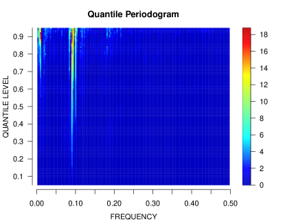
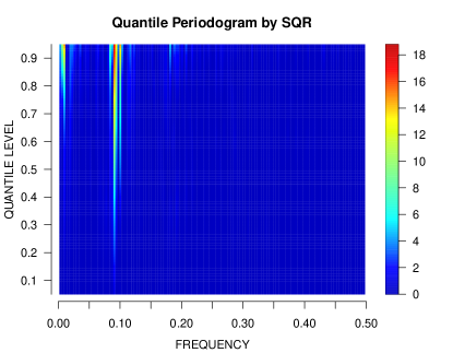
Figure 2: Time series of yearly sunspot numbers from year 1700 to 2007 $(n=308)$ and its conventional periodogram.

Figure 3: Quantile periodogram of yearly sunspot numbers constructed by trigonometric quantile regression using QR (left) and SQR with AIC (right).

Figure 4: Quantile periodogram, constructed by SQR with AIC, of yearly sunspot numbers at 11 year and 103 year frequencies. Open circles depict the result from QR.

Instead of QR, the trigonometric quantile regression can be performed by SQR. The resulting quantile periodogram is shown in the right panel of Figure 4. To construct this quantile periodogram, a single smoothing parameter is employed in the trigonometric SQR problems for all frequencies. It is chosen by minimizing the average AIC across the frequencies. Needless to say, one may also choose to employ different smoothing parameters for different frequencies to achieve greater flexibility but with higher computational burden and statistical variability.

Compared to the QR-based quantile periodogram, the SQR-based quantile periodogram appears smoother across quantiles, not only near the peaks but also in the background. The difference between these periodograms can be further appreciated by inspecting the cross-section plot in Figure 4, where the quantiles periodograms are shown as functions of the quantile level at two peak frequencies corresponding to the 11 year and 103 year cycles. The effect of smoothing is most notable in the lower curve for quantile levels higher than 0.75.

Our third example is a simulated data set of time series based on a so-called quantile autoregressive (QAR) process which satisfies

$$y_{t}=a_{0}(U_{t})+a_{1}(U_{t})\,y_{t-1}.$$ (15)

In this model, $\{U_{t}\}$ is a sequence of i.i.d. $U(0,1)$ random variables, $a_{0}(u)$ takes the form of the quantile function of $N(0,0.4^{2})$, $a_{1}(u)$ is a piecewise-linear function $0.85+0.1u+0.25(u-0.5){\cal I}(u>0.5)$. This QAR model is a slight modification of the example in Koenker (2005, p. 262) where $a_{0}(u)$ is the quantile function of $N(0,1)$ and $a_{1}(u)$ is a linear function $0.85+0.25u$.

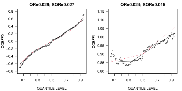
Figure 5: A simulated time series according to the QAR model (15) ($n=200$).

Figure 6: SQR estimates of $a_{0}(\cdot)$ (left) and $a_{1}(\cdot)$ (right) in (15) from the time series shown in Figure 6, where the smoothing parameter is chosen by BIC. Open circles depict the QR estimates. Dashed lines depict the true values. Absolute errors are 0.027 and 0.015 for SQR, The corresponding errors for QR are 0.026 and 0.024.

Figure 6 shows a series simulated from this QAR model ($n=200)$. Figure 6 shows the SQR estimates of the functional coefficients obtained from this series on the grid of quantile levels $\{0.05,0.06,\dots,0.96\}$, with the smoothing parameter, spar = 1.062, selected by BIC. To measure the accuracy of these estimates, we employ the absolute error which is defined as the average of absolute residuals across the quantile levels. For the SQR estimates in Figure 6, the absolute errors are 0.027 and 0.015, respectively, The corresponding errors of the QR estimates are 0.026 and 0.024. When AIC is used instead of BIC for SQR (not shown), the smoothing parameter reduces to spar = 0.835, and the absolute errors become 0.025 and 0.020. The corresponding results from SIC (not shown) yield absolute errors 0.026 and 0.019 with spar = 0.864. Clearly, a larger smoothing parameter benefits the estimate for the piecewise-linear function $a_{1}(\cdot)$, which is consistent with the underlying assumption of SQR, but may degrade the result for the nonlinear function $a_{0}(\cdot)$, which can only be approximated by piecewise-linear functions.

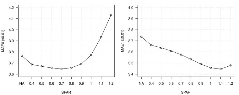
Figure 7: Mean absolute error (MAE) for estimating the functional coefficient $a_{0}(\cdot)$ (left) and $a_{1}(\cdot)$ (right) in the QAR model (15) by SQR with different values of the smoothing parameter spar. NA stands for the ordinary QR. Results are based on 1000 Monte Carlo runs with $n=200$.

This finding is confirmed by a more comprehensive analysis of the estimation accuracy based on 1000 Monte Carlo runs. The result of this analysis is shown in Figure 7, where the mean absolute error (MAE) is plotted against the smoothing parameter spar for estimating $a_{0}(\cdot)$ and $a_{1}(\cdot)$, respectively. As can be seen, the SQR estimates outperform the QR estimates for a range of smoothing parameter values, especially for estimating $a_{1}(\cdot)$. The MAE increases when the smoothing parameter is too large, especially for estimating $a_{0}(\cdot)$. The best spar for estimating $a_{0}(\cdot)$ is around 0.7 and the best spar for estimating $a_{1}(\cdot)$ is around 1.1. The total MAE for estimating both functions (not shown) is minimized when spar equals 0.9. The results in Table 1 further demonstrate that the data-driven criteria work as expected in selecting a suitable smoothing parameter. The heavier penalty in BIC benefits the estimation of $a_{1}(\cdot)$, whereas the lighter penalty in AIC benefits the estimation of $a_{0}(\cdot)$.

Table 1: Mean Absolute Error of QR and SQR Estimates for the QAR Model (15)

	Estimation of $a_{0}(\cdot)$				Estimation of $a_{1}(\cdot)$
$n$	QR	SQR-AIC	SQR-SIC	SQR-BIC	QR	SQR-AIC	SQR-SIC	SQR-BIC
200	0.0377	0.0367	0.0369	0.0378	0.0374	0.0353	0.0351	0.0349
500	0.0221	0.0219	0.0221	0.0226	0.0208	0.0195	0.0194	0.0193

Results are based on 1000 Monte Carlo run.

Our final example is the US infant birth weight data from the National Bureau of Economic Research (NBER) for year 2022. This example follows the method of Koenker (2005, p. 20) by extracting records for black or white mothers between ages 18 and 45. The study in Koenker (2005) is based on a data set for year 1997 and included 16 explanatory variables. We simplify the study in this example by considering only 8 explanatory variables for the birth weight (in grams): infant’s sex (0 for Girl, 1 for Boy), mother’s race (0 for White, 1 for Black), age (18–45), and marital status (0 for Unmarried, 1 for Married), and prenatal medical care named Precare (0 if the first visit in the first trimester of the pregnancy, 1 if no prenatal visit, 2 if the first visit in the second trimester, 3 if the first visit in the last trimester). For simplicity, mother’s education level, smoking status, and weight gain during pregnancy are not used in the model. As in Koenker (2005), we use a quadratic function to represent the effect of age.

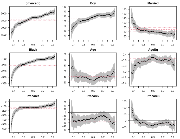
(a)

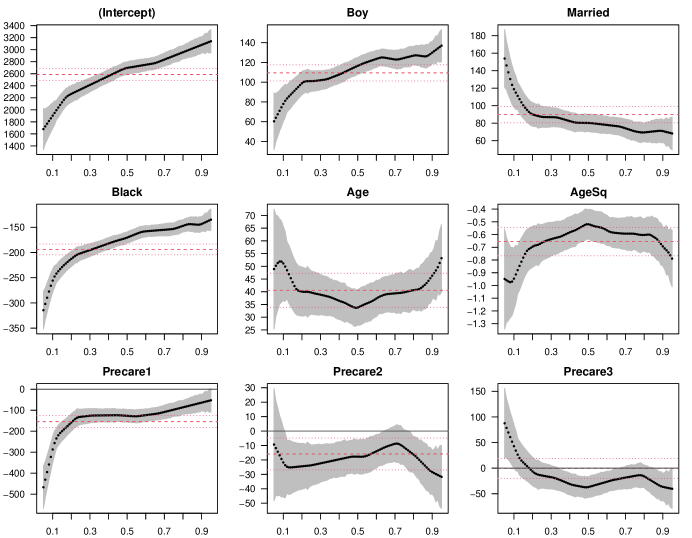
(b)

Figure 8: Quantile regression for birth weight. (a) QR estimates. (b) SQR estimates. Shaded gray area depicts a 90% pointwise confidence band.

Figure 8 depict the estimated functional coefficients by QR and SQR on the quantile grid $\{0.05,0.06,\dots,0.95\}$. These estimates are obtained from a random sample of $n=50000$ records. The 90% pointwise confidence bands (shaded grey areas) for both types of estimates are constructed using the estimated standard errors of the QR estimates under the iid assumption (se=‘iid’ in summary.rq). As in Koenker (2005, p. 21), the dashed and dotted horizontal lines depict the ordinary least-squares estimate of the mean effect and a 90% confidence interval of the estimate. The QR estimates in Figure 8(a) are very similar to those in Koenker (2005, p. 21). The SQR estimates in Figure 8(b) present the quantile-dependent effect of the explanary variables with better-defined and less-noisy patterns.

5 Gradient Algorithms

The LP method provides the exact solution to the SQR problem. However, the artificially inflated number of decision variables can be a challenge to the computer memory when $n+p$ is large. Indeed, the total number of decision variables in the primal-dual pair (11) and (12) equals $2(n+p)L+pK$, which is far greater than the $pK$ variables in the original regression coefficients. This challenge calls for alternative algorithms that consume less memory but still provide reasonably good solutions that may not be exact. Gradient algorithms, which directly optimize the objective function in (2) with respect to ${\boldsymbol{\theta}}$ in $\mathbb{R}^{pK}$, are obvious candidates.

Despite the existence of counterexamples (Asl and Overton 2020), gradient algorithms have been successfully used in practice to solve optimization problems with non-smooth objective functions (e.g., not everywhere differentiable or continuously differentiable). This is evidenced, for example, by the effectiveness of such algorithms for training neural network models involving non-smooth activation functions (Goodfellow et al. 2016; Ruder 2016). We consider three such algorithms for the SQR problem in (2), where the objective function is convex, continuous, and piecewise linear, but not everywhere differentiable.

The first algorithm is the well-known Broyden–Fletcher–Goldfarb–Shanno (BFGS) algorithm (Nocedal and Wright 2006). To supply this algorithm with a gradient function, we set the derivatives of $\rho_{\tau}(y)$ and $|y|$ to zero when $y=0$. This operation should not have a significant effect on the computed optimization solution when the overall gradient is determined jointly by many contributors, most of which having properly defined derivatives, as is likely the case for the SQR problem. The BFGS algorithm has been found effective for non-smooth problems in practice, but a general theory of convergence remains lacking. A mathematical analysis of its behavior for certain non-smooth functions including $|y|$ can be found in Lewis and Overton (2013).

The BFGS algorithm is a quasi-Newton method that uses an approximate Hessian matrix to capture the local curvature of the objective function together with a line search to find the optimal step size for each iteration. The optim function in the R package ‘stats’ (R Core Team 2024) has an option for the BFGS algorithm. This implementation employs a backtracking line search strategy and works remarkably well in our trigonometric SQR experiement. Another R implementation, bfgs (https://rdrr.io/rforge/rHanso/man/bfgs.html), takes a more aggressive bisection approach in line search, guided additionally by the so-called curvature condition (Nocedal and Wright 2006). Unfortunately, in our trigonometric SQR experiment, this implementation tends to terminate prematurely due to failures in line search.

The Hessian matrix update and the line search in BFGS are computationally expensive. For more economical alternatives, we turn to a basic gradient algorithm without the help of Hessian matrix and line search. Due to their computational simplicity, such algorithms have become increasingly popular for training neural network models (Goodfellow et al. 2016; Ruder 2016). A successful example is known as ADAM (Kingma and Ba 2015). In this algorithm, the usual gradient in a gradient descent iteration is replaced by an exponentially weighted average of all past gradients and normalized by the square root of an exponentially weighted average of squared gradients. The ADAM algorithm may oscillate around the minimizer indefinitely because the step size does not go to zero with the iteration. Therefore, it needs to be terminated after a predefined number of iterations.

Table 2: Limited Line Search in the GRAD Algorithm

Limited line search, performed periodically in GRAD after a warm-up phase.

The criterion for accepting a trial step size and the discount factor $b:=0.2$ are the same as in optim for BFGS.

(i) (ii) $s_{0}:=$ default step size, (iii) (iv) $s_{0}:=$ current step size; $\kappa_{0}:=$ number of trials.

$s\leftarrow\min\{1,s_{0}\times b^{-\lfloor\kappa_{0}/2\rfloor}\}$ (initialize trial step size); $\kappa\leftarrow 0$ (initialize trial count)

While $s$ not accepted and $\kappa<\kappa_{0}$ Do

$s\leftarrow s\times b$; $\kappa\leftarrow\kappa+1$

End While

Return (i) (iv) $s$ if accepted $s_{0}$ otherwise, (ii) (iii) $s$ if accepted $s_{0}\times b$ otherwise

The third algorithm, which we call GRAD, is an enhanced version of ADAM. In this algorithm, we modify ADAM by usng a limited line search to adjust the step size during iteration rather than holding the step size constant. The line search, shown in Table 2, follows the same backtracking strategy as in optim. However, it is performed not in every iteration but with a much lower frequency and only after a warm-up period; it is also performed with a small number of trials including both increase and decrease in step size. Furthermore. there are four options with difference choices for the starting step size and the returning step size when none of the trial step sizes are acceptable. Options (i) and (ii) start with the default step size used in the warm-up period, whereas options (iii) and (iv) start with the current step size. When the line search fails to produce an acceptable step size, options (i) and (iv) fall back to the default step size, whereas options (ii) and (iii) fall back to the discounted current step size. Note that only option (iii) offers gradually decreased step sizes when increases are unacceptable as suggested by the convergence theory of subgradient methods for nonsmooth problems (Polyak 1987). None of these options guarantees a monotone reduction in the objective function. Option (i) deviates the least from ADAM, as the step size remains at the default value except when a different trial step size becomes acceptable. Option (iv) can produce the same result as option (i) when a step size different from the default value is never found acceptable.

6 Experimentation with Gradient Algorithms

In this section, we conduct two experiments to evaluate the accuracy of the gradient algorithms discussed in the previous section as approximations to the LP solution.

The first experiment uses the Engel food expenditure data discussed earlier. Table 3 contains the total mean absolute errors of the gradient algorithms for approximating the two functional coefficients obtained by LP on the quantile grid $\{0.02,0.03,\dots,0.98\}$. The best performance is achieved by BFGS, which approximates the LP solution closely with 300 iterations (further iteration makes no significant gains). ADAM and GRAD are unable to attain such accuracy despite a large number of additional iterations. GRAD is an improvement over ADAM in reducing the approximation error. Trading memory requirement with computer time is a typical property of gradient algorithms when they work. This is the case for BFGS. An informal test shows that BFGS takes 50 seconds to complete the 300 iterations versus 12 seconds by LP.

Table 3: Approximation Error for Engel’s Food Expenditure Data

	Number of Iterations
Algorithm	0	50	100	150	200	300	400	500	1000
BFGS	6.9064	6.7616	6.6951	1.0965	0.2112	0.1316
ADAM	6.9064	6.7194	6.6910	6.6903	6.6904	6.6904	6.6904	6.6904	6.6904
GRAD	6.9064	6.7194	6.6835	6.6771	6.6774	6.6027	6.6034	6.5307	6.4270

QR is used as initial value in iteration 0. For ADAM and GRAD, warm-up phase = 70, frequency of step size update = 20, initial step size $s_{0}=0.4$, and discount factor $b=0.2$. GRAD uses option (i) for line search with $\kappa_{0}=5$.

The second experiment employs a simulated time series of length $n=512$ Motivated by the quantile periodogram (Li 2012), we compute the regression coefficients $\hat{\beta}_{1}(\tau,\omega),\hat{\beta}_{2}(\tau,\omega)$, and $\hat{\beta}_{3}(\tau,\omega)$ on the quantile grid $\tau\in\{0.10,0.11,\dots,0.90\}$ using the trigonometric regressor $\mathbf{x}_{t}(\omega):=[1,\cos(\omega t),\sin(\omega t)]^{T}$ at 255 Fourier frequencies $\omega\in\{2\pi v/n:v=1,\dots,\lfloor(n-1)/2\rfloor\}$. The coefficients $\hat{\beta}_{2}(\tau,\omega)$ and $\hat{\beta}_{3}(\tau,\omega)$, which define the quantile periodogram, are compared with the corresponding LP solutions. The average sum of squared errors across the quantiles and frequencies is used to measure the accuracy of the gradient algorithm.

The time series $\{y_{t}\}$ is generated by a nonlinear mixture model in Li (2020). For brevity, the exact form of this model is omitted here because it is not important for our discussion. It suffices to say that the 255 LP solutions have a variety of patterns based on which we evaluate the approximations produced by the gradient algorithms. One of the solutions is shown in Figure 9 together with the approximations produced by BFGS and ADAM and the corresponding QR solution. Both BFGS and ADAM are terminated after 100 iterations. As can be seen, the estimates from BFGS and ADAM appear remarkably similar to the estimates from LP.

Figure 9: Coefficients of trigonometric SQR at frequency $\omega=2\pi\times 102/512$ computed by LP (solid line), BFGS (dashed line), and ADAM (dotted line). Open circles depict the QR solution.

Figure 10 shows the the boxplot of approximation errors of BFGS and ADAM for all 255 frequencies against the number of iterations. This result confirms that both BFGS and ADAM, with sufficiently large number of iterations, provide reasonably good approximations to the LP solution. The BFGS algorithm is able to offer a higher accuracy of approximation than ADAM after an initial warm-up period. The ADAM algorithm has a more successful start in early stages of the iteration, but stops improving beyond a certain number of iterations.

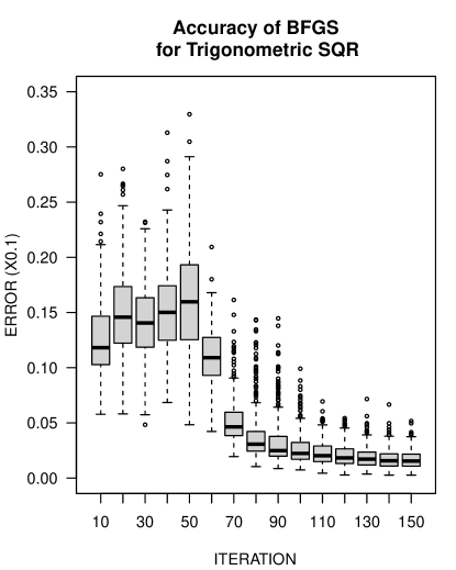
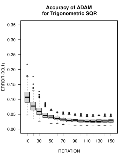
Figure 10: Boxplot of approximation errors of trigonometric SQR at 255 frequencies versus the number of iterations computed by BFGS (left) and ADAM (right).

Figure 11 compares GRAD with ADAM and BFGS based on the average approximation error across all 255 frequencies. Line search in GRAD is performed once every 10 iterations with 5 trial step sizes after 70 warm-up iterations. Thanks to these modifications, GRAD is able to outperform ADAM in terms of the approximation error and the objective function after the warm-up iterations. Among the four options in GRAD, option (iii) is most effective in reducing the objective function, whereas option (i) is least effective because it does not shrink the step size when the limited line search fails. In terms of reducing the approximation error, option (ii) turns out to be most effective.

Figure 11: Average approximation error (left) and average objective function (right) of trigonometric SQR across 255 frequencies versus the number of iterations computed by BFGS, ADAM, and GRAD with 4 options.

It is interesting to observe that after 150 iterations the average approximation error of GRAD remains much larger than that of BFGS, although the average objective function of GRAD becomes near that of BFGS. Such discrepancies are often observed in problems where the objective function has a shallow minimum in some variables. With BFGS, possible differences in curvature among variables are equalized by the Hessian matrix. This enables BFGS to move quickly toward the solution with the same step size for all variables. Being a first-order algorithm, neither GRAD nor ADAM possesses this capability. Slow improvement (if any) is expected for these algorithms due to the requirement of small step sizes.

7 Concluding Remarks

In summary, we consider the problem of fitting linear models by quantile regression at multiple quantile levels where the coefficients of regressors are represented by spline functions of the quantile level and penalized to ensure smoothness across quantiles. Using the $L_{1}$-norm of second derivatives as the penalty term, the resulting spline quantile regression (SQR) problem can be reformulated and solved as a linear program (LP) by an interior-point algorithm. The SQR solution complements the ordinary quantile regression (QR) solution obtained independently for each quantile level. Our experiments show that an improved estimate over QR can be obtained by SQR when the underlying functional coefficients are suitably smooth.

We also consider three gradient algorithms, BFGS, ADAM, and GRAD, to provide approximations to the LP solution with less computer memory, Our experiments show that it is possible for these gradient algorithms, especially BFGS, to produce reasonably good approximations to the LP solution, but a large number of iterations may be required, especially for ADAM and GRAD. The variable step size in GRAD is more effective than the fixed step size in ADAM. How to improve ADAM and GRAD to achieve a similar performance to BFGS without a significant increase of computational burden remains an interesting problem for future research.

References

Andriyana, Y., Gijbels, I., and Verhasselt, A. (2014). P-splines quantile regression estimation in varying coefficient models. Test, 23, 153–194.

Asl, A., and Overton, M. (2020). Analysis of the gradient method with an Armijo–Wolfe line search on a class of non-smooth convex functions. Optimization Methods and Software, 35, 223–242.

Belloni, A., Chernozhukov, V., Chetverikov, D., and Fernández-Val, I. (2019). Conditional quantile processes based on series or many regressors. Journal of Econometrics, 213, 4–29.

Berkelaar, M. (2022) Package ‘lpSolve’. https://cran.r-project.org/web/packages/lpSolve/lpSolve.pdf.

Bondell, H., Reich, B. and Wang, H. (2010). Noncrossing quantile regression curve estimation. Biometrika, 97, 825–838.

Goodfellow, I., Bengio, Y., and Courville, A. (2016). Deep Learning. Cambridge, MA: MIT Press.

Hao, M., Lin, Y., Shen, G., and Su, W. (2023). Nonparametric inference on smoothed quantile regression process. Computational Statistics and Data Analysis, 179, 107645.

He, X. (1997). Quantile curves without crossing. American Statistician, 51, 186–192.

He, X., Pan, X., Tan, K., and Zhou, W. (2023). Smoothed quantile regression with large-scale inference. Journal of Econometrics, 232, 367–388.

Kingma, D., and Ba, J. (2015). Adam: a method for stochastic optimization. International Conference on Learning Representations, arXiv:1412.6980.

Koenker, R. (2005). Quantile Regression. Cambridge University Press, Cambridge.

Koenker, R., and Bassett, G. (1978). Regression quantiles. Econometrica, 46, 33–50.

Koenker, R., and Ng, P. (2005). A Frisch-Newton algorithm for sparse quantile regression. Acta Mathematicae Applicatae Sinica, 21, 225–236.

Koenker, R., Ng, P., and Portnoy, S. (1994). Quantile smoothing splines. Biometrika, 81, 673–680.

Lewis, A., and Overton, M. (2013). Non-smooth optimization via quasi-Newton methods, Mathematical Programming, 141, 135–163.

Li, T.-H. (2012). Quantile periodograms. Journal of the American Statistical Association, 107, 765–776.

Li, T.-H. (2014). Time Series with Mixed Spectra. Boca Raton, FL: CRC Press.

Li, T.-H. (2020). From zero crossings to quantile-frequency analysis of time series with an application to nondestructive evaluation. Applied Stochastic Models for Business and Industry, 36, 1111–1130.

Nocedal, J., and Wright, S. (2006). Numerical Optimization, 2nd edn. New York: Springer.

Oh, H.-S., Lee, T., and Nychka, D. (2011). Fast nonparametric quantile regression with arbitrary smoothing methods. Journal of Computational and Graphical Statistics, 20, 510–526.

Portnoy, S., and Koenker, R. (1997). The Gaussian hare and the Laplacian tortoise: computability of squared-error versus absolute-error estimators. Statistical Science, 12, 279–300.

Polyak, B. (1987). Introduction to Optimization, Chapter. 5. New York: Optimization Software, Inc.

R Core Team (2024). R: A language and environment for statistical computing. R Foundation for Statistical Computing, Vienna, Austria. https://www.R-project.org/.

Ruder, S. (2016). An overview of gradient descent optimization algorithms. arXiv:1609.04747.

Wahba, G. (1975). Smoothing noisy data with spline functions. Numerische Mathematik, 24, 383–393.

Wu, Y., and Liu, Y. (2009). Stepwise multiple quantile regression estimation using non-crossing constraints. Statistics and Its Interface, 2, 299–310.

Appendix: R Functions

The following functions are implemented in the R package ‘qfa’ (version $\geq$ 4.0) available at https://cran.r-project.org and https://github.com/thl2019/QFA.

• sqr: a function that computes the SQR solution on a grid of quantile levels by the interior-point algorithm of Koenker et al.  (1994) with or without user-supplied smoothing parameter spar.

• sqdft: a function that computes the quantile discrete Fourier transform (QDFT) of time series data based on trigonometric SQR solutions on a grid of quantile levels with or without user-supplied smoothing parameter spar.

• qdft2qper: a function that converts the QDFT produced by sqdft into a quantile periodogram (QPER).

• qfa.plot: a function that produces a quantile-frequency image plot for a quantile spectrum.

• tsqr.fit: a low-level function that computes the trigonometric SQR solution on a grid of quamtile levels for a given frequency with a given smoothing parameter spar.

• sqr.fit.optim: a function that computes the SQR solution on a grid of quantile levels with a given smoothing parameter spar by BFGS, ADAM, or GRAD algorithm.