St Anne’s College Doctor of Philosophy Hilary 2023

Symmetry and Generalisation in Machine Learning

In memory of my dad, Captain Khalid El-Esedy, who would have enjoyed this being submitted at the end of Ramadan. Eid Mubarak, Baba.

And in gratitude to my mum, Linda. Thank you, Mam, for your unconditional(!) love and support.

Abstract

This work is about understanding the impact of invariance and equivariance on generalisation in supervised learning. We use the perspective afforded by an averaging operator to show that for any predictor that is not equivariant, there is an equivariant predictor with strictly lower test risk on all regression problems where the equivariance is correctly specified. This constitutes a rigorous proof that symmetry, in the form of invariance or equivariance, is a useful inductive bias.

We apply these ideas to equivariance and invariance in random design least squares and kernel ridge regression respectively. This allows us to specify the reduction in expected test risk in more concrete settings and express it in terms of properties of the group, the model and the data.

Along the way, we give examples and additional results to demonstrate the utility of the averaging operator approach in analysing equivariant predictors. In addition, we adopt an alternative perspective and formalise the common intuition that learning with invariant models reduces to a problem in terms of orbit representatives. The formalism extends naturally to a similar intuition for equivariant models. We conclude by connecting the two perspectives and giving some ideas for future work.

Chapter 1 Introduction

1.1 Motivation

We will study how invariance and equivariance affect generalisation in supervised learning. Let $\mathcal{G}$ be a group acting on sets $\mathcal{X}$ and $\mathcal{Y}$, then $f:\mathcal{X}\to\mathcal{Y}$ is invariant if $f(gx)=f(x)$ and equivariant if $f(gx)=gf(x)$, each holding for all $g\in\mathcal{G}$ and $x\in\mathcal{X}$. Invariance is the special case of equivariance where the action of $\mathcal{G}$ on $\mathcal{Y}$ is trivial. In this work, the word symmetry specifically refers to some form of invariance or equivariance.

Supervised learning is the science of extrapolation from labelled data. The basic task is as follows: given a sequence of input-output pairs $(x_{1},y_{1}),\dots,(x_{n},y_{n})$ generated by some unknown, possibly stochastic procedure, predict unseen values $(x,y)$ generated by the same procedure. Fundamentally, it is a problem of inductive inference.

More formally, let $X$ and $Y$ be random elements of $\mathcal{X}$ and $\mathcal{Y}$ respectively whose distributions are unknown. We call the sequence $(x_{1},y_{1}),\dots,(x_{n},y_{n})$ the observations and assume that they are, respectively, instances of the random variables $(X_{1},Y_{1}),\dots,(X_{n},Y_{n})$. The tuple $((X_{1},Y_{1}),\dots,(X_{n},Y_{n}))$ is called the training sample and individual elements of the training sample are training examples or just examples. We assume the training examples are distributed independently and identically to $(X,Y)$. The word data may refer to either fixed observations or the training sample depending on the context.

We formulate supervised learning as the problem of finding, given the observations, a minimiser over $f:\mathcal{X}\to\mathcal{Y}$ of

$$R[f]=\operatorname{\mathbb{E}}[\ell(f(X),Y)]$$

where $\ell:\mathcal{Y}\times\mathcal{Y}\to\mathbb{R}_{+}$ is the loss function which measures the quality of predictions. We will refer to $R$ as the risk function and to $R[f]$ as the risk of $f$; when the distinction isn’t needed we may refer to each of these as the risk. We call the candidate functions $f$ predictors or models. A learning algorithm is a map from training samples to predictors.

Without access to the distribution of $(X,Y)$ it is not possible to minimise the risk directly and, in any case, finding a minimiser of $R$ could be computational infeasible. In practice, an approximate solution is acceptable. In the same vein, theoretical study is often specialised to certain relationships between $X$ and $Y$ or the minimisation constrained to certain classes of predictors.

From a mathematical perspective, the problem of finding a predictor with small risk is critically underdetermined. Judicious choice of a predictor requires extrapolating from the finite number of observations to the general relationship between $X$ and $Y$. The term inductive bias refers loosely to a mode of extrapolation. For instance, linear predictors share an inductive bias because they extrapolate from the training sample in a conceptually similar fashion.

Symmetry is also a form of inductive bias. Along an orbit of $\mathcal{G}$, invariant models are constant while the values of equivariant models are related by the group action. Symmetry has emerged as a popular method of incorporating domain knowledge into models [34, 94, 35, 186, 57] and these models have applications in many areas. For instance, where symmetry is known to be a fundamental property of the system such as quantum chemistry [128], or where arbitrary experimenter choices or data representation give undue privilege to a specific coordinate system such as medical imaging or protein folding [188, 84]. The purpose of this thesis is to understand, insofar as it improves generalisation, whether symmetry is a good idea.

We will mostly consider the relative performance of predictors or learning algorithms and the risk provides a comparator. In particular, the statement $f$ generalises better than $f^{\prime}$ means that $R[f]\leq R[f^{\prime}]$ and generalising strictly better means a strict inequality in the same direction. We make the same comparison for learning algorithms, for which we define the risk to be the risk of the returned predictor viewed as a function of the training sample. In this case the risk is stochastic and the comparison will be in expectation. The risk of a predictor or learning algorithm, the extent to which it generalises, is the only measure of quality we consider. Although important, we do not consider other aspects such as interpretability or computational efficiency.

The theoretical study of generalisation can be considered as a narrow form of mathematical epistemology, in that it offers a quantitative formulation and analysis of the problem of induction. More practically, it has the potential to offer performance guarantees that improve the reliability of machine intelligence. In addition, theoretical analyses can provide conceptual schemes and intuitions that lead to new methods.

Closely related to generalisation is learning. A learning algorithm with range $\mathcal{F}$ is said to learn the class of functions $\mathcal{F}$ if $\exists m:(0,1)^{2}\to\mathbb{N}$ such that $\forall\epsilon,\delta\in(0,1)$ if $n\geq m(\epsilon,\delta)$ then for all distributions of $(X,Y)$, with probability at least $1-\delta$ over the training sample, the output $\hat{f}$ of the learning algorithm satisfies

$$R[\hat{f}]\leq\inf_{f\in\mathcal{F}}R[f]+\epsilon.$$

The pointwise minimum over all $m$ that satisfy the above is called the sample complexity of the learning algorithm.

The above model of learning is based on PAC learning, which was originally proposed by [170]. The variation we give is due to [76] and is known as agnostic PAC learning, because it is agnostic as to the relationship between $X$ and $Y$ [88]. See [155, 118] for further information and bibliographic remarks.

If the sample complexity of learning is established then one has non-asymptotic control of the risk of the learning algorithm. In the case of binary classification, the sample complexity of learning is governed by a combinatorial measure of complexity of $\mathcal{F}$ called the VC dimension, originally from [173]. The same idea holds for learning in other settings such as regression, just with different complexity measures, for instance the Rademacher complexity [92] or covering numbers [41]. See [11] for more.

In the case of symmetry, it seems natural to try to derive sample complexity upper bounds that reduce when $\mathcal{F}$ has the right symmetry. All prior works on the generalisation of invariant and equivariant models take some form of this approach (see Section 2.1 for a discussion) and we also give some results of this flavour in Propositions 3.3 and 6.2. However, the main goal of this thesis is to provide theory that aides the practitioner in deciding whether to incorporate symmetry (either engineered or learned) into their model. For this purpose the aforementioned results are suggestive, but insufficient.

We would like to understand the generalisation gap

$$\Delta(f,f^{\prime})=R[f]-R[f^{\prime}]$$

between predictors $f$ and $f^{\prime}$. Specifically, we are interested in the case where $f^{\prime}$ is equivariant and $f$ is not. If $\Delta(f,f^{\prime})>0$ then $f^{\prime}$ is preferable to $f$. When $f$ and $f^{\prime}$ are the outputs of learning algorithms the generalisation gap is a function of the training sample so is stochastic. In this setting, the complexity based results we mention above provide tail estimates for $R[f]$ and $R[f^{\prime}]$. However, unless these estimates turn out to be exact it is difficult even to tell the sign of $\operatorname{\mathbb{E}}[\Delta(f,f^{\prime})]$. Ultimately, the techniques of statistical learning theory are too general so we must take a different approach. We give an outline in the next section.

1.2 Overview

The technical setting and assumptions are described in Section 1.4.1. Below we give an informal overview of our main results without reference to these conditions. Throughout the work there are many examples and additional results to illustrate the utility of the approach. We make use of some standard facts which we give in Appendix A. We review related literature in Chapter 2.

Chapter 3 contains some general observations. Let $\mathcal{G}$ be a group and let $f:\mathcal{X}\to\mathcal{Y}$ be a function between two sets on which $\mathcal{G}$ acts. Define the operator

$$\mathcal{Q}f(x)=\int_{\mathcal{G}}g^{-1}f(gx)\mathop{}\!\mathrm{d}g$$

which takes any function and makes it equivariant. By exploring the properties of $\mathcal{Q}$, we establish in Lemma 3.1 that any function can be written as

$$f=\bar{f}+f^{\scaleobj{0.75}{\perp}}$$

where $\bar{f}$ is equivariant, $\mathcal{Q}f^{\scaleobj{0.75}{\perp}}=0$ and, crucially, the two terms are $L_{2}$-orthogonal as functions.

This turns out to be a useful observation. In particular, it means that on any regression task with squared-error loss and an equivariant target the generalisation gap $\Delta(f,\bar{f})$ is exactly the squared $L_{2}$-norm of $f^{\scaleobj{0.75}{\perp}}$. If $f$ is not equivariant then this is strictly positive. In other words, for any predictor $f$ that is not equivariant there is an equivariant predictor $f^{\prime}$ with strictly lower risk on all regression problems with squared-error loss and an equivariant target. Another view on this is that it gives a lower bound for not using an equivariant predictor. All of this applies equally to invariance.

These insights are applied in Chapter 4, where the main result quantifies the expected generalisation benefit of equivariance in a linear model. Theorem 4.4 concerns the generalisation gap $\Delta(f,f^{\prime})$ in the case that $f:\mathbb{R}^{d}\to\mathbb{R}^{k}$ is the minimum-norm least squares predictor and $f^{\prime}=\mathcal{Q}f$ is its equivariant version.

Let $\mathcal{G}$ act via orthogonal representations $\phi$ and $\psi$ on inputs $X\sim\operatorname{\mathcal{N}}(0,I_{d})$ and outputs $Y=h(X)+\xi\in\mathbb{R}^{k}$ respectively, where $h:\mathbb{R}^{d}\to\mathbb{R}^{k}$ is an equivariant linear map, $\operatorname{\mathbb{E}}[\xi]=0$ and $\operatorname{\mathbb{E}}[\xi^{2}]=\sigma^{2}<\infty$. Let

$$\lparen\chi_{\psi}|{}\chi_{\phi}\rparen=\int_{\mathcal{G}}\operatorname{Tr}(\psi(g))\operatorname{Tr}(\phi(g))\mathop{}\!\mathrm{d}g$$

denote the scalar product of the characters of the representations (which are real). We show in Theorem 4.4 that the generalisation benefit of enforcing equivariance in a linear model is given by

$$\operatorname{\mathbb{E}}[\Delta(f,f^{\prime})]=\mathcal{E}(n,d)+\sigma^{2}r(n,d)(dk-\lparen\chi_{\psi}|{}\chi_{\phi}\rparen)$$

where

$$r(n,d)=\begin{cases}{\frac{n}{d(d-n-1)}}&n<d-1\\ (n-d-1)^{-1}&n>d+1\\ \infty&\text{otherwise}\end{cases}$$

and $\mathcal{E}(n,d)\geq 0$ is the generalisation gap of the corresponding noiseless problem, specified exactly in Theorem 4.4, which vanishes when $n\geq d$. The divergence at the interpolation threshold $n\in[d-1,d+1]$ is consistent with the literature on double descent [75].

It’s worth emphasising that if $f^{\prime}$ is any other predictor such that $\operatorname{\mathbb{E}}[R[f^{\prime}]]\leq\operatorname{\mathbb{E}}[R[\mathcal{Q}f]]$ then the above result holds as a lower bound on $\operatorname{\mathbb{E}}[\Delta(f,f^{\prime})]$. In particular, this means that the above result applies to the case where $f^{\prime}$ is generated by transforming the features before training such that the least squares estimate is automatically equivariant, provided that the resulting predictor generalises at least as well as $\mathcal{Q}f$ in expectation over the training sample.

The quantity $dk-\lparen\chi_{\psi}|{}\chi_{\phi}\rparen$ represents the significance of the group symmetry to the task. The dimension of the space of linear maps $\mathbb{R}^{d}\to\mathbb{R}^{k}$ is $dk$, while $\lparen\chi_{\psi}|{}\chi_{\phi}\rparen$ is the dimension of the space of equivariant linear maps. We will see later that the quantity $dk-\lparen\chi_{\psi}|{}\chi_{\phi}\rparen$ represents the dimension of the space of linear maps that vanish under $\mathcal{Q}$. It is through the dimension of this space that the symmetry in the task controls the generalisation gap. Although invariance is a special case of equivariance, we find it instructive to discuss it separately. In Theorem 4.1 we provide a result that is analogous to Theorem 4.4 for invariant predictors, along with a separate proof.

In Chapter 5 we adapt and extend these results to kernel methods. We define the operator

$$\mathcal{O}f(x)=\int_{\mathcal{G}}f(gx)\mathop{}\!\mathrm{d}g$$

which takes any function and makes it invariant. Since $\mathcal{O}$ is a special case of $\mathcal{Q}$, we have the decomposition $f=\bar{f}+f^{\scaleobj{0.75}{\perp}}$ with $\bar{f}$ invariant, $\mathcal{O}f^{\scaleobj{0.75}{\perp}}=0$ and the terms being $L_{2}$-orthogonal. In Theorem 5.1 we study the generalisation gap $\Delta(f,\mathcal{O}f)$ for kernel ridge regression on an invariant target. The comments made above about the use of $\mathcal{Q}f$ as a comparator apply here to $\mathcal{O}f$.

Let $X$ be invariant in distribution, so $X\overset{\text{d}}{=}gX$ for all $g\in\mathcal{G}$, and set $Y=f^{*}(X)+\xi$ with $f^{*}$ invariant and $\operatorname{\mathbb{E}}[\xi]=0$, $\operatorname{\mathbb{E}}[\xi^{2}]=\sigma^{2}<\infty$. Let $f$ be the solution to kernel ridge regression with kernel $k$ and regularisation parameter $\rho>0$ on $n$ i.i.d. training examples $((X_{i},Y_{i}):i=1,\dots,n)$ each distributed identically to and independently from $(X,Y)$. In Theorem 5.1, we find that

$$\operatorname{\mathbb{E}}[\Delta(f,\mathcal{O}f)]\geq\mathcal{E}_{k}(n,\rho)+\sigma^{2}\frac{\lVert(\operatorname{\operatorname{id}}-\mathcal{O})k\rVert_{{L_{2}(\mu\otimes\mu)}}^{2}}{(\sqrt{n}M_{k}+\rho/\sqrt{n})^{2}}$$

where for any $j:\mathcal{X}\times\mathcal{X}\to\mathbb{R}$

$$\lVert j\rVert^{2}_{L_{2}(\mu\otimes\mu)}=\int_{\mathcal{X}}j(x,y)^{2}\mathop{}\!\mathrm{d}\mu(x)\mathop{}\!\mathrm{d}\mu(y),$$

$M_{k}=\sup_{x}k(x,x)<\infty$ and $\mathcal{E}_{k}(n,\rho)\geq 0$ is the generalisation gap for the corresponding noiseless problem. By considering the linear kernel we study how this result relates to the result for invariance in Chapter 4.

Further, we show that under mild additional conditions on $\mathcal{X}$, $\mathcal{Y}$ and $\rho$, $\mathcal{E}_{k}(n,\rho)\to 0$ as $n\to\infty$ provided the kernel $k$ satisfies the identity

$$\int_{\mathcal{G}}k(gx,y)\mathop{}\!\mathrm{d}g=\int_{\mathcal{G}}k(x,gy)\mathop{}\!\mathrm{d}g$$

for all $x,y\in\mathcal{X}$. Assuming this condition holds, we derive an independent result about the structure of the RKHS $\mathcal{H}$. In particular, Theorem 5.2 says that the above condition on the kernel implies the orthogonal decomposition $\mathcal{H}=\mathcal{O}\mathcal{H}\oplus(\operatorname{\operatorname{id}}-\mathcal{O})\mathcal{H}$ where the orthogonality is now with respect to the inner product on $\mathcal{H}$.

In Chapter 6 we take a different approach, making use of the observation that an invariant function can be specified by its values on one representative from each orbit of $\mathcal{X}$ under $\mathcal{G}$. We show rigorously how learning a class of invariant predictors is equivalent to learning in a reduced problem in terms of orbit representatives and extend this framework to provide a new intuition for learning equivariant predictors. In addition, we show how to use these equivalences to derive a sample complexity bound for learning invariant/equivariant classes with empirical risk minimisation.

We conclude in Chapter 7 with a relation of the orbit averaging viewpoint on invariance in Chapter 3 to the orbit representative viewpoint in Chapter 6, applications to neural networks, connections to other works and, finally, some sugggestions for future work.

1.3 Authorship

The work in this thesis is based on [52, 51, 50]. The majority of content has been revised or generalised, sometimes substantially, and some new results are given. Chapters 3, 4 and 7.2 are based on [52], Chapter 5 is based on [51] and Chapter 6 is based on [50].

All original contributions of the thesis were discovered and proved by the author unless explicitly stated otherwise. Where possible, Zaidi’s contributions to [52] are cited explicitly. Otherwise, his contributions to [52] were through discussions, proof reading and presentation. In addition, Zaidi suggested the connection to test time augmentation described in Section 3.3.2.

A list of other work completed during this DPhil is given in Appendix B.

1.4 Preliminaries

We assume familiarity with the basic notions of group theory including the definitions of a group action and a linear representation. The reader may consult [179, 154, Chapters 1-4] for background. We run through some results that we use often in Section 1.4.3. We provide some background definitions and technical material in Section 1.4.4.

1.4.1 Setup, Assumptions and Technicalities

In this section we outline our setup and technical conditions which, unless stated otherwise, are assumed throughout. Additional definitions and assumptions are given as needed. Technical conditions are chosen so as to vary the least between results; the reader interested in more general settings is encouraged to inspect the proofs. That said, the conditions we impose are quite general.

1.4.1.1 Spaces

There will be a background probability space $(\Omega,\mathcal{S}_{\Omega},\operatorname{\mathbb{P}})$ that is assumed to be rich enough to support our analysis. The input and output spaces will be $\mathcal{X}$ and $\mathcal{Y}$ respectively, where $\mathcal{X}$ is a non-empty Polish space and $\mathcal{Y}$ is $\mathbb{R}^{k}$ with an inner product $\langle\cdot,\cdot\rangle:\mathbb{R}^{k}\times\mathbb{R}^{k}\to\mathbb{R}$, induced norm $\lVert\cdot\rVert$ and corresponding topology. Sometimes $k=1$ or this inner product is the Euclidean one, but this will be specified. All $\sigma$-algebras will be Borel. In particular this makes $(\mathcal{X},\mathcal{S}_{\mathcal{X}})$ and $(\mathcal{Y},\mathcal{S}_{\mathcal{Y}})$ standard Borel spaces, but we won’t make direct use of this level of detail. Unless stated otherwise, $X$ and $Y$ will be random elements of $\mathcal{X}$ and $\mathcal{Y}$ respectively.

1.4.1.2 Group and Action

Let $\mathcal{G}$ be a measurable, second countable, Hausdorff and compact topological group. Let the Haar measure on $\mathcal{G}$ be $\lambda$, normalised so that $\lambda(\mathcal{G})=1$. This is the unique invariant probability measure on $\mathcal{G}$. We assume that $\mathcal{G}$ has a measurable action $\phi$ on $\mathcal{X}$ and measurable representation $\psi$ on $\mathcal{Y}$. By measurable we mean that $\phi:\mathcal{G}\times\mathcal{X}\to\mathcal{X}$ is a measurable map and the same for $\psi$. We will assume that $\psi$ is unitary with respect to $\langle\cdot,\cdot\rangle$, by which we mean that $\langle\psi(g)a,\psi(g)b\rangle=\langle a,b\rangle$ $\forall a,b\in\mathbb{R}^{k}$ and $\forall g\in\mathcal{G}$. Notice that this implies $\langle\psi(g)a,b\rangle=\langle a,\psi(g^{-1})b\rangle$. If $\langle\cdot,\cdot\rangle$ is the Euclidean inner product, then this is the usual notion of an orthogonal representation (one for which the $\psi(g)$ is always an orthogonal matrix). Any inner product can be transformed to be such that $\psi$ is unitary using the Weyl trick $\langle a,b\rangle\mapsto\int_{\mathcal{G}}\langle\psi(g)a,\psi(g)b\rangle\mathop{}\!\mathrm{d}\lambda(g)$. The character of a representation $\psi$ is defined by $\chi_{\psi}(g)=\operatorname{Tr}(\psi(g))$. The inner product of characters is defined by

$$\lparen\chi_{1}|{}\chi_{2}\rparen=\int_{\mathcal{G}}\chi_{1}(g)\chi_{2}(g)\mathop{}\!\mathrm{d}\lambda(g).$$

This definition typically appears with a complex conjugate, but it’s not needed because all the representations we encounter are real. The inner product of the characters of two finite-dimensional real representations of a compact group is equal to the dimension of the space of linear maps that are equivariant with respect to these representations, e.g., see [4, Theorem 3.34].

1.4.1.3 Invariance, Equivariance and Symmetry

A function $f:\mathcal{X}\to\mathcal{Y}$ is $\mathcal{G}$-invariant if $f(\phi(g)x)=f(x)$ and is $\mathcal{G}$-equivariant if $f(\phi(g)x)=\psi(g)f(x)$, each holding for all $x\in\mathcal{X}$ and for all $g\in\mathcal{G}$. Invariance is the special case of equivariance where $\psi$ is the trivial representation, i.e., $\psi(g)$ is the identity for all $g\in\mathcal{G}$. A measure $\mu$ on $\mathcal{X}$ is $\mathcal{G}$-invariant if for all $g\in\mathcal{G}$ and any $\mu$-measurable $B\subset\mathcal{X}$ the pushforward of $\mu$ by the action $\phi$ equals $\mu$, i.e., $(\phi(g)_{*}\mu)(B)=\mu(B)$. This means that if $X\sim\mu$ then $\phi(g)X\sim\mu$ for all $g\in\mathcal{G}$. We say that $X$ is $\mathcal{G}$-invariant in distribution or just $\mathcal{G}$-invariant if $X\overset{\text{d}}{=}gX$ for all $g\in\mathcal{G}$.

We will often drop the $\mathcal{G}$- when the group is clear from the context and just say invariant/equivariant. We will often also drop $\psi$ and $\phi$, so the quantity $g^{-1}f(gx)$ should be interpreted as $\psi(g^{-1})f(\phi(g)x)$, and so on. We sometimes use the catch-all term $\mathcal{G}$-symmetric to describe an object that is invariant or equivariant.

1.4.1.4 Function Space

Throughout, $\mu$ will be a $\mathcal{G}$-invariant probability measure on $(\mathcal{X},\mathcal{S}_{\mathcal{X}})$. We consider ${L_{2}(\mathcal{X},\mathcal{Y},\mu)}$, which we define to be the Hilbert space of equivalence classes of functions $f:\mathcal{X}\to\mathcal{Y}$ such that $\lVert f\rVert_{\mu}<\infty$ where the norm is induced by the following inner product

$$\langle f,h\rangle_{\mu}=\int_{\mathcal{X}}\langle f(x),h(x)\rangle\mathop{}\!\mathrm{d}\mu(x).$$

Equality in ${L_{2}(\mathcal{X},\mathcal{Y},\mu)}$ is defined $\mu$-almost-everywhere. This space is general enough to cover pretty much any predictor used in machine learning. In the case $\mathcal{Y}=\mathbb{R}$ we consider the usual $L_{2}$-space which we write ${L_{2}(\mu)}$, where the inner product on $\mathcal{Y}$ is just multiplication.

1.4.1.5 Averaging Operator

The averaging operator $\mathcal{Q}$ will be central to much of this work. It has values

$$\mathcal{Q}f(x)=\int_{\mathcal{G}}g^{-1}f(gx)\mathop{}\!\mathrm{d}\lambda(g),$$

where $\lambda$ is the normalised Haar measure on $\mathcal{G}$ with $\lambda(\mathcal{G})=1$. The operator $\mathcal{Q}$ can be used to transform any function into an equivariant function. Due to the compactness of $\mathcal{G}$, we can change variables $g\mapsto g^{-1}$ above and view $\mathcal{Q}$ as averaging the action of $\mathcal{G}$ on ${L_{2}(\mathcal{X},\mathcal{Y},\mu)}$ defined by $f\mapsto g\circ f\circ g^{-1}$. Our developments will apply equally to the operator

$$\mathcal{O}f(x)=\int_{\mathcal{G}}f(gx)\mathop{}\!\mathrm{d}\lambda(g)$$

which is the special case of $\mathcal{Q}$ in which $\psi$ is the trivial representation. In this case the action of $\mathcal{G}$ on ${L_{2}(\mathcal{X},\mathcal{Y},\mu)}$ defined above is akin to the regular representation. The operator $\mathcal{O}$ enforces invariance, a special case of equivariance. In other works both $\mathcal{O}$ and $\mathcal{Q}$ are often referred to as Reynolds operators.

1.4.2 Additional Notation

The sets $\mathbb{R}$, $\mathbb{Z}$, $\mathbb{N}$ and $\mathbb{R}_{+}$ denote the reals, integers, naturals and non-negative reals respectively. We use $\circ$ for function composition $(f\circ h)(x)=f(h(x))$ and we write $\mathsf{e}=\exp(1)$. For functions $f,h:\mathbb{N}\to\mathbb{R}_{+}$, $f=\omega(h)$ means $\exists C>0$ $\exists m\in\mathbb{N}$ such that $\forall n>m$ $f(n)>Ch(n)$ and $f=O(h)$ means $f(n)\leq Ch(n)$ under the same quantifiers.

We write $X\sim\mu$ to mean that $X$ has distribution $\mu$. For probability spaces $(S,\mathcal{S},\mu)$ and $(T,\mathcal{T},\nu)$ the product measure is denoted by $\mu\otimes\nu$, see Theorem 1.2. For random variables $A$ and $B$ independence is written $A\perp\!\!\!\perp B$, equality in distribution is written $A\overset{\text{d}}{=}B$ and almost sure equality is written $A\overset{\text{a.s.}}{=}B$. We write i.i.d. to stand for independent and identically distributed.

We will use the Einstein summation convention, in which repeated indices are implicitly summed over. The Kronecker tensor is written as $\delta_{ij}$, which is $1$ when $i=j$ and $0$ otherwise. We write $\mathbb{G}_{n}(\mathbb{R}^{d})$ for the Grassmannian manifold of subspaces of dimension $n$ in $\mathbb{R}^{d}$.

We write $\operatorname{\operatorname{id}}$ for the identity operator and any linear operator $A$ we write its adjoint as $A^{*}$. We use $\lVert\cdot\rVert_{2}$ for the Euclidean norm of vectors, $\lVert\cdot\rVert_{1}$ for the sum of magnitudes of components and $\lVert\cdot\rVert_{\infty}$ for the component-wise max magnitude. On a function $f:\mathcal{X}\to\mathbb{R}^{d}$, $\lVert f\rVert_{\infty}=\sup_{x\in\mathcal{X}}\lVert f(x)\rVert_{\infty}$.

We write $I$ for the identity matrix, sometimes with a subscript to indicate the dimension of the space on which it acts. We write $\mathbb{R}^{m\times n}$ for the set of all real matrices with $m$ rows and $n$ columns. For any matrix $A\in\mathbb{R}^{n\times n}$ we define $\lVert A\rVert_{2}=\sup_{x\in\mathbb{R}^{n}}\frac{\lVert Ax\rVert_{2}}{\lVert x\rVert_{2}}$, which is the operator norm induced by the Euclidean norm. In general, the operator norm of any operator between normed spaces will be written with $\lVert\cdot\rVert_{\text{op}}$. For any symmetric matrix $A$, we denote by $\gamma_{\text{max}}(A)$ and $\gamma_{\text{min}}(A)$ the largest and smallest eigenvalues of $A$ respectively. For any matrix $A$ we write $A^{+}$ for the Moore-Penrose pseudo-inverse and $\lVert A\rVert_{\text{F}}=\sqrt{\operatorname{Tr}(A^{\top}A)}$ for the Frobenius norm.

Some notation for specific groups: $\mathsf{C}_{m}$ and $\mathsf{S}_{m}$ are, respectively, the cyclic and symmetric groups on $m$ elements, while $\mathsf{O}_{m}$ and $\mathsf{SO}_{m}$ are the $m$-dimensional orthogonal and special orthogonal groups respectively. The group of $m\times m$ invertible real matrices is written $\mathsf{GL}_{m}$.

1.4.3 Commonly Used Results

We will make use of the results in this section throughout the work.

The inclusion ${L_{2}(\mu)}\subset L_{1}(\mu)$

Theorem 1.1 ([174, Theorem 2]).

Let $(\mathcal{X},\mathcal{S}_{\mathcal{X}},\mu)$ be a measure space with $\mu\geq 0$. Let $A_{\infty}=\{A\in\mathcal{S}_{\mathcal{X}}:\mu(A)<\infty\}$. Then $\sup_{A\in A_{\infty}}\mu(A)<\infty$ is equivalent to $L_{p}(\mu)\subset L_{q}(\mu)$ for all $p>q$.

In our case $\mu$ is a probability measure, so ${L_{2}(\mu)}\subset L_{1}(\mu)$. We will use this fact frequently, in particular when applying Fubini’s theorem.

Fubini’s theorem

Theorem 1.2 (Fubini’s theorem [85, Theorem 1.27]).

For any $\sigma$-finite measure spaces $(S,\mathcal{S},\nu_{S})$ and $(T,\mathcal{T},\nu_{T})$ there exists a unique product measure $\nu=\nu_{S}\otimes\nu_{T}$ on $(S\times T,\mathcal{S}\otimes\mathcal{T})$ such that

$$\nu(A\times B)=\nu_{S}(A)\nu_{T}(B)\quad\forall A\in\mathcal{S},\;B\in\mathcal{T}.$$

Moreover, for any measurable $f:S\times T\to\mathbb{R}_{+}$

$$\int_{S\times T}f(s,t)\mathop{}\!\mathrm{d}\nu(s,t)=\int_{S}\mathop{}\!\mathrm{d}\nu_{S}(s)\int_{T}f(s,t)\mathop{}\!\mathrm{d}\nu_{T}(t)=\int_{T}\mathop{}\!\mathrm{d}\nu_{T}(t)\int_{S}f(s,t)\mathop{}\!\mathrm{d}\nu_{S}(s).$$

The above remains valid for any $\nu$-integrable $f:S\times T\to\mathbb{R}$.

Both $\mu$ and $\lambda$ are probability measures so are $\sigma$-finite. When the integrand can be negative we must verify integrability. In doing this, we will might apply Fubini’s theorem to a non-negative function, but most of the time we will use Theorem 1.1.

Change of variables $g\mapsto g^{-1}$

Theorem 1.3 ([58, Corollary 2.28 and Proposition 2.31]).

Let $\mathcal{G}$ be a measurable compact group with Haar measure $\lambda$, then $\mathop{}\!\mathrm{d}\lambda(g)=\mathop{}\!\mathrm{d}\lambda(g^{-1})$.

1.4.4 Background Theory

We list some background definitions and results. For more details see [143, 85].

1.4.4.1 Topology

A topological space is separable if it contains a countable dense subset.

A metric space is complete if every Cauchy sequence in the space converges to a limit in the space.

A Polish space is a separable topological space that admits a metric with respect to which it is complete.

Let $(T,\tau)$ be a topological space, then $B\subset\tau$ is a base for $\tau$ if any element of $\tau$ is the union of elements of $B$.

A topological space is second countable if its topology has a countable base.

A topological space is Hausdorff if all pairs of distinct points have disjoint open neighbourhoods.

A subset of a topological space is compact if every open cover has a finite sub-cover and it is locally compact if every point has a compact neighbourhood. Clearly, any compact set is locally compact.

A topological group is a group $\mathcal{G}$ equipped with topology such that the group operations are continuous. For instance $g\mapsto g^{-1}$ is continuous and $(g,h)\mapsto gh$ is continuous when $\mathcal{G}^{2}$ has the product topology.

1.4.4.2 Measure Theory

Let $f:A\times B\to C$ be a function. Then a $B$-section of $f$ is a function $f_{b}:A\to C$ for some $b\in B$ with $f_{b}(a)=f(a,b)$. An $A$-section is defined similarly.

Let $(S,\mathcal{S},\nu)$ be a measure space. We say $\nu$ is $\sigma$-finite if $S$ can be written as the disjoint union of a countable family of elements of $\mathcal{S}$, each of which has finite measure. All probability measures are $\sigma$-finite.

The Borel $\sigma$-algebra on a topological space is the $\sigma$-algebra generated by the topology. A Borel measure is a measure defined on a Borel $\sigma$-algebra.

A measurable group is a measurable space $(\mathcal{G},\mathcal{S}_{\mathcal{G}})$ where $\mathcal{G}$ is a topological group and $\mathcal{S}_{\mathcal{G}}$ is the Borel $\sigma$-algebra. In this case the group operations are measurable when $\mathcal{G}$ is locally compact, second countable and Hausdorff [85, p. 39].

A measure $\lambda$ on $(\mathcal{G},\mathcal{S}_{\mathcal{G}})$ is left-invariant if $\lambda(gA)=\lambda(A)$ for all $A\in\mathcal{S}_{\mathcal{G}}$ and for all $g\in\mathcal{G}$. The definition of right-invariant is the same but with $\lambda(Ag)=\lambda(A)$. The measure $\lambda$ is invariant if it is both left-invariant and right-invariant.

A Radon measure is one that is finite on any compact measurable set.

Theorem 1.4 (Haar measure [85, Theorem 2.27]).

On any locally compact, second countable and Hausdorff measurable group $\mathcal{G}$ there exists, uniquely up to normalisation, a left-invariant Radon measure $\lambda$ with $\lambda\neq 0$. If $\mathcal{G}$ is compact then $\lambda$ is also right-invariant.

In our setting $\mathcal{G}$ will be compact so we can normalise $\lambda$ to be the unique invariant probability measure.

Chapter 2 Related Literature

In this work we are concerned with predictors that are equivariant or invariant functions. In particular we are interested in a theoretical analysis of their generalisation. We discuss works in this area first in Section 2.1, then move on to an outline of various symmetric models and their applications in Section 2.2. We end this chapter with Section 2.3, in which we point to some other notions of symmetry in machine learning.

We note that group symmetry plays a role in the nearby field of statistics. We do not discuss this, but instead refer the reader to [49, 22, 21] and references therein. Finally, in writing this literature review we found results that are either related to or are special cases of the results in this thesis. We give a comparison in Section 7.3.

2.1 Symmetry and Generalisation

The first general theoretical justification for invariance of which we are aware is from [64, 3], which, roughly, states that enforcing invariance cannot increase the VC dimension of a model. Prior to that, the specific case of neural networks was addressed by John Shawe-Taylor, who calculated sample complexity bounds for neural networks whose weights can be partitioned into equivalence classes, which is directly applicable to invariant/equivariant networks [161, 159].

A heuristic argument for reduced sample complexity for invariant models is made by [120] in the case that the input space has finite cardinality. The sample complexity of linear classifiers with invariant representations trained on a simplified image task is discussed briefly by [10], the authors conjecture that a general result may be obtained using wavelet transforms. A similar argument for sample complexity reduction due to translation invariance is made by [7, 9] where it is argued that the sample complexity depends on the input space, which is, in effect, significantly smaller from the perspective of a translation invariant model. This idea is prevalent in the literature and is captured rigorously in Section 6.4.

Indeed, there are many sample complexity results that are similar in spirit to those in Section 6.4, where we consider coverings on the hypothesis class and input space that reduce for invariant/equivariant hypotheses. This result, along with the rest of Chapter 6, is relatively recent work [50]. Earlier, [165] built on the work of [192] by considering classifiers that are invariant to a finite set of transformations. Their results apply to the case where the metric on the input space is the Euclidean norm contain an implicit margin constraint on the training data. [145] prove a generalisation bound for invariant/equivariant neural networks in the case of finite groups in terms of covering numbers of the quotient space $\mathcal{X}/\mathcal{G}$. [198] use a pseudo-metric that exploits the group action to express the covering number of the hypothesis class on the training set in terms of a covering number of the hypothesis class on the orbit of the training set under the group action. The work of [156] was published concurrently with what is presented in Chapter 6 and, at least in its learning-theoretic perspective, is most closely related. Their main results include upper and lower sample complexity bounds for learning with invariant hypotheses on an invariant distribution in terms of an adaptation of the VC dimension that incorporates the group action [156, Theorem 4].

At a high level, all but three works on the generalisation of invariant/equivariant models of which we are aware construct a generic generalisation bound that can be shown to reduce under the assumption that the class of predictors satisfies a symmetry. [20] study the restricted setting of a discrete grid for the input space and subsets of the symmetric group for symmetries, and use spherical harmonics to derive a sample complexity upper bound for kernel ridge regression that reduces by a factor of the size of the group for invariant kernels. Notably, their setup is a special case of our condition Eq. 5.3.1 with a finite group and an inner product kernel [20, Eq. 8]. [109] study the effect of symmetry on the marginal likelihood and use this for model selection. [16] consider equivariant networks in the Fourier domain to derive norm based PAC Bayes generalisation bounds. [184] study lower bounds for the generalisation error of equivariant predictors when the symmetry is misspecified to varying degrees. [169] derive upper and lower sample complexity bounds for invariant kernel regression on manifolds.

However, all of the aforementioned works are worst-case, in the sense that they give sample complexity bounds that apply to an entire class of predictors simultaneously. Of course, this does not guarantee that the generalisation of any given predictor (at a fixed number of examples) would be improved if it were somehow replaced with an invariant/equivariant one. This issue was not resolved until [52], one of the works contributing to this thesis, wherein it was shown in an abstract setting that for any predictor that is not invariant/equivariant there is an invariant/equivariant predictor with strictly lower risk on all regression tasks with an invariant/equivariant target. Explicit calculations of this generalisation improvement were given for linear models [52, Theorem 7 and Theorem 13] and subsequently for kernel ridge regression in a separate work which also forms part of this thesis [51]. Concurrently, [116] analyse the asymptotic generalisation benefit of invariance in random feature models and kernel methods, providing the only other strict generalisation benefit for invariance of which we are aware. A comparison of their results to the relevant results in this thesis is given in Section 7.3.

2.2 Invariant and Equivariant Models

While there has been a recent surge in interest, symmetry and invariance have a long history in machine learning, for instance appearing in the classical work of [63]. See [190] and references therein. The vast majority of modern implementations concern multi-layer perceptrons (MLPs) and variations of convolutional neural networks (CNNs) and our focus will reflect this. However, implementation of invariance/equivariance in other models has been explored too, as we outline below.

2.2.1 The Symmetric Zoo

Invariance and equivariance have been implemented in various models in machine learning and related areas. To name a few: steerable filters for image processing [60], invariance in signal processing [81] and scattering transforms [111, 28], kernels [70, 71, 196, 136], support vector machines [149, 29, 42, 183] and feature spaces of invariant polynomials [151, 152, 72].

In addition, recent works include equivariant Gaussian processes and neural processes [80], capsule networks [104], self attention and transformers [82, 78, 61, 62], autoencoders [193, 189], normalising flows [140, 91, 148, 25] and graph networks [113, 147, 130], whose approximation capacity has been studied by [14].

Methods and results also exist that can be applied to a range of models. Of course, averaging any predictor over the group with $\mathcal{O}$ or $\mathcal{Q}$ produces invariance or equivariance respectively but is often computationally infeasible. [130] find a computationally tractable alternative by averaging over a selected subgroup. Taking a viewpoint similar to Chapter 6, [13] propose to learn invariant/equivariant models by projecting the data onto a space of orbit representatives. [176] show how functions equivariant to physical symmetries such as rigid body transformations and the Lorentz group can be expressed solely in terms of invariant scalar functions. In a similar vein, [23] show how to parameterise polynomial or smooth equivariant functions in terms of invariant ones. Finally, [7] discuss the foundations of learning representations that are both invariant and selective, meaning that the representations for two inputs are equal only if the inputs belong to the same orbit.

2.2.2 Equivariant MLPs and CNNs

The design of invariant neural networks was first considered by Shawe-Taylor and Wood, in which ideas from representation theory are applied to find weight tying schemes in MLPs that result in group invariant architectures [157, 160, 158, 191]. Similarly, [138] observe that the equivariance in a linear map $\mathbb{R}^{d}\to\mathbb{R}^{k}$ implies symmetries in the corresponding weight matrix $M\in\mathbb{R}^{k\times d}$ and use this to derive weight tying schemes for equivariant neural networks. [56] reduce layer-wise equivariance of the network to a finite dimensional linear system that the weights must satisfy and use this to engineer equivariant MLPs, their method works even for infinite Lie groups (provided they have finite dimension). [162] take a different route, regularising the directional derivatives of the learned model to encourage invariance to local transformations.

For CNNs, weight tying for equivariance to $90^{\circ}$ rotations was proposed by [45]. A weight-tying approach for arbitrary symmetry groups was developed for CNNs by [65] using kernel interpolation. [112] apply convolutional filters at a range of orientations to produce rotation equivariant networks. To achieve rotation invariance, [89] map images to polar co-ordinates before performing the convolution. In addition, an equivariant version of the subsampling/upsampling operations in CNNs was proposed by [193].

It is well known that CNNs are equivariant to (local) translations [103] and this is widely believed to be a key factor in their generalisation performance. The G-CNN was introduced by [34] who, by viewing the standard convolutional layer as the convolution operator on feature maps over the translation group, generalised the convolutional layer to be equivariant to other groups that preserve the two dimensional lattice $\mathbb{Z}^{2}$. Following this were many works borrowing ideas from harmonic analysis, representation theory and mathematical physics to generalise the basic approach of the G-CNN to various groups and input spaces [36, 37, 54, 94, 35, 186, 57, 187]. [53] gives an exposition of some of these models and the underlying mathematical concepts.

Following the introduction of the G-CNN, [95] show that any equivariant neural network layer on a homogeneous space (one for which $\forall x,y\in\mathcal{X}$ $\exists g\in\mathcal{G}$ such that $x=gy$) can be expressed in terms of a group convolution. This was elegantly generalised to non-homogeneous spaces by [129, Section 4.3]. [98] give a general parameterisation for the filters in these equivariant convolutions that holds for any compact group. Getting even more general, [22] characterise the structure of invariant/equivariant probability distributions using an extension of noise outsourcing (also known as transfer) [85, Theorem 6.10] to connect functional and probabilistic symmetries.

There are results that establish, across a variety of settings, that any continuous invariant/equivariant function can be approximated to arbitrary accuracy with an invariant/equivariant neural network [194, 137, 115]. In addition, [99] study efficient approximation of smooth functions using neural network architectures that are invariant to subgroups of the orthogonal group. While [132] compare the computational complexity of two layer ReLU networks with similar equivariant networks.

There are also works specialised to the theory of learning equivariant neural networks. [19] study the invariance, stability and sample complexity of convolutional neural networks with smooth homogeneous activation functions by embedding them in a certain reproducing kernel Hilbert space. [127] estimate the VC dimension of G-CNNs and prove the existence of two layer G-CNNs that are invariant to an infinite group, yet have infinite VC dimension. [100] analyse the implicit bias of linear G-CNNs when trained by gradient descent, while [32] study the implicit bias of linear equivariant steerable CNNs trained by gradient flow.

A sub-field has emerged for learning functions on sets. We discuss permutation symmetry in more detail below but briefly mention a few related works now. [114] study the learning of functions on sets whose elements themselves satisfy symmetries. [185] construct architectures for hierarchical symmetries, such as permutation equivariant maps of sets (that themselves are invariant to permutation of their elements) and apply it to semantic segmentation of point cloud data. A transformer for use on set valued data was developed by [101].

2.2.2.1 Permutation Equivariance

Particular attention has been paid to neural networks $f:\mathbb{R}^{n}\to\mathbb{R}^{m}$ that are equivariant to the action of the permutation group $\mathsf{S}_{n}$ on their inputs. The representation corresponding to $\pi\in\mathsf{S}_{n}$ on the inputs is the natural action $f(x_{1},\dots,x_{n})\mapsto f(x_{\pi^{-1}(1)},\dots,x_{\pi^{-1}(n)})$. The most common representations on the outputs are the trivial representation, the natural representation when $m=n$, or $\operatorname{sign}(\pi)$ where here $\operatorname{sign}$ denotes the $\operatorname{sign}$ of the permutation $\pi$, which is the parity of the product of the parities of the transpositions in its decomposition thereof. These three possibilities fall under the names of permutation invariant, permutation equivariant and fermionic networks respectively. Fermionic networks are also known as anti-symmetric networks, which is a special case of the usage of the term $\mathcal{G}$-anti-symmetric in this work. In particular, it is straightforward to see that if $f$ is a fermionic network, then one must have $\mathcal{O}f=0$ if $n>1$.

[195] propose the use of permutation invariant neural networks for tasks with inputs that are sets and show that any continuous permutation invariant function $f:[0,1]^{n}\to\mathbb{R}$ must have the form

$$f(x)=f_{1}\left(\sum_{i=1}^{n}f_{2}(x_{i})\right)$$ (2.2.1)

for some continuous functions $f_{1}$ and $f_{2}$ with $f_{2}$ independent of $f$. The importance of continuity and the dimension of any intermediate latent spaces used in the computation of $f$ (of particular relevance to neural networks) is considered by [180, 181]. In a sense, these results say that the only permutation invariant function is summation.

There has been considerable work on the theory of permutation equivariant networks. [2, 83] consider approximating and representing fermionic functions in terms of sums of determinants respectively. [73] study approximating permutation invariant and fermionic functions. While universal approximation of permutation equivariant functions was proved by [146, 153]. Finally, [122] study the ability of a generic two layer neural network to learn a certain class of permutation invariant functions.

One application of permutation invariant networks is point cloud modelling. Point cloud networks are permutation invariant neural networks that are designed to preserve the shape of point clouds [131]. Point cloud networks may also be invariant or equivariant to rigid body transformations (translation and rotation) and have applications in computer vision and robotics [68]. Their approximation properties have been studied by [48].

2.2.3 A Remark on the Representation of Invariant Functions

The work from [22] which we referred to earlier offers a probabilistic generalisation of Eq. 2.2.1 in an analogous expression for random variables. Permutations are generalised to any compact group and the sum is replaced with a maximal invariant, which is a function $M$ on $\mathcal{X}$ that takes a distinct constant value on each orbit of $\mathcal{X}$ under $\mathcal{G}$. That is, $M$ is invariant and $M(x)=M(y)$ implies $gx=y$ for some $g\in\mathcal{G}$. As it happens, using the below theorem, if there exists a function $\varphi$ such that $\mathcal{O}\varphi$ is a maximal invariant then a deterministic generalisation of Eq. 2.2.1 to any compact group is immediate.

Theorem 2.1 ([102, Theorem 6.2.1]).

Let $M$ be a maximal invariant on $\mathcal{X}$ with respect to $\mathcal{G}$. For all functions $f$ on $\mathcal{X}$, $f$ is $\mathcal{G}$-invariant if and only if it can be written $f(x)=h(M(x))$ for some function $h$.

Proof.

Clearly $h(M(x))$ is invariant and if $M(x)=M(y)$ then maximality implies $x=gy$ for some $g\in\mathcal{G}$ so $f(x)=f(y)$. ∎

2.2.4 Applications

There are many applications of symmetric models. Most often these are in domains where the problem is known to satisfy a symmetry a priori, where experimenter choices or data representation are arbitrary and not of intrinsic significance (e.g., choice of reference frame for measurement in classical dynamics or an ordered representation of a set), or simply where symmetry is believed to be a useful inductive bias. Below we give a few examples.

Neural networks invariant to Galilean transformations have been used for predicting the Reynolds stress anisotropy tensor in fluid dynamics [106]. Rotation invariant neural networks have been applied to galaxy morphology prediction by [46] and for learning energy potentials of molecular systems by [6].

In particle physics, [24] apply Lorentz group equivariant neural networks to tagging top quark decays and proton-proton collisions. For quantum mechanical systems, invariant neural networks have been used to model ground state wave functions and dynamics [107, 108] and fermionic networks have been applied to quantum chemistry [128].

In the life sciences, equivariant attention was applied to protein structure prediction by [84] and permutation equivariant networks applied to protein-drug binding by [74]. While, in medicine, rotation invariant networks have been applied to image analysis [17] and G-CNNs to pulmonary nodule detection [188].

[135, 133] propose and study the application of permutation equivariant networks to auction design. Finally, [47] study the benefit of permutation equivariance when predicting game theoretic equilibria.

2.2.5 Learning Symmetries from Data

For all of the works we mentioned previously, the symmetry of the task must be known in advance of designing the model. In some circumstances this may not be possible, in which case learning the symmetry from data is a natural approach. In addition, by using this approach the model could uncover symmetries in the system unknown to the user or even refute hypothesised symmetries which it would otherwise be constrained to represent if hard-coded. Eliminating a stage of the design process using data is an exciting prospect. We mention some examples of work in this area below.

[8] outline principles for learning symmetries of data and learning equivariant representations without explicit knowledge of the symmetry group. In particular, they propose to learn symmetries from data using a regularisation scheme. In addition, [44] use a generative adversarial network to discover symmetries in data and [33] develop statistical tests for equivariance.

[18] use data augmentation and learn a parameterised group of transformations in conjunction with the model parameters to learn partial invariances from data (e.g., invariance to a connected subset of $\mathsf{SO}_{2}$). [171] learn parameterised invariances in Gaussian processes through their effect on the marginal likelihood. In an adjacent area, [40] propose the automatic learning of data augmentation policies.

[43] learn Lie group symmetries in a G-CNN by parametrising the filters in terms of the basis of the Lie algebra. Learning partial equivariances in G-CNNs is studied by [141]. In addition, [197] propose a meta-learning approach to learn weight sharing patterns that produce equivariant neural networks. Finally, addressing the theoretical limitations of this general approach, [129] shows, by considering aliasing between symmetries, that under certain conditions it is impossible to simultaneously learn group symmetries and functions equivariant with respect to them using an equivariant ansatz.

2.3 Other Forms of Symmetry in Machine Learning

General ideas of symmetry appear in many places in machine learning, but not necessarily in the form of invariance/equivariance of the predictor. These areas are outside of the topic of this thesis, but we mention a few examples.

Geometric Deep Learning

The study of invariant/equivariant models can be placed inside in the broader sub-field of geometric deep learning, that uses ideas from geometry, algebra and graph theory to enforce inductive biases [26, 27, 66].

Conservation Laws

Neural networks have been used to parameterise Hamiltonians and Lagrangians for models of physical systems, automatically enforcing conservation laws [67, 39]. For each conserved quantity there is a symmetry and vice versa by Noether’s theorem.

Passive Symmetries

[177] highlight the potential importance of recognising symmetries that arise in tasks due to arbitrary experimenter choices, for instance when collecting or processing data. This is particularly important when the fundamental properties of a problem are independent of the co-ordinate description used in computation. In a similar vein, [175] study the importance of units equivariance, meaning equivariance of the model to the choice of units used to represent the data.

Algorithmic Symmetry

[1] exploit algorithmic symmetries, symmetries of the training algorithm when viewed as a mapping from the training sample to a predictor, to prove limitations on what can be learned by neural networks trained by noisy gradient descent. This is a generalisation of the orthogonal equivariance of gradient descent which was exploited in the famous work of [123] to argue for the LASSO over the ridge for regularisation in logistic regression. The orthogonal equivariance property was also applied in [105] to demonstrate a separation in sample complexity between convolutional and fully connected networks.

Weight Space Symmetries in Neural Networks

It is well known that the description in terms of the parameters of the function computed by standard neural network architectures is degenerate. That is, the map from ordered lists of weights to functions is not injective. As far as we are aware, this fact is yet to make a significant impact on the mainstream theory of neural networks. In any case, list a few works in this area. [30] analyse the group theoretical properties of a class of output-preserving weight transformations. [144] derive a metric on the weight space of MLPs that removes the permutation symmetries. [164] study the effect of weight-space permutation symmetries on the loss landscape. [97] examine the effect of weight space symmetries on optimisation.

Data Augmentation

Data augmentation is a procedure in which the covariates are replaced by their image under a random transformation. If the transformations are sampled uniformly from a compact group then in expectation (over the transformations only) data augmentation replaces the training loss function $\ell$ with $\mathcal{O}\ell$, where for the purposes of the averaging it is viewed as a function of the covariates. Data augmentation has been shown to help learn transformation invariances from data [55]. Moreover, [87] show that robustness to input transformations, a form of approximate invariance (although not always with respect to a group), is a strong predictor of generalisation performance in deep learning. From a theoretical perspective, [110] derive a PAC Bayes bound and use it to study the relative benefits of feature averaging and data augmentation. [31] study the statistical properties of estimators using data augmentation when the transformations form a group. [156] use the framework of PAC learning and some adaptations of the VC dimension to quantify the effect of data augmentation on the sample complexity of learning with empirical risk minimisation.

Chapter 3 General Theory I: Averaging Operators

Summary

We explore symmetry from a functional perspective, finding in Lemma 3.1 that any function $f$ can be written

$$f=\bar{f}+f^{\scaleobj{0.75}{\perp}}$$

where $\bar{f}$ is equivariant, $f^{\scaleobj{0.75}{\perp}}$ represents the $\mathcal{G}$-anti-symmetric (non-equivariant) part of $f$ and, most importantly, the two terms are orthogonal as functions. As a warm up, we use this result to give some new perspectives on feature averaging. We then apply it to generalisation in Lemma 3.1, deriving a strict generalisation benefit for equivariant predictors.

3.1 Averaging and the Structure of ${L_{2}(\mathcal{X},\mathcal{Y},\mu)}$

The following result shows that any function in ${L_{2}(\mathcal{X},\mathcal{Y},\mu)}$ can be decomposed orthogonally into two terms that we call its $\mathcal{G}$-symmetric and $\mathcal{G}$-anti-symmetric parts. Recall that since $\mathcal{O}$ is just a special case of $\mathcal{Q}$, Lemma 3.1 applies to both operators.

Lemma 3.1.

Let $U$ be any subspace of ${L_{2}(\mathcal{X},\mathcal{Y},\mu)}$ that is closed under $\mathcal{Q}$, meaning $\mathcal{Q}U\subset U$. Define the subspaces $S$ and $A$ of $U$ consisting of the $\mathcal{G}$-symmetric and $\mathcal{G}$-anti-symmetric functions respectively, $S=\{f\in U:\text{$f$ is $\mathcal{G}$-equivariant}\}$ and $A=\{f\in U:\mathcal{Q}f=0\}$. Then $U$ admits the orthogonal decomposition $U=S\oplus A$.

Although discovered independently, Lemma 3.1 is not a fundamentally new idea. The same theme appears in [139] and likely many other works. A proof is given in Section 3.1.1 which establishes that $\mathcal{Q}$ is a self-adjoint orthogonal projection on ${L_{2}(\mathcal{X},\mathcal{Y},\mu)}$, from which the conclusion follows.

Lemma 3.1 says that any function $u\in U$ can be written $u=s+a$, where $s$ is equivariant, $\mathcal{Q}a=0$ and $\langle s,a\rangle_{\mu}=0$. We refer to $s$ and $a$ as the $\mathcal{G}$-symmetric and $\mathcal{G}$-anti-symmetric parts of $u$ respectively. In general this does not imply that $a$ is an odd function, that it outputs an anti-symmetric matrix or that its values are negated by swapping arguments. These are, however, special cases. If $\mathcal{G}=\mathsf{C}_{2}$ acts by $x\mapsto-x$ then odd functions $f:\mathbb{R}\to\mathbb{R}$ will be $\mathsf{C}_{2}$-anti-symmetric. If $\mathcal{G}=\mathsf{C}_{2}$ acts on matrices by $M\mapsto M^{\top}$ then $f:M\mapsto\frac{1}{2}(M-M^{\top})$ is also $\mathsf{C}_{2}$-anti-symmetric, but with respect to a different action. Finally, if $\mathcal{G}=\mathsf{S}_{n}$ and $f:\mathbb{R}^{n}\to\mathbb{R}$ with $f(x_{1},\dots,x_{i},\dots,x_{j},\dots,x_{n})=-f(x_{1},\dots,x_{j},\dots,x_{i},\dots,x_{n})$ $\forall i,j\in\{1,\dots,n\}$ then $f$ is $\mathsf{S}_{n}$-anti-symmetric.

Example 3.2.

Let $\mathcal{X}=\mathbb{R}^{2}$, $\mathcal{Y}=\mathbb{R}$, $\mu=\operatorname{\mathcal{N}}(0,I_{2})$ and set $V={L_{2}(\mu)}$. Let $\mathcal{G}=\mathsf{SO}_{2}$ act by rotation about the origin, with respect to which the normal distribution is invariant. Using Lemma 3.1 we may write $V=S\oplus A$. Alternatively, consider polar coordinates $(r,\theta)$, then for all $f\in V$ we have $\mathcal{O}f(r,\theta)=\frac{1}{2\pi}\int_{0}^{2\pi}f(r,\theta^{\prime})\mathop{}\!\mathrm{d}\theta^{\prime}$. So, naturally, any invariant $f$ depends only on the radial coordinate. Similarly, any $h$ for which $\mathcal{O}h=0$ must have $\mathcal{O}h(r,\theta)=\frac{1}{2\pi}\int_{0}^{2\pi}h(r,\theta^{\prime})\mathop{}\!\mathrm{d}\theta^{\prime}=0$ for all $r$, and $A$ consists entirely of such functions. For example, $r^{3}\cos\theta\in A$. We then recover $\langle s,h\rangle_{\mu}=\frac{1}{2\pi}\int_{\mathcal{X}}s(r)h(r,\theta)\mathsf{e}^{-r^{2}/2}r\mathop{}\!\mathrm{d}r\mathop{}\!\mathrm{d}\theta=0$ for all $s\in S$ by integrating $h$ over $\theta$. Intuitively, one can think of the functions in $S$ as only varying perpendicular to the flow of $\mathcal{G}$ on $\mathcal{X}=\mathbb{R}^{2}$ and so are preserved by it, while the functions in $A$ average to $0$ along this flow, see Fig. 3.1.

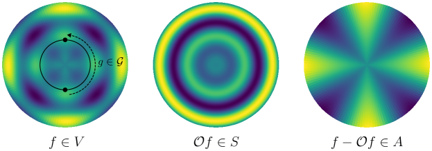
Figure 3.1: Example of a function decomposition. The figure shows $f(r,\theta)=r\cos{(r-2\theta)}\cos{(r+2\theta)}$ decomposed into its $\mathcal{G}$-symmetric and $\mathcal{G}$-anti-symmetric parts in $V=S\oplus A$ under the natural action of $\mathcal{G}=\mathsf{SO}_{2}$ on $\mathbb{R}^{2}$. See Example 3.2. Image credit: Sheheryar Zaidi. Best viewed in colour.

Remark 3.3.

[175] discuss generalising Lemma 3.1 to the non-compact group of scalings $x\mapsto cx$ and demonstrate the impossibility of doing so for real (as opposed to complex) $c$.

3.1.1 Proof of Lemma 3.1

In this section we derive the following result.

Lemma (Lemma 3.1).

Let $U$ be any subspace of ${L_{2}(\mathcal{X},\mathcal{Y},\mu)}$ that is closed under $\mathcal{Q}$, meaning $\mathcal{Q}U\subset U$. Define the subspaces $S$ and $A$ of $U$ consisting of the $\mathcal{G}$-symmetric and $\mathcal{G}$-anti-symmetric functions respectively, $S=\{f\in U:\text{$f$ is $\mathcal{G}$-equivariant}\}$ and $A=\{f\in U:\mathcal{Q}f=0\}$. Then $U$ admits the orthogonal decomposition $U=S\oplus A$.

We first check that $\mathcal{Q}$ is well-defined.

Proposition 3.4.

Let $f\in{L_{2}(\mathcal{X},\mathcal{Y},\mu)}$, then

1. $\mathcal{Q}f$ is $\mu$-measurable, and

2. $\mathcal{Q}f\in{L_{2}(\mathcal{X},\mathcal{Y},\mu)}$ with $\lVert\mathcal{Q}f\rVert_{\mu}\leq\lVert f\rVert_{\mu}$.

Proof.

The mapping $m:(g,x)\mapsto g^{-1}f(gx)\in\mathcal{Y}$ is $(\lambda\otimes\mu)$-measurable by considering the following composition and applying Lemma A.1

$$(g,x)\mapsto(g,gx)\mapsto(g,f(gx))\mapsto g^{-1}f(gx).$$

The lemma requires that each co-ordinate of each tuple is generated by a measurable mapping of the previous tuple, which is true either by assumption or trivially for $(g,x)\mapsto g$.

Lemma A.1 also allows us to verify the $\mu$-measurability of $\mathcal{Q}f$ component-wise. By Corollary A.4, it’s sufficient to verify that each component of $m$ is $(\lambda\otimes\mu)$-integrable. Consider, using Fubini’s theorem, the unitarity of $\psi$ and invariance of $\mu$

$$\int_{\mathcal{G}}\int_{\mathcal{X}}\lVert m(g,x)\rVert^{2}\mathop{}\!\mathrm{d}\mu(x)\mathop{}\!\mathrm{d}\lambda(g) =\int_{\mathcal{G}}\int_{\mathcal{X}}\lVert g^{-1}f(gx)\rVert^{2}\mathop{}\!\mathrm{d}\mu(x)\mathop{}\!\mathrm{d}\lambda(g)$$

$$=\int_{\mathcal{G}}\int_{\mathcal{X}}\lVert f(gx)\rVert^{2}\mathop{}\!\mathrm{d}\mu(x)\mathop{}\!\mathrm{d}\lambda(g)$$

$$=\int_{\mathcal{X}}\lVert f(x)\rVert^{2}\mathop{}\!\mathrm{d}\mu(x)$$

$$=\lVert f\rVert_{\mu}^{2}<\infty$$

so that each component of $m$ is in $L_{2}(\lambda\otimes\mu)$. Theorem 1.1 gives $L_{2}(\lambda\otimes\mu)\subset L_{1}(\lambda\otimes\mu)$ because $\lambda\otimes\mu$ is bounded.

So far we have established the first assertion in the statement, we now verify that $\mathcal{Q}f\in{L_{2}(\mathcal{X},\mathcal{Y},\mu)}$. In Eq. a we use Fubini’s theorem which we will justify at the end of the proof, in Eq. b we use unitarity and in Eq. c we use the invariance of $\mu$ and $\lambda$

$$\lVert\mathcal{Q}f\rVert^{2}_{\mu} =\int_{\mathcal{X}}\left\langle\int_{\mathcal{G}}g_{1}^{-1}f(g_{1}x)\mathop{}\!\mathrm{d}\lambda(g_{1}),\int_{\mathcal{G}}g_{2}^{-1}f(g_{2}x)\mathop{}\!\mathrm{d}\lambda(g_{2})\right\rangle\mathop{}\!\mathrm{d}\mu(x)$$

$$=\int_{\mathcal{X}}\int_{\mathcal{G}}\int_{\mathcal{G}}\left\langle g_{1}^{-1}f(g_{1}x),g_{2}^{-1}f(g_{2}x)\right\rangle\mathop{}\!\mathrm{d}\lambda(g_{1})\mathop{}\!\mathrm{d}\lambda(g_{2})\mathop{}\!\mathrm{d}\mu(x)$$

$$=\int_{\mathcal{G}}\int_{\mathcal{G}}\int_{\mathcal{X}}\left\langle g_{1}^{-1}f(g_{1}x),g_{2}^{-1}f(g_{2}x)\right\rangle\mathop{}\!\mathrm{d}\mu(x)\mathop{}\!\mathrm{d}\lambda(g_{1})\mathop{}\!\mathrm{d}\lambda(g_{2})$$ (a)

$$=\int_{\mathcal{G}}\int_{\mathcal{G}}\int_{\mathcal{X}}\left\langle f(g_{1}x),(g_{2}g_{1}^{-1})^{-1}f(g_{2}x)\right\rangle\mathop{}\!\mathrm{d}\mu(x)\mathop{}\!\mathrm{d}\lambda(g_{1})\mathop{}\!\mathrm{d}\lambda(g_{2})$$ (b)

$$=\int_{\mathcal{G}}\int_{\mathcal{X}}\left\langle f(x),g^{-1}f(gx)\right\rangle\mathop{}\!\mathrm{d}\mu(x)\mathop{}\!\mathrm{d}\lambda(g)$$ (c)

$$=\int_{\mathcal{G}}\langle f,g^{-1}\circ f\circ g\rangle_{\mu}\mathop{}\!\mathrm{d}\lambda(g)$$

$$\leq\lVert f\rVert_{\mu}\int_{\mathcal{G}}\lVert g^{-1}\circ f\circ g\rVert_{\mu}\mathop{}\!\mathrm{d}\lambda(g).$$

It remains to show that $\lVert g^{-1}\circ f\circ g\rVert_{\mu}=\lVert f\rVert_{\mu}$. For all $g\in\mathcal{G}$,

$$\lVert g^{-1}\circ f\circ g\rVert_{\mu}^{2} =\int_{\mathcal{X}}\langle g^{-1}f(gx),g^{-1}f(gx)\rangle\mathop{}\!\mathrm{d}\mu(x)$$

$$=\int_{\mathcal{X}}\langle f(gx),f(gx)\rangle\mathop{}\!\mathrm{d}\mu(x)$$

$$=\int_{\mathcal{X}}\langle f(x),f(x)\rangle\mathop{}\!\mathrm{d}\mu(x)$$

$$=\lVert f\rVert_{\mu}^{2}.$$

We now justify Eq. a. To apply Fubini’s theorem we need each $\mathcal{G}$-section of the integrand to be $(\lambda\otimes\mu)$-integrable, for which Proposition 3.5 is sufficient. ∎

Proposition 3.5.

For all $h,f\in{L_{2}(\mathcal{X},\mathcal{Y},\mu)}$ the function $\langle h(x),g^{-1}f(gx)\rangle$ is $(\lambda\otimes\mu)$-integrable.

Proof.

The function is measurable by expanding the inner product in a basis. Then by Cauchy-Schwarz and $a^{2}+b^{2}\geq ab$

$$\int_{\mathcal{G}}\int_{\mathcal{X}}|{}\langle h(x),g^{-1}f(gx)\rangle|{}\mathop{}\!\mathrm{d}\mu(x)\mathop{}\!\mathrm{d}\lambda(g)$$

$$\leq\int_{\mathcal{G}}\int_{\mathcal{X}}\lVert h(x)\rVert\lVert g^{-1}f(gx)\rVert\mathop{}\!\mathrm{d}\mu(x)\mathop{}\!\mathrm{d}\lambda(g)$$

$$\leq\int_{\mathcal{G}}\int_{\mathcal{X}}\lVert h(x)\rVert^{2}\mathop{}\!\mathrm{d}\mu(x)\mathop{}\!\mathrm{d}\lambda(g)+\int_{\mathcal{G}}\int_{\mathcal{X}}\lVert g^{-1}f(gx)\rVert^{2}\mathop{}\!\mathrm{d}\mu(x)\mathop{}\!\mathrm{d}\lambda(g)$$

$$=\lVert h\rVert_{\mu}^{2}+\lVert f\rVert_{\mu}^{2}$$

$$<\infty$$

where in the last line we use unitarity and the invariance of $\mu$. ∎

Now for the important observation that $\mathcal{Q}$ identifies equivariance, as well as enforcing it. If there are any equivariant functions in ${L_{2}(\mathcal{X},\mathcal{Y},\mu)}$ then in combination with Proposition 3.4 this shows that $\mathcal{Q}$ has unit operator norm.

Proposition 3.6.

$f$ is equivariant if and only if $\mathcal{Q}f=f$.

Proof.

Recall that $f$ is equivariant if $f(gx)=gf(x)$ for all $g\in\mathcal{G}$ and all $x\in\mathcal{X}$. Suppose $f$ is equivariant then for all $x\in\mathcal{X}$

$$\mathcal{Q}f(x)=\int_{\mathcal{G}}g^{-1}f(gx)\mathop{}\!\mathrm{d}\lambda(g)=\int_{\mathcal{G}}g^{-1}gf(x)\mathop{}\!\mathrm{d}\lambda(g)=f(x).$$

Now assume that $\mathcal{Q}f=f$, so $f(x)=\int_{\mathcal{G}}g^{-1}f(gx)\mathop{}\!\mathrm{d}\lambda(g)$ for all $x\in\mathcal{X}$. Take any $\tilde{g}\in\mathcal{G}$, then

$$f(\tilde{g}x) =\int_{\mathcal{G}}g^{-1}f(g\tilde{g}x)\mathop{}\!\mathrm{d}\lambda(g)=\tilde{g}\int_{\mathcal{G}}(g\tilde{g})^{-1}f(g\tilde{g}x)\mathop{}\!\mathrm{d}\lambda(g)=\tilde{g}\int_{\mathcal{G}}g^{-1}f(gx)\mathop{}\!\mathrm{d}\lambda(g)$$

$$=\tilde{g}f(x)$$

where in the third equality we used the invariance of the Haar measure. ∎

By Proposition 3.6, $\mathcal{Q}^{2}f=\mathcal{Q}f$ so $\mathcal{Q}$ is a projection. The operator $\mathcal{Q}$ is also linear. Let $U$ be a subspace of ${L_{2}(\mathcal{X},\mathcal{Y},\mu)}$ such that $\mathcal{Q}U\subset U$. Set $S=\mathcal{Q}U$ and $A=(\operatorname{\operatorname{id}}-\mathcal{Q})U$. $S\subset U$, $A\subset U$ and $S\cap A$ is trivial, so $S\oplus A\subset U$. Any $f\in U$ can be written uniquely as $f=\bar{f}+f^{\scaleobj{0.75}{\perp}}$ where $\bar{f}=\mathcal{Q}f$ and $f^{\scaleobj{0.75}{\perp}}=f-\mathcal{Q}f$, so $U\subset S\oplus A$. Hence $U=S\oplus A$. Proposition 3.6 gives $S=\{f\in U:\text{$f$ is $\mathcal{G}$-equivariant}\}$ and $A=\{f\in U:\mathcal{Q}f=0\}$ is easily established: $\mathcal{Q}A=\{0\}$ by linearity and idempotence, while any $f$ with $\mathcal{Q}f=0$ has $f=(\operatorname{\operatorname{id}}-\mathcal{Q})f$. Next we show that $\mathcal{Q}$ is self-adjoint with respect to $\langle\cdot,\cdot\rangle_{\mu}$ which shows that $\mathcal{Q}$ is an orthogonal projection. The orthogonality in Lemma 3.1 follows immediately, since if $f\in S$ and $h\in A$ then

$$\langle f,h\rangle_{\mu}=\langle\mathcal{Q}f,h\rangle_{\mu}=\langle f,\mathcal{Q}h\rangle_{\mu}=\langle f,0\rangle_{\mu}=0.$$

Proposition 3.7.

$\mathcal{Q}$ is self-adjoint with respect to $\langle\cdot,\cdot\rangle_{\mu}$.

Proof.

At various points we apply Fubini’s theorem, the unitarity of $\psi$, the invariance of $\mu$ and use the change of variables $g\mapsto g^{-1}$. The application of Fubini’s theorem is valid by Proposition 3.5. The inner product on $\mathcal{Y}$ commutes with integration (e.g., by expanding in a basis). Let $f,h\in{L_{2}(\mathcal{X},\mathcal{Y},\mu)}$, then

$$\langle\mathcal{Q}f,h\rangle_{\mu} =\int_{\mathcal{X}}\left\langle\int_{\mathcal{G}}g^{-1}f(gx)\mathop{}\!\mathrm{d}\lambda(g),h(x)\right\rangle\mathop{}\!\mathrm{d}\mu(x)$$

$$=\int_{\mathcal{X}}\int_{\mathcal{G}}\langle g^{-1}f(gx),h(x)\rangle\mathop{}\!\mathrm{d}\lambda(g)\mathop{}\!\mathrm{d}\mu(x)$$

$$=\int_{\mathcal{G}}\int_{\mathcal{X}}\langle g^{-1}f(gx),h(x)\rangle\mathop{}\!\mathrm{d}\mu(x)\mathop{}\!\mathrm{d}\lambda(g)$$

$$=\int_{\mathcal{G}}\int_{\mathcal{X}}\langle f(x),gh(g^{-1}x)\rangle\mathop{}\!\mathrm{d}\mu(x)\mathop{}\!\mathrm{d}\lambda(g)$$

$$=\int_{\mathcal{X}}\left\langle f(x),\int_{\mathcal{G}}gh(g^{-1}x)\mathop{}\!\mathrm{d}\lambda(g)\right\rangle\mathop{}\!\mathrm{d}\mu(x)$$

$$=\int_{\mathcal{X}}\left\langle f(x),\int_{\mathcal{G}}g^{-1}h(gx)\mathop{}\!\mathrm{d}\lambda(g)\right\rangle\mathop{}\!\mathrm{d}\mu(x)$$

$$=\langle f,\mathcal{Q}h\rangle_{\mu}.$$

∎

3.1.2 The invariance of $\mu$

The invariance of $\mu$ is used throughout the proof of Lemma 3.1. There are many tasks for which invariance of the input distribution is a natural assumption, for instance in medical imaging [188], but the reader may wonder whether it is necessary for our results. In the following example from Sheheryar Zaidi, invariance is equivalent to the orthogonality in the decomposition ${L_{2}(\mathcal{X},\mathcal{Y},\mu)}=S\oplus A$. This means invariance is necessary for Lemma 3.1 to hold in general. An alternative phrasing is that the projection $\mathcal{Q}$ is only orthogonal in the below setting if $\mu$ is invariant. Note that in the example below $\psi$ is the trivial representation.

Example 3.8 (Sheheryar Zaidi [52]).

Let $\mathsf{C}_{2}$ act on $\mathcal{X}=\{-1,1\}\times\{1\}$ by multiplication on the first coordinate. Let $V$ be the vector space of functions $f_{(t_{1},t_{2})}:\mathcal{X}\to\mathbb{R}$ with $f_{(t_{1},t_{2})}(x_{1},x_{2})=t_{1}x_{1}+t_{2}x_{2}$ for all $t_{1},t_{2}\in\mathbb{R}$. We note that any distribution $\mu$ on $\mathcal{X}$ can be described by its probability mass function $p$, which is defined by $p(-1,1)$ and $p(1,1)$. Moreover, $\mu$ is $\mathsf{C}_{2}$-invariant if and only if $p(-1,1)=p(1,1)$. Next, observe that the $\mathcal{G}$-symmetric functions $S$ and $\mathcal{G}$-anti-symmetric functions $A$ are precisely those for which $t_{1}=0$ and $t_{2}=0$ respectively. The inner product induced by $\mu$ is given by $\langle f_{(a_{1},a_{2})},f_{(b_{1},b_{2})}\rangle_{\mu}=(a_{1}+a_{2})(b_{1}+b_{2})p(1,1)+(a_{2}-a_{1})(b_{2}-b_{1})p(-1,1)$. With this, we see that the inner product $\langle f_{(0,t_{2})},f_{(t_{1},0)}\rangle_{\mu}=t_{1}t_{2}p(1,1)-t_{1}t_{2}p(-1,1)$ is zero for all $f_{(0,t_{2})}\in S$ and $f_{(t_{1},0)}\in A$ if and only if $p(-1,1)=p(1,1)$. That is, if and only if $\mu$ is invariant.

3.2 Warm Up

In this section we consider some basic consequences of Lemma 3.1 and of our setup more generally. Recall the special case of $\mathcal{Q}$ where $\psi$ is the trivial representation, corresponding to invariance rather than equivariance,

$$\mathcal{O}f(x)=\int_{\mathcal{G}}f(gx)\mathop{}\!\mathrm{d}\lambda(g).$$

3.2.1 Feature Averaging as a Least Squares Problem

When $f$ is a feature extractor, e.g., the final layer representations of a neural network, $\mathcal{O}$ can be thought of as performing feature averaging. Using Lemma 3.1, feature averaging can be viewed as solving a least squares problem in ${L_{2}(\mathcal{X},\mathcal{Y},\mu)}$. That is, feature averaging sends $f$ to $\bar{f}$ where $\bar{f}$ is the closest invariant feature extractor to $f$. This just a well known fact about orthogonal projections written in different terms, but we give a proof for completeness. The same result holds for $\mathcal{Q}$.

Proposition 3.1.

Define $S$ and $A$ as in Lemma 3.1. For all $f\in{L_{2}(\mathcal{X},\mathcal{Y},\mu)}$, feature averaging with $\mathcal{O}$ maps $f\mapsto\bar{f}$ where $\bar{f}$ is the unique solution to the least squares problem $\bar{f}=\operatorname*{argmin}_{s\in S}\lVert f-s\rVert^{2}_{\mu}$.

Proof.

By Lemma 3.1 we can write $f=\bar{f}+f^{\scaleobj{0.75}{\perp}}$ where $\bar{f}=\mathcal{O}f\in S$, $f^{\scaleobj{0.75}{\perp}}\in A$ and the two terms are orthogonal. Take any $h\in S$, then using the orthogonality

$$\lVert f-h\rVert_{\mu}^{2}=\lVert(\bar{f}-h)+f^{\scaleobj{0.75}{\perp}}\rVert_{\mu}^{2}=\lVert\bar{f}-h\rVert_{\mu}^{2}+\lVert f^{\scaleobj{0.75}{\perp}}\rVert_{\mu}^{2}\geq\lVert f^{\scaleobj{0.75}{\perp}}\rVert_{\mu}^{2}=\lVert f-\bar{f}\rVert_{\mu}^{2}.$$

Set $s=\bar{f}$ and suppose $\exists s^{\prime}\in S$ with $s^{\prime}\neq s$ and $\lVert f-s^{\prime}\rVert_{\mu}=\lVert f-s\rVert_{\mu}$, then since $S$ is a vector space we have $s_{\frac{1}{2}}=\frac{1}{2}(s+s^{\prime})\in S$. It follows, using Cauchy-Schwarz, that

$$\lVert f-s_{\frac{1}{2}}\rVert_{\mu}^{2} =\lVert(f-s)/2+(f-s^{\prime})/2\rVert_{\mu}^{2}$$

$$=\frac{1}{4}\lVert f-s\rVert_{\mu}^{2}+\frac{1}{4}\lVert f-s^{\prime}\rVert_{\mu}^{2}+\frac{1}{4}\langle f-s,f-s^{\prime}\rangle_{\mu}$$

$$\leq\frac{1}{4}\lVert f-s\rVert_{\mu}^{2}+\frac{1}{4}\lVert f-s\rVert_{\mu}^{2}+\frac{1}{4}\lVert f-s\rVert_{\mu}^{2}$$

$$=\frac{3}{4}\lVert f-s\rVert_{\mu}^{2},$$

which a contradiction unless $\lVert f-s\rVert_{\mu}^{2}=0$, in which case $f=s$ in ${L_{2}(\mathcal{X},\mathcal{Y},\mu)}$. ∎

Example 3.2.

Consider again the setting of Example 3.2. For simplicity, let $f(r,\theta)=f_{\text{rad}}(r)f_{\text{ang}}(\theta)$ be separable in polar coordinates. Notice that $\mathcal{O}f=c_{f}f_{\text{rad}}$ where $c_{f}=\frac{1}{2\pi}\int_{0}^{2\pi}f_{\text{ang}}(\theta)\mathop{}\!\mathrm{d}\theta$. Then for any $s\in S$ we can calculate:

$$\lVert f-s\rVert_{\mu}^{2} =\frac{1}{2\pi}\int_{\mathcal{X}}(f(r,\theta)-s(r))^{2}\mathsf{e}^{-r^{2}/2}r\mathop{}\!\mathrm{d}r\mathop{}\!\mathrm{d}\theta$$

$$=\frac{1}{2\pi}\int_{\mathcal{X}}(f(r,\theta)-c_{f}f_{\text{rad}}(r))^{2}\mathsf{e}^{-r^{2}/2}r\mathop{}\!\mathrm{d}r\mathop{}\!\mathrm{d}\theta$$

$$\phantom{=}+\frac{1}{2\pi}\int_{\mathcal{X}}(c_{f}f_{\text{rad}}(r)-s(r))^{2}\mathsf{e}^{-r^{2}/2}r\mathop{}\!\mathrm{d}r\mathop{}\!\mathrm{d}\theta$$

which is minimised by $s=c_{f}f_{\text{rad}}$.

3.2.2 Averaging and the Rademacher Complexity

Let $T=(x_{1},\dots,x_{n})$ be a collection of points from $\mathcal{X}$. The empirical Rademacher complexity of a set $\mathcal{F}$ of functions $f:\mathcal{X}\to\mathbb{R}$ evaluated on $T$ is defined by

$$\operatorname{\widehat{\mathfrak{R}}}_{T}(\mathcal{F})=\operatorname{\mathbb{E}}\left[\sup_{f\in\mathcal{F}}\left|{}\frac{1}{n}\sum_{i=1}^{n}\varsigma_{i}f(x_{i})\right|{}\right]$$

where the expectation is over the random variables $\varsigma_{i}\sim\operatorname{\operatorname{Unif}}\{-1,1\}$ which follow the Rademacher distribution. If the $T$ is random then the empirical Rademacher complexity $\operatorname{\widehat{\mathfrak{R}}}_{T}(\mathcal{F})$ is a random quantity and the Rademacher complexity $\operatorname{\mathfrak{R}}_{n}(\mathcal{F})$ is defined by $\operatorname{\mathfrak{R}}_{n}(\mathcal{F})=\operatorname{\mathbb{E}}[\operatorname{\widehat{\mathfrak{R}}}_{T}(\mathcal{F})]$. The Rademacher complexity appears in the study of generalisation in statistical learning, for instance see [182, Theorem 4.10 and Proposition 4.12] for upper and lower bounds respectively. A reduction in the Rademacher complexity means that fewer examples are required to achieve a specified worst-case risk.

Let $\mathcal{F}\subset{L_{2}(\mu)}$ and consider its $\mathcal{G}$-symmetric and $\mathcal{G}$-anti-symmetric projections $\overline{\mathcal{F}}=\mathcal{O}\mathcal{F}$ and $\mathcal{F}_{\scaleobj{0.75}{\perp}}=(\operatorname{\operatorname{id}}-\mathcal{O})\mathcal{F}$ respectively. We assume that both versions of the Rademacher complexity are well-defined on $\mathcal{F}$, $\overline{\mathcal{F}}$ and $\mathcal{F}_{\scaleobj{0.75}{\perp}}$.

Proposition 3.3.

The Rademacher complexity of the feature averaged class satisfies

$$0\leq\operatorname{\mathfrak{R}}_{n}(\mathcal{F})-\operatorname{\mathfrak{R}}_{n}(\overline{\mathcal{F}})\leq\operatorname{\mathfrak{R}}_{n}(\mathcal{F}_{\scaleobj{0.75}{\perp}})$$

whenever the terms are finite and where the data are distributed $T\sim\otimes^{n}\mu$.

Proof.

We will show that $\operatorname{\mathfrak{R}}_{n}(\overline{\mathcal{F}})\leq\operatorname{\mathfrak{R}}_{n}(\mathcal{F})\leq\operatorname{\mathfrak{R}}_{n}(\overline{\mathcal{F}})+\operatorname{\mathfrak{R}}_{n}(\mathcal{F}_{\scaleobj{0.75}{\perp}})$, from which the proposition follows immediately. We start by establishing $\operatorname{\mathfrak{R}}_{n}(\overline{\mathcal{F}})\leq\operatorname{\mathfrak{R}}_{n}(\mathcal{F})$. The action of $\mathcal{G}$ on $\mathcal{X}$ induces an action on $\mathcal{X}^{n}$ by $g(x_{1},\dots,x_{n})=(gx_{1},\dots,gx_{n})$ under which $\otimes^{n}\mu$ is invariant. Let $X_{1},\dots,X_{n}\sim\mu$, then note that

$$\operatorname{\mathfrak{R}}_{n}(\overline{\mathcal{F}}) =\frac{1}{n}\operatorname{\mathbb{E}}\left[\sup_{\bar{f}\in\overline{\mathcal{F}}}\left|{}\sum_{i=1}^{n}\varsigma_{i}\bar{f}(X_{i})\right|{}\right]$$

$$=\frac{1}{n}\operatorname{\mathbb{E}}\left[\sup_{f\in\mathcal{F}}\left|{}\sum_{i=1}^{n}\varsigma_{i}\int_{\mathcal{G}}f(gX_{i})\mathop{}\!\mathrm{d}\lambda(g)\right|{}\right]$$

$$\leq\frac{1}{n}\operatorname{\mathbb{E}}\left[\sup_{f\in\mathcal{F}}\int_{\mathcal{G}}\left|{}\sum_{i=1}^{n}\varsigma_{i}f(gX_{i})\right|{}\mathop{}\!\mathrm{d}\lambda(g)\right].$$

We obtain $\operatorname{\mathfrak{R}}_{n}(\overline{\mathcal{F}})\leq\operatorname{\mathfrak{R}}_{n}(\mathcal{F})$ by the fact that the last line above is dominated by Eq. b below

$$\operatorname{\mathfrak{R}}_{n}(\mathcal{F}) =\frac{1}{n}\operatorname{\mathbb{E}}\left[\sup_{f\in\mathcal{F}}\left|{}\sum_{i=1}^{n}\varsigma_{i}f(X_{i})\right|{}\right]$$

$$=\frac{1}{n}\int_{\mathcal{G}}\operatorname{\mathbb{E}}\left[\sup_{f\in\mathcal{F}}\left|{}\sum_{i=1}^{n}\varsigma_{i}f(gX_{i})\right|{}\right]\mathop{}\!\mathrm{d}\lambda(g)$$ (a)

$$=\frac{1}{n}\operatorname{\mathbb{E}}\left[\int_{\mathcal{G}}\sup_{f\in\mathcal{F}}\left|{}\sum_{i=1}^{n}\varsigma_{i}f(gX_{i})\right|{}\mathop{}\!\mathrm{d}\lambda(g)\right].$$ (b)

In Eq. a we used the invariance of $\mu$. In Eq. b we use Fubini’s theorem which also guarantees that the expression is well-defined (although possibly infinite).

We now prove that $\operatorname{\mathfrak{R}}_{n}(\mathcal{F})\leq\operatorname{\mathfrak{R}}_{n}(\overline{\mathcal{F}})+\operatorname{\mathfrak{R}}_{n}(\mathcal{F}_{\scaleobj{0.75}{\perp}})$. For any $f\in\mathcal{F}$ we can write $f=\bar{f}+f^{\scaleobj{0.75}{\perp}}$ where $\bar{f}\in\overline{\mathcal{F}}$ and $f^{\scaleobj{0.75}{\perp}}\in\mathcal{F}_{\scaleobj{0.75}{\perp}}$ by Lemma 3.1. The result follows from taking expectations over $T\sim\otimes^{n}\mu$ of the below. For any $T=(x_{1},\dots,x_{n})$

$$\operatorname{\widehat{\mathfrak{R}}}_{T}(\mathcal{F}) =\frac{1}{n}\operatorname{\mathbb{E}}\left[\sup_{f\in\mathcal{F}}\left|{}\sum_{i=1}^{n}\varsigma_{i}f(x_{i})\right|{}\right]$$

$$=\frac{1}{n}\operatorname{\mathbb{E}}\left[\sup_{f\in\mathcal{F}}\left|{}\sum_{i=1}^{n}(\varsigma_{i}\bar{f}(x_{i})+\varsigma_{i}f^{\scaleobj{0.75}{\perp}}(x_{i}))\right|{}\right]$$

$$\leq\frac{1}{n}\operatorname{\mathbb{E}}\left[\sup_{\bar{f}\in\overline{\mathcal{F}}}\left|{}\sum_{i=1}^{n}\varsigma_{i}\bar{f}(x_{i})\right|{}\right]+\frac{1}{n}\operatorname{\mathbb{E}}\left[\sup_{f^{\scaleobj{0.75}{\perp}}\in\mathcal{F}_{\scaleobj{0.75}{\perp}}}\left|{}\sum_{i=1}^{n}\varsigma_{i}f^{\scaleobj{0.75}{\perp}}(x_{i})\right|{}\right]$$

$$=\operatorname{\widehat{\mathfrak{R}}}_{T}(\overline{\mathcal{F}})+\operatorname{\widehat{\mathfrak{R}}}_{T}(\mathcal{F}_{\scaleobj{0.75}{\perp}})$$

∎

Proposition 3.3 says that the Rademacher complexity is reduced by orbit averaging, but not by more than the complexity of the $\mathcal{G}$-anti-symmetric component of the class. This quantifies the improvement in worst-case generalisation from enforcing invariance by averaging in terms of the extent to which the inductive bias is already present in the function class. We provide stronger results in later sections and chapters, studying individual predictors and the average case for learning algorithms.

3.3 Implications for Generalisation

3.3.1 The Generalisation Gap in Regression Problems

In this section we apply Lemma 3.1 to derive a strict (i.e., non-zero) generalisation gap between predictors that have and have not been specified to have the symmetry that is present in the task.

Given some pair of random elements $(X,Y)$ with values on $\mathcal{X}\times\mathcal{Y}$ defining a supervised learning task (with inputs in $\mathcal{X}$ and outputs in $\mathcal{Y}$), we define the risk of a predictor $f$ as

$$R[f]=\operatorname{\mathbb{E}}[\lVert f(X)-Y\rVert^{2}].$$

This is the same definition of the risk, just specialised to the loss function $\ell(y,y^{\prime})=\lVert y-y^{\prime}\rVert^{2}$, where $\lVert\cdot\rVert$ is the inner product norm on $\mathcal{Y}$. A consequence of the following result is that, on a task with equivariant structure, the difference in risk between a predictor $f$ and any equivariant predictor $f^{\prime}$ such that $R[f^{\prime}]\leq R[\mathcal{Q}f]$ is at least the norm of the $\mathcal{G}$-anti-symmetric component of of $f$. This shows a barrier to generalisation if $f$ is not equivariant. It also shows that the lower bound on the risk can be (approximately) eliminated by making $f$ (approximately) equivariant. In short: for any non-equivariant predictor, there is an equivariant predictor that performs better. The projection $\mathcal{Q}f$ is the archetypal equivariant predictor to which $f$ should be compared. From Lemma 3.1, $\mathcal{Q}f$ can be thought of the equivariant part of $f$ and in addition $\mathcal{Q}f$ is the closest equivariant predictor to $f$.

Lemma 3.1.

Let $X\sim\mu$ and let $Y$ have finite second moment. Assume either of the following models for $Y$

1. $Y\overset{\text{d}}{=}f^{\star}(X)+\xi$ where $f^{\star}\in{L_{2}(\mathcal{X},\mathcal{Y},\mu)}$ is equivariant, $\operatorname{\mathbb{E}}[\xi]=0$ and $\operatorname{\mathbb{E}}[\lVert\xi\rVert^{2}]<\infty$, or

2. $Y\overset{\text{d}}{=}\tilde{f}(X,\eta)$ where $\tilde{f}:\mathcal{X}\times[0,1]\to\mathbb{R}$ is equivariant in its first argument, $\eta\sim\operatorname{\operatorname{Unif}}[0,1]$ and $\eta\perp\!\!\!\perp X$.

Let $f\in{L_{2}(\mathcal{X},\mathcal{Y},\mu)}$ and let $f^{\prime}\in{L_{2}(\mathcal{X},\mathcal{Y},\mu)}$ be any predictor such that $R[f^{\prime}]\leq R[\bar{f}]$ where $\bar{f}=\mathcal{Q}f$. Let $f^{\scaleobj{0.75}{\perp}}=f-\bar{f}$ be the $\mathcal{G}$-anti-symmetric component of $f$, then

$$R[f]-R[f^{\prime}]\geq\lVert f^{\scaleobj{0.75}{\perp}}\rVert_{\mu}^{2}$$

with equality when $R[f^{\prime}]=R[\bar{f}]$.

Proof.

Assume the statement in the case of equality. Consider $f^{\prime}\in{L_{2}(\mathcal{X},\mathcal{Y},\mu)}$ such that $R[f^{\prime}]\leq R[\bar{f}]$, then $R[f]-R[f^{\prime}]=R[f]-R[\bar{f}]+R[\bar{f}]-R[f^{\prime}]\geq\lVert f^{\scaleobj{0.75}{\perp}}\rVert_{\mu}^{2}$. We now address the case of equality for each model. Suppose $Y\overset{\text{d}}{=}f^{\star}(X)+\xi$. Using Lemma 3.1 we write $f=\bar{f}+f^{\scaleobj{0.75}{\perp}}$ where the terms are orthogonal and the first is equivariant. Then using $\operatorname{\mathbb{E}}[\xi]=0$ and the orthogonality

$$R[f] =\operatorname{\mathbb{E}}[\lVert f(X)-Y\rVert^{2}]$$

$$=\operatorname{\mathbb{E}}[\lVert\bar{f}(X)-f^{\star}(X)+f^{\scaleobj{0.75}{\perp}}(X)\rVert^{2}]+\operatorname{\mathbb{E}}[\lVert\xi\rVert^{2}]$$

$$=\lVert\bar{f}-f^{\star}+f^{\scaleobj{0.75}{\perp}}\rVert^{2}_{\mu}+\operatorname{\mathbb{E}}[\lVert\xi\rVert^{2}]$$

$$=\lVert\bar{f}-f^{\star}\rVert_{\mu}^{2}+\lVert f^{\scaleobj{0.75}{\perp}}\rVert^{2}_{\mu}+\operatorname{\mathbb{E}}[\lVert\xi\rVert^{2}]$$

$$=R[\bar{f}]+\lVert f^{\scaleobj{0.75}{\perp}}\rVert^{2}_{\mu}.$$

Now consider the second model for $Y$. Let us write $f^{\star}_{t}(x)=\tilde{f}(x,t)$. Since $Y$ has finite second moment

$$\infty>\operatorname{\mathbb{E}}[\lVert Y\rVert^{2}]=\int_{[0,1]}\lVert f^{\star}_{t}\rVert_{\mu}^{2}\mathop{}\!\mathrm{d}t$$

by Fubini’s theorem so $f^{\star}_{t}\in{L_{2}(\mathcal{X},\mathcal{Y},\mu)}$ for almost all $t\in[0,1]$. As before, we can use Lemma 3.1 to get the orthogonal decomposition $f=\bar{f}+f^{\scaleobj{0.75}{\perp}}$. Additionally, the equivariance of $f^{\star}_{t}$ means $\langle f^{\star}_{t},f^{\scaleobj{0.75}{\perp}}\rangle_{\mu}=0$. Hence

$$R[f]=\operatorname{\mathbb{E}}[\lVert f(X)-Y\rVert^{2}]=\operatorname{\mathbb{E}}[\lVert f-f^{\star}_{\eta}\rVert_{\mu}^{2}]=\operatorname{\mathbb{E}}[\lVert\bar{f}-f^{\star}_{\eta}\rVert_{\mu}^{2}]+\lVert f^{\scaleobj{0.75}{\perp}}\rVert_{\mu}^{2}=R[\bar{f}]+\lVert f^{\scaleobj{0.75}{\perp}}\rVert_{\mu}^{2}.$$

∎

The first model for $Y$ in Lemma 3.1 covers the standard regression setup with an equivariant target function. The second model, inspired by [22], gives conditional equivariance in distribution: $Y|{}gX\overset{\text{d}}{=}gY|{}X$ for all $g\in\mathcal{G}$ and is aimed at stochastic equivariant functions. The first is a special case of the second when $\xi$ is invariant in distribution. Additionally, [22] show that conditional invariance in distribution, i.e., $Y|{}gX\overset{\text{d}}{=}Y|{}X$ for all $g\in\mathcal{G}$, is equivalent to $Y\overset{\text{a.s.}}{=}\tilde{f}(X,\eta)$ for some $\tilde{f}$ that’s invariant in its first argument. It’s straightforward to derive a version of Lemma 3.1 for the case that $f^{\star}$ or $\tilde{f}$ are approximately equivariant.

In later chapters we will use Lemma 3.1 to calculate explicitly the generalisation benefit of invariance/equivariance in random design least squares regression and kernel ridge regression. We will see that $\lVert f^{\scaleobj{0.75}{\perp}}\rVert_{\mu}^{2}$ displays a natural relationship between the number of training examples and the dimension of the space of $\mathcal{G}$-anti-symmetric predictors $A$, which is a property of the group action. Intuitively, the learning algorithm needs enough examples to learn to be orthogonal to $A$.

Remark 3.2.

The same idea used in Lemma 3.1 can be used to give a lower bound on the excess risk in the misspecified case where the predictor $f$ is equivariant but the target $f^{\star}$ is not. For instance, under the first model in Lemma 3.1

$$R[f]-R[f^{\star}]=\lVert f-\mathcal{Q}f^{\star}\rVert_{\mu}^{2}+\lVert(\operatorname{\operatorname{id}}-\mathcal{Q})f^{\star}\rVert_{\mu}^{2}\geq\lVert(\operatorname{\operatorname{id}}-\mathcal{Q})f^{\star}\rVert_{\mu}^{2}.$$

3.3.2 Detour: Test-Time Augmentation

Test-time augmentation consists of averaging the output of a learned function $f$ over random transformations of its input and can be used to increase test accuracy [163, 168, 77]. When the transformations belong to a group $\mathcal{G}$ and are sampled from its Haar measure, test-time augmentation can be written as

$$\widehat{\mathcal{O}}_{n}f(x)=\frac{1}{n}\sum_{i=1}^{n}f(G_{i}x)$$

where $G_{1},\dots,G_{n}\sim\lambda$ are independent and identically distributed. We can view $\widehat{\mathcal{O}}_{n}f$ as an unbiased Monte-Carlo estimate of $\mathcal{O}f$. For any bounded function $f$ and any $x$, $\widehat{\mathcal{O}}f(x)\to\mathcal{O}f(x)$ $\lambda$-almost-surely by the strong law of large numbers [85, Theorem 4.23]. By considering this limit, Lemma 3.1 hints at an explanation for the generalisation improvement from test-time augmentation.

However, more work is needed to connect Lemma 3.1 to [163, 168, 77]. In particular, [163, 168, 77] average softmax outputs rather than predictions and use classification accuracy to calculate the test error.

Chapter 4 The Linear Model

Summary

In this chapter we apply Lemmas 3.1 and 3.1 to linear models in a random design setting. Although invariance is a special case of equivariance, we find it instructive to discuss separately the fully general result of least squares regression with an equivariant target and the special case of an invariant, scalar valued target. These results are given in Theorems 4.4 and 4.1 respectively. The work in this chapter provides the first proofs of a strict generalisation benefit of invariance/equivariance in each case.

Notation

In this chapter we will write the actions $\phi$ and $\psi$ explicitly. In particular we write

$$\mathcal{Q}f(x)=\int_{\mathcal{G}}\psi(g^{-1})f(\phi(g)x)\mathop{}\!\mathrm{d}\lambda(g),$$

and analogously for $\mathcal{O}$.

4.1 Regression with an Invariant Target

Let $\mathcal{X}=\mathbb{R}^{d}$ with the Euclidean inner product and $\mathcal{Y}=\mathbb{R}$ with multiplication. Consider linear regression with the squared-error loss $\ell(y,y^{\prime})=(y-y^{\prime})^{2}$. Let $\mathcal{G}$ act on $\mathcal{X}$ via an orthogonal representation $\phi:\mathcal{G}\to\mathsf{O}_{d}$ and let $X\sim\mu$ be such that $\Sigma\coloneqq\operatorname{\mathbb{E}}[XX^{\top}]$ is finite and positive definite. We consider linear predictors $h_{w}:\mathcal{X}\to\mathcal{Y}$ with $h_{w}(x)=w^{\top}x$ where $w\in\mathcal{X}$. Define the space of all linear predictors $V_{\text{lin}}=\{h_{w}:w\in\mathcal{X}\}$ which is a subspace of ${L_{2}(\mu)}$. Notice that $V_{\text{lin}}$ is closed under $\mathcal{O}$: for all $x\in\mathcal{X}$

$$\mathcal{O}h_{w}(x) =\int_{\mathcal{G}}h_{w}(gx)\mathop{}\!\mathrm{d}\lambda(g)$$

$$=\int_{\mathcal{G}}w^{\top}\phi(g)x\mathop{}\!\mathrm{d}\lambda(g)$$

$$=\left(\int_{\mathcal{G}}\phi(g^{-1})w\mathop{}\!\mathrm{d}\lambda(g)\right)^{\top}x$$

$$=h_{\Phi(w)}(x)$$

where we substituted $g\mapsto g^{-1}$ and defined the linear map $\Phi:\mathbb{R}^{d}\to\mathbb{R}^{d}$ by $\Phi(w)=\int_{\mathcal{G}}\phi(g)w\mathop{}\!\mathrm{d}\lambda(g)$. We also have

$$\langle h_{a},h_{b}\rangle_{\mu}=\int_{\mathcal{X}}a^{\top}xx^{\top}b\mathop{}\!\mathrm{d}\mu(x)=a^{\top}\Sigma b.$$

We denote the induced inner product on $\mathcal{X}$ by $\langle a,b\rangle_{\Sigma}\coloneqq a^{\top}\Sigma b$ and the corresponding norm by $\lVert\cdot\rVert_{\Sigma}$. Since $V_{\text{lin}}$ is closed under $\mathcal{O}$ we can apply Lemma 3.1 to decompose $V_{\text{lin}}=S\oplus A$ with the orthogonality with respect to $\langle\cdot,\cdot\rangle_{\Sigma}$. It follows that we can write any $h_{w}\in V_{\text{lin}}$ as

$$h_{w}=\overline{h_{w}}+h_{w}^{\scaleobj{0.75}{\perp}}$$

where we have shown that there must exist $\bar{w},w^{\scaleobj{0.75}{\perp}}\in\mathcal{X}$ with $\langle\bar{w},w^{\scaleobj{0.75}{\perp}}\rangle_{\Sigma}=0$ such that $\overline{h_{w}}=h_{\bar{w}}$ and $h_{w}^{\scaleobj{0.75}{\perp}}=h_{w^{\scaleobj{0.75}{\perp}}}$. There is an isomorphism $\mathcal{X}\to V_{\text{lin}}$ where $w\mapsto h_{w}$. Using this identification, we abuse notation slightly and write $\mathcal{X}=S\oplus A$ to represent the induced structure on $\mathcal{X}$.

Recall the definition of the risk of a predictor $f$

$$R[f]=\operatorname{\mathbb{E}}[\lVert f(X)-Y\rVert^{2}].$$

The risk is implicitly conditional on any randomness in $f$, e.g., occurring from its dependence on training data. We will refer to the difference in risk between two predictors as the generalisation gap. So the generalisation gap between $f$ and $f^{\prime}$ is $R[f]-R[f^{\prime}]$. If this quantity is positive, then we have strictly better test performance from $f^{\prime}$. This gives a method of comparing predictors.

Suppose examples are labelled by a target function $h_{\theta}\in V_{\text{lin}}$ that is $\mathcal{G}$-invariant. Let $X\sim\mu$ and $Y=\theta^{\top}X+\xi$ where $\xi$ is independent of $X$, has mean 0 and finite variance. We calculate the difference in risk between $h_{w}$ and its invariant version $h_{\bar{w}}$. Lemma 3.1 gives

$$R[h_{w}]-R[h_{\bar{w}}]=\lVert h_{w^{\scaleobj{0.75}{\perp}}}\rVert_{\mu}^{2}=\lVert w^{\scaleobj{0.75}{\perp}}\rVert_{\Sigma}^{2}$$ (4.1.1)

In Theorem 4.1 we calculate this quantity exactly. where $w$ is the minimum-norm least squares estimator and $\bar{w}=\Phi_{\mathcal{G}}(w)$. To the best of our knowledge, this is the first result to specify the generalisation benefit of invariant models.

Theorem 4.1.

Let $\mathcal{X}=\mathbb{R}^{d}$, $\mathcal{Y}=\mathbb{R}$ and let $\mathcal{G}$ be a compact group with an orthogonal representation $\phi$ on $\mathcal{X}$. Let $X\sim\operatorname{\mathcal{N}}(0,\sigma_{X}^{2}I)$ and $Y=h_{\theta}(X)+\xi$ where $h_{\theta}(x)=\theta^{\top}x$ is $\mathcal{G}$-invariant with $\theta\in\mathbb{R}^{d}$ and where $\xi$ has mean $0$, variance $\sigma_{\xi}^{2}<\infty$ and is independent of $X$. Let $w$ be the least squares estimate of $\theta$ from i.i.d. training examples $((X_{i},Y_{i}):i=1,\dots,n)$ distributed independently of and identically to $(X,Y)$ and let $A$ be the orthogonal complement of the subspace of $\mathcal{G}$-invariant linear predictors (as in Lemma 3.1).

• If $n>d+1$ then the generalisation gap satisfies

  $$\operatorname{\mathbb{E}}\left[R[h_{w}]-R[h_{\bar{w}}]\right]=\sigma_{\xi}^{2}\frac{\dim A}{n-d-1}.$$

• At the interpolation threshold $n\in[d-1,d+1]$, if $h_{w}$ is not $\mathcal{G}$-invariant then the generalisation gap diverges to $\infty$.

• If $n<d-1$ the generalisation gap is

  $$\operatorname{\mathbb{E}}\left[R[h_{w}]-R[h_{\bar{w}}]\right]=\dim A\left(\sigma_{X}^{2}\lVert\theta\rVert_{2}^{2}\frac{n(d-n)}{d(d-1)(d+2)}+\sigma_{\xi}^{2}\frac{n}{d(d-n-1)}\right).$$

The expectations are over the training sample. All of the above hold with $\geq$ when $h_{\bar{w}}$ is replaced by any predictor $h^{\prime}$ such that $R[h^{\prime}]\leq R[h_{\bar{w}}]$ (see Lemma 3.1).

Proof.

Note that $X$ is $\mathcal{G}$-invariant for all $\mathcal{G}$ since the representation $\phi$ is orthogonal. We have seen above that the space of linear maps $V_{\text{lin}}=\{h_{w}:w\in\mathbb{R}^{d}\}$ is closed under $\mathcal{O}$, so by Lemma 3.1 we can write $V_{\text{lin}}=S\oplus A$. Let $\Phi^{A}=I-\Phi$, which is the orthogonal projection onto the subspace $A$. By isotropy of $X$ and Eq. 4.1.1 we have

$$R[h_{w}]-R[h_{\bar{w}}]=\sigma_{X}^{2}\lVert w^{\scaleobj{0.75}{\perp}}\rVert_{2}^{2}$$

for all $w\in\mathbb{R}^{d}$, where $w^{\scaleobj{0.75}{\perp}}=\Phi^{A}(w)$. The proof consists of calculating this quantity in the case that $w$ is the least squares estimator.

Let $\bm{X}\in\mathbb{R}^{n\times d}$ and $\bm{Y}\in\mathbb{R}^{n}$ correspond to row-stacked training examples drawn i.i.d. as in the statement, so $\bm{X}_{ij}=(X_{i})_{j}$ and $\bm{Y}_{i}=Y_{i}$. Similarly, set $\bm{\xi}=\bm{X}\theta-\bm{Y}$. The least squares estimate is the minimum norm solution of $\operatorname*{argmin}_{u\in\mathbb{R}^{d}}\lVert\bm{Y}-\bm{X}u\rVert_{2}^{2}$, i.e.,

$$w=(\bm{X}^{\top}\bm{X})^{+}\bm{X}^{\top}\bm{X}\theta+(\bm{X}^{\top}\bm{X})^{+}\bm{X}^{\top}\bm{\xi}$$ (4.1.2)

where $(\cdot)^{+}$ denotes the Moore-Penrose pseudo-inverse. Define $P_{E}=(\bm{X}^{\top}\bm{X})^{+}\bm{X}^{\top}\bm{X}$, which is an orthogonal projection onto $E$, the rank of $\bm{X}^{\top}\bm{X}$ (this can be seen by diagonalising).

We first calculate $\operatorname{\mathbb{E}}[\lVert w^{\scaleobj{0.75}{\perp}}\rVert_{2}^{2}\mid{}\bm{X}]$ where $w^{\scaleobj{0.75}{\perp}}=\Phi^{A}(w)$. The contribution from the first term of Eq. 4.1.2 is

$$\lVert\Phi^{A}(P_{E}\theta)\rVert_{2}^{2},$$

the cross term vanishes using $\xi\perp\!\!\!\perp X$ and $\operatorname{\mathbb{E}}[\xi]=0$, and the contribution from the second term of Eq. 4.1.2 is

$$\operatorname{\mathbb{E}}[\lVert\Phi^{A}((\bm{X}^{\top}\bm{X})^{+}\bm{X}^{\top}\bm{\xi})\rVert_{2}^{2}\mid{}\bm{X}].$$

$\Phi^{A}$ is an orthogonal projection, so as a matrix is symmetric and idempotent. Hence, briefly writing $\Phi^{A}$ without the parenthesis to emphasise the matrix interpretation,

$$\operatorname{\mathbb{E}}[\lVert\Phi^{A}((\bm{X}^{\top}\bm{X})^{+}\bm{X}^{\top}\bm{\xi})\rVert_{2}^{2}\mid{}\bm{X}] =\operatorname{\mathbb{E}}[\operatorname{Tr}(\bm{\xi}^{\top}\bm{X}(\bm{X}^{\top}\bm{X})^{+}\Phi^{A}(\bm{X}^{\top}\bm{X})^{+}\bm{X}^{\top}\bm{\xi})\mid{}\bm{X}]$$

$$=\operatorname{Tr}(\bm{X}(\bm{X}^{\top}\bm{X})^{+}\Phi^{A}(\bm{X}^{\top}\bm{X})^{+}\bm{X}^{\top}\operatorname{\mathbb{E}}[\bm{\xi}\bm{\xi}^{\top}])$$

$$=\sigma_{\xi}^{2}\operatorname{Tr}(\Phi^{A}(\bm{X}^{\top}\bm{X})^{+}).$$

We have obtained

$$\operatorname{\mathbb{E}}[\lVert w^{\scaleobj{0.75}{\perp}}\rVert_{2}^{2}\mid{}\bm{X}]=\lVert\Phi^{A}(P_{E}\theta)\rVert_{2}^{2}+\sigma_{\xi}^{2}\operatorname{Tr}(\Phi^{A}((\bm{X}^{\top}\bm{X})^{+}))$$

and conclude by taking expectations, treating each term separately.

First Term

If $n\geq d$ then $\dim E=d$ with probability $1$, so the first term vanishes almost surely because $\Phi^{A}(\theta)=0$. We treat the $n<d$ case using Einstein notation, in which repeated indices are implicitly summed over. In components, recalling that $\Phi^{A}$ is a matrix,

$$\operatorname{\mathbb{E}}[\lVert\Phi^{A}(P_{E}\theta)\rVert_{2}^{2}]=\Phi^{A}_{fa}\Phi^{A}_{fc}\operatorname{\mathbb{E}}[P_{E}\otimes P_{E}]_{abce}\theta_{b}\theta_{e}$$

and applying Lemma A.6 we get

$$\operatorname{\mathbb{E}}[\lVert\Phi^{A}(P_{E}\theta)\rVert_{2}^{2}] =\frac{n(d-n)}{d(d-1)(d+2)}\left(\Phi^{A}_{fa}\Phi^{A}_{fa}\theta_{b}\theta_{b}+\Phi^{A}_{fa}\Phi^{A}_{fb}\theta_{b}\theta_{a}\right)$$

$$\phantom{=}+\frac{n(d-n)+n(n-1)(d+2)}{d(d-1)(d+2)}\Phi^{A}_{fa}\Phi^{A}_{fc}\theta_{a}\theta_{c}$$

$$=\lVert\theta\rVert_{2}^{2}\dim A\frac{n(d-n)}{d(d-1)(d+2)}$$

where we have used that $\Phi^{A}(\theta)=0$ and $\lVert\Phi^{A}\rVert_{\text{F}}^{2}=\dim A$.

Second Term

By linearity,

$$\operatorname{\mathbb{E}}[\operatorname{Tr}(\Phi^{A}((\bm{X}^{\top}\bm{X})^{+}))]=\operatorname{Tr}(\Phi^{A}(\operatorname{\mathbb{E}}[(\bm{X}^{\top}\bm{X})^{+}])).$$

Then Lemmas A.4 and A.2 give $\operatorname{\mathbb{E}}[(\bm{X}^{\top}\bm{X})^{+}]=\sigma_{X}^{-2}r(n,d)I_{d}$ where

$$r(n,d)=\begin{cases}{\frac{n}{d(d-n-1)}}&n<d-1\\ (n-d-1)^{-1}&n>d+1\\ \infty&\text{otherwise}\end{cases}.$$

When $n\in[d-1,d+1]$ it is well known that the expectation diverges, see Section A.3.1. Hence

$$\operatorname{\mathbb{E}}[\operatorname{Tr}(\Phi^{A}((\bm{X}^{\top}\bm{X})^{+}))]=\sigma_{X}^{-2}r(n,d)\dim A.$$

∎

In each case in Theorem 4.1, the generalisation gap has a term of the form $\sigma_{\xi}^{2}r(n,d)\dim A$ that arises due to the noise in the target distribution. In the overparameterised setting $d>n+1$ there is an additional term (the first) that represents the generalisation gap in the noiseless setting $\xi\overset{\text{a.s.}}{=}0$. This term is the error in the least squares estimate of $\theta$ in the noiseless problem, which of course vanishes in the fully determined case $n>d+1$. In addition, the divergence at the so called interpolation threshold $n\approx d$ is consistent with the literature on double descent [75].

Notice the central role of $\dim A$ in Theorem 4.1. This quantity is a property of the group action as it describes the codimension of the space of invariant models. The generalisation gap is then dictated by how significant the symmetry is to the problem. We give two examples representing (non-trivial) extremal cases.

Example 4.2 (Permutations, $\dim A=d-1$).

The matrix $\Phi$ is invariant under the action of any $g^{\prime}\in\mathcal{G}$

$$\phi(g^{\prime})\Phi=\phi(g^{\prime})\int_{\mathcal{G}}\phi(g)\mathop{}\!\mathrm{d}\lambda(g)=\int_{\mathcal{G}}\phi(g^{\prime}g)\mathop{}\!\mathrm{d}\lambda(g)=\int_{\mathcal{G}}\phi(g)\mathop{}\!\mathrm{d}\lambda(g)=\Phi.$$

In the case of $\mathsf{S}_{d}$ with its representation as permutations matrices this implies $\Phi_{\mathsf{S}_{d}}=c\bm{1}\bm{1}^{\top}$ for some $c$ that may depend on other quantities. This implies $\dim S=1$ so $\dim A=d-1$ and the invariance $\Phi_{\mathsf{S}_{d}}\bm{1}=\bm{1}$ gives $c=1/d$.

Example 4.3 (Reflection, $\dim A=1$).

Let $\mathsf{C}_{2}$ be the cyclic group of order 2 and let it act on $\mathcal{X}=\mathbb{R}^{d}$ by reflection in the first coordinate. $A$ is then the subspace consisting of $w$ such that for all $j=1,\dots,d$

$$\Phi_{\mathsf{C}_{2}}(w)_{j}=\frac{1}{|{}\mathsf{C}_{2}|{}}\sum_{g\in\mathsf{C}_{2}}(\phi(g)w)_{j}=0.$$

Since the action fixes all coordinates apart from the first, $A=\{t(1,0,\dots,0)^{\top}:t\in\mathbb{R}\}$.

4.2 Regression with an Equivariant Target

One can apply the same construction to equivariant models. Assume the same setup, but now let $\mathcal{Y}=\mathbb{R}^{k}$ with the Euclidean inner product and let the space of predictors be ${W_{\text{lin}}}=\{f_{W}:\mathbb{R}^{d}\to\mathbb{R}^{k},\,\,f_{W}(x)=W^{\top}x:W\in\mathbb{R}^{d\times k}\}$. We consider linear regression with the squared-error loss $\lVert y-y^{\prime}\rVert_{2}^{2}$. Let $X\sim\mu$ be such that $\Sigma\coloneqq\operatorname{\mathbb{E}}[XX^{\top}]$ is finite and positive definite. Let $\psi$ be an orthogonal representation of $\mathcal{G}$ on $\mathcal{Y}$. We define the linear map, which we call the intertwining average, $\Psi:\mathbb{R}^{d\times k}\to\mathbb{R}^{d\times k}$ by

$$\Psi(W)=\int_{\mathcal{G}}\phi(g)W\psi(g^{-1})\mathop{}\!\mathrm{d}\lambda(g).$$ (4.2.1)

Similarly, define the intertwining complement as $\Psi^{A}:\mathbb{R}^{d\times k}\to\mathbb{R}^{d\times k}$ by $\Psi^{A}(W)=W-\Psi(W)$. We establish the following results, which are generalisations of the invariant case. In the proofs we will leverage the expression of $\Psi$ as a $4$-tensor with components

$$\Psi_{abce}=\int_{\mathcal{G}}\phi(g)_{ac}\psi(g)_{be}\mathop{}\!\mathrm{d}\lambda(g)$$

where $a,c=1,\dots d$ and $b,e=1,\dots,k$. This expression follows from the orthogonality of $\psi$ by

$$\Psi(W)_{ab}=\int_{\mathcal{G}}\phi(g)_{ac}W_{ce}\psi(g^{-1})_{eb}\mathop{}\!\mathrm{d}\lambda(g)=\int_{\mathcal{G}}\phi(g)_{ac}W_{ce}\psi(g)_{be}\mathop{}\!\mathrm{d}\lambda(g)=\Psi_{abce}W_{ce}.$$

Proposition 4.1.

$\forall f_{W}\in{W_{\text{lin}}}$: $\mathcal{Q}f_{W}=f_{\Psi(W)}$ so ${W_{\text{lin}}}$ is closed under $\mathcal{Q}$.

Proof.

Let $f_{W}(x)=W^{\top}x$ with $W\in\mathbb{R}^{d\times k}$. By orthogonality and substituting $g\mapsto g^{-1}$

$$\mathcal{Q}f_{W}(x)=\int_{\mathcal{G}}\psi(g^{-1})W^{\top}\phi(g)x\mathop{}\!\mathrm{d}\lambda(g)=\left(\int_{\mathcal{G}}\phi(g)W\psi(g^{-1})\mathop{}\!\mathrm{d}\lambda(g)\right)^{\top}x=\Psi(W)^{\top}x.$$

∎

Proposition 4.2.

For all $f_{W_{1}},f_{W_{2}}\in{W_{\text{lin}}}$, $\langle f_{W_{1}},f_{W_{2}}\rangle_{\mu}=\operatorname{Tr}(W_{1}^{\top}\Sigma W_{2})$.

Proof.

$$\langle f_{W_{1}},f_{W_{2}}\rangle_{\mu} =\int_{\mathcal{X}}\left(W_{1}^{\top}x\right)^{\top}W_{2}^{\top}x\mathop{}\!\mathrm{d}\mu(x)$$

$$=\int_{\mathcal{X}}x^{\top}W_{1}W_{2}^{\top}x\mathop{}\!\mathrm{d}\mu(x)$$

$$=\int_{\mathcal{X}}\operatorname{Tr}(x^{\top}W_{1}W_{2}^{\top}x)\mathop{}\!\mathrm{d}\mu(x)$$

$$=\operatorname{Tr}(W_{1}^{\top}\Sigma W_{2})$$

∎

Proposition 4.1 allows us to apply Lemma 3.1 to write ${W_{\text{lin}}}=S\oplus A$, so for all $f_{W}\in{W_{\text{lin}}}$ there exists $\overline{f_{W}}\in S$ and $f_{W}^{\scaleobj{0.75}{\perp}}\in A$ with $\langle\overline{f_{W}},f_{W}^{\scaleobj{0.75}{\perp}}\rangle_{\mu}=0$. The corresponding parameters $\overline{W}=\Psi(W)$ and $W^{\scaleobj{0.75}{\perp}}=\Psi^{A}(W)$ must therefore satisfy $\operatorname{Tr}(\overline{W}^{\top}\Sigma W^{\scaleobj{0.75}{\perp}})=0$. Repeating our abuse of notation, we identify $\mathbb{R}^{d\times k}=S\oplus A$ with $S=\Psi(\mathbb{R}^{d\times k})$ and $A$ its orthogonal complement with respect to the induced inner product.

Proposition 4.3.

Let $X\sim\mu$ and let $\xi$ be a random vector in $\mathbb{R}^{k}$ that is independent of $X$ with $\operatorname{\mathbb{E}}[\xi]=0$ and finite variance. Set $Y=h_{\Theta}(X)+\xi$ where $h_{\Theta}$ is $\mathcal{G}$-equivariant. For all $f_{W}\in{W_{\text{lin}}}$, the generalisation gap satisfies

$$R[f_{W}]-R[f_{\overline{W}}]\coloneqq\operatorname{\mathbb{E}}[\lVert Y-f_{W}(X)\rVert_{2}^{2}]-\operatorname{\mathbb{E}}[\lVert Y-f_{\overline{W}}(X)\rVert_{2}^{2}]=\lVert\Sigma^{1/2}W^{\scaleobj{0.75}{\perp}}\rVert_{\text{F}}^{2}$$

where $\overline{W}=\Psi(W)$, $W^{\scaleobj{0.75}{\perp}}=\Psi^{A}(W)$ and $\Sigma=\operatorname{\mathbb{E}}[XX^{\top}]$.

Proof.

Recall that $W=\overline{W}+W^{\scaleobj{0.75}{\perp}}$ and that these satisfy $\operatorname{Tr}(\overline{W}\Sigma W^{\scaleobj{0.75}{\perp}})=0$ from the above. Then, using Lemma 3.1 and Proposition 4.2,

$$R[f_{W}]-R[f_{\overline{W}}]=\lVert f_{W^{\scaleobj{0.75}{\perp}}}\rVert_{\mu}^{2}=\operatorname{Tr}((W^{\scaleobj{0.75}{\perp}})^{\top}\Sigma W^{\scaleobj{0.75}{\perp}})=\lVert\Sigma^{1/2}W^{\scaleobj{0.75}{\perp}}\rVert_{\text{F}}^{2}.$$

∎

Having followed the same path as the previous section, we provide a characterisation of the generalisation benefit of equivariance. In the same fashion, we compare the least squares estimate $W$ with its equivariant version $\overline{W}=\Psi(W)$. The choice of $\overline{W}=\Psi(W)$ as a comparator is natural. Indeed, following directly from Lemma 3.1 it costs us nothing in terms of the strength of the following result.

Theorem 4.4.

Let $\mathcal{X}=\mathbb{R}^{d}$, $\mathcal{Y}=\mathbb{R}^{k}$ and let $\mathcal{G}$ be a compact group with orthogonal representations $\phi$ on $\mathcal{X}$ and $\psi$ on $\mathcal{Y}$. Let $X\sim\operatorname{\mathcal{N}}(0,\sigma_{X}^{2}I_{d})$ and $Y=h_{\Theta}(X)+\xi$ where $h_{\Theta}(x)=\Theta^{\top}x$ is $\mathcal{G}$-equivariant and $\Theta\in\mathbb{R}^{d\times k}$. Assume $\xi$ is a random element of $\mathbb{R}^{k}$, independent of $X$, with mean $0$ and $\operatorname{\mathbb{E}}[\xi\xi^{\top}]=\sigma_{\xi}^{2}I_{k}<\infty$. Let $W$ be the least squares estimate of $\Theta$ from $n$ i.i.d. training examples $((X_{i},Y_{i}):i=1,\dots,n)$ distributed independently of and identically to $(X,Y)$ and let $\lparen\chi_{\psi}|{}\chi_{\phi}\rparen=\int_{\mathcal{G}}\chi_{\psi}(g)\chi_{\phi}(g)\mathop{}\!\mathrm{d}\lambda(g)$ denote the scalar product of the characters of the representations of $\mathcal{G}$.

• If $n>d+1$ the generalisation gap is

  $$\operatorname{\mathbb{E}}\left[R[f_{W}]-R[f_{\overline{W}}]\right]=\sigma_{\xi}^{2}\frac{dk-\lparen\chi_{\psi}|{}\chi_{\phi}\rparen}{n-d-1}.$$

• At the interpolation threshold $n\in[d-1,d+1]$, if $f_{W}$ is not $\mathcal{G}$-equivariant then the generalisation gap diverges to $\infty$.

• If $n<d-1$ then the generalisation gap is

  $$\operatorname{\mathbb{E}}\left[R[f_{W}]-R[f_{\overline{W}}]\right] =\sigma_{X}^{2}\frac{n(d-n)}{d(d-1)(d+2)}\left((d+1)\lVert\Theta\rVert_{\text{F}}^{2}-\operatorname{Tr}(J_{\mathcal{G}}\Theta^{\top}\Theta)\right)$$

  $$\phantom{=}+\sigma_{\xi}^{2}\frac{n(dk-\lparen\chi_{\psi}|{}\chi_{\phi}\rparen)}{d(d-n-1)}$$

  where each term is non-negative and $J_{\mathcal{G}}\in\mathbb{R}^{k\times k}$ is given by

  $$J_{\mathcal{G}}=\int_{\mathcal{G}}(\chi_{\phi}(g)\psi(g)+\psi(g^{2}))\mathop{}\!\mathrm{d}\lambda(g).$$

All of the above hold with $\geq$ when $f_{\overline{W}}$ is replaced by any predictor $f^{\prime}$ such that $R[f^{\prime}]\leq R[f_{\overline{W}}]$ (see Lemma 3.1).

Proof.

We use Einstein notation, in which repeated indices are summed over. Since the representation $\phi$ is orthogonal, $X$ is $\mathcal{G}$-invariant for all $\mathcal{G}$. We have seen from Proposition 4.3 that

$$\operatorname{\mathbb{E}}\left[R[f_{W}]-R[f_{\overline{W}}]\right]=\sigma_{X}^{2}\operatorname{\mathbb{E}}[\lVert W^{\scaleobj{0.75}{\perp}}\rVert_{\text{F}}^{2}]$$

and we want to calculate this quantity for the least squares estimate

$$W=(\bm{X}^{\top}\bm{X})^{+}\bm{X}^{\top}\bm{Y}=(\bm{X}^{\top}\bm{X})^{+}\bm{X}^{\top}\bm{X}\Theta+(\bm{X}^{\top}\bm{X})^{+}\bm{X}^{\top}\bm{\xi}$$

where $\bm{X}\in\mathbb{R}^{n\times d}$, $\bm{Y}\in\mathbb{R}^{n\times k}$ are the row-stacked training examples with $(\bm{X})_{ij}=(X_{i})_{j}$, $(\bm{Y}_{i})_{j}=(Y_{i})_{j}$ and $\bm{\xi}=\bm{Y}-\bm{X}\Theta$. We have

$$\operatorname{\mathbb{E}}\left[R[f_{W}]-R[f_{\overline{W}}]\right]$$

$$=\sigma_{X}^{2}\operatorname{\mathbb{E}}[\lVert\Psi^{A}(W)\rVert_{\text{F}}^{2}]$$

$$=\sigma_{X}^{2}\operatorname{\mathbb{E}}[\lVert\Psi^{A}((\bm{X}^{\top}\bm{X})^{+}\bm{X}^{\top}\bm{X}\Theta+(\bm{X}^{\top}\bm{X})^{+}\bm{X}^{\top}\bm{\xi})\rVert_{\text{F}}^{2}]$$

$$=\sigma_{X}^{2}\operatorname{\mathbb{E}}[\lVert\Psi^{A}((\bm{X}^{\top}\bm{X})^{+}\bm{X}^{\top}\bm{X}\Theta)\rVert_{\text{F}}^{2}]+\sigma_{X}^{2}\operatorname{\mathbb{E}}[\lVert\Psi^{A}((\bm{X}^{\top}\bm{X})^{+}\bm{X}^{\top}\bm{\xi})\rVert_{\text{F}}^{2}]$$

using linearity and $\operatorname{\mathbb{E}}[\bm{\xi}]=0$. We treat the two terms separately, starting with the second.

Second Term

Setting $\bm{Z}=(\bm{X}^{\top}\bm{X})^{+}\bm{X}^{\top}$ we have

$$\operatorname{\mathbb{E}}[\lVert\Psi^{A}(\bm{Z}\bm{\xi})\rVert_{\text{F}}^{2}]=\operatorname{\mathbb{E}}[\operatorname{Tr}(\Psi^{A}(\bm{Z}\bm{\xi})^{\top}\Psi^{A}(\bm{Z}\bm{\xi}))].$$

One gets

$$\operatorname{\mathbb{E}}[\operatorname{Tr}(\Psi^{A}(\bm{Z}\bm{\xi})^{\top}\Psi^{A}(\bm{Z}\bm{\xi}))] =\operatorname{\mathbb{E}}[\Psi^{A}_{abcj}\bm{Z}_{ce}\bm{\xi}_{ej}\Psi^{A}_{abfg}\bm{Z}_{fh}\bm{\xi}_{hg}]$$

$$=\sigma_{\xi}^{2}\operatorname{\mathbb{E}}[\Psi^{A}_{abcj}\bm{Z}_{ce}\Psi^{A}_{abfg}\bm{Z}_{fh}\delta_{eh}\delta_{jg}]$$

$$=\sigma_{\xi}^{2}\Psi^{A}_{abcj}\Psi^{A}_{abfj}\operatorname{\mathbb{E}}[\bm{Z}_{ce}\bm{Z}_{fe}]$$

$$=\sigma_{\xi}^{2}\Psi^{A}_{abcj}\Psi^{A}_{abfj}\operatorname{\mathbb{E}}[(\bm{Z}\bm{Z}^{\top})_{cf}]$$ (4.2.2)

and then (WLOG relabelling $f\mapsto e$)

$$\Psi^{A}_{abcj}\Psi^{A}_{abej} =\left(\delta_{ac}\delta_{bj}-\int_{\mathcal{G}}\phi(g)_{ac}\psi(g)_{bj}\mathop{}\!\mathrm{d}\lambda(g)\right)\left(\delta_{ae}\delta_{bj}-\int_{\mathcal{G}}\phi(g)_{ae}\psi(g)_{bj}\mathop{}\!\mathrm{d}\lambda(g)\right)$$

$$=\delta_{ac}\delta_{bj}\delta_{ae}\delta_{bj}-\delta_{ae}\delta_{bj}\int_{\mathcal{G}}\phi(g)_{ac}\psi(g)_{bj}\mathop{}\!\mathrm{d}\lambda(g)$$

$$\phantom{=}-\delta_{ac}\delta_{bj}\int_{\mathcal{G}}\phi(g)_{ae}\psi(g)_{bj}\mathop{}\!\mathrm{d}\lambda(g)$$

$$\phantom{=}+\int_{\mathcal{G}}\phi(g_{1})_{ac}\phi(g_{2})_{ae}\psi(g_{1})_{bj}\psi(g_{2})_{bj}\mathop{}\!\mathrm{d}\lambda(g_{1})\mathop{}\!\mathrm{d}\lambda(g_{2})$$

$$=k\,\delta_{ce}-\int_{\mathcal{G}}\operatorname{Tr}(\psi(g))(\phi(g)_{ec}+\phi(g)_{ce})\mathop{}\!\mathrm{d}\lambda(g)$$

$$\phantom{=}+\int_{\mathcal{G}}\operatorname{Tr}(\psi(g_{1})^{\top}\psi(g_{2}))(\phi(g_{1})^{\top}\phi(g_{2}))_{ce}\mathop{}\!\mathrm{d}\lambda(g_{1})\mathop{}\!\mathrm{d}\lambda(g_{2})$$

where we have used that the indices $b,j=1,\dots,k$. Consider the final term

$$\int_{\mathcal{G}}\operatorname{Tr}(\psi(g_{1})^{\top}\psi(g_{2}))(\phi(g_{1})^{\top}\phi(g_{2}))_{ce}\mathop{}\!\mathrm{d}\lambda(g_{1})\mathop{}\!\mathrm{d}\lambda(g_{2})$$

$$=\int_{\mathcal{G}}\operatorname{Tr}(\psi(g_{1}^{-1}g_{2}))(\phi(g_{1}^{-1}g_{2}))_{ce}\mathop{}\!\mathrm{d}\lambda(g_{1})\mathop{}\!\mathrm{d}\lambda(g_{2})$$

$$=\int_{\mathcal{G}}\operatorname{Tr}(\psi(g))\phi(g)_{ce}\mathop{}\!\mathrm{d}\lambda(g)$$

where we used that the representations are orthogonal, Fubini’s theorem and that the Haar measure is invariant. Now we put things back together. To begin with

$$\Psi^{A}_{abcj}\Psi^{A}_{abej}=k\,\delta_{ce}-\int_{\mathcal{G}}\operatorname{Tr}(\psi(g))\phi(g^{-1})_{ce}\mathop{}\!\mathrm{d}\lambda(g)$$

and putting this into Eq. 4.2.2 with $\bm{Z}\bm{Z}^{\top}=(\bm{X}^{\top}\bm{X})^{+}$ gives

$$\operatorname{\mathbb{E}}[\operatorname{Tr}(\Psi^{A}(\bm{Z}\bm{\xi})^{\top}\Psi^{A}(\bm{Z}\bm{\xi}))]=\sigma_{\xi}^{2}\left(k\,\delta_{ce}-\int_{\mathcal{G}}\operatorname{Tr}(\psi(g))\phi(g^{-1})_{ce}\mathop{}\!\mathrm{d}\lambda(g)\right)\operatorname{\mathbb{E}}[(\bm{X}^{\top}\bm{X})^{+}_{ce}]$$

where $c,e=1,\dots,d$. Applying Lemmas A.2 and A.4 gives $\operatorname{\mathbb{E}}[(\bm{X}^{\top}\bm{X})^{+}_{ce}]=\sigma_{X}^{-2}r(n,d)\delta_{ce}$ where

$$r(n,d)=\begin{cases}{\frac{n}{d(d-n-1)}}&n<d-1\\ (n-d-1)^{-1}&n>d+1\\ \infty&\text{otherwise}\end{cases}.$$

When $n\in[d-1,d+1]$ it is well known that the expectation diverges, see Section A.3.1. Using the orthogonality of $\phi$ we arrive at

$$\sigma_{X}^{2}\operatorname{\mathbb{E}}[\lVert\Psi^{A}((\bm{X}^{\top}\bm{X})^{+}\bm{X}^{\top}\bm{\xi})\rVert_{\text{F}}^{2}] =\sigma_{\xi}^{2}r(n,d)\left(dk-\int_{\mathcal{G}}\operatorname{Tr}(\psi(g))\operatorname{Tr}(\phi(g))\mathop{}\!\mathrm{d}\lambda(g)\right)$$

$$=\sigma_{\xi}^{2}r(n,d)\left(dk-\lparen\chi_{\phi}|{}\chi_{\psi}\rparen\right)$$

First Term

If $n\geq d$ then $(\bm{X}^{\top}\bm{X})^{+}\bm{X}^{\top}\bm{X}\Theta\overset{\text{a.s.}}{=}\Theta$ and since $h_{\Theta}\in S$ the first term vanishes almost surely. This gives the case of equality in the statement. If $n<d$ we proceed as follows. Write $P_{E}=(\bm{X}^{\top}\bm{X})^{+}\bm{X}^{\top}\bm{X}$ which is the orthogonal projection onto the rank of $\bm{X}^{\top}\bm{X}$. By isotropy of $X$, $E\sim\operatorname{\operatorname{Unif}}\mathbb{G}_{n}(\mathbb{R}^{d})$ with probability 1. Recall that $\Psi^{A}(\Theta)=0$, which in components reads

$$\Psi^{A}_{abce}\Theta_{ce}=0\qquad\forall a,b.$$ (4.2.3)

Also in components, we have

$$\operatorname{\mathbb{E}}[\lVert\Psi^{A}((\bm{X}^{\top}\bm{X})^{+}\bm{X}^{\top}\bm{X}\Theta)\rVert_{\text{F}}^{2}]=\Psi^{A}_{fhai}\Psi^{A}_{fhcj}\operatorname{\mathbb{E}}[P_{E}\otimes P_{E}]_{abce}\Theta_{bi}\Theta_{ej}$$

and using Lemma A.6 we get

$$\begin{split}&\operatorname{\mathbb{E}}[\lVert\Psi^{A}((\bm{X}^{\top}\bm{X})^{+}\bm{X}^{\top}\bm{X}\Theta)\rVert_{\text{F}}^{2}]\\ &=\frac{n(d-n)}{d(d-1)(d+2)}\Psi^{A}_{fhai}\Psi^{A}_{fhaj}\Theta_{bi}\Theta_{bj}\\ &\phantom{=}+\frac{n(d-n)}{d(d-1)(d+2)}\Psi^{A}_{fhai}\Psi^{A}_{fhbj}\Theta_{bi}\Theta_{aj}\\ &\phantom{=}+\frac{n(d-n)+n(n-1)(d+2)}{d(d-1)(d+2)}\Psi^{A}_{fhai}\Psi^{A}_{fhcj}\Theta_{ai}\Theta_{cj}.\end{split}$$ (4.2.4)

The third term vanishes by Eq. 4.2.3. Consider the remaining two terms separately. Start with the first term of Eq. 4.2.4, in which

$$\Psi^{A}_{fhai}\Psi^{A}_{fhaj}\Theta_{bi}\Theta_{bj}=(\Theta^{\top}\Theta)_{ij}\Psi^{A}_{fhai}\Psi^{A}_{fhaj}$$

where

$$\Psi^{A}_{fhai}\Psi^{A}_{fhaj} =\left(\delta_{fa}\delta_{hi}-\int_{\mathcal{G}}\phi(g)_{fa}\psi(g)_{hi}\mathop{}\!\mathrm{d}\lambda(g)\right)\left(\delta_{fa}\delta_{hj}-\int_{\mathcal{G}}\phi(g)_{fa}\psi(g)_{hj}\mathop{}\!\mathrm{d}\lambda(g)\right)$$

$$=d\delta_{ij}-\int_{\mathcal{G}}\operatorname{Tr}(\phi(g))\psi(g)_{ij}\mathop{}\!\mathrm{d}\lambda(g)-\int_{\mathcal{G}}\operatorname{Tr}(\phi(g))\psi(g)_{ji}\mathop{}\!\mathrm{d}\lambda(g)$$

$$\phantom{=}+\int_{\mathcal{G}}\phi(g_{1})_{fa}\phi(g_{2})_{fa}\psi(g_{1})_{hi}\psi(g_{2})_{hj}\mathop{}\!\mathrm{d}\lambda(g_{1})\mathop{}\!\mathrm{d}\lambda(g_{2})$$

$$=d\delta_{ij}-\int_{\mathcal{G}}\operatorname{Tr}(\phi(g))\psi(g)_{ji}\mathop{}\!\mathrm{d}\lambda(g)$$

using the orthogonality of the representations and invariance of the Haar measure (the calculation is the same as for the first term). Therefore

$$\Psi^{A}_{fhai}\Psi^{A}_{fhaj}\Theta_{bi}\Theta_{bj} =d\lVert\Theta\rVert_{\text{F}}^{2}-\int_{\mathcal{G}}\chi_{\phi}(g)\operatorname{Tr}\left(\psi(g^{-1})\Theta^{\top}\Theta\right)\mathop{}\!\mathrm{d}\lambda(g)$$

$$=d\lVert\Theta\rVert_{\text{F}}^{2}-\int_{\mathcal{G}}\chi_{\phi}(g)\operatorname{Tr}\left(\psi(g)\Theta^{\top}\Theta\right)\mathop{}\!\mathrm{d}\lambda(g).$$

Now for the second term of Eq. 4.2.4

$$\Theta_{bi}\Theta_{aj}\Psi^{A}_{fhai}\Psi^{A}_{fhbj}$$

$$=\Theta_{bi}\Theta_{aj}\left(\delta_{fa}\delta_{hi}-\int_{\mathcal{G}}\phi(g)_{fa}\psi(g)_{hi}\mathop{}\!\mathrm{d}\lambda(g)\right)\left(\delta_{fb}\delta_{hj}-\int_{\mathcal{G}}\phi(g)_{fb}\psi(g)_{hj}\mathop{}\!\mathrm{d}\lambda(g)\right)$$

$$=\Theta_{bi}\Theta_{aj}\left(\delta_{ab}\delta_{ij}-\int_{\mathcal{G}}\phi(g)_{ab}\psi(g)_{ij}\mathop{}\!\mathrm{d}\lambda(g)\right)$$

$$=\lVert\Theta\rVert_{\text{F}}^{2}-\int_{\mathcal{G}}\operatorname{Tr}(\Theta^{\top}\phi(g)\Theta\psi(g))\mathop{}\!\mathrm{d}\lambda(g)$$

$$=\lVert\Theta\rVert_{\text{F}}^{2}-\int_{\mathcal{G}}\operatorname{Tr}(\psi(g^{2})\Theta^{\top}\Theta)\mathop{}\!\mathrm{d}\lambda(g).$$

Putting these together gives

$$\operatorname{\mathbb{E}}[\lVert\Psi^{A}((\bm{X}^{\top}\bm{X})^{+}\bm{X}^{\top}\bm{X}\Theta)\rVert_{\text{F}}^{2}]=\frac{n(d-n)}{d(d-1)(d+2)}\left((d+1)\lVert\Theta\rVert_{\text{F}}^{2}-\operatorname{Tr}(J_{\mathcal{G}}\Theta^{\top}\Theta)\right)$$

where $J_{\mathcal{G}}\in\mathbb{R}^{k\times k}$ is the matrix-valued function of $\mathcal{G}$, $\psi$ and $\phi$

$$J_{\mathcal{G}}=\int_{\mathcal{G}}(\chi_{\phi}(g)\psi(g)+\psi(g^{2}))\mathop{}\!\mathrm{d}\lambda(g).$$

∎ Theorem 4.4 is a direct generalisation of Theorem 4.1. As we remarked in the introduction, $dk-\lparen\chi_{\psi}|{}\chi_{\phi}\rparen$ plays the role of $\dim A$ in Theorem 4.1 and is a measure of the significance of the symmetry to the problem. The dimension of ${W_{\text{lin}}}$ is $dk$, while $\lparen\chi_{\psi}|{}\chi_{\phi}\rparen$ is the dimension of the space of equivariant maps. In our notation $\lparen\chi_{\psi}|{}\chi_{\phi}\rparen=\dim S$.

Just as with Theorem 4.1, there is an additional term (the first) in the overparameterised case $d>n+1$ that represents the estimation error in the noiseless setting $\xi\overset{\text{a.s.}}{=}0$. Notice that if $k=1$ and $\psi$ is trivial we find

$$J_{\mathcal{G}}=\int_{\mathcal{G}}\chi_{\phi}(g)\mathop{}\!\mathrm{d}\lambda(g)+1=\lparen\chi_{\phi}|{}1\rparen+1=\dim S+1$$

which confirms that Theorem 4.4 reduces exactly to Theorem 4.1.

Interestingly, the first term in the $d>n+1$ case can be made independent of $\psi$, since the equivariance of $h_{\Theta}$ implies

$$\operatorname{Tr}(J_{\mathcal{G}}\Theta^{\top}\Theta)=\operatorname{Tr}(\Theta^{\top}J_{\phi}\Theta)$$

where

$$J_{\phi}=\int_{\mathcal{G}}(\chi_{\phi}(g)\phi(g)+\phi(g^{2}))\mathop{}\!\mathrm{d}\lambda(g).$$

Remark 4.5.

Versions of Theorem 4.4 are possible for other probability distributions on $X$. For instance, a similar result would hold for any isotropic distribution that is absolutely continuous with respect to the Lebesgue measure and has finite variance. The isotropy implies the existence of a scalar $r$ (which depends on $n$ and the distribution of $X$) such that $\operatorname{\mathbb{E}}[(\bm{X}^{\top}\bm{X})^{+}]=rI_{d}$ where $\bm{X}\in\mathbb{R}^{n\times d}$ are the row-stacked training inputs as defined in the proof.

Chapter 5 Kernel Methods

Summary

In this chapter we apply and extend the results of Chapter 3 to reproducing kernel Hilbert spaces, focussing on invariance rather than equivariance. We go a step further than the previous chapter on linear models, applying Lemma 3.1 to establish Theorem 5.1, which gives a strict generalisation benefit for invariance in kernel ridge regression when the symmetry is also present in the target. As with Chapter 4, we study the random design setting. This result is specialised to the linear kernel and the orthogonal group, showing a fundamental connection to Theorem 4.1. The other main developments of this chapter are more abstract. Theorem 5.1 gives a lower bound for the generalisation of kernel ridge regression with an invariant target. By studying the result, we uncover a condition on the kernel under which this lower bound vanishes in the $n\to\infty$ limit. Assuming that this condition holds, we derive an independent result in Theorem 5.2 that provides a decomposition of a reproducing kernel Hilbert space into orthogonal $\mathcal{G}$-symmetric and $\mathcal{G}$-anti-symmetric parts, analogous to Lemma 3.1.

5.1 Background, Assumptions and Preliminaries

A function $k:\mathcal{X}\times\mathcal{X}\to\mathbb{R}$ is positive definite if, for all $n$ and all distinct $x_{1},\dots,x_{n}\in\mathcal{X}$ the matrix with components $K_{ij}=k(x_{i},x_{j})$ is positive semi-definite. For $\bm{X}=(x_{1},\dots,x_{n})\in\mathcal{X}^{n}$ we write $f(\bm{X})\in\mathbb{R}^{n}$ as the vector with elements $f(\bm{X})_{i}=f(x_{i})$. For any Borel measure $\nu$ we write $\operatorname{\text{supp}}\nu$ for the support of $\nu$, which is the smallest closed subset of $\mathcal{X}$ whose complement has measure 0. We will say that a kernel $k:\mathcal{X}\times\mathcal{X}\to\mathbb{R}$ is invariant if $k(x,gx^{\prime})=k(x,x^{\prime})$ for all $g\in\mathcal{G}$ and all $x,x^{\prime}\in\mathcal{X}$. For any measurable $j:\mathcal{X}\times\mathcal{X}\to\mathbb{R}$ we define

$$\lVert j\rVert^{2}_{L_{2}(\mu\otimes\mu)}=\int_{\mathcal{X}}j(x,y)^{2}\mathop{}\!\mathrm{d}\mu(x)\mathop{}\!\mathrm{d}\mu(y).$$

5.1.1 The Basics of Reproducing Kernel Hilbert Spaces

A Hilbert space is an inner product space that is complete with respect to the norm topology induced by the inner product. We will only consider spaces over $\mathbb{R}$. A reproducing kernel Hilbert space (RKHS) $\mathcal{H}$ is a Hilbert space of real functions $f:\mathcal{X}\to\mathbb{R}$ on which the evaluation functional $\delta_{x}:\mathcal{H}\to\mathbb{R}$ with $\delta_{x}[f]=f(x)$ is continuous for all $x\in\mathcal{X}$ or, equivalently, is a bounded operator. The Riesz representation theorem tells us that there is a unique function $k_{x}\in\mathcal{H}$ such that $\delta_{x}[f]=\langle f,k_{x}\rangle_{\mathcal{H}}$ for all $f\in\mathcal{H}$, where $\langle\cdot,\cdot\rangle_{\mathcal{H}}:\mathcal{H}\times\mathcal{H}\to\mathbb{R}$ is the inner product on $\mathcal{H}$. We will refer to the function $k_{x}$ as the representer (of evaluation at $x$). We identify the function $k:\mathcal{X}\times\mathcal{X}\to\mathbb{R}$ with $k(x,y)=\langle k_{x},k_{y}\rangle_{\mathcal{H}}$ as the (reproducing) kernel of $\mathcal{H}$. Using the inner product representation, one can see that $k$ is positive definite and symmetric. Conversely, the Moore-Aronszajn theorem states that for any positive definite and symmetric function $k$, there is a unique RKHS with reproducing kernel $k$ [12]. In addition, any Hilbert space of functions admitting a reproducing kernel is an RKHS. Finally, another characterisation of $\mathcal{H}$ is as the completion (with respect to the norm topology) of the space of linear combinations $f_{c}(x)=\sum_{i=1}^{n}c_{i}k(x,x_{i})$ for $c_{1},\dots,c_{n}\in\mathbb{R}$ and $x_{1},\dots,x_{n}\in\mathcal{X}$ with the inner product between $f_{c}$ and $f_{\tilde{c}}$ being $\sum_{i,j=1}^{n}c_{i}\tilde{c}_{j}k(x_{i},x_{j})$. For (many) more details, see [166, Chapter 4].

5.1.2 Assumptions

In this chapter we make the additional assumption that $\operatorname{\text{supp}}\mu=\mathcal{X}$. The output space will be $\mathcal{Y}=\mathbb{R}$. Let $k:\mathcal{X}\times\mathcal{X}\to\mathbb{R}$ be a measurable kernel with RKHS $\mathcal{H}$ such that $k(\cdot,x):\mathcal{X}\to\mathbb{R}$ is continuous for all $x\in\mathcal{X}$. Assume that $\sup_{x\in\mathcal{X}}{k(x,x)}=M_{k}<\infty$ and note that this implies that $k$ is bounded since

$$k(x,x^{\prime})=\langle k_{x},k_{x^{\prime}}\rangle_{\mathcal{H}}\leq\lVert k_{x}\rVert_{\mathcal{H}}\lVert k_{x^{\prime}}\rVert_{\mathcal{H}}=\sqrt{k(x,x)}\sqrt{k(x^{\prime},x^{\prime})}\leq M_{k}.$$

Every $f\in\mathcal{H}$ is $\mu$-measurable, bounded and continuous by Lemmas A.1 and A.2. Recall that $\mathcal{X}$ is assumed to be a Polish space, so it is separable and $\mathcal{H}$ is separable using Lemma A.3.

5.1.3 Relating $\mathcal{H}$ to ${L_{2}(\mu)}$

Define the integral operator $S_{k}:{L_{2}(\mu)}\to\mathcal{H}$

$$S_{k}f(x)=\int_{\mathcal{X}}k(x,x^{\prime})f(x^{\prime})\mathop{}\!\mathrm{d}\mu(x^{\prime}).$$

$S_{k}$ assigns a function in $\mathcal{H}$ to every element of ${L_{2}(\mu)}$. On the other hand, every $f\in\mathcal{H}$ is measurable and bounded so has $\lVert f\rVert_{\mu}<\infty$ and belongs to some element of ${L_{2}(\mu)}$. We write $\iota:\mathcal{H}\to{L_{2}(\mu)}$ for the inclusion map that sends $f$ to the element of ${L_{2}(\mu)}$ that contains $f$. By Theorem A.4, $S_{k}$ is well-defined and $\iota$ is its adjoint. Both $\iota$ and $S_{k}$ are bounded with operator norms bounded by $M_{k}$. This is immediate from Theorem A.4 or follows directly from

$$\lVert\iota f\rVert_{\mu}^{2}=\int_{\mathcal{X}}f(x)^{2}\mathop{}\!\mathrm{d}\mu(x)=\int_{\mathcal{X}}\langle k_{x},f\rangle_{\mathcal{H}}^{2}\mathop{}\!\mathrm{d}\mu(x)\leq\int_{\mathcal{X}}\lVert k_{x}\rVert_{\mathcal{H}}^{2}\lVert f\rVert_{\mathcal{H}}^{2}\mathop{}\!\mathrm{d}\mu(x)\leq M_{k}\lVert f\rVert_{\mathcal{H}}^{2}$$

for all $f\in\mathcal{H}$ and $\lVert S_{k}\rVert_{\text{op}}=\lVert\iota\rVert_{\text{op}}$ by Theorem A.4. Define $T_{k}:{L_{2}(\mu)}\to{L_{2}(\mu)}$ by $T_{k}=\iota\circ S_{k}$ and it is easy to check that $T_{k}$ is self-adjoint, $\lVert T_{k}\rVert_{\text{op}}\leq M_{k}$ and that $\langle T_{k}f,f\rangle\geq 0$ for all $f\in{L_{2}(\mu)}$.

We will make use of the following fact, which is both standard and easy to see.

Lemma 5.1.

The image of ${L_{2}(\mu)}$ under $S_{k}$ is dense in $\mathcal{H}$ and $\iota$ is injective, so any element of ${L_{2}(\mu)}$ contains at most one $f\in\mathcal{H}$.

Proof.

Theorem A.4 says that $S_{k}({L_{2}(\mu)})$ is dense in $\mathcal{H}$ if and only if $\iota$ is injective. Injectivity of $\iota$ is equivalent to the statement that for all $f,f^{\prime}\in\mathcal{H}$ the set $A(f,f^{\prime})=\{x\in\mathcal{X}:f(x)\neq f^{\prime}(x)\}$ has $A\neq\varnothing\implies\mu(A)>0$. Continuity implies that for all $f,f^{\prime}\in\mathcal{H}$, either $f=f^{\prime}$ pointwise or $A(f,f^{\prime})$ contains an open set. By the support of $\mu$ this implies $\mu(A)>0$: if there was a non-empty open set $B$ with $\mu(B)=0$ then $\mathcal{X}\setminus B$ is a closed proper subset of $\mathcal{X}$, contradicting $\operatorname{\text{supp}}\mu=\mathcal{X}$. Thus, $\iota$ is injective. ∎

Note that we do not assume that $\mathcal{X}$ is compact. This allows for application to common settings such as $\mathcal{X}=\mathbb{R}^{n}$ but prevents the application of Mercer’s theorem. We work around this, but for generalisations of Mercer’s theorem see [167] and references therein.

5.1.4 Orbit Averaging

Recall the definition of the averaging operator for invariance $\mathcal{O}:{L_{2}(\mu)}\to{L_{2}(\mu)}$ as

$$\mathcal{O}f(x)=\int_{\mathcal{G}}f(gx)\mathop{}\!\mathrm{d}\lambda(g).$$

Note that we have not yet defined $\mathcal{O}$ as operator on $\mathcal{H}$. In Section 5.3 we give an additional condition under which $\mathcal{O}:\mathcal{H}\to\mathcal{H}$ is well defined and, as a consequence, an analogy of Lemma 3.1 for RKHSs. For all $x\in\mathcal{X}$ we define $\overline{k_{x}}=\mathcal{O}\iota k_{x}$ and $k_{x}^{\scaleobj{0.75}{\perp}}=\iota k_{x}-\overline{k_{x}}$. We also define $\overline{k}:\mathcal{X}\times\mathcal{X}\to\mathbb{R}$ and $k^{\scaleobj{0.75}{\perp}}:\mathcal{X}\times\mathcal{X}\to\mathbb{R}$ by

$$\overline{k}(x,y)=\int_{\mathcal{G}}k(x,gy)\mathop{}\!\mathrm{d}\lambda(g)$$

and $k^{\scaleobj{0.75}{\perp}}(x,y)\coloneqq k(x,y)-\overline{k}(x,y)$. Note that the averaging is only over one argument. The function $k_{x}[y]:\mathcal{G}\to\mathbb{R}$ with $k_{x}[y](g)=k(x,gy)$ is $\lambda$-measurable by Lemma A.2 and a simple composition argument as in Proposition 3.4; it is also bounded so $\overline{k}$ exists, is finite and itself is $\mu$-measurable by Lemma A.2. For all $x\in\mathcal{X}$ we have $\overline{k}(x,y)=\overline{k_{x}}(y)$ $\mu$-almost-surely in $y$. On the other hand, the functions $\overline{k}(x,\cdot)$ are not necessarily in $\mathcal{H}$.

5.2 Generalisation

In this section we apply the theory developed in Chapter 3 to study the impact of invariance on kernel ridge regression with an invariant target. We analyse the generalisation benefit of invariance, finding a strict benefit when the symmetry is present in the target.

5.2.1 Kernel Ridge Regression

Given observations $((x_{i},y_{i}):i=1,\dots,n)$ where $x_{i}\in\mathcal{X}$ and $y_{i}\in\mathbb{R}$, kernel ridge regression (KRR) returns a predictor that solves the optimisation problem

$$\operatorname*{argmin}_{f\in\mathcal{H}}\;\sum_{i=1}^{n}(f(x_{i})-y_{i})^{2}+\rho\lVert f\rVert_{\mathcal{H}}^{2}$$ (5.2.1)

and $\rho>0$ is the regularisation parameter. In general $\rho$ is a function of $n$, but we leave this dependence implicit to save on notation. KRR can be thought of as performing ridge regression in a possibly infinite dimensional feature space $\mathcal{H}$. The solution to this problem is of the form $f(x)=\sum_{i=1}^{n}\alpha_{i}k_{x_{i}}(x)$ where $\alpha\in\mathbb{R}^{n}$ solves

$$\operatorname*{argmin}_{\alpha\in\mathbb{R}^{n}}\;\lVert\bm{Y}-K\alpha\rVert_{2}^{2}+\rho\alpha^{\top}K\alpha,$$ (5.2.2)

$\bm{Y}\in\mathbb{R}^{n}$ is the standard row-stacking of the training outputs with $\bm{Y}_{i}=y_{i}$ and $K$ is the kernel Gram matrix with $K_{ij}=k(x_{i},x_{j})$. The form of the solution is an immediate consequence of the representer theorem [90, 150], or can be seen directly by expanding $f$ in terms of its components in and orthogonal to the span of $\{k_{x_{1}},\dots,k_{x_{n}}\}$ and substituting into Eq. 5.2.1. We consider solutions of the form $\alpha=(K+\rho I)^{-1}\bm{Y}$ which results in the predictor

$$f(x)=k_{\bm{X}}(x)^{\top}(K+\rho I)^{-1}\bm{Y}$$ (5.2.3)

where $k_{\bm{X}}:\mathcal{X}\to\mathbb{R}^{n}$ has values $k_{\bm{X}}(x)_{i}=k_{x_{i}}(x)=k(x_{i},x)$. It’s easy to see that this solution is unique. If $K$ is a positive definite matrix then of course $\alpha$ is the unique solution to Eq. 5.2.2. On the other hand suppose $K$ is degenerate and let $\beta$ be the component of $\alpha$ in the null space of $K$, then $0=\beta^{\top}K\beta=\lVert\sum_{i=1}^{n}\beta_{i}k_{x_{i}}\rVert_{\mathcal{H}}^{2}$ so $f$ is independent of $\beta$.

In calculating the generalisation benefit of invariance, we will use as a comparator its averaged version

$$\bar{f}(x)=\mathcal{O}\iota f(x)=\overline{k_{\bm{X}}}(x)^{\top}(K+\rho I)^{-1}\bm{Y}$$

which is $\mathcal{G}$-invariant. Once again, in the proof we will compare the risks of $f$ and $\bar{f}$, recalling the definition of the risk of $f$, for any random variables $(X,Y)$, as

$$R[f]=\operatorname{\mathbb{E}}[\lVert f(X)-Y\rVert_{2}^{2}]$$

with the expectation conditional on $f$ if it is random. Just as with Lemma 3.1, the choice of $\bar{f}$ as a comparator costs us nothing and this choice is also natural: $\bar{f}$ is the closest invariant predictor to $f$ in ${L_{2}(\mu)}$ (see Proposition 3.1).

5.2.2 Generalisation Benefit of Invariance

In this section we give a characterisation of the generalisation benefit of invariance in kernel ridge regression. Theorem 5.1 shows that invariance improves generalisation in kernel ridge regression when the conditional mean of the target distribution is invariant. In a sense, Theorem 5.1 is a generalisation of Theorem 4.1 and we will return to this comparison later.

Theorem 5.1.

Let the training sample be $((X_{i},Y_{i}):i=1,\dots,n)$ i.i.d. with $X_{i}\sim\mu$ and $Y_{i}=f^{\star}(X_{i})+\xi_{i}$ where $f^{\star}\in{L_{2}(\mu)}$ is $\mathcal{G}$-invariant with $\operatorname{\mathbb{E}}[\xi_{i}\mid{}X_{1},\dots,X_{n}]=0$ and $\operatorname{\mathbb{E}}[\xi_{i}\xi_{j}\mid{}X_{1},\dots,X_{n}]=\sigma^{2}\delta_{ij}<\infty$ for $i,j=1,\dots,n$. Similarly, let $X\sim\mu$ and $Y=f^{\star}(X)+\xi$ where $\operatorname{\mathbb{E}}[\xi\mid{}X]=0$ and $\operatorname{\mathbb{E}}[\xi^{2}]=\sigma^{2}<\infty$. Let $f$ be the solution to the KRR problem Eq. 5.2.1 given in Eq. 5.2.3 and let $\bar{f}=\mathcal{O}\iota f$ be its averaged version. Let $f^{\prime}\in{L_{2}(\mu)}$ be any predictor with risk not larger than $\bar{f}$, i.e., $R[f^{\prime}]\leq R[\bar{f}]$. Then

$$\operatorname{\mathbb{E}}\left[R[f]-R[f^{\prime}]\right]\geq\operatorname{\mathbb{E}}[\lVert(\operatorname{\operatorname{id}}-\mathcal{O})\iota\Lambda_{n,\rho}f^{\star}\rVert_{\mu}^{2}]+\sigma^{2}\frac{\lVert k^{\scaleobj{0.75}{\perp}}\rVert^{2}_{L_{2}(\mu\otimes\mu)}}{(\sqrt{n}M_{k}+\rho/\sqrt{n})^{2}}$$

where $\Lambda_{n,\rho}f^{\star}$ solves the corresponding noiseless problem

$$\operatorname*{argmin}_{f\in\mathcal{H}}\;\sum_{i=1}^{n}(f(X_{i})-f^{\star}(X_{i}))^{2}+\rho\lVert f\rVert_{\mathcal{H}}^{2}.$$ (5.2.4)

Proof.

It is sufficient to set $f^{\prime}=\bar{f}$, since if $R[f^{\prime}]\leq R[\bar{f}]$ we have

$$R[f]-R[f^{\prime}]=R[f]-R[\bar{f}]+R[\bar{f}]-R[f^{\prime}]\geq R[f]-R[\bar{f}].$$

Let $J^{\scaleobj{0.75}{\perp}}$ be the Gram matrix with components $J^{\scaleobj{0.75}{\perp}}_{ij}=\langle k^{\scaleobj{0.75}{\perp}}_{X_{i}},k^{\scaleobj{0.75}{\perp}}_{X_{j}}\rangle_{\mu}$ and let $u\in\mathbb{R}^{n}$ have components $u_{i}=f^{\star}(X_{i})$. We can use Lemma 3.1 to get

$$R[f]-R[\bar{f}]=\operatorname{\mathbb{E}}[(k_{\bm{X}}^{\scaleobj{0.75}{\perp}}(X)^{\top}(K+\rho I)^{-1}\bm{Y})^{2}\mid\bm{X},\bm{Y}]$$

where $X\sim\mu$ and $k_{\bm{X}}^{\scaleobj{0.75}{\perp}}:\mathcal{X}\to\mathbb{R}^{n}$ with $k_{\bm{X}}^{\scaleobj{0.75}{\perp}}(x)_{i}=k_{X_{i}}^{\scaleobj{0.75}{\perp}}(x)$. Let $\bm{\xi}\in\mathbb{R}^{n}$ have components $\bm{\xi}_{i}=\xi_{i}$ then one finds

$$\operatorname{\mathbb{E}}[R[f]-R[\bar{f}]\mid{}\bm{X}]$$

$$=\operatorname{\mathbb{E}}[(k_{\bm{X}}^{\scaleobj{0.75}{\perp}}(X)^{\top}(K+\rho I)^{-1}u)^{2}\mid{}\bm{X}]+\operatorname{\mathbb{E}}[(k_{\bm{X}}^{\scaleobj{0.75}{\perp}}(X)^{\top}(K+\rho I)^{-1}\bm{\xi})^{2}\mid{}\bm{X}]$$

$$=\operatorname{\mathbb{E}}[(k_{\bm{X}}^{\scaleobj{0.75}{\perp}}(X)^{\top}(K+\rho I)^{-1}u)^{2}\mid{}\bm{X}]+\sigma^{2}\operatorname{Tr}\left(J^{\scaleobj{0.75}{\perp}}(K+\rho I)^{-2}\right)$$ (5.2.5)

which follows from the assumptions on $\xi_{1},\dots,\xi_{n}$ (by looking at components or via the trace trick). Applying the representer theorem, we find that for all $x\in\mathcal{X}$

$$\Lambda_{n,\rho}f^{\star}(x)=k_{\bm{X}}(x)^{\top}(K+\rho I)^{-1}f^{\star}(\bm{X})$$

which allows us to recognise the first term in Eq. 5.2.5 as $\operatorname{\mathbb{E}}[\lVert(\operatorname{\operatorname{id}}-\mathcal{O})\iota\Lambda_{n,\rho}f^{\star}\rVert_{\mu}^{2}]$. We now analyse the second term in Eq. 5.2.5. Note that $J^{\scaleobj{0.75}{\perp}}$ is positive semi-definite because it is a Gram matrix, so we can apply Lemmas A.1 and A.2 with the bound on the kernel to get

$$\operatorname{Tr}\left(J^{\scaleobj{0.75}{\perp}}(K+\rho I)^{-2}\right)\geq\gamma_{\text{min}}\left((K+\rho I)^{-2}\right)\operatorname{Tr}(J^{\scaleobj{0.75}{\perp}})\geq\frac{\operatorname{Tr}(J^{\scaleobj{0.75}{\perp}})}{(M_{k}n+\rho)^{2}}.$$

Taking expectations and using the fact that $X_{1},\dots,X_{n}$ are i.i.d. gives

$$\operatorname{\mathbb{E}}\left[\operatorname{Tr}\left(J^{\scaleobj{0.75}{\perp}}(K+\rho I)^{-2}\right)\right]\geq\frac{\operatorname{\mathbb{E}}[J^{\scaleobj{0.75}{\perp}}_{11}]}{(M_{k}\sqrt{n}+\rho/\sqrt{n})^{2}}.$$

The following completes the proof

$$\operatorname{\mathbb{E}}[J^{\scaleobj{0.75}{\perp}}_{11}]=\operatorname{\mathbb{E}}[\lVert k_{X}^{\scaleobj{0.75}{\perp}}\rVert_{\mu}^{2}]=\int_{\mathcal{X}}k^{\scaleobj{0.75}{\perp}}(x,y)^{2}\mathop{}\!\mathrm{d}\mu(x)\mathop{}\!\mathrm{d}\mu(y)=\lVert k^{\scaleobj{0.75}{\perp}}\rVert_{L_{2}(\mu\otimes\mu)}^{2}.$$

∎

Remark 5.2.

The orthogonal projection on to the span of representers $\{k_{X_{1}},\dots,k_{X_{n}}\}$ can be obtained by defining $\Pi_{n}:\mathcal{H}\to\mathcal{H}$ by $\Pi_{n}f=\lim_{\rho\to 0}\Lambda_{n,\rho}f$ for all $f\in\mathcal{H}$. In particular $\Pi_{n}f(x)=k_{\bm{X}}(x)^{\top}K^{+}f(\bm{X})$ where $K^{+}$ is the Moore-Penrose pseudo-inverse of $K$, so $\Pi_{n}^{2}f(x)=k_{\bm{X}}(x)^{\top}K^{+}KK^{+}f(\bm{X})=\Pi_{n}f(x)$ and $\langle\Pi_{n}f,h\rangle_{\mathcal{H}}=\sum_{i,j=1}^{n}h(X_{i})K^{+}_{ij}f(X_{j})=\langle f,\Pi_{n}h\rangle_{\mathcal{H}}$.

Corollary 5.3.

Assume the setting and notation of Theorem 5.1 and its proof. If $\gamma_{\text{min}}(J^{\scaleobj{0.75}{\perp}})\geq c$ almost surely then Theorem 5.1 reduces to

$$\operatorname{\mathbb{E}}\left[R[f]-R[f^{\prime}]\right]\geq\frac{\lVert f^{\star}\rVert_{\mu}^{2}c+\sigma^{2}\lVert k^{\scaleobj{0.75}{\perp}}\rVert^{2}_{L_{2}(\mu\otimes\mu)}}{(\sqrt{n}M_{k}+\rho/\sqrt{n})^{2}}.$$

Proof.

The bias term in Eq. 5.2.5 can be written as

$$\operatorname{\mathbb{E}}[(k_{\bm{X}}^{\scaleobj{0.75}{\perp}}(X)^{\top}(K+\rho I)^{-1}u)^{2}\mid{}\bm{X}] =u^{\top}(K+\rho I)^{-1}J^{\scaleobj{0.75}{\perp}}(K+\rho I)^{-1}u$$

$$\geq\lVert u\rVert_{2}^{2}\gamma_{\text{min}}\left((K+\rho I)^{-1}J^{\scaleobj{0.75}{\perp}}(K+\rho I)^{-1}\right)$$

$$\geq\frac{c\lVert u\rVert_{2}^{2}}{(nM_{k}+\rho)^{2}}.$$

Using $\operatorname{\mathbb{E}}[\lVert u\rVert_{2}^{2}]=n\lVert f^{\star}\rVert_{\mu}^{2}$ gives the statement. ∎

Remark 5.4.

One can obtain the upper bound

$$\operatorname{\mathbb{E}}\left[R[f]-R[\bar{f}]\right]\leq\operatorname{\mathbb{E}}[\lVert(\operatorname{\operatorname{id}}-\mathcal{O})\iota\Lambda_{n,\rho}f^{\star}\rVert_{\mu}^{2}]+\sigma^{2}\rho^{-2}\lVert k^{\scaleobj{0.75}{\perp}}\rVert^{2}_{L_{2}(\mu\otimes\mu)}$$

by applying the upper bound in Lemma A.1 to Eq. 5.2.5.

5.2.3 Discussion of Theorem 5.1

The first term in Theorem 5.1 corresponds to an approximation error or bias and the second is the variance term. We examine these terms in the following sections. At a high level, the first term represents the propensity of the learning algorithm to produce a predictor with a large $\mathcal{G}$-anti-symmetric component and can be interpreted as the capacity of the learning algorithm to represent invariant functions in ${L_{2}(\mu)}$. The numerator in the second term can be viewed as the complexity of the $\mathcal{G}$-anti-symmetric projection of $\mathcal{H}$, just as in Theorems 4.1 and 4.4.

We note that as a byproduct of Theorem 5.1 we get a lower bound for KRR with random design. The variance term matches the $O(1/n)$ dependence on the number of examples in the upper bound from [119, Section 3].

5.2.3.1 Bias Term

The quantity $\lVert(\operatorname{\operatorname{id}}-\mathcal{O})\iota\Lambda_{n,\rho}f^{\star}\rVert_{\mu}^{2}$ measures the extent to which $\Lambda_{n,\rho}f^{\star}$ is $\mathcal{G}$-invariant and vanishes if and only if it is. By invariance $f^{\star}=\mathcal{O}f^{\star}$ so we can write

$$(\operatorname{\operatorname{id}}-\mathcal{O})\iota\Lambda_{n,\rho}f^{\star}=[\mathcal{O},\iota\Lambda_{n,\rho}]f^{\star}$$

where $[A,B]=AB-BA$ denotes the commutator of operators $A$ and $B$. The bias term $\operatorname{\mathbb{E}}[\lVert[\mathcal{O},\iota\Lambda_{n,\rho}]f^{\star}\rVert_{\mu}^{2}]$ measures the extent to which, on average, solving Eq. 5.2.4 maps invariant functions in ${L_{2}(\mu)}$ to invariant functions in $\mathcal{H}$. Note that $\Lambda_{n,n\rho}f^{\star}$ solves

$$\operatorname*{argmin}_{f\in\mathcal{H}}\;\frac{1}{n}\sum_{i=1}^{n}(f(X_{i})-f^{\star}(X_{i}))^{2}+\rho\lVert f\rVert_{\mathcal{H}}^{2}.$$

We see in Theorem 5.7 that, under some mild additional conditions on $\mathcal{X}$, $\mathcal{Y}$ and $\rho$, $\iota\Lambda_{n,n\rho}f^{\star}\to\iota\Lambda_{\rho}f^{\star}$ in probability as $n\to\infty$ where for $\alpha>0$ $\Lambda_{\alpha}f^{\star}$ solves

$$\operatorname*{argmin}_{f\in\mathcal{H}}\;\lVert\iota f-f^{\star}\rVert_{\mu}^{2}+\alpha\lVert f\rVert_{\mathcal{H}}^{2}.$$ (5.2.6)

In this limit the bias term in Theorem 5.1 becomes

$$\operatorname{\mathbb{E}}[\lVert(\operatorname{\operatorname{id}}-\mathcal{O})\iota\Lambda_{n,\rho}f^{\star}\rVert_{\mu}^{2}]\rightarrow\lVert[\mathcal{O},\iota\Lambda_{\rho}]f^{\star}\rVert_{\mu}^{2}$$

as $n\to\infty$. Hence, under the conditions of Theorem 5.7, bias term vanishes in general as $n\to\infty$ if and only if

$$\lim_{n\to\infty}[\mathcal{O},\iota\Lambda_{\rho}]f^{\star}=0$$

for all invariant $f^{\star}\in{L_{2}(\mu)}$, where we have used the continuity of $\mathcal{O}$ from Proposition 3.4 (recall that $\rho$ can depend on $n$). We interpret this as a fundamental requirement for learning invariant functions with kernel ridge regression: the risk is strictly positive in the limit $n\to\infty$ if it is not satisfied.

The above motivates us to consider the operator $[\mathcal{O},\iota\Lambda_{\rho}]$ for arbitrary $\rho>0$. In Lemmas 5.5 and 5.6, we translate this into a condition on the kernel, finding that $[\mathcal{O},\iota\Lambda_{\rho}]=0$ is equivalent to the kernel satisfying

$$\int_{\mathcal{G}}k(gx,t)\mathop{}\!\mathrm{d}\lambda(g)=\int_{\mathcal{G}}k(x,g^{-1}t)\mathop{}\!\mathrm{d}\lambda(g)$$

for all $x,t\in\mathcal{X}$. In respect of the above asymptotic analysis, this is a sufficient condition on $k$ such that KRR can approximate invariant targets to arbitrary accuracy. Note that the above does not imply that the kernel is invariant. We will return to this condition in Section 5.3 where we see that it implies a version of Lemma 3.1 for $\mathcal{H}$. We also outline some examples of kernels that satisfy this condition.

Before Theorem 5.6 we need the following result, from which the takeaway is that $[\mathcal{O},\iota\Lambda_{\rho}]=0$ if and only if $[\mathcal{O},T_{k}]=0$.

Lemma 5.5.

Let $\rho>0$ and $f\in{L_{2}(\mu)}$, then

$$[\mathcal{O},\iota\Lambda_{\rho}]f=0\quad\text{ if and only if }\quad[\mathcal{O},T_{k}](T_{k}+\rho\operatorname{\operatorname{id}})^{-1}f=0$$

which immediately implies that following are equivalent

1. $\exists\rho>0$ $[\mathcal{O},\iota\Lambda_{\rho}]=0$

2. $\forall\rho>0$ $[\mathcal{O},\iota\Lambda_{\rho}]=0$

3. $[\mathcal{O},T_{k}]=0$.

Proof.

By Lemma A.7

$$\iota\Lambda_{\rho}=(T_{k}+\rho\operatorname{\operatorname{id}})^{-1}T_{k}.$$

Also note that for linear operators $A$ and $B$ with $B$ invertible,

$$B[A,B^{-1}]B=B(AB^{-1}-B^{-1}A)B=BA-AB=-[A,B].$$

Then

$$\mathcal{O}\iota\Lambda_{\rho} =\mathcal{O}(T_{k}+\rho\operatorname{\operatorname{id}})^{-1}T_{k}$$

$$=[\mathcal{O},(T_{k}+\rho\operatorname{\operatorname{id}})^{-1}]T_{k}+(T_{k}+\rho\operatorname{\operatorname{id}})^{-1}\mathcal{O}T_{k}$$

$$=-(T_{k}+\rho\operatorname{\operatorname{id}})^{-1}[\mathcal{O},T_{k}](T_{k}+\rho\operatorname{\operatorname{id}})^{-1}T_{k}+(T_{k}+\rho\operatorname{\operatorname{id}})^{-1}\mathcal{O}T_{k}$$

$$=-(T_{k}+\rho\operatorname{\operatorname{id}})^{-1}[\mathcal{O},T_{k}]\iota\Lambda_{\rho}+(T_{k}+\rho\operatorname{\operatorname{id}})^{-1}\mathcal{O}T_{k}$$

$$=-(T_{k}+\rho\operatorname{\operatorname{id}})^{-1}[\mathcal{O},T_{k}]\iota\Lambda_{\rho}+(T_{k}+\rho\operatorname{\operatorname{id}})^{-1}[\mathcal{O},T_{k}]+\iota\Lambda_{\rho}\mathcal{O}$$

so for any particular $\rho>0$ and any $f\in{L_{2}(\mu)}$, $[\mathcal{O},\iota\Lambda_{\rho}]f=0$ is equivalent to

$$[\mathcal{O},T_{k}]\iota\Lambda_{\rho}f=[\mathcal{O},T_{k}]f.$$

Without loss of generality we can write $f=(T_{k}+\rho\operatorname{\operatorname{id}})h$ for some $h\in{L_{2}(\mu)}$, then the above is equivalent to

$$[\mathcal{O},T_{k}](T_{k}+\rho\operatorname{\operatorname{id}})^{-1}T_{k}(T_{k}+\rho\operatorname{\operatorname{id}})h=[\mathcal{O},T_{k}](T_{k}+\rho\operatorname{\operatorname{id}})h$$

which in turn is equivalent to

$$\rho[\mathcal{O},T_{k}]h=0.$$

The proof is complete. ∎

Theorem 5.6.

The following are equivalent

1. $[\mathcal{O},T_{k}]=0$

2. $k$ satisfies

   $$\int_{\mathcal{G}}k(gx,t)\mathop{}\!\mathrm{d}\lambda(g)=\int_{\mathcal{G}}k(x,g^{-1}t)\mathop{}\!\mathrm{d}\lambda(g)$$

   for all $x,t\in\mathcal{X}$

3. $\overline{k}$ is a kernel function (it is symmetric and positive definite).

Proof.

The condition $[\mathcal{O},T_{k}]=0$ means $\mathcal{O}T_{k}f=T_{k}\mathcal{O}f$ for all $f\in{L_{2}(\mu)}$, which is captured by the following

$$\int_{\mathcal{G}}\int_{\mathcal{X}}k(gx,t)f(t)\mathop{}\!\mathrm{d}\mu(t)\mathop{}\!\mathrm{d}\lambda(g) \overset{\text{a.s.}}{=}\int_{\mathcal{X}}k(x,t)\int_{\mathcal{G}}f(gt)\mathop{}\!\mathrm{d}\lambda(g)\mathop{}\!\mathrm{d}\mu(t)$$

$$=\int_{\mathcal{G}}\int_{\mathcal{X}}k(x,t)f(gt)\mathop{}\!\mathrm{d}\mu(t)\mathop{}\!\mathrm{d}\lambda(g)$$

$$=\int_{\mathcal{G}}\int_{\mathcal{X}}k(x,g^{-1}t)f(t)\mathop{}\!\mathrm{d}\mu(t)\mathop{}\!\mathrm{d}\lambda(g)$$

where the first line is the condition for the commutators to vanish, the second line uses Fubini’s theorem and the third line uses the invariance of $\mu$. So, applying Fubini’s theorem again, $[\mathcal{O},T_{k}]=0$ is equivalent to

$$\int_{\mathcal{X}}\left(\int_{\mathcal{G}}k(gx,t)\mathop{}\!\mathrm{d}\lambda(g)-\int_{\mathcal{G}}k(x,g^{-1}t)\mathop{}\!\mathrm{d}\lambda(g)\right)f(t)\mathop{}\!\mathrm{d}\mu(t)\overset{\text{a.s.}}{=}0$$

for all $f\in{L_{2}(\mu)}$. In turn this is equivalent to

$$\int_{\mathcal{G}}k(gx,t)\mathop{}\!\mathrm{d}\lambda(g)=\int_{\mathcal{G}}k(x,g^{-1}t)\mathop{}\!\mathrm{d}\lambda(g)$$

$(\mu\otimes\mu)$-almost-everywhere and indeed pointwise by the injectivity of $\iota$. Moreover, one can check that $\overline{k}$ is a kernel function if and only if the above display holds, it is positive definite since for all $n\in\mathbb{N}$, $a\in\mathbb{R}^{n}$ and $x_{1},\dots,x_{n}\in\mathcal{X}$

$$\sum_{i,j=1}^{n}a_{i}a_{j}\overline{k}(x_{i},x_{j})=\int_{\mathcal{G}}\sum_{i,j=1}^{n}a_{i}a_{j}k(x_{i},gx_{j})\mathop{}\!\mathrm{d}\lambda(g)\geq 0$$

and symmetry is equivalent to the starred equality holding for all $x,x^{\prime}\in\mathcal{X}$

$$\overline{k}(x,x^{\prime})=\int_{\mathcal{G}}k(x,gx^{\prime})\mathop{}\!\mathrm{d}\lambda(g)\overset{\star}{=}\int_{\mathcal{G}}k(gx,x^{\prime})\mathop{}\!\mathrm{d}\lambda(g)=\int_{\mathcal{G}}k(x^{\prime},gx)\mathop{}\!\mathrm{d}\lambda(g)=\overline{k}(x^{\prime},x).$$

∎

The following result leans very heavily on [178].

Theorem 5.7.

Let $\mathcal{X}\subset\mathbb{R}^{d}$ be compact and $\mathcal{Y}\subset[-B,B]$. Let $f^{\star}\in{L_{2}(\mu)}$. Let $\delta\in(0,1)$, then with probability at least $1-\delta$

$$\lVert\iota\Lambda_{n,n\rho}f^{\star}-\iota\Lambda_{\rho}f^{\star}\rVert_{\mu}\leq\frac{BM_{k}^{2}}{8\rho}q\left(\frac{8}{n}\log(4/\delta)\right)+\frac{BM_{k}}{4\sqrt{\rho}}q\left(\frac{8}{n}\log(4/\delta)\right).$$

where $q(t)=\frac{1}{2}(t+\sqrt{t^{2}+4t})$ and $q(t)=\sqrt{t}+o(t)$ as $t\to 0$. In particular if $\rho=\omega(n^{-l})$ for $l<1/2$ then

$$\iota\Lambda_{n,n\rho}f^{\star}\to\iota\Lambda_{\rho}f^{\star}$$

in probability as $n\to\infty$.

Proof.

The proof is pieced together from [178]. Endow $\mathbb{R}^{n}$ with the inner product $\langle u,v\rangle_{n}=\frac{1}{n}u^{\top}v$ and write the induced norm as $\lVert\cdot\rVert_{n}$. Define the data dependent evaluation operator $E_{\bm{X}}:\mathcal{H}\to\mathbb{R}^{n}$ by $(E_{\bm{X}}f)=f(\bm{X})$. Its adjoint is $E_{\bm{X}}^{*}:\mathbb{R}^{n}\to\mathcal{H}$ with values $E_{\bm{X}}^{*}v(x)=\langle k_{\bm{X}}(x),v\rangle_{n}$. The noiseless KRR problem in Theorem 5.1 solved by $\Lambda_{n,n\rho}f^{\star}$ can then be written

$$\operatorname*{argmin}_{f\in\mathcal{H}}\;\lVert E_{\bm{X}}f-u\rVert_{n}^{2}+\rho\lVert f\rVert_{\mathcal{H}}^{2}$$

where $u=f^{\star}(\bm{X})$ and then Lemma A.7 shows that the unique solution is

$$\hat{f}=(E_{\bm{X}}^{*}E_{\bm{X}}+\rho\operatorname{\operatorname{id}})^{-1}E_{\bm{X}}^{*}u$$

so $\hat{f}=\Lambda_{n,\rho}f^{\star}$. Analogously, the unique solution to Eq. 5.2.6 is

$$f=(S_{k}\iota+\rho\operatorname{\operatorname{id}})^{-1}S_{k}f^{\star}$$

and $f=\Lambda_{\rho}f^{\star}$. Then, following [178, Eq. 18],

$$\hat{f}-f =(E_{\bm{X}}^{*}E_{\bm{X}}+\rho\operatorname{\operatorname{id}})^{-1}E_{\bm{X}}^{*}u-(S_{k}\iota+\rho\operatorname{\operatorname{id}})^{-1}S_{k}f^{\star}$$

$$=\left[(E_{\bm{X}}^{*}E_{\bm{X}}+\rho\operatorname{\operatorname{id}})^{-1}-(S_{k}\iota+\rho\operatorname{\operatorname{id}})^{-1}\right]E_{\bm{X}}^{*}u+(S_{k}\iota+\rho\operatorname{\operatorname{id}})^{-1}(E_{\bm{X}}^{*}u-S_{k}f^{\star})$$

$$=(S_{k}\iota+\rho\operatorname{\operatorname{id}})^{-1}(S_{k}\iota-E_{\bm{X}}^{*}E_{\bm{X}})(E_{\bm{X}}^{*}E_{\bm{X}}+\rho\operatorname{\operatorname{id}})^{-1}E_{\bm{X}}^{*}u$$ (5.2.7)

$$\phantom{=}+(S_{k}\iota+\rho\operatorname{\operatorname{id}})^{-1}(E_{\bm{X}}^{*}u-S_{k}f^{\star}).$$ (5.2.8)

The derivations in [178, Eq. 19 and Eq. 20] (when corrected slightly) give

$$\lVert\iota(S_{k}\iota+\rho\operatorname{\operatorname{id}})^{-1}\rVert_{\text{op}} \leq\frac{1}{2\sqrt{\rho}}$$

$$\lVert(E_{\bm{X}}^{*}E_{\bm{X}}+\rho\operatorname{\operatorname{id}})^{-1}E_{\bm{X}}^{*}\rVert_{\text{op}} \leq\frac{1}{2\sqrt{\rho}}.$$

Then with $\lVert u\rVert_{n}\leq B$, Eq. 5.2.8 becomes

$$\lVert\iota\hat{f}-\iota f\rVert_{\mu}\leq\frac{B}{4\rho}\lVert S_{k}\iota-E_{\bm{X}}^{*}E_{\bm{X}}\rVert_{\text{op}}+\frac{1}{2\sqrt{\rho}}\lVert E_{\bm{X}}^{*}u-S_{k}f^{\star}\rVert_{\mathcal{H}}.$$

We apply Theorem 5.8 to get that with probability at least $1-\delta$

$$\lVert\iota\hat{f}-\iota f\rVert_{\mu}\leq\frac{BM_{k}^{2}}{8\rho}q\left(\frac{8}{n}\log(4/\delta)\right)+\frac{BM_{k}}{4\sqrt{\rho}}q\left(\frac{8}{n}\log(4/\delta)\right).$$

The proof is complete. ∎

Theorem 5.8 ([178, Theorem 3]).

Assume the setting and notation of Theorem 5.7 and its proof. With probability at least $1-\delta$ we have, simultaneously,

$$\lVert S_{k}\iota-E_{\bm{X}}^{*}E_{\bm{X}}\rVert_{\text{op}} \leq\frac{M_{k}^{2}}{2}q\left(\frac{8}{n}\log(4/\delta)\right)$$

$$\lVert E_{\bm{X}}^{*}u-S_{k}f^{\star}\rVert_{\mathcal{H}} \leq\frac{BM_{k}}{2}q\left(\frac{8}{n}\log(4/\delta)\right)$$

where $q(t)=\frac{1}{2}(t+\sqrt{t^{2}+4t})$ and $q(t)=\sqrt{t}+o(t)$ as $t\to 0$.

5.2.3.2 Variance Term

We write $N[k^{\scaleobj{0.75}{\perp}}]=\lVert k^{\scaleobj{0.75}{\perp}}\rVert_{L_{2}(\mu\otimes\mu)}^{2}$ and make the same definition for $k$ and $\overline{k}$. Theorem 5.1 shows that the solution $f$ to Eq. 5.2.1 can only learn to be invariant if the number of examples dominates $N[k^{\scaleobj{0.75}{\perp}}]$. Intuitively, we think of $N[k^{\scaleobj{0.75}{\perp}}]/M_{k}^{2}$ as an effective dimension of the space of $\mathcal{G}$-anti-symmetric functions in $\mathcal{H}$. With this interpretation, the variance term in Theorem 5.1 plays the same role as the $\dim A$ term in Theorem 4.1. Taking the ridgeless limit $\rho\to 0$, we view Theorem 5.1 as a generalisation of Theorem 4.1.

This interpretation of $N[k]$ as a measure of dimension or capacity will appear again for the linear kernel in Section 5.2.4. In Section 5.3 we associate $\mathcal{G}$-symmetric and $\mathcal{G}$-anti-symmetric RKHSs with $\overline{k}$ and $k^{\scaleobj{0.75}{\perp}}$ respectively, which somewhat solidifies this perspective. In particular, the decomposition in Lemma 5.9 below will correspond to a decomposition of RKHSs $\mathcal{H}=\mathcal{O}\mathcal{H}\oplus(\operatorname{\operatorname{id}}-\mathcal{O})\mathcal{H}$, the same as Lemma 3.1 but with the RKHS inner product. However, the interpretation of $N[k]$ as a dimension requires some refinement: $N[k]$ depends on the scale of $k$ while any capacity measure of $\mathcal{H}$ should not, and the scale invariant $N[k]/M_{k}$ does not give the decomposition in Lemma 5.9.

Lemma 5.9.

$$N[k]=N[\overline{k}]+N[k^{\scaleobj{0.75}{\perp}}]$$

Proof.

$$N[k] =\lVert k\rVert_{L_{2}(\mu\otimes\mu)}^{2}$$

$$=\int_{\mathcal{X}}k(x,y)^{2}\mathop{}\!\mathrm{d}\mu(x)\mathop{}\!\mathrm{d}\mu(y)$$

$$=\int_{\mathcal{X}}\lVert k_{x}\rVert_{\mu}^{2}\mathop{}\!\mathrm{d}\mu(x)$$

$$=\int_{\mathcal{X}}\lVert\overline{k_{x}}\rVert_{\mu}^{2}\mathop{}\!\mathrm{d}\mu(x)+\int_{\mathcal{X}}\lVert k_{x}^{\scaleobj{0.75}{\perp}}\rVert_{\mu}^{2}\mathop{}\!\mathrm{d}\mu(x)$$

$$=N[\overline{k}]+N[k^{\scaleobj{0.75}{\perp}}]$$

∎

5.2.4 Special Case: The Linear Kernel

In this section we explore the relation of Theorem 5.1 to Theorem 4.1 by specialising to the linear kernel. We begin with a calculation $N[k]$ for the linear kernel, which agrees with the interpretation as a dimension from the previous section. For the rest of this section we refer to the action $\phi$ of $\mathcal{G}$ explicitly, writing $\phi(g)x$ instead of $gx$.

Example 5.10 (Linear Kernel).

Let $X$ and $Y$ be mean zero isotropically distributed random vectors $\mathbb{R}^{d}$ whose co-ordinates have unit variance and let $k$ be the linear kernel on $\mathbb{R}^{d}$ with $k(x,y)=x^{\top}y$, then

$$N[k]=\operatorname{\mathbb{E}}[k(X,Y)^{2}]=\operatorname{\mathbb{E}}[X_{i}X_{j}Y_{i}Y_{j}]=d.$$

Recall the matrix $\Phi=\int_{\mathcal{G}}\phi(g)\mathop{}\!\mathrm{d}\lambda(g)$ defined in Section 4.1 along with the $\mathcal{G}$-symmetric and $\mathcal{G}$-anti-symmetric subspaces $S$ and $A$ of $\mathbb{R}^{d}$ respectively. We have

$$\overline{k}(x,y)=\int_{\mathcal{G}}x^{\top}\phi(g)y\mathop{}\!\mathrm{d}\lambda(g)=x^{\top}\Phi y$$

so

$$N[\overline{k}]=\operatorname{\mathbb{E}}\left[(X^{\top}\Phi Y)^{2}\right]=\lVert\Phi\rVert_{\text{F}}^{2}=\dim S$$

and $N[k^{\scaleobj{0.75}{\perp}}]=d-\dim S=\dim A$ by Lemma 5.9

Theorem 5.11.

Assume the setting and notation of Theorem 5.1 with $\sigma^{2}=1$. In addition, let $\mathcal{X}=\mathbb{S}_{d-1}(\sqrt{d})$ be the $(d-1)$-sphere of radius $\sqrt{d}$ with $d>1$ and let $\mu=\operatorname{\operatorname{Unif}}\mathcal{X}$. Let $\mathcal{G}$ act via an orthogonal representation $\phi$ on $\mathcal{X}$ and define the matrix $\Phi=\int_{\mathcal{G}}\phi(g)\mathop{}\!\mathrm{d}\lambda(g)$. Let $k(x,y)=x^{\top}y$ be the linear kernel and suppose $f^{\star}(x)=\theta^{\top}x$ for some $\theta\in\mathbb{R}^{d}$. Let $K$ be the kernel Gram matrix $K_{ij}=k(X_{i},X_{j})$ and let $\gamma_{1},\dots,\gamma_{n}$ be its eigenvalues. Define

$$\zeta_{1}(\rho)=\operatorname{\mathbb{E}}\left[\sum_{i=1}^{n}\frac{\gamma_{i}^{2}}{(\gamma_{i}+\rho)^{2}}\right]\quad\text{ and }\quad\zeta_{2}(\rho)=\operatorname{\mathbb{E}}\left[\left(\sum_{i=1}^{n}\frac{\gamma_{i}}{\gamma_{i}+\rho}\right)^{2}\right].$$

Then the bound in Theorem 5.1 becomes

$$\operatorname{\mathbb{E}}[R[f]-R[f^{\prime}]]\geq\frac{\lVert\theta\rVert_{2}^{2}(d\zeta_{1}(\rho)-\zeta_{2}(\rho))(d-\lVert\Phi\rVert_{\text{F}}^{2})}{d(d+2)(d-1)}+\frac{d-\lVert\Phi\rVert_{\text{F}}^{2}}{(d\sqrt{n}+\rho/\sqrt{n})^{2}}$$

where the first and second terms are exactly the bias and variance terms in Theorem 5.1 respectively and each term is non-negative.

Proof.

We will calculate each term in the bound in Theorem 5.1 separately. We make use of the Einstein summation convention, implicitly summing over repeated indices. The variance term is straightforward. We know from Example 5.10 that

$$0\leq\lVert k^{\scaleobj{0.75}{\perp}}\rVert_{L_{2}(\mu\otimes\mu)}^{2}=d-\lVert\Phi\rVert_{\text{F}}^{2}$$

and the denominator comes from $M_{k}=\sup_{x}k(x,x)=\lVert x\rVert_{2}^{2}=d$. The rest of the work is on the bias term. Let $\bm{X}\in\mathbb{R}^{n\times d}$ have components $\bm{X}_{ij}=(X_{i})_{j}$. Then

$$K_{ij}\coloneqq k(X_{i},X_{j})=X_{i}^{\top}X_{j}=(X_{i})_{l}(X_{j})_{l}=(\bm{X}\bm{X}^{\top})_{ij}$$

and

$$k_{\bm{X}}(y)_{i}=k_{X_{i}}(y)=X_{i}^{\top}y=\bm{X}_{ij}y_{j}=(\bm{X}y)_{i}$$

along with $f^{\star}(\bm{X})_{i}=f^{\star}(X_{i})=X_{i}^{\top}\theta=(\bm{X}\theta)_{i}$. So

$$\Lambda_{n,\rho}f^{\star}(y) =k_{\bm{X}}(y)^{\top}(K+\rho I_{n})^{-1}f^{\star}(\bm{X})$$

$$=(\bm{X}y)^{\top}(\bm{X}\bm{X}^{\top}+\rho I_{n})^{-1}\bm{X}\theta$$

$$=y^{\top}\bm{X}^{\top}(\bm{X}\bm{X}^{\top}+\rho I_{n})^{-1}\bm{X}\theta$$

where for $m\in\mathbb{N}$ we write $I_{m}$ for the $m\times m$ identity matrix. With $\Phi^{\scaleobj{0.75}{\perp}}=I_{d}-\Phi$ we get (by linearity)

$$(\operatorname{\operatorname{id}}-\mathcal{O})\Lambda_{n,\rho}f^{\star}(y) =y^{\top}\Phi^{\scaleobj{0.75}{\perp}}\bm{X}^{\top}(\bm{X}\bm{X}^{\top}+\rho I_{n})^{-1}\bm{X}\theta$$

$$=y^{\top}\Phi^{\scaleobj{0.75}{\perp}}(\bm{X}^{\top}\bm{X}+\rho I_{d})^{-1}\bm{X}^{\top}\bm{X}\theta$$

which follows from

$$\bm{X}^{\top}(\bm{X}\bm{X}^{\top}+\rho I_{n})^{-1}\bm{X} =(\bm{X}^{\top}\bm{X}+\rho I_{d})^{-1}(\bm{X}^{\top}\bm{X}+\rho I_{d})\bm{X}^{\top}(\bm{X}\bm{X}^{\top}+\rho I_{n})^{-1}\bm{X}$$

$$=(\bm{X}^{\top}\bm{X}+\rho I_{d})^{-1}\bm{X}^{\top}(\bm{X}\bm{X}^{\top}+I_{n})(\bm{X}\bm{X}^{\top}+I_{n})^{-1}\bm{X}$$

$$=(\bm{X}^{\top}\bm{X}+\rho I_{d})^{-1}\bm{X}^{\top}\bm{X}.$$

Write $P=(\bm{X}^{\top}\bm{X}+\rho I_{d})^{-1}\bm{X}^{\top}\bm{X}$, so

$$\lVert(\operatorname{\operatorname{id}}-\mathcal{O})\Lambda_{n,\rho}f^{\star}(y)\rVert_{\mu}^{2}=\lVert\Phi^{\scaleobj{0.75}{\perp}}P\theta\rVert_{2}^{2}$$

and

$$\operatorname{\mathbb{E}}[\lVert(\operatorname{\operatorname{id}}-\mathcal{O})\Lambda_{n,\rho}f^{\star}(y)\rVert_{\mu}^{2}]=\theta_{i}\theta_{j}\Phi^{\scaleobj{0.75}{\perp}}_{lq}\Phi^{\scaleobj{0.75}{\perp}}_{mq}\operatorname{\mathbb{E}}[P_{il}P_{jm}]$$

We show that the 4-tensor $\operatorname{\mathbb{E}}[P_{ab}P_{ce}]$ is isotropic. For any rotation matrix $R\in\mathsf{SO}_{d}$

$$R_{\alpha a}R_{\beta b}R_{\gamma c}R_{\epsilon e}\operatorname{\mathbb{E}}[P_{ab}P_{ce}]=\operatorname{\mathbb{E}}[(RPR^{\top})_{\alpha\beta}(RPR^{\top})_{\gamma\epsilon}]$$

then isotropy of the covariates implies $\bm{X}^{\top}\bm{X}\overset{\text{d}}{=}R\bm{X}^{\top}\bm{X}R^{\top}$ for all $R\in\mathsf{SO}_{d}$ and hence

$$P\overset{\text{d}}{=}(R\bm{X}^{\top}\bm{X}R^{\top}+\rho I)^{-1}R\bm{X}^{\top}\bm{X}R^{\top}=RPR^{\top}.$$

The general form of a real, isotropic 4-tensor is

$$\operatorname{\mathbb{E}}[P_{ab}P_{ce}]=\alpha\delta_{ab}\delta_{ce}+\beta\delta_{ac}\delta_{be}+\gamma\delta_{ae}\delta_{cb}$$

for $\alpha,\beta,\gamma\in\mathbb{R}$ [79]. We can ignore $\alpha$ as will be clear in a moment and $P^{\top}=P$ so $\beta=\gamma$. We have

$$\zeta_{1}(\rho) \coloneqq\operatorname{\mathbb{E}}[\operatorname{Tr}(P^{2})]=d\alpha+d(d+1)\beta$$

$$\zeta_{2}(\rho) \coloneqq\operatorname{\mathbb{E}}[\operatorname{Tr}(P)^{2}]=d^{2}\alpha+2d\beta$$

so

$$\beta=\frac{d\zeta_{1}(\rho)-\zeta_{2}(\rho)}{d(d+2)(d-1)}$$

and the bias term is

$$\operatorname{\mathbb{E}}[\lVert(\operatorname{\operatorname{id}}-\mathcal{O})\Lambda_{n,\rho}f^{\star}(y)\rVert_{\mu}^{2}] =\theta_{a}\theta_{c}\Phi^{\scaleobj{0.75}{\perp}}_{bq}\Phi^{\scaleobj{0.75}{\perp}}_{eq}\operatorname{\mathbb{E}}[P_{ab}P_{ce}]$$

$$=(\alpha+\beta)\lVert\Phi^{\scaleobj{0.75}{\perp}}\theta\rVert_{2}^{2}+\beta\lVert\theta\rVert_{2}^{2}\lVert\Phi^{\scaleobj{0.75}{\perp}}\rVert_{\text{F}}^{2}$$

$$=\frac{\lVert\theta\rVert_{2}^{2}\lVert\Phi^{\scaleobj{0.75}{\perp}}\rVert_{\text{F}}^{2}(d\zeta_{1}(\rho)-\zeta_{2}(\rho))}{d(d+2)(d-1)}$$

where in the final line we used $\Phi^{\scaleobj{0.75}{\perp}}\theta=0$ by assumption that $f^{\star}$ is invariant. Note that $\lVert\Phi^{\scaleobj{0.75}{\perp}}\rVert_{\text{F}}^{2}=d-\lVert\Phi\rVert_{\text{F}}^{2}$. Finally, it’s immediate by diagonalising that

$$\zeta_{1}(\rho)=\operatorname{\mathbb{E}}\left[\sum_{i=1}^{n}\frac{\gamma_{i}^{2}}{(\gamma_{i}+\rho)^{2}}\right]$$

and

$$\zeta_{2}(\rho)=\operatorname{\mathbb{E}}\left[\left(\sum_{i=1}^{n}\frac{\gamma_{i}}{\gamma_{i}+\rho}\right)^{2}\right].$$

The inequality $\zeta_{2}(\rho)\leq\min\{n,d\}\zeta_{1}(\rho)$ follows from $\lVert v\rVert_{1}^{2}\leq m\lVert v\rVert_{2}^{2}$ for all $v\in\mathbb{R}^{m}$ and the number of non-zero eigenvalues of $K=\bm{X}\bm{X}^{\top}$. ∎

Theorem 5.11 is a special case of Theorem 5.1 with the linear kernel. From Example 5.10 we have $d-\lVert\Phi\rVert_{\text{F}}^{2}=\dim A$, highlighting a similarity between Theorems 5.11 and 4.1. These results are similar but not quite the same: the input spaces and distributions are different, while Theorem 5.11 has a ridge penalty but Theorem 4.1 does not. Furthermore, the linear kernel is unbounded on $\mathbb{R}^{d}$, so a direct application of Theorem 5.1 to the setting of Theorem 4.1 is not possible.

On the other hand, in the ridgeless limit $\rho\to 0$ Theorem 5.11 becomes

$$\operatorname{\mathbb{E}}[R[f]-R[f^{\prime}]]\geq\frac{\lVert\theta\rVert_{2}^{2}(d\min\{n,d\}-\min\{n,d\}^{2})\dim A}{d(d+2)(d-1)}+\frac{\dim A}{(d\sqrt{n}+\rho/\sqrt{n})^{2}}.$$

So the bias term turns out to match Theorem 4.1 exactly: when $n\geq d$ it vanishes and when $n<d$ we recover the $n<d-1$ case in Theorem 4.1. This is natural, as the bias term was calculated exactly in each case. The variance term in Theorem 5.1 is estimated which means there is no opportunity for double descent behaviour to appear in Theorem 5.11. One would hope that as $d\to\infty$ the two results look qualitatively similar because in this limit the normally distributed covariates in Theorem 4.1 become uniform on the sphere as in Theorem 5.11. Indeed if $d\to\infty$ and $n$ remains fixed then the results match, but if $n,d\to\infty$ with $r=n/d$ finite the variance term above looks like $\frac{1}{r}\frac{\dim A}{d^{3}}$ while the variance term in Theorem 4.1, which gives an equality, goes like $\frac{r}{1-r}\frac{\dim A}{d}$ when $r<\frac{d-1}{d}$ and $\frac{1}{r-1}\frac{\dim A}{d}$ when $r>\frac{d+1}{d}$. This discrepancy is due to the $M_{k}$ in the denominator. It’s possible that it can be improved with a more sophisticated approach in the proof of Theorem 5.1.

5.3 Structure of $\mathcal{H}$

In this section we present Theorem 5.2, which is a version of Lemma 3.1 for RKHSs. If $k$ satisfies, for all $x,x^{\prime}\in\mathcal{X}$,

$$\int_{\mathcal{G}}k(gx,x^{\prime})\mathop{}\!\mathrm{d}\lambda(g)=\int_{\mathcal{G}}k(x,gx^{\prime})\mathop{}\!\mathrm{d}\lambda(g).$$ (5.3.1)

then $\mathcal{H}$ is an orthogonal direct sum of two subspaces, each of which is an RKHS, one of invariant functions and another of those that vanish when averaged over $\mathcal{G}$. Moreover, the kernels turn out to be $\overline{k}$ and $k^{\scaleobj{0.75}{\perp}}$ respectively.

For Eq. 5.3.1 to hold, it is sufficient to have $k(gx,y)=k(x,g^{-1}y)$ and use the change of variables $g^{-1}\mapsto g$. Any kernel for which this stronger condition holds is known as a unitary kernel. Highlighting two special cases: any inner product kernel $k(x,x^{\prime})=\kappa(\langle x,x^{\prime}\rangle)$ where the action of $\mathcal{G}$ is unitary with respect to $\langle\cdot,\cdot\rangle$ satisfies Eq. 5.3.1, as does any stationary kernel $k(x,x^{\prime})=\kappa(\lVert x-x^{\prime}\rVert)$ with a norm that is preserved by $\mathcal{G}$ in the sense that $\lVert gx-gx^{\prime}\rVert=\lVert x-x^{\prime}\rVert$ for all $g\in\mathcal{G}$ and all $x,x^{\prime}\in\mathcal{X}$. Respectively, examples are the Euclidean inner product with orthogonal representations and permutations with any $p$-norm.

As it happens, if the kernel satisfies Eq. 5.3.1 then $\overline{k}$ qualifies as a Haar integration kernel, introduced by [70] and defined by

$$\tilde{k}(x,x^{\prime})=\int_{\mathcal{G}}k(gx,g^{\prime}x^{\prime})\mathop{}\!\mathrm{d}\lambda(g)\mathop{}\!\mathrm{d}\lambda(g^{\prime})$$

for any kernel $k$. Simply apply Eq. 5.3.1 and use the invariance of $\lambda$ to get $\overline{k}$. Note that this means that Eq. 5.3.1 implies that $\overline{k}$ is $\mathcal{G}$-invariant in both arguments.

Before we go further, for all $h\in\mathcal{H}$ we define the function $\mathcal{O}h$ by

$$\mathcal{O}h(x)=\int_{\mathcal{G}}h(gx)\mathop{}\!\mathrm{d}\lambda(g).$$

Implicit in Theorem 5.2 is that $\mathcal{O}:\mathcal{H}\to\mathcal{H}$ is well defined. Note the slight abuse of notation, simultaneously writing $\mathcal{O}$ for the operator on different spaces. The map $\mathcal{O}:\mathcal{H}\to\mathcal{H}$ is not well-defined in general. Indeed there are trivial examples where it is not, such as Example 5.1.

Example 5.1.

Define $k:\mathbb{R}^{2}\times\mathbb{R}^{2}\to\mathbb{R}$ by $k(x,y)=x^{\top}Ay$ with $A=\begin{pmatrix}1&0\\ 0&0\end{pmatrix}$. It’s easy to check that $k$ is symmetric and positive definite, so there is a (unique) RKHS $\mathcal{H}$ with reproducing kernel $k$ by the Moore-Aronszajn theorem. The RKHS consists of linear functions of the following form and the completion thereof

$$f(x)=\sum_{i=1}^{n}\alpha_{i}k(z_{i},x)=\left(\sum_{i=1}^{n}\alpha_{i}Az_{i}\right)^{\top}x$$

for $\alpha_{1},\dots,\alpha_{n}\in\mathbb{R}$, $z_{1},\dots,z_{n}\in\mathbb{R}^{2}$ and some $n\in\mathbb{N}$. Any $f\in\mathcal{H}$ has $f(e_{2})=0$ where $e_{2}=(0,1)^{\top}$. Now consider $\mathcal{G}=\mathsf{S}_{2}$ acting on $\mathbb{R}^{2}$ by permutation of the co-ordinates. Then $\mathcal{O}f(x)=\frac{1}{2}f(x)+\frac{1}{2}f(Bx)$ where $B=\begin{pmatrix}0&1\\ 1&0\end{pmatrix}$. If $f(x)=e_{1}^{\top}Ax$ where $e_{1}=(1,0)^{\top}$, then $\mathcal{O}f(e_{2})=\frac{1}{2}$ so $\mathcal{O}f\not\in\mathcal{H}$. It’s easy to check that $k$ does not satisfy Eq. 5.3.1.

Theorem 5.2.

Suppose the kernel satisfies Eq. 5.3.1 and let $\overline{\mathcal{H}}=\{f\in\mathcal{H}:f\text{ is $\mathcal{G}$-invariant}\}$ and $\mathcal{H}_{\scaleobj{0.75}{\perp}}=\{f\in\mathcal{H}:\mathcal{O}f=0\}$, then:

• $\mathcal{H}$ admits the orthogonal decomposition $\mathcal{H}=\overline{\mathcal{H}}\oplus\mathcal{H}_{\scaleobj{0.75}{\perp}}$

• $\overline{\mathcal{H}}$ is an RKHS with kernel $\overline{k}(x,y)=\int_{\mathcal{G}}k(x,gy)\mathop{}\!\mathrm{d}\lambda(g)$

• $\mathcal{H}_{\scaleobj{0.75}{\perp}}$ is an RKHS with kernel $k^{\scaleobj{0.75}{\perp}}(x,y)=k(x,y)-\overline{k}(x,y)$

Proof.

First we show that $\mathcal{O}:\mathcal{H}\to\mathcal{H}$ is well defined. Let the image of ${L_{2}(\mu)}$ under $S_{k}$ be $\mathcal{H}_{2}$. By Lemma 5.1 the completion of $\mathcal{H}_{2}$ in $\lVert\cdot\rVert_{\mathcal{H}}$ is $\mathcal{H}$. Then for all $f\in{L_{2}(\mu)}$

$$\mathcal{O}S_{k}f(x) =\int_{\mathcal{G}}\int_{\mathcal{X}}k(gx,t)f(t)\mathop{}\!\mathrm{d}\mu(t)\mathop{}\!\mathrm{d}\lambda(g)$$

$$=\int_{\mathcal{X}}\int_{\mathcal{G}}k(gx,t)f(t)\mathop{}\!\mathrm{d}\lambda(g)\mathop{}\!\mathrm{d}\mu(t)$$

$$=\int_{\mathcal{X}}\int_{\mathcal{G}}k(x,gt)f(t)\mathop{}\!\mathrm{d}\lambda(g)\mathop{}\!\mathrm{d}\mu(t)$$

$$=\int_{\mathcal{G}}\int_{\mathcal{X}}k(x,gt)f(t)\mathop{}\!\mathrm{d}\mu(t)\mathop{}\!\mathrm{d}\lambda(g)$$

$$=\int_{\mathcal{G}}\int_{\mathcal{X}}k(x,t)f(g^{-1}t)\mathop{}\!\mathrm{d}\mu(t)\mathop{}\!\mathrm{d}\lambda(g)$$

$$=\int_{\mathcal{X}}k(x,t)\int_{\mathcal{G}}f(g^{-1}t)\mathop{}\!\mathrm{d}\lambda(g)\mathop{}\!\mathrm{d}\mu(t)$$

$$=\int_{\mathcal{X}}k(x,t)\int_{\mathcal{G}}f(gt)\mathop{}\!\mathrm{d}\lambda(g)\mathop{}\!\mathrm{d}\mu(t)$$

$$=S_{k}\mathcal{O}f(x)$$

where we used Eq. 5.3.1, Fubini’s theorem, the invariance of $\mu$ and the compactness of $\mathcal{G}$ to substitute $g^{-1}\mapsto g$. This shows that $\mathcal{O}:\mathcal{H}_{2}\to\mathcal{H}_{2}$ is well defined and that $\mathcal{O}$ and $S_{k}$ commute. Let $a,b\in\mathcal{H}_{2}$ with preimages $a^{\prime},b^{\prime}\in{L_{2}(\mu)}$ such that $a=S_{k}a^{\prime}$ and $b=S_{k}b^{\prime}$, then, making use of the fact that $\mathcal{O}$ is self-adjoint on ${L_{2}(\mu)}$ from Proposition 3.7 and that $[T_{k},\mathcal{O}]=0$ by Theorem 5.6,

$$\langle\mathcal{O}a,b\rangle_{\mathcal{H}} =\langle\mathcal{O}S_{k}a^{\prime},S_{k}b^{\prime}\rangle_{\mathcal{H}}=\langle S_{k}\mathcal{O}a^{\prime},S_{k}b^{\prime}\rangle_{\mathcal{H}}=\langle\mathcal{O}a^{\prime},T_{k}b^{\prime}\rangle_{\mu}$$

$$=\langle a^{\prime},\mathcal{O}T_{k}b^{\prime}\rangle_{\mu}=\langle a^{\prime},T_{k}\mathcal{O}b^{\prime}\rangle_{\mu}=\langle S_{k}a^{\prime},S_{k}\mathcal{O}b^{\prime}\rangle_{\mathcal{H}}$$

$$=\langle S_{k}a^{\prime},\mathcal{O}S_{k}b^{\prime}\rangle_{\mathcal{H}}=\langle a,\mathcal{O}b\rangle_{\mathcal{H}}.$$

From this it follows that, for all $f\in\mathcal{H}_{2}$,

$$\lVert\mathcal{O}f\rVert_{\mathcal{H}}^{2}=\langle\mathcal{O}f,\mathcal{O}f\rangle_{\mathcal{H}}=\langle f,\mathcal{O}f\rangle_{\mathcal{H}}\leq\lVert f\rVert_{\mathcal{H}}\lVert\mathcal{O}f\rVert_{\mathcal{H}}$$

so $\lVert\mathcal{O}f\rVert_{\mathcal{H}}\leq\lVert f\rVert_{\mathcal{H}}$. We can use this to show that $\mathcal{O}:\mathcal{H}\to\mathcal{H}$ is well-defined. Since $\mathcal{H}_{2}$ is dense in $\mathcal{H}$, for any $f\in\mathcal{H}$ there is a sequence $\{f_{n}\}\subset\mathcal{H}_{2}$ converging to $f$ in $\lVert\cdot\rVert_{\mathcal{H}}$. We need to show that $\mathcal{O}f\in\mathcal{H}$. From above $\lVert\mathcal{O}f_{n}-\mathcal{O}f_{m}\rVert_{\mathcal{H}}\leq\lVert f_{n}-f_{m}\rVert_{\mathcal{H}}$ so the sequence $\{\mathcal{O}f_{n}\}$ is Cauchy in $\mathcal{H}$, so must converge to some $\tilde{f}\in\mathcal{H}$ by completeness. Note that convergence in $\lVert\cdot\rVert_{\mathcal{H}}$ implies uniform convergence since for all $h_{1},h_{2}\in\mathcal{H}$

$$|{}h_{1}(x)-h_{2}(x)|{}=|{}\langle k_{x},h_{1}-h_{2}\rangle_{\mathcal{H}}|{}\leq\sqrt{M_{k}}\lVert h_{1}-h_{2}\rVert_{\mathcal{H}}.$$

Then for all $x\in\mathcal{X}$ and all $n\in\mathbb{N}$

$$|{}\mathcal{O}f(x)-\tilde{f}(x)|{} \leq|{}\mathcal{O}f(x)-\mathcal{O}f_{n}(x)|{}+|{}\mathcal{O}f_{n}(x)-\tilde{f}|{}$$

$$\leq|{}\mathcal{O}f(x)-\mathcal{O}f_{n}(x)|{}+\sqrt{M_{k}}\lVert\mathcal{O}f_{n}-\tilde{f}\rVert_{\mathcal{H}}$$

and the first term can be controlled by

$$|{}\mathcal{O}f(x)-\mathcal{O}f_{n}(x)|{}\leq\int_{\mathcal{G}}|{}f(gx)-f_{n}(gx)|{}\mathop{}\!\mathrm{d}\lambda(g)\leq\sup_{t\in\mathcal{X}}|{}f(t)-f_{n}(t)|{}\leq\sqrt{M_{k}}\lVert f-f_{n}\rVert_{\mathcal{H}}$$

so $\tilde{f}=\mathcal{O}f$ and $\mathcal{O}f\in\mathcal{H}$.

Now we prove the orthogonal decomposition of $\mathcal{H}$. We show that $\mathcal{O}$ is self-adjoint on $\mathcal{H}$. Let $f,h\in\mathcal{H}$, then there are sequences $\{f_{m}\}$ and $\{h_{n}\}$ in $\mathcal{H}_{2}$ with limits $f$ and $h$ respectively. We just showed that $\mathcal{O}$ commutes with taking limits of these sequences. So, taking $m\to\infty$ first,

$$\langle\mathcal{O}f,h\rangle_{\mathcal{H}} =\langle\mathcal{O}\lim_{m\to\infty}f_{m},\lim_{n\to\infty}h_{n}\rangle_{\mathcal{H}}=\lim_{n\to\infty}\lim_{m\to\infty}\langle\mathcal{O}f_{m},h_{n}\rangle_{\mathcal{H}}$$

$$=\lim_{n\to\infty}\lim_{m\to\infty}\langle f_{m},\mathcal{O}h_{n}\rangle_{\mathcal{H}}=\langle h,\mathcal{O}f\rangle_{\mathcal{H}}.$$

Now we know that $\mathcal{O}:\mathcal{H}\to\mathcal{H}$ is self-adjoint, it’s easy to check that it’s idempotent so is an orthogonal projection on $\mathcal{H}$ (see Section 3.1.1). Let $h_{S}$ have eigenvalue $1$ and $h_{A}$ have eigenvalue $0$ under $\mathcal{O}$, then $\langle h_{S},h_{A}\rangle_{\mathcal{H}}=\langle\mathcal{O}h_{S},h_{A}\rangle_{\mathcal{H}}=\langle h_{S},\mathcal{O}h_{A}\rangle_{\mathcal{H}}=0$. Therefore, by linearity, for all $f\in\mathcal{H}$ we can write $f=\bar{f}+f^{\scaleobj{0.75}{\perp}}$ where $\bar{f}=\mathcal{O}f\in\overline{\mathcal{H}}$ is $\mathcal{G}$-invariant and $f^{\scaleobj{0.75}{\perp}}=f-\mathcal{O}f\in\mathcal{H}_{\scaleobj{0.75}{\perp}}$ and these terms are orthogonal.

We conclude by showing that $\overline{\mathcal{H}}$ and $\mathcal{H}_{\scaleobj{0.75}{\perp}}$ are RKHSs with kernels $\overline{k}$ and $k^{\scaleobj{0.75}{\perp}}$ respectively. By the linearity of $\mathcal{O}$, $\overline{\mathcal{H}}=\mathcal{O}\mathcal{H}\subset\mathcal{H}$ is a subspace, so also an inner product space with $\langle\cdot,\cdot\rangle_{\mathcal{H}}$. We check the completeness of $\overline{\mathcal{H}}$. Above we already showed that if $\{f_{n}\}$ be a sequence in $\overline{\mathcal{H}}$ which has limit $f\in\mathcal{H}$ by completeness of $\mathcal{H}$, then $\lim_{n\to\infty}\mathcal{O}f_{n}=\mathcal{O}\lim_{n\to\infty}f_{n}=\mathcal{O}f\in\overline{\mathcal{H}}$, which shows that $\overline{\mathcal{H}}$ is complete. The same argument works to show that $\mathcal{H}_{\scaleobj{0.75}{\perp}}$ is complete. The evaluation functional is continuous on each of these subspaces so each is an RKHS. Now for all $h_{S}\in\overline{\mathcal{H}}$ we have

$$h_{S}(x)=\langle h_{S},k_{x}\rangle_{\mathcal{H}}=\langle h_{S},\mathcal{O}k_{x}\rangle_{\mathcal{H}}$$

and the uniqueness afforded by the Riesz representation theorem for Hilbert spaces [143, Theorem 4.12] tells us that the reproducing kernel for $\overline{\mathcal{H}}$ is

$$\langle\mathcal{O}k_{x},\mathcal{O}k_{y}\rangle_{\mathcal{H}}=\langle k_{x},\mathcal{O}k_{y}\rangle_{\mathcal{H}}=\int_{\mathcal{G}}k(x,gy)\mathop{}\!\mathrm{d}\lambda(g)=\overline{k}(x,y).$$

From the above it can be seen that $\overline{k}$ is positive definite and symmetric. The same steps using $\operatorname{\operatorname{id}}-\mathcal{O}$ show that $k^{\scaleobj{0.75}{\perp}}$ is the reproducing kernel of $\mathcal{H}_{\scaleobj{0.75}{\perp}}$ and also verify that it is positive definite and symmetric. ∎

Remark 5.3.

It is straightforward to use the orthogonality in Theorem 5.2 to derive an invariant version of the representer theorem. That is, that any invariant minimiser of the of the appropriate risk functional is an element of the linear span of the evaluations of $\overline{k}$ at the training data. The same statement but for equivariance was shown by [139].

Chapter 6 General Theory II: Orbit Representatives

Summary

In previous chapters we studied invariance and equivariance by considering the action of certain averaging operators on a function space. In this chapter we take a different approach, leveraging the observation that an invariant function can be specified by its values on one representative from each orbit of $\mathcal{X}$ under $\mathcal{G}$. We show rigorously how learning with invariant or equivariant hypotheses reduces to learning on a set of orbit representatives. In addition, we show how to use these equivalences to derive a sample complexity bound for learning invariant/equivariant classes with empirical risk minimisation in terms of the geometry of the input and output spaces.

6.1 Preliminaries

In this chapter, $\mathcal{Y}$ is not restricted to be $\mathbb{R}^{k}$ and $(\mathcal{Y},\mathcal{S}_{\mathcal{Y}})$ can be any standard Borel space. The action $\psi$ is an arbitrary action of $\mathcal{G}$ on $\mathcal{Y}$ and not necessarily a linear representation unless explicitly stated. We will write $\mathcal{Z}=\mathcal{X}\times\mathcal{Y}$ and the action of $\mathcal{G}$ on $\mathcal{Z}$ is defined by $g(x,y)=(gx,gy)$. A set of functions $\mathcal{F}$ is invariant or equivariant if all its elements are invariant or equivariant respectively. We say the action of $\mathcal{G}$ on $\mathcal{X}$ is free if the non-trivial elements of $\mathcal{G}$ have no fixed points, that is $\forall x\in\mathcal{X}:$ $gx=x\implies g=e$ the identity element. If the action is free then $\phi$ is injective as a function from $\mathcal{G}$ to bijections on $\mathcal{X}$. Let $P$ and $Q$ be random variables, we use the notation $A\sim(P,Q)^{n}$ to mean the tuple $A=((P_{1},Q_{1}),\dots,(P_{n},Q_{n}))$ where the $(P_{i},Q_{i})$ are i.i.d. and distributed independently of and identically to $(P,Q)$.

Definition 6.1.

A task is a tuple $\mathsf{T}=(X,Y,\ell)$ where $X$ is a random element of $\mathcal{X}$, $Y$ is a random element of $\mathcal{Y}$ and $\ell:\mathcal{Y}\times\mathcal{Y}\to\mathbb{R}_{+}$ is an integrable function called the loss function.

We will assume that for any function class $\mathcal{F}$ and task $\mathsf{T}=(X,Y,\ell)$ considered in this chapter $\operatorname{\mathbb{E}}[\ell(f(X),Y)]<\infty$ $\forall f\in\mathcal{F}$.

6.1.1 Learning

The PAC framework [155, Definition 3.3], originally due to [170], provides a precise definition of learning from data. We use a distribution dependent relaxation of the agnostic formulation from [76]. What we arrive at can be considered a form of uniform learning [172]. A hypothesis class $\mathcal{F}$ is a set of functions from $\mathcal{X}\to\mathcal{Y}$, its elements are hypotheses. A learning algorithm $\texttt{alg}:\cup_{i\in\mathbb{N}}\mathcal{Z}^{i}\to\mathcal{F}$ is a map that associates with any tuple of observations an element of $\mathcal{F}$. We say that alg learns $\mathcal{F}$ with respect to a task $\mathsf{T}=(X,Y,\ell)$ if $\exists m:(0,1)^{2}\to\mathbb{N}$ such that $\forall\epsilon,\delta\in(0,1)$, if $n\geq m(\epsilon,\delta)$ then

$$\operatorname{\mathbb{P}}\left(\operatorname{\mathbb{E}}[\ell(f_{S}(X),Y)\mid{}S]\leq\inf_{f\in\mathcal{F}}\operatorname{\mathbb{E}}[\ell(f(X),Y)]+\epsilon\right)\geq 1-\delta$$

where $f_{S}=\texttt{alg}(S)$ and $S\sim(X,Y)^{n}$. Throughout this chapter, we assume that $\mathsf{T}$, $\mathcal{F}$ and alg are such that the expectations in the above exist and are finite. Suppose alg learns $\mathcal{F}$ with respect to $\mathsf{T}$ and let the set of all $m$ satisfying the above be $\mathcal{M}$, we define the sample complexity of alg on $\mathcal{D}$ as the pointwise minimum $m_{\texttt{alg},\mathsf{T}}(\epsilon,\delta)=\min_{m\in\mathcal{M}}m(\epsilon,\delta)$.

6.1.2 Invariant learning algorithms

We say that a learning algorithm alg is $\mathcal{G}$-invariant if

$$\texttt{alg}((g_{1}x_{1},g_{1}y_{1}),\dots,(g_{n}x_{n},g_{n}y_{n}))=\texttt{alg}((x_{1},y_{1}),\dots,(x_{n},y_{n}))$$

$\forall(x_{i},y_{i})\in\mathcal{Z}$, $\forall g_{i}\in\mathcal{G}$ and $\forall n\in\mathbb{N}$. Often we will just say invariant. If the hypothesis class is invariant and $\mathcal{G}$ acts trivially on $\mathcal{Y}$, then any learning algorithm that depends on the training inputs only through the values of the hypotheses satisfies this property. For instance, any form of empirical risk minimisation is covered by this. Similarly, if the hypothesis class is equivariant and the learning algorithm depends on the data only through a loss that is preserved by $\mathcal{G}$, meaning $\ell(gy,gy^{\prime})=\ell(y,y^{\prime})$ $\forall g\in\mathcal{G}$ $\forall y,y^{\prime}\in\mathcal{Y}$, then it will be an invariant learning algorithm. Once again, any form of empirical risk minimisation is covered. Highlighting two cases: if $\mathcal{G}$ acts via a unitary representation, then $\ell(y,y^{\prime})=l(\langle y,y^{\prime}\rangle)$ is preserved by $\mathcal{G}$ for any $l$. The same goes for $\ell(y,y^{\prime})=l(\lVert y-y^{\prime}\rVert_{2})$.

Most of this chapter is about establishing the equivalence of learning problems when the hypothesis class is invariant or equivariant. With this in mind, we clarify what we mean by equivalence. Intuitively, two tasks are $(\mathcal{F},\mathcal{G})$-equivalent if it’s equally difficult to learn $\mathcal{F}$ with respect to them using any $\mathcal{G}$-invariant learning algorithm.

Definition 6.2.

We say the tasks $\mathsf{T}$ and $\mathsf{T}^{\prime}$ are $(\mathcal{F},\mathcal{G})$-equivalent if, for all $\mathcal{G}$-invariant learning algorithms alg, alg learns $\mathcal{F}$ with respect to $\mathsf{T}$ if and only if alg learns $\mathcal{F}$ with respect to $\mathsf{T}^{\prime}$, and the sample complexities are equal, i.e., $m_{\texttt{alg},\mathsf{T}}=m_{\texttt{alg},\mathsf{T}^{\prime}}$.

6.1.3 Orbit Representatives

Definition 6.3 ([49, Definition 4.1]).

Let $\mathcal{G}$ be a group acting measurably on a Borel space $(\mathcal{X},\mathcal{S}_{\mathcal{X}})$. The set $\mathcal{X}_{\pi}\subseteq\mathcal{X}$ is a measurable cross-section of $\mathcal{X}$ with respect to $\mathcal{G}$ if the following conditions hold:

1. $\mathcal{X}_{\pi}$ is measurable.

2. $\mathcal{X}_{\pi}$ contains exactly one element from each orbit of each point $x\in\mathcal{X}$, say $x_{\pi}$.

3. The function $\pi:\mathcal{X}\to\mathcal{X}_{\pi}$ defined by $\pi(x)=x_{\pi}$ is $\mathcal{S}_{\mathcal{X}}$-measurable when $\mathcal{X}_{\pi}$ has the $\sigma$-algebra $\{B\cap\mathcal{X}_{\pi}:B\in\mathcal{S}_{\mathcal{X}}\}$. We call $\pi$ the projection.

A measurable cross-section provides a natural way of identifying a set of orbit representatives with suitable measurability properties. Measurable cross-sections are not necessarily unique.

We maintain some measurable cross-section $\mathcal{X}_{\pi}$ with projection $\pi$ in the background throughout this chapter. It is arbitrary insofar as any additional assumptions are satisfied.

6.1.4 Assumption on the Law of $X$

Departing from the rest of this thesis, in this chapter we do not assume that $X$ is invariant in distribution unless explicitly stated. However, we will often make the following (weaker) assumption.

Assumption 1.

We assume $X$ is such that there exists a probability measure $\nu$ on $\mathcal{G}$ such that $X\overset{\text{d}}{=}GX_{\pi}$ where $X_{\pi}=\pi(X)$, $G\sim\nu$ and $G\perp\!\!\!\perp X_{\pi}$.

Essentially, 1 says that the orbit that $X$ belongs to and where it is in the orbit are independent. For intuition, if $\mathcal{G}=\mathsf{SO}_{2}$ acts by rotation on $\mathbb{R}^{2}$ then any density $f(r,\theta)$ that is separable in polar co-ordinates as $f(r,\theta)=f_{\texttt{rad}}(r)f_{\texttt{ang}}(\theta)$ gives the required independence.

The distribution $\nu$ and the choice of cross-section are not independent in general. In particular, if the action is free, under the map $\mathcal{X}_{\pi}\mapsto g\mathcal{X}_{\pi}$ we have $\nu(A)\mapsto\nu(Ag)$ for all measurable $A\subset\mathcal{G}$. The dependence goes away only if $\nu$ is right-invariant, which by compactness of $\mathcal{G}$ and the uniqueness from Theorem 1.4 means $\nu=\lambda$, where $\lambda$ is the Haar measure on $\mathcal{G}$. Conversely, there is the following result.

Theorem 6.4 ([49, Theorem 4.4]).

Let $G\sim\lambda$ and let $\mathcal{X}_{\pi}$ be a measurable cross-section of $\mathcal{X}$ with respect to $\mathcal{G}$, then the following are equivalent:

1. $X\overset{\text{d}}{=}gX$ for all $g\in\mathcal{G}$.

2. There exists a random variable $X_{\pi}$ taking values on $\mathcal{X}_{\pi}$ such that $X\overset{\text{d}}{=}GX_{\pi}$ and $G\perp\!\!\!\perp X_{\pi}$.

6.2 Learning with Invariant Models

In this section we present Theorem 6.1, which is a rigorous version of the common intuition that learning with an invariant model is equivalent to learning on a space of orbit representatives. We show that these learning problems have the same sample complexity. The class of orbit representatives may have much smaller dimension or complexity than the input space, which could result in a reduction in sample complexity for invariant models.

Theorem 6.1.

Suppose $\mathcal{G}$ acts measurably on $\mathcal{X}$ and trivially on $\mathcal{Y}$. Let $\mathcal{X}_{\pi}$ be a measurable cross-section of $\mathcal{X}$ with projection $\pi$. Let $\mathcal{F}$ be a hypothesis class of $\mathcal{G}$-invariant functions. Let $\mathsf{T}=(X,Y,\ell)$ be any task, write $X_{\pi}=\pi(X)$ and define $\mathsf{T}_{\pi}=(X_{\pi},Y,\ell)$. Let $X$ satisfy 1. Then $\mathsf{T}$ and $\mathsf{T}_{\pi}$ are $(\mathcal{F},\mathcal{G})$-equivalent.

Proof.

For any $S=((X_{1},Y_{1}),\dots,(X_{n},Y_{n}))$ define $S_{\pi}=((\pi(X_{1}),Y_{1}),\allowbreak\dots,\allowbreak(\pi(X_{n}),Y_{n}))$. If $S\sim(X,Y)^{n}$ then $S_{\pi}\sim(X_{\pi},Y)^{n}$. Let alg be a $\mathcal{G}$-invariant learning algorithm. Set $f_{S}=\texttt{alg}(S)$ and $f_{S_{\pi}}=\texttt{alg}(S_{\pi})$. The invariance of alg implies $f_{S}=f_{S_{\pi}}$. By the invariance of $\mathcal{F}$, $f(X)=f(X_{\pi})$ for all $f\in\mathcal{F}$. Together with the independence in 1, this means that $\operatorname{\mathbb{E}}[\ell(f_{S}(X),Y)\mid S]=\operatorname{\mathbb{E}}[\ell(f_{S_{\pi}}(X_{\pi}),Y)\mid S_{\pi}]$. We can then conclude that

$$\operatorname{\mathbb{P}}\left(\operatorname{\mathbb{E}}[\ell(f_{S}(X),Y)\mid S]\leq\inf_{f\in\mathcal{F}}\operatorname{\mathbb{E}}[\ell(f(X),Y)]+\epsilon\right)$$

$$=\operatorname{\mathbb{P}}\left(\operatorname{\mathbb{E}}[\ell(f_{S_{\pi}}(X_{\pi}),Y)\mid S_{\pi}]\leq\inf_{f\in\mathcal{F}}\operatorname{\mathbb{E}}[\ell(f(X_{\pi}),Y)]+\epsilon\right)$$

which completes the proof. ∎

Example 6.2.

Let $\mathcal{X}=\mathbb{R}{}^{2}$ and $\mathcal{Y}=\{0,1\}$. Theorem 6.1 tells us that learning with a rotationally invariant hypothesis class, such as discs about the origin $\mathcal{F}=\{(x,y)\mapsto\mathbbm{1}\left\{x^{2}+y^{2}\leq r\right\}:r\in\mathbb{R}{}_{+}\}$, is equivalent to learning on the reduced space $\mathcal{X}=\mathbb{R}_{+}$.

Example 6.3 (Deep Sets, [195]).

[195, 22] consider learning functions $f:[0,1]^{d}\to\mathbb{R}{}$ that are $\mathsf{S}_{d}$-invariant, where $\mathsf{S}_{d}$ is the group of permutations on $d$ elements. It is shown that any such continuous function must be of the form $f(T)=f_{1}\left(\sum_{t\in T}f_{2}(t)\right)$ where $T\in[0,1]^{d}$ and $f_{1},f_{2}:\mathbb{R}\to\mathbb{R}$. By Theorem 6.1 we can see, as was shown by [145], that learning permutation invariant functions is equivalent to learning the same class of functions restricted to the domain $\{x_{1}\geq x_{2}\geq\dots\geq x_{d};x_{i}\in[0,1]\}.$ In high dimensions this is a much smaller space than $[0,1]^{d}$, it is a factor of $d!$ smaller in volume.

Example 6.4 (G-CNN [34]).

[34] present a convolutional layer that is equivariant to various discrete groups of transformations. These layers are used to generate features for an invariant classifier. Consider the simple case of the group $p4$ of rotations about the origin in $\mathbb{R}^{2}$ through an angle of $\frac{\pi}{2}$. Theorem 6.1 shows that training a $p4$-invariant G-CNN based classifier (e.g., by gradient descent on the empirical loss) is equivalent to learning the network restricted to a single quadrant of the plane.

For the final corollary we need an additional definition.

Definition 6.5 (Packing, packing number).

Let $(T,\tau)$ be a metric space and $\epsilon>0$. $E\subset T$ is an $\epsilon$-packing of $T$ (with respect to $\tau$) if for all $x,y\in E$, $\tau(x,y)>\epsilon$. The $\epsilon$-packing number is the largest cardinality of all the $\epsilon$-packings, $\operatorname{\texttt{Pack}}(T,\tau,\epsilon)=\sup_{E\in\mathcal{E}}|{}E|{}$ where $\mathcal{E}$ is the set of all $\epsilon$-packings. If the supremum doesn’t exist, then we say the packing number is infinite.

Corollary 6.6.

Let $(\mathcal{X},\tau)$ be a compact metric space, let $\mathcal{Y}=\{0,1\}$ and let $\mathcal{F}$ be a hypothesis class (a set of binary classifiers). Assume that the functions in $\mathcal{F}$ are $\gamma$-robust, meaning $\forall f\in\mathcal{F}:$ $f(x)\neq f(x^{\prime})\implies\tau(x,x^{\prime})\geq\gamma$. This implies that the VC-dimension of $\mathcal{F}$ is bounded $\text{VC}(\mathcal{F})\leq\operatorname{\texttt{Pack}}(\mathcal{X},\tau,\gamma)$. If in addition we assume that $\mathcal{F}$ is invariant then we know from Theorem 6.1 that $\text{VC}(\mathcal{F})\leq\operatorname{\texttt{Pack}}(\mathcal{X}_{\pi},\tau,\gamma)\leq\operatorname{\texttt{Pack}}(\mathcal{X},\tau,\gamma)$, suggesting a distribution independent sample complexity improvement for invariant hypotheses.

6.3 Learning with Equivariant Models

Before we present our result for equivariant learning problems, we introduce an additional assumption. We relate 2 to the work of [22] in Section 6.3.1.

Assumption 2.

We assume that there exists a measurable $f:\mathcal{X}\times[0,1]\to\mathcal{Y}$ such that $Y\overset{\text{d}}{=}f(X,\eta)$, where $\eta\sim\operatorname{\operatorname{Unif}}[0,1]$, $\eta\perp\!\!\!\perp X$ and $f$ satisfies the equivariance property $f(gX,\eta)\overset{\text{d}}{=}gf(X,\eta)$.

One can verify that, with reference to 1, $\eta\perp\!\!\!\perp G$ and $\eta\perp\!\!\!\perp X_{\pi}$.

A special case of 2 is an equivariant target function with independent additive noise $f(X,\eta)=f^{*}(X)+\xi$ where $\xi$ is such that $g\xi\overset{\text{d}}{=}\xi$ for all $g\in\mathcal{G}$ (e.g., orthogonal representation on $\mathcal{Y}$ and Gaussian noise). 2 is more general and allows for stochastic equivariant functions and noise corruption that is not necessarily additive. This is inspired by noise outsourcing, which typically appears with almost sure equality rather than equality in distribution. It is also known as transfer [85, Theorem 6.10]. See [22] for an application to invariance/equivariance.

Theorem 6.1.

Let $\mathcal{G}$ act measurably on both $\mathcal{X}$ and $\mathcal{Y}$. Let $\mathcal{F}$ be a $\mathcal{G}$-equivariant hypothesis class. Let $(X,Y)$ satisfy 1 and 2. Then the tasks $T=(X,Y,\ell)$ and $T_{\pi}=(X_{\pi},Y_{\pi},\bar{\ell})$ are $(\mathcal{F},\mathcal{G})$-equivalent, where $X_{\pi}=\pi(X)$, $Y_{\pi}=f(X_{\pi},\eta)$ with $f$ and $\eta$ as in 2 and $\bar{\ell}(y,y^{\prime})=\int_{\mathcal{G}}\ell(gy,gy^{\prime})\mathop{}\!\mathrm{d}\nu(g)$.

Proof.

Let $S\sim(X,Y)^{n}$ and $S_{\pi}\sim(X_{\pi},Y_{\pi})^{n}$. We have from 1 that $X\overset{\text{d}}{=}GX_{\pi}$ and from 2 that

$$Y\overset{\text{d}}{=}f(X,\eta)\overset{\text{d}}{=}f(GX_{\pi},\eta)\overset{\text{d}}{=}Gf(X_{\pi},\eta)=GY_{\pi}.$$

Let alg be an invariant learning algorithm, then we have $f_{S}\coloneqq\texttt{alg}(S)=\texttt{alg}(S_{\pi})\eqqcolon f_{S_{\pi}}$ and hence by 1 we have $\operatorname{\mathbb{E}}[\ell(f_{S}(X),Y)\mid{}S]=\operatorname{\mathbb{E}}[\ell(f_{S_{\pi}}(X),Y)\mid{}S_{\pi}]$. Then, for all $h\in\mathcal{F}$, 1, 2 and equivariance gives

$$\operatorname{\mathbb{E}}[\ell(h(X),Y)] =\operatorname{\mathbb{E}}[\ell(h(GX_{\pi}),f(GX_{\pi},\eta))]$$

$$=\operatorname{\mathbb{E}}[\ell(Gh(X_{\pi}),Gf(X_{\pi},\eta))]$$

$$=\operatorname{\mathbb{E}}[\bar{\ell}(h(X_{\pi}),Y_{\pi})]$$

where we applied Fubini’s theorem. The function $(g,y,y^{\prime})\mapsto\ell(gy,gy^{\prime})$ is measurable by composition (see the proof of Proposition 3.4 for analogous details) so every $(\mathcal{Y}\times\mathcal{Y})$-section $\ell_{y,y^{\prime}}(g)=\ell(gy,gy^{\prime})$ is $\nu$-measurable by Lemma A.2, so $\bar{\ell}$ exists. Furthermore, all of the above expectations must be finite because the left hand side is finite by assumption. Putting everything together concludes the proof

$$\operatorname{\mathbb{P}}\left(\operatorname{\mathbb{E}}[\ell(f_{S}(X),Y)\mid S]\leq\inf_{f\in\mathcal{F}}\operatorname{\mathbb{E}}[\ell(f(X),Y)]+\epsilon\right)$$

$$=\operatorname{\mathbb{P}}\left(\operatorname{\mathbb{E}}[\bar{\ell}(f_{S_{\pi}}(X_{\pi}),Y_{\pi})\mid{}S_{\pi}]\leq\inf_{f\in\mathcal{F}}\operatorname{\mathbb{E}}[\bar{\ell}(f(X_{\pi}),Y_{\pi})]+\epsilon\right).$$

∎

The loss function $\bar{\ell}$ is the average of $\ell$ over the orbits of $\mathcal{G}$, weighted by the probability of each $g\in\mathcal{G}$. If $\ell$ is preserved by $\mathcal{G}$, that is $\ell(gy,gy^{\prime})=\ell(y,y^{\prime})$ for all $y,y^{\prime}\in\mathcal{Y}$, we have $\bar{\ell}=\ell$. One can think of $Y_{\pi}$ as the canonical target corresponding to the canonical input $X_{\pi}$. The task $(X_{\pi},Y_{\pi},\ell)$ can be thought of as a canonical version of the original task, with any nuisance information from the group transformations removed. This canonical task depends the choice of cross-section.

Example 6.2 (Deep Sets, [195]).

Returning to [195], the authors consider neural network layers $f:\mathbb{R}^{d}\to\mathbb{R}^{d}$ with $f(x)=\sigma(\Theta x)$, where $\Theta\in\mathbb{R}^{d\times d}$ and $\sigma$ is an element-wise non-linearity. It is shown that $f$ is $\mathsf{S}_{d}$-equivariant if and only if $\Theta_{ij}=a\delta_{ij}+b$ for scalars $a,b\in\mathbb{R}$. In this case $\mathcal{X}=\mathcal{Y}=\mathbb{R}^{d}$ and $\mathsf{S}_{d}$ acts on each space by permutation. Assume that the marginal distribution on the inputs is exchangeable, so $\nu$ exists and is uniform on $\mathsf{S}_{d}$ as outlined at the end of Section 6.1.4, then Theorem 6.1 says that learning the class of equivariant $f$ is equivalent to learning on the restricted domain $\{x_{1}\geq x_{2}\geq\dots\geq x_{d};x_{i}\in\mathcal{X}\}$ with the averaged loss function $\bar{\ell}(y,y^{\prime})=\frac{1}{d!}\sum_{s\in\mathsf{S}_{d}}\ell(y_{s},y_{s}^{\prime})$ where $(y_{s})_{i}=y_{s(i)}$ and the same for $y^{\prime}$.

6.3.1 Discussion of 2

It is known that, under certain conditions, a functional representation for $Y$ similar to the one in 2 is equivalent to the conditional equivariance of $Y$, in the sense that $gY\mid{}gX\overset{\text{d}}{=}Y\mid{}X$ $\forall g\in\mathcal{G}$ [22]. We describe this setting below.

Assume that the distribution of $X$ is $\mathcal{G}$-invariant, so $X\overset{\text{d}}{=}gX$ $\forall g\in\mathcal{G}$. We adapt the following definition from [22].

Definition 6.3 (Representative Equivariant).

Let $\mathcal{G}$ be a group acting freely on a set $\mathcal{X}$. A representative equivariant is an equivariant function $\tau:\mathcal{X}\to\mathcal{G}$. That is, $\tau(gx)=g\tau(x)$ $\forall g\in\mathcal{G}$ $\forall x\in\mathcal{X}$.

The following result from [22] then gives us 2.

Theorem ([22, Theorem 9]).

Let $\mathcal{G}$ be a compact group acting measurably on Borel spaces $\mathcal{X}$ and $\mathcal{Y}$ such that there exists a measurable representative equivariant $\tau:\mathcal{X}\to\mathcal{G}$. Let $X$ be a $\mathcal{G}$-invariant random element of $\mathcal{X}$. Then $Y$ is conditionally $\mathcal{G}$-equivariant if and only if there’s a measurable $\mathcal{G}$-equivariant function $f:\mathcal{X}\times[0,1]\to\mathcal{Y}$ such that $Y\overset{\text{a.s.}}{=}f(X,\eta)$ where $\eta\sim\operatorname{\operatorname{Unif}}[0,1]$ and $\eta\perp\!\!\!\perp X$.

6.4 Implication for Empirical Risk Minimisation

We apply the equivalences derived in previous sections to derive improved sample complexity guarantees for equivariant models when learning with empirical risk minimisation. In particular, Theorem 6.2 links the generalisation error, defined to be the difference between the risk and the empirical risk, to the geometries of the input and output spaces. Using invariant or equivariant hypotheses reduces the learning problem to one on a cross-section $\mathcal{X}_{\pi}$. Often, $\mathcal{X}_{\pi}$ will be smaller than $\mathcal{X}$ and, because the sample complexity depends a notion of the size of the input space, we get a reduction for invariant/equivariant models. We use covering numbers for this notion of size.

Definition 6.1 (Covering, covering number).

Let $(T,\tau)$ be a metric space and let $U\subset T$. $K\subset T$ is an $\epsilon$-cover of $U$ if $\forall u\in U$ $\exists k\in K$ with $\tau(u,k)\leq\epsilon$. Let $\mathcal{K}$ be the set of all $\epsilon$-covers of $U$, the $\epsilon$-covering number of $U$ is the smallest cardinality of all the $\epsilon$-covers $\operatorname{\texttt{Cov}}(U;\tau,\epsilon)=\inf_{K\in\mathcal{K}}|{}K|{}$.

Theorem 6.2 relies upon Proposition 6.3 which is deferred to Section 6.4.1. The basic idea of this proof is to use the Lipschitz property to bound coverings of the hypothesis class in terms of coverings of the input space. Similar ideas appeared in [165, 145].

Theorem 6.2.

Let $(\mathcal{X},\tau)$ be a metric space and let $\mathcal{Y}\subset\mathbb{R}^{d}$ be convex. Let $\mathcal{F}$ be a hypothesis class of functions $f:\mathcal{X}\to\mathcal{Y}$ that are $L$-Lipschitz $\lVert f(x)-f(x^{\prime})\rVert_{\infty}\leq L\tau(x,x^{\prime})$ $\forall x,x^{\prime}\in\mathcal{X}$. Let $\ell(y,y^{\prime}):\mathcal{Y}\times\mathcal{Y}\to\mathbb{R}_{+}$ be measurable loss function that’s bounded $\ell(y,y^{\prime})\leq M$ and Lipschitz in its first argument $|{}\ell(y_{1},y^{\prime})-\ell(y_{2},y^{\prime})|{}\leq C_{\ell}\lVert y_{1}-y_{2}\rVert_{\infty}$ for some $C_{\ell}\in\mathbb{R}_{+}$ that’s independent of $y_{1}$, $y_{2}$ and $y^{\prime}$. Let $S\sim(X,Y)^{n}$ be a training sample. Then, for all $\epsilon\in(0,1)$,

$$\operatorname{\mathbb{P}}\left(\sup_{f\in\mathcal{F}}\left|{}\operatorname{\mathbb{E}}[\ell(f(X),Y)]-\frac{1}{n}\sum_{i=1}^{n}\ell(f(X_{i}),Y_{i})\right|{}\geq\epsilon\right)$$

$$\leq 2\inf_{\alpha\in(0,1)}\exp\left(D_{\alpha\epsilon}(\mathcal{X},\mathcal{F})-\frac{1}{8}(1-\alpha)^{2}n\epsilon^{2}M^{-2}\right)$$

where

$$D_{t}(\mathcal{X},\mathcal{F})=\operatorname{\texttt{Cov}}\left(\mathcal{X},\tau,\frac{t}{12LC_{\ell}}\right)\sup_{x\in\mathcal{X}}\log\left(\operatorname{\texttt{Cov}}{}\left(\mathcal{F}(x),\lVert\cdot\rVert_{\infty},\frac{t}{12L^{2}C_{\ell}}\right)\right)$$

and $\mathcal{F}(x)=\{f(x):f\in\mathcal{F}\}\subset\mathcal{Y}$.

Proof.

We estimate the covering number of $\mathcal{F}$ and plug it into Proposition 6.3. Let $E$ be a minimal $\delta$-cover for $\mathcal{X}$. We may assume that $|{}E|{}<\infty$, because otherwise the result is trivial. For all $x\in\mathcal{X}$ let $F_{x}$ be a minimal $\kappa$-cover of $\{f(x):f\in\mathcal{F}\}\subset\mathcal{Y}$ in the vector norm $\lVert\cdot\rVert_{\infty}$ on $\mathcal{Y}$. Let $H_{E}$ be the set of all functions $h_{E}:E\to\mathcal{Y}$ such that $\forall x\in E$, $h_{E}(x)\in F_{x}$. For all $x\in\mathcal{X}$ let the set of closest elements in $E$ be $A(x)=\{x^{\prime}\in E:\tau(x,x^{\prime})=\min_{\tilde{x}\in E}\tau(x,\tilde{x})\}$. For any $h_{E}\in H_{E}$ define its extension $h:\mathcal{X}\to\mathcal{Y}$ by

$$h(x)=\begin{cases}h_{E}(x)\quad x\in E\\ \frac{1}{|{}A(x)|{}}\sum_{x^{\prime}\in A(x)}h_{E}(x^{\prime})\quad x\not\in E\end{cases}$$

and let $H$ be the set of all such extensions for $h_{E}\in H_{E}$. Let $f\in\mathcal{F}$, $x\in\mathcal{X}$, $x^{\prime}\in A(x)$ and $h\in H$ then

$$\lVert f(x)-h(x)\rVert_{\infty} =\lVert f(x)-f(x^{\prime})+f(x^{\prime})-h(x^{\prime})+h(x^{\prime})-h(x)\rVert_{\infty}$$

$$\leq L\tau(x,x^{\prime})+\lVert f(x^{\prime})-h(x^{\prime})\rVert_{\infty}+\lVert h(x^{\prime})-h(x)\rVert_{\infty}.$$

By assumption there’s an $h_{f}\in H$ such that $\lVert f(x^{\prime})-h_{f}(x^{\prime})\rVert_{\infty}\leq\kappa$ because $x^{\prime}\in E$. Any such $h_{f}$ gives

$$\lVert f(x)-h_{f}(x)\rVert_{\infty}\leq L\delta+\kappa+\lVert h_{f}(x^{\prime})-h_{f}(x)\rVert_{\infty}.$$ (6.4.1)

We will make use of the following fact about $h_{f}$. Let $x_{1},x_{2}\in A(x)$, then

$$\lVert h_{f}(x_{1})-h_{f}(x_{2})\rVert_{\infty} =\lVert h_{f}(x_{1})-f(x_{1})+f(x_{1})-f(x_{2})+f(x_{2})-h_{f}(x_{2})\rVert_{\infty}$$

$$\leq 2\kappa+L\tau(x_{1},x_{2})$$

$$\leq 2\kappa+2L\delta$$

because $\tau(x_{1},x_{2})\leq\tau(x_{1},x)+\tau(x_{2},x)\leq 2\delta$. This then gives

$$\lVert h_{f}(x^{\prime})-h_{f}(x)\rVert_{\infty} =\left\lVert h_{f}(x^{\prime})-\frac{1}{|{}A(x)|{}}\sum_{\tilde{x}\in A(x)}h_{f}(\tilde{x})\right\rVert_{\infty}$$

$$\leq\frac{1}{|{}A(x)|{}}\sum_{\tilde{x}\in A(x)\setminus\{x^{\prime}\}}\lVert h_{f}(\tilde{x})-h_{f}(x^{\prime})\rVert_{\infty}$$

$$\leq 2\kappa+2L\delta.$$

Putting this into Eq. 6.4.1 gives

$$\lVert f(x)-h_{f}(x)\rVert_{\infty}\leq 3\kappa+3L\delta$$

which shows that $H$ is a $(3\kappa+3L\delta)$-cover for $\mathcal{F}$ in the function norm $\lVert\cdot\rVert_{\infty}$. So setting $\kappa=L\delta$ gives

$$\operatorname{\texttt{Cov}}{}(\mathcal{F},\lVert\cdot\rVert_{\infty},6L\delta)\leq|{}H|{}=\prod_{x\in E}|{}F_{x}|{}\leq\sup_{x\in\mathcal{X}}\operatorname{\texttt{Cov}}{}(\mathcal{F}(x),\lVert\cdot\rVert_{\infty},\delta/L)^{\operatorname{\texttt{Cov}}(\mathcal{X},\tau,\delta)}.$$

Using this in Proposition 6.3 gives the statement. ∎

The above result says, taking $\alpha=1/2$ for simplicity, that

$$n=\Omega\left(\frac{D_{\frac{\epsilon}{2}}(\mathcal{X},\mathcal{F})+\log(1/\delta)}{\epsilon^{2}}\right)$$

examples are sufficient to have generalisation error at most $\epsilon$ with probability at least $1-\delta$. The significance of this for equivariant models is as follows. Suppose that $\mathcal{G}$ acts on $\mathcal{X}$ and $\mathcal{Y}$, that the loss is preserved by $\mathcal{G}$, e.g., squared-error loss and an orthogonal representation on $\mathcal{Y}$, and that $(X,Y)$ satisfy 1 and 2. In this setting, we can consider the change to the bound in Theorem 6.2 that arises from taking $\mathcal{F}$ to be $\mathcal{G}$-equivariant. Specifically, Theorem 6.1 tells us that the sample complexity of learning on the task $\mathsf{T}=(X,Y,\ell)$ is the same as learning on the task $\mathsf{T}^{\prime}=(X_{\pi},Y_{\pi},\ell)$. This means that

$$n=\Omega\left(\frac{D_{\frac{\epsilon}{2}}(\mathcal{X}_{\pi},\mathcal{F})+\log(1/\delta)}{\epsilon^{2}}\right)$$

examples are sufficient for an equivariant model to have generalisation error at most $\epsilon$, potentially much less than above. The quantity $D_{t}(\mathcal{X},\mathcal{F})$ is, in a sense, simultaneously measuring the size of $\mathcal{X}$ and the outputs of $\mathcal{F}$ at a scale $t$. The benefit of equivariance depends on the geometry of $\mathcal{X}$ and $\mathcal{X}_{\pi}$. Since $\mathcal{X}_{\pi}\subset\mathcal{X}$ we get $D_{t}(\mathcal{X}_{\pi},\mathcal{F})\leq D_{t}(\mathcal{X},\mathcal{F})$ and, informally, the reduction will be large if $\mathcal{X}_{\pi}$ is much smaller than $\mathcal{X}$. If $\mathcal{F}(\mathcal{X}_{\pi})$ is much smaller than $\mathcal{F}(\mathcal{X})$ then the same applies.

6.4.1 Concentration of Measure

The following is adapted from [118, Exercise 3.31].

Proposition 6.3.

Let $\mathcal{X}$ be a set and let $\mathcal{Y}\subset\mathbb{R}^{d}$ be convex. Let $\mathcal{F}$ be a class of measurable functions $f:\mathcal{X}\to\mathcal{Y}$. Let $\ell(y,y^{\prime}):\mathcal{Y}\times\mathcal{Y}\to\mathbb{R}_{+}$ be measurable loss function that’s bounded $\ell(y,y^{\prime})\leq M$ and Lipschitz in its first argument $|{}\ell(y_{1},y^{\prime})-\ell(y_{2},y^{\prime})|{}\leq C_{\ell}\lVert y_{1}-y_{2}\rVert_{\infty}$ for some $C_{\ell}\in\mathbb{R}_{+}$ that’s independent of $y_{1}$, $y_{2}$ and $y^{\prime}$. Let $S=((X_{1},Y_{1}),\allowbreak\dots,\allowbreak(X_{n},Y_{n}))\sim(X,Y)^{n}$ be a training sample where $X$ and $Y$ are arbitrary random elements of $\mathcal{X}$ and $\mathcal{Y}$ respectively. Then,

$$\operatorname{\mathbb{P}}\left(\sup_{f\in\mathcal{F}}\left|{}\operatorname{\mathbb{E}}[\ell(f(X),Y)]-\frac{1}{n}\sum_{i=1}^{n}\ell(f(X_{i}),Y_{i})\right|{}\geq\epsilon\right)$$

$$\leq 2\inf_{\alpha\in(0,1)}\operatorname{\texttt{Cov}}\left(\mathcal{F},\lVert\cdot\rVert_{\infty},\frac{\alpha\epsilon}{2C_{\ell}}\right)\mathsf{e}^{-\frac{1}{8}(1-\alpha)^{2}n\epsilon^{2}M^{-2}}.$$

Proof.

For any probability measure $\varsigma$ on $\mathcal{X}\times\mathcal{Y}$ define $R_{\varsigma}[f]=\operatorname{\mathbb{E}}[\ell(f(A),B)]$ where $(A,B)\sim\varsigma$. Then for all $f,f^{\prime}\in\mathcal{F}$

$$R_{\varsigma}[f]-R_{\varsigma}[f^{\prime}] =\operatorname{\mathbb{E}}[\ell(f(A),B)-\ell(f^{\prime}(A),B)]$$

$$\leq C_{\ell}\operatorname{\mathbb{E}}[\lVert f(A)-f^{\prime}(A)\rVert_{\infty}]$$

$$\leq C_{\ell}\lVert f-f^{\prime}\rVert_{\infty}$$

Now let

$$L_{S}(f)=\frac{1}{n}\sum_{i=1}^{n}\ell(f(X_{i}),Y_{i})-\operatorname{\mathbb{E}}[\ell(f(X),Y)]$$

which has mean 0 for all $f$. By setting $\varsigma$ as the empirical measure on $S$ and then as the distribution of $(X,Y)$, one finds that

$$|{}L_{S}(f)-L_{S}(f^{\prime})|{}\leq 2C_{\ell}\lVert f-f^{\prime}\rVert_{\infty}.$$ (6.4.2)

Now let $\mathcal{K}$ be a $\kappa$-cover of $\mathcal{F}$ in $\lVert\cdot\rVert_{\infty}$. Define the sets $D(k)=\{f\in\mathcal{F}:\lVert f-k\rVert_{\infty}\leq\kappa\}$. Then

$$\operatorname{\mathbb{P}}\left(\sup_{f\in\mathcal{F}}|{}L_{S}(f)|{}\geq\epsilon\right) \leq\operatorname{\mathbb{P}}\left(\bigcup_{k\in\mathcal{K}}\left\{\sup_{f\in D(k)}|{}L_{S}(f)|{}\geq\epsilon\right\}\right)$$

$$\leq\sum_{k\in\mathcal{K}}\operatorname{\mathbb{P}}\left(\sup_{f\in D(k)}|{}L_{S}(f)|{}\geq\epsilon\right).$$

Set $\kappa=\frac{\alpha\epsilon}{2C_{\ell}}$ for $0<\alpha<1$. Using Eq. 6.4.2, for all $f\in D(k)$ we have

$$L_{S}(f)\leq 2C_{\ell}\kappa+L_{S}(k)=\alpha\epsilon+L_{S}(k),$$

hence

$$\operatorname{\mathbb{P}}\left(\sup_{f\in\mathcal{F}}|{}L_{S}(f)|{}\geq\epsilon\right)\leq\sum_{k\in\mathcal{K}}\operatorname{\mathbb{P}}(|{}L_{S}(k)|{}\geq(1-\alpha)\epsilon).$$

Then Hoeffding’s inequality gives

$$\operatorname{\mathbb{P}}\left(\sup_{f\in\mathcal{F}}|{}L_{S}(f)|{}\geq\epsilon\right)\leq 2|{}\mathcal{K}|{}\exp\left(-\frac{2(1-\alpha)^{2}n\epsilon^{2}}{16M^{2}}\right)$$

where we used the bound on $\ell$ in the statement. ∎

Chapter 7 Connections and Extensions

Summary

This chapter is more high-level than the others. In Section 7.1 we relate the orbit averaging viewpoint on invariance from Chapter 3 to the orbit representative viewpoint from Chapter 6. In Section 7.2 we apply some of the ideas in this thesis to neural networks. We outline some connections to other works in Section 7.3. Finally, in Section 7.4, we give some suggestions for future work.

7.1 Connections between Orbit Averaging and Orbit Representatives

Chapter 6 operates with a different perspective on invariant functions than developed in Chapter 3. The former expresses invariance of functions in terms of their dependence only on their values on a cross-section (one element from each orbit of $\mathcal{X}$ under the action of $\mathcal{G}$), while the latter uses orbit averaging. The purpose of this section is to give an intuitive connection between these viewpoints in the case of invariance. We leave equivariance to future work.

Consider $f\in{L_{2}(\mu)}$. By Proposition 3.6, $f$ is invariant if and only if $\mathcal{O}f=f$. On the other hand, fixing a measurable cross-section $\mathcal{X}_{\pi}$ with projection $\pi$ we can get an invariant function by $f_{\pi}=f\circ\pi$, and conversely Theorem 2.1 says that for all choices of $\mathcal{X}_{\pi}$ and all invariant $f$ there’s a function $h$ such that $f=h_{\pi}$. However, although the map $f\mapsto f_{\pi}$ is a projection into invariant functions, it’s not equivalent to $\mathcal{O}$. Decomposing $f=\mathcal{O}f+f^{\scaleobj{0.75}{\perp}}$ gives $f_{\pi}=\mathcal{O}f+f^{\scaleobj{0.75}{\perp}}_{\pi}$ so $f_{\pi}=\mathcal{O}f$ would require $f^{\scaleobj{0.75}{\perp}}$ to vanish on $\mathcal{X}_{\pi}$. This is not the case for many choices of $\mathcal{X}_{\pi}$, for instance see the example in Fig. 3.1.

Instead, orbit averaging with $\mathcal{O}$ can be interpreted as averaging over all images of the cross-section under the action of $\mathcal{G}$, i.e., $\{g\mathcal{X}_{\pi}:g\in\mathcal{G}\}$. Define $g_{\pi}:\mathcal{X}\to\mathcal{G}$ such that for all $x\in\mathcal{X}$ $g_{\pi}(x)$ is any solution to $g_{\pi}(x)\pi(x)=x$, then, using the invariance of $\lambda$,

$$\mathcal{O}f(x) =\int_{\mathcal{G}}f(gx)\mathop{}\!\mathrm{d}\lambda(g)$$

$$=\int_{\mathcal{G}}f(gg_{\pi}\pi(x))\mathop{}\!\mathrm{d}\lambda(g)$$

$$=\int_{\mathcal{G}}f(g\pi(x))\mathop{}\!\mathrm{d}\lambda(g)$$

$$=\int_{\mathcal{G}}f((g\circ\pi)(x))\mathop{}\!\mathrm{d}\lambda(g)$$

$$=\int_{\mathcal{G}}f_{g\circ\pi}(x)\mathop{}\!\mathrm{d}\lambda(g)$$

where $g\circ\pi$ projects onto $g\mathcal{X}_{\pi}$.

A related view from [49, Section 5.1] is as follows. Let $\mathcal{X}$ be a locally compact, second countable and Hausdorff topological space. Let $\mathcal{K}$ be the set of all continuous $f:\mathcal{X}\to\mathbb{R}$ with compact support. Then for all $f\in\mathcal{K}$ there’s a unique function on the quotient space $\tilde{f}:\mathcal{X}/\mathcal{G}\to\mathbb{R}$ (also continuous with compact support) such that for all $x\in\mathcal{X}$

$$\mathcal{O}f(x)=\tilde{f}(p(x))$$

where $p:\mathcal{X}\to\mathcal{X}/\mathcal{G}$ is the map that sends each point to its orbit $p(x)=\{gx:g\in\mathcal{G}\}$. The relation can be summarised in the following commutative diagram.

This reinforces the interpretation of $\mathcal{O}$ as averaging over all possible cross-sections. Indeed, this viewpoint is somewhat more elegant, since it deals directly with $\mathcal{X}/\mathcal{G}$ and doesn’t require the choice of a cross-section.

7.2 Applications to Neural Networks

Let $F:\mathbb{R}^{d}\to\mathbb{R}^{k}$ be a feedforward neural network with $L$ layers, layer widths $\kappa_{i}$ $i=1,\dots,L$ and weights $W^{i}\in\mathbb{R}^{\kappa_{i+1}\times\kappa_{i}}$ for $i=1,\dots,L$ where $\kappa_{1}=d$ and $\kappa_{L+1}=k$. We will assume $F$ has the form

$$F(x)=W^{L}\sigma(W^{L-1}\sigma(\cdots\sigma(W^{1}x)\cdots))$$ (7.2.1)

where $\sigma:\mathbb{R}\to\mathbb{R}$ is a non-linearity applied element-wise. We refer to this architecture as the multi-layer perceptron (MLP).

7.2.1 Invariant and Equivariant Networks

The standard method for engineering MLPs to be invariant/equivariant to the action (specifically, a finite-dimensional representation) of a group on the inputs is weight tying. This method has been around for a while [191] but has come to recent attention via [138]. We outline this approach, give an estimate of the VC dimension of the resulting networks and apply the ideas of this work to propose a new method for learned invariance/equivariance.

The basic idea in [191, 138] can be summarised as follows. Let $\mathcal{G}$ be a compact group admitting the necessary representations. For each $i=2,\dots,L+1$, the user chooses a matrix representation $\psi_{i}:\mathcal{G}\to\mathsf{GL}_{\kappa_{i}}$ of $\mathcal{G}$ that acts on the inputs for each layer $i=2,\dots,L$ and on the outputs of the network when $i=L+1$. To avoid degeneracies we assume that the representations are finite, in the sense that for each $i$ the set $\{\psi_{i}(g):g\in\mathcal{G}\}$ forms a finite matrix group under multiplication. For $i=2,\dots,L$, these representations must be chosen such that they commute with the activation function

$$\sigma(\psi_{i}(g)\cdot)=\psi_{i}(g)\sigma(\cdot)$$ (7.2.2)

for all $g\in\mathcal{G}$. One then chooses weights for the network such that at each layer and for all $g\in\mathcal{G}$

$$W^{i}\psi_{i}(g)=\psi_{i+1}(g)W^{i}$$ (7.2.3)

(where there is no implicit sum of $i$). By induction on the layers, satisfying Eqs. 7.2.2 and 7.2.3 ensures that the network is equivariant. The network is invariant if $\psi_{L+1}$ is the trivial representation.

The condition in Eq. 7.2.3 can be phrased as saying that that $W^{i}$ belongs to the space of intertwiners of the representations $\psi_{i}$ and $\psi_{i+1}$. By denoting the space of all possible weight matrices in layer $i$ as $U=\mathbb{R}^{\kappa_{i+1}\times\kappa_{i}}$, the space of intertwiners is immediately recognisable as $\Psi^{i}(U)$ where $\Psi^{i}$ is the linear map with components

$$\Psi^{i}_{abce}=\int_{\mathcal{G}}\psi_{i+1}(g^{-1})_{ac}\psi_{i}(g)_{eb}\mathop{}\!\mathrm{d}\lambda(g)$$ (7.2.4)

which acts by $\Psi^{i}(W)_{ab}=\Psi^{i}_{abce}W_{ce}$. This first appeared in Eq. 4.2.1, although defined slightly differently, where $\Psi$ was introduced as the restriction of the operator $\mathcal{Q}$ to linear maps.

We emphasise that the definition of $\Psi^{i}$ does not require the representations to be orthogonal. Strictly, according to our definition of $\mathcal{Q}$, this means that $\Psi^{i}$ defined in Eq. 7.2.4 is not the restriction of $\mathcal{Q}$ to linear maps $\mathbb{R}^{\kappa_{i}}\to\mathbb{R}^{\kappa_{i+1}}$. However, it is still a linear projection onto equivariant elements and we can still write $W=\overline{W}+W^{\scaleobj{0.75}{\perp}}$ where $\overline{W}=\Psi(W)$ and $\Psi(W^{\scaleobj{0.75}{\perp}})=0$, we just lose the orthogonality in Lemma 3.1. It remains well defined because the representations are finite.

7.2.1.1 VC Dimension

The following result is a corollary of [15, Theorem 6] which gives an estimate of the VC dimension of invariant MLPs with ReLU activation of the kind discussed above. Similar results are possible for other activation functions. It applies to the case where the network is layer-wise equivariant and $\psi_{L+1}$ is the trivial representation.

Proposition 7.1.

Consider a $\mathcal{G}$-invariant MLP architecture with ReLU activations and weights constrained to intertwine the representations as described above. Let $\mathcal{F}$ be the set of binary classifiers of the form $\operatorname{sign}(F)$ for all functions $F$ computed by this architecture. Then

$$\text{VC}(\mathcal{F})\leq L+\frac{1}{2}\alpha L(L+1)\max_{1\leq i\leq L}\lparen\chi_{i}|{}\chi_{i+1}\rparen$$

where $\alpha=\log_{2}\left(4\mathsf{e}\log_{2}\left(\sum_{i=1}^{L}2\mathsf{e}i\kappa_{i}\right)\sum_{i=1}^{L}i\kappa_{i}\right)$, $\chi_{i}(g)=\operatorname{Tr}(\psi_{i}(g))$ are the characters of the representations and $\lparen\chi_{i}|{}\chi_{i+1}\rparen=\int_{\mathcal{G}}\chi_{i}(g)\chi_{i+1}(g)\mathop{}\!\mathrm{d}\lambda(g)$ is their inner product.

Proof.

For a ReLU network with $t_{i}$ independent parameters at each layer we have

$$\text{VC}(\mathcal{F})\leq L+\alpha\sum_{i=1}^{L}(L-i+1)t_{i},$$

which is by direct application of [15, Theorem 6]. The condition Eq. 7.2.3 is the statement that the weight matrix $W^{i}$ belongs to the space of equivariant maps $\mathbb{R}^{\kappa_{i}}\to\mathbb{R}^{\kappa_{i+1}}$. The number of independent parameters at each layer is at most the dimension of this space, which is $\lparen\chi_{i}|{}\chi_{i+1}\rparen$. The conclusion follows easily. ∎

Example 7.2 (Permutation invariant networks).

Permutation invariant networks are studied in many other works, see [191, 195, 22] and references therein. In particular, multiple authors have given the form of a permutation equivariant weight matrix as

$$W=\alpha I+\beta\bm{1}\bm{1}^{\top}$$

for scalars $\alpha,\beta\in\mathbb{R}$ and with $\bm{1}=(1,\dots,1)^{\top}$. Consider an $L$-layer ReLU network with, for simplicity, widths $\kappa_{i}=d$ for all $i$. Let $\mathcal{F}$ be the class of all functions realisable by this network, then

$$\text{VC}(\operatorname{sign}(\mathcal{F}))=O(L^{2}\log(Ld\log(Ld))).$$

7.2.2 Regularisation for Equivariance

Typically, the practitioner will parameterise the weight matrices so that they satisfy Eq. 7.2.3. We use the ideas of this work to suggest an alternative method that allows for learned symmetry using regularisation. We leave an empirical exploration of this approach to future work.

We suggest the obvious thing: regularise ${W^{i}}^{\scaleobj{0.75}{\perp}}$ for each layer $i=1,\dots,L$, where ${W^{i}}^{\scaleobj{0.75}{\perp}}\coloneqq W^{i}-\Psi^{i}(W^{i})$. For instance, one could add a weight decay term to the training objective of the form $\sum_{i=1}^{L}\lVert{W^{i}}^{\scaleobj{0.75}{\perp}}\rVert_{\text{F}}^{2}$. Note that the operator $\Psi^{i}$ can be computed before training.

If ${W^{i}}^{\scaleobj{0.75}{\perp}}=0$ for $i=1,\dots,L$ and the activation function satisfies Eq. 7.2.2, then the resulting network will be exactly invariant or equivariant (depending on the choice of last layer representation). This method could also allow for approximate symmetry. Indeed, the following result suggests $\lVert{W^{i}}^{\scaleobj{0.75}{\perp}}\rVert_{\text{F}}^{2}$ as a measure of the layer-wise equivariance of the network.

Proposition 7.3.

Let $\mathcal{X}=\mathbb{R}^{d}$ and $\mathcal{Y}=\mathbb{R}^{k}$, each with the Euclidean inner product. Let $f_{W}:\mathbb{R}^{d}\to\mathbb{R}^{k}$ with $f_{W}(x)=\sigma(Wx)$ be a single neural network layer with $C$-Lipschitz, element-wise activation function $\sigma$. Let $\mathcal{G}$ be a compact group with orthogonal representations $\phi$ and $\psi$ on $\mathcal{X}$ and $\mathcal{Y}$ respectively, and assume that $\psi$ commutes with $\sigma$ as in Eq. 7.2.2. Assume $f_{W}\in{L_{2}(\mathcal{X},\mathcal{Y},\mu)}$ where $\mu$ is a $\mathcal{G}$-invariant probability measure and write $\Sigma=\int_{\mathcal{X}}xx^{\top}\mathop{}\!\mathrm{d}\mu(x)$ for its covariance matrix which we assume to be finite. Then the distance from $f_{W}$ to its closest equivariant function is bounded by

$$\lVert(\operatorname{\operatorname{id}}-\mathcal{Q})f_{W}\rVert_{\mu}^{2}\leq 2C^{2}\lVert W^{\scaleobj{0.75}{\perp}}\Sigma^{\frac{1}{2}}\rVert_{\text{F}}^{2}\leq 2C^{2}\lVert\Sigma^{\frac{1}{2}}\rVert_{\text{F}}^{2}\lVert W^{\scaleobj{0.75}{\perp}}\rVert_{\text{F}}^{2}$$

Proof.

We do the left hand side inequality first. In Eq. $\dagger$ below we apply Jensen’s inequality Lemma A.1 which requires that the integrand is integrable, we verify this later. We calculate

$$\lVert\mathcal{Q}f_{W}(x)-f_{W}(x)\rVert_{2}^{2} =\left\lVert\int_{\mathcal{G}}\left(\psi(g^{-1})f_{W}(\phi(g)x) -f_{W}(x)\right)\mathop{}\!\mathrm{d}\lambda(g)\right\rVert_{2}^{2}$$

$$\leq\int_{\mathcal{G}}\lVert\psi(g^{-1})f_{W}(\phi(g)x) -f_{W}(x)\rVert_{2}^{2}\mathop{}\!\mathrm{d}\lambda(g) \dagger$$ ()

$$=\int_{\mathcal{G}}\lVert\psi(g^{-1})\sigma(W\phi(g)x) -\sigma(Wx)\rVert_{2}^{2}\mathop{}\!\mathrm{d}\lambda(g)$$

$$=\int_{\mathcal{G}}\lVert\sigma(\overline{W}x+\psi(g^{-1})W^{\scaleobj{0.75}{\perp}}\phi(g)x) -\sigma(Wx)\rVert_{2}^{2}\mathop{}\!\mathrm{d}\lambda(g)$$

$$\leq C^{2}\int_{\mathcal{G}}\lVert\overline{W}x+\psi(g^{-1})W^{\scaleobj{0.75}{\perp}}\phi(g)x -Wx\rVert_{2}^{2}\mathop{}\!\mathrm{d}\lambda(g)$$

$$=C^{2}\int_{\mathcal{G}}\lVert(\psi(g^{-1})W^{\scaleobj{0.75}{\perp}}\phi(g)-W^{\scaleobj{0.75}{\perp}})x\rVert_{2}^{2}\mathop{}\!\mathrm{d}\lambda(g)$$

$$=C^{2}x^{\top}(W^{\scaleobj{0.75}{\perp}})^{\top}W^{\scaleobj{0.75}{\perp}}x+C^{2}\int_{\mathcal{G}}x^{\top}\phi(g^{-1})(W^{\scaleobj{0.75}{\perp}})^{\top}W^{\scaleobj{0.75}{\perp}}\phi(g)x\mathop{}\!\mathrm{d}\lambda(g)$$

where the cross terms vanish in the final line because we must have

$$\int_{\mathcal{G}}\psi(g^{-1})W^{\scaleobj{0.75}{\perp}}\phi(g)\mathop{}\!\mathrm{d}\lambda(g)=0$$

(see Section 4.2). Now let $X\sim\mu$. By inserting traces, applying Fubini’s theorem and using the $\mathcal{G}$-invariance of $\mu$ we get

$$\lVert\mathcal{Q}f_{W}-f_{W}\rVert_{\mu}^{2}=\operatorname{\mathbb{E}}[\lVert\mathcal{Q}f_{W}(X)-f_{W}(X)\rVert_{2}^{2}]$$

$$\leq C^{2}\operatorname{Tr}\left((W^{\scaleobj{0.75}{\perp}})^{\top}W^{\scaleobj{0.75}{\perp}}\operatorname{\mathbb{E}}[XX^{\top}]\right)+C^{2}\int_{\mathcal{G}}\operatorname{Tr}\left((W^{\scaleobj{0.75}{\perp}})^{\top}W^{\scaleobj{0.75}{\perp}}\operatorname{\mathbb{E}}[\phi(g)XX^{\top}\phi(g^{-1})]\right)\mathop{}\!\mathrm{d}\lambda(g)$$

$$=2C^{2}\operatorname{Tr}\left((W^{\scaleobj{0.75}{\perp}})^{\top}W^{\scaleobj{0.75}{\perp}}\Sigma\right)$$

$$=2C^{2}\lVert W^{\scaleobj{0.75}{\perp}}\Sigma^{\frac{1}{2}}\rVert_{\text{F}}^{2}$$

To complete the proof we address our application of Jensen’s inequality in Eq. $\dagger$, which requires that for all $x\in\mathcal{X}$

$$\psi(g^{-1})f_{W}(\phi(g)x) -f_{W}(x)\in L_{1}(\mathcal{G},\mathcal{Y},\lambda).$$ (7.2.5)

We can ignore the second term in the above because $\lambda$ is finite. By Theorem 1.1, $L_{2}(\mathcal{G},\lambda)\subset L_{1}(\mathcal{G},\lambda)$. Applying this to each coordinate, $L_{2}(\mathcal{G},\mathcal{Y},\lambda)\subset L_{1}(\mathcal{G},\mathcal{Y},\lambda)$. The function $m:(g,x)\mapsto\psi(g^{-1})f_{W}(\phi(g)x)$ is $(\lambda\otimes\mu)$-measurable by the beginning of the proof of Proposition 3.4, so $g\mapsto\psi(g^{-1})f_{W}(\phi(g)x)$ is $\lambda$-measurable for all $x\in\mathcal{X}$ by using Lemma A.1 to apply to Corollary A.3 each component. It is sufficient, therefore, to verify that

$$\int_{\mathcal{G}}\lVert\psi(g^{-1})f_{W}(\phi(g)x)\rVert_{2}^{2}\mathop{}\!\mathrm{d}\lambda(g)<\infty.$$

Using the developments after Eq. $\dagger$ and using $\lVert\phi(g)\rVert_{2}=1$ by orthogonality, it only remains to calculate

$$\int_{\mathcal{G}}x^{\top}\phi(g^{-1})(W^{\scaleobj{0.75}{\perp}})^{\top}W^{\scaleobj{0.75}{\perp}}\phi(g)x\mathop{}\!\mathrm{d}\lambda(g) =\int_{\mathcal{G}}\lVert W^{\scaleobj{0.75}{\perp}}\phi(g)x\rVert_{2}^{2}\mathop{}\!\mathrm{d}\lambda(g)$$

$$\leq\int_{\mathcal{G}}\lVert W^{\scaleobj{0.75}{\perp}}\rVert^{2}_{2}\lVert\phi(g)\rVert^{2}_{2}\lVert x\rVert_{2}^{2}\mathop{}\!\mathrm{d}\lambda(g)$$

$$=\lVert W^{\scaleobj{0.75}{\perp}}\rVert^{2}_{2}\lVert x\rVert_{2}^{2}$$

$$<\infty.$$

The right hand side inequality comes from, for all square matrices $A,B$,

$$\lVert AB\rVert_{\text{F}}^{2}=\operatorname{Tr}(B^{\top}A^{\top}AB)=\operatorname{Tr}(A^{\top}ABB^{\top})\leq\operatorname{Tr}(A^{\top}A)\operatorname{Tr}(BB^{\top})=\lVert A\rVert_{\text{F}}^{2}\lVert B\rVert_{\text{F}}^{2}$$

by Cauchy-Schwarz. ∎

Proposition 7.3 shows that the distance between the outputs of a single layer neural network and its closest equivariant function is bounded by the norm of the $\mathcal{G}$-anti-symmetric component of the weights $W^{\scaleobj{0.75}{\perp}}$. This quantity can be interpreted as a measure of the equivariance of the layer and regularising $\lVert W^{\scaleobj{0.75}{\perp}}\rVert_{\text{F}}$ will encourage the network to become (approximately) equivariant.

7.3 Connections to Other Works

We discuss some connections to other works. Apart from [116], these were found while researching the literature review. We became aware of [116] following work on [51]. We organise the comparisons by the relevant parts of this work and adapt the results from other authors to the notation of this work.

7.3.1 $\mathcal{Q}$ on Linear Functions

[191] show that a linear map $f$ is equivariant if and only if $\mathcal{Q}f=f$ [191, Lemma 2.5]. They also define the characteristic matrix [191, Definition 3.2], which we denote by $\Phi$ in Section 4.1, show that it is the orthogonal projection onto the invariant elements [191, Theorem 3.4] and also show that its trace is the dimension of the invariant subspace [191, Corollary 3.5]. Similarly, [124] show that when $\mathcal{G}$ acts by a unitary (i.e., orthogonal) representation on $\mathbb{R}^{d}$ then $\mathcal{Q}$ is a self-adjoint projection on $\mathbb{R}^{d}$ [124, Lemma 2.3].

7.3.2 Generalisation in Kernel Ridge Regression

[116] analyse the generalisation of invariant random feature and kernel regression in a high dimensional (large $d$) setting. They study the risk in the case where the kernel is invariant by design, whereas we use averaging to isolate the benefit of invariance. In this way their results are more specific to what would be done in practice. However, as is stated in Theorem 5.1, if training with an invariant kernel gives lower risk than averaging, then Theorem 5.1 applies to the former too.

The results in [116] concern a specific scaling between the number of training examples $n$ and the input dimension $d$, and are restricted to specific input distributions and inner product kernels. On the other hand, Theorem 5.1 places mild assumptions on the kernel and holds for any invariant input distribution.

It’s worth mentioning that Theorem 5.1 and [116] are consistent: the representations and kernels in [116] satisfy Eq. 5.3.1 so from the discussion in Section 5.2.3.1 the lower estimate on the risk of kernel ridge regression in Theorem 5.1 vanishes in probability as $d\to\infty$, which matches the comments after [116, Proposition 1] because in their setting $n\geq d^{c}$ for some constant $c>0$.

7.3.3 Invariant Kernels and the Decomposition of the RKHS

A unitary kernel is one for which $k(gx,gy)=k(x,y)$ for all $x,y\in\mathcal{X}$ and all $g\in\mathcal{G}$. This is similar to Eq. 5.3.1 and has appeared many times in the literature, for instance [124, Definition 2.2], [125, Definition 3.1] and [139]. It turns out that, under this assumption, Risi Kondor proved a weaker version of Theorem 5.2 in his PhD Thesis.

Theorem 7.1 ([93, Theorem 4.4.3]).

Let $\mathcal{G}$ be a finite group acting on $\mathcal{X}$ and let $\mathcal{H}$ be a reproducing kernel Hilbert space with unitary kernel $k:\mathcal{X}\times\mathcal{X}\to\mathbb{R}$. Assume further that $f\circ g\in\mathcal{H}$ for all $f\in\mathcal{H}$ and all $g\in\mathcal{G}$. Then the invariant functions in $\mathcal{H}$ form a subspace which is a reproducing kernel Hilbert space with kernel

$$\overline{k}(x,y)=\int_{\mathcal{G}}k(x,gy)\mathop{}\!\mathrm{d}\lambda(g).$$

Separately, [139] argue that for unitary kernels, $\mathcal{Q}$ is an orthogonal projection onto the equivariant elements in the RKHS $\mathcal{H}$. However, it is not shown that $\mathcal{Q}\mathcal{H}\subset\mathcal{H}$. Based on this, they present an equivariant version of the representer theorem, which, specialising to invariance and the setting of Chapter 5, says that any invariant solution to Eq. 5.2.1 is in $\overline{\mathcal{H}}$ (defined in Theorem 5.2).

7.4 Ideas for Future Work

Generalisation Gap for Non-Invariant $\mu$

An interesting possibility for future work is to try to remove the assumption that $\mu$ is invariant from Lemma 3.1. Let $\nu$ be a probability measure on $(\mathcal{X},\mathcal{S}_{\mathcal{X}})$, let $X\sim\nu$ and $Y=f^{\star}(X)+\xi$ with $f^{\star}$ equivariant, $\operatorname{\mathbb{E}}[\xi]=0$ and $\operatorname{\mathbb{E}}[\xi^{2}]<\infty$. Let $f\in{L_{2}(\mathcal{X},\mathcal{Y},\nu)}$ and assume, for the sake of argument, that $\mathcal{Q}f\in{L_{2}(\mathcal{X},\mathcal{Y},\nu)}$. Then we can write $f=\bar{f}+f^{\scaleobj{0.75}{\perp}}$ where $\bar{f}=\mathcal{Q}f$ and $f^{\scaleobj{0.75}{\perp}}=(\operatorname{\operatorname{id}}-\mathcal{Q})f$, but the terms may not be orthogonal. The generalisation gap between $f$ and $\bar{f}$ becomes

$$R[f]-R[\bar{f}]=\lVert f-f^{\star}\rVert_{\nu}^{2}-\lVert\bar{f}\rVert_{\nu}^{2}=\lVert f^{\scaleobj{0.75}{\perp}}\rVert_{\nu}^{2}+2\langle\bar{f}-f^{\star},f^{\scaleobj{0.75}{\perp}}\rangle_{\nu}.$$

If $\nu$ is invariant, then we know from Lemma 3.1 that $\langle\bar{f}-f^{\star},f^{\scaleobj{0.75}{\perp}}\rangle_{\nu}=0$. Otherwise, this term would need to be estimated. One approach might be to consider something like

$$\langle\bar{f}-f^{\star},f^{\scaleobj{0.75}{\perp}}\rangle_{\nu}\leq\lVert\bar{f}-f^{\star}\rVert_{\nu}\lVert f^{\scaleobj{0.75}{\perp}}\rVert_{\nu}\sup_{f,h\in{L_{2}(\mathcal{X},\mathcal{Y},\nu)}}\frac{\langle\mathcal{Q}f,(\operatorname{\operatorname{id}}-\mathcal{Q})h\rangle_{\nu}}{\lVert\mathcal{Q}f\rVert_{\nu}\lVert(\operatorname{\operatorname{id}}-\mathcal{Q})h\rVert_{\nu}},$$

The supremum term is in the interval $[-1,1]$ and vanishes if $\nu$ is invariant. It may be related to a distance between $\nu$ and the invariant measure $\bar{\nu}$ defined by $\bar{\nu}(A)=\int_{\mathcal{G}}\nu(gA)\mathop{}\!\mathrm{d}\lambda(g)$ for $A\in\mathcal{S}_{\mathcal{X}}$.

Application to G-CNNs

Recent work has generalised the standard convolutional layer to obtain new group equivariant neural network layers, for instance [34, 37, 35]. As mentioned in Section 2.2.2, [95] show that any equivariant neural network layer can be written in terms of a generalisation of the standard convolution. Let $f:\mathcal{X}\to\mathcal{Y}$ and let $\mathcal{X}_{\pi}$ be a measurable cross-section of $\mathcal{X}$ with respect to $\mathcal{G}$. Then, fixing some $x_{\pi}\in\mathcal{X}_{\pi}$, $f$ can be lifted to a function on $\mathcal{G}$, $f_{x_{\pi}}:\mathcal{G}\to\mathcal{Y}$ with values $f_{x_{\pi}}(g)=f(gx_{\pi})$. The analysis in [95] is specialised to homogeneous spaces, those such that for all $x,y\in\mathcal{X}$ $\exists g\in\mathcal{G}$ such that $gx=y$. We can apply the result to each orbit independently by lifting. Let $\mathcal{Y}=\mathbb{R}^{k}$, fix $x_{\pi}\in\mathcal{X}_{\pi}$ and suppose that $f$ is the output of an equivariant intermediate layer of a G-CNN that we lift to $f_{x_{\pi}}$, so both $f$ and $f_{x_{\pi}}$ are equivariant. [95] show that the (lifted) linear map in any equivariant convolutional layer must take the form of a group convolution of the previous layer with respect to some filter $\vartheta:\mathcal{G}\to\mathbb{R}^{m\times k}$, where $m$ is the input dimension of the following layer,

$$(\vartheta\ast f_{x_{\pi}})(u)=\int_{\mathcal{G}}\vartheta(v)f_{x_{\pi}}(uv^{-1})\mathop{}\!\mathrm{d}\lambda(v).$$

Applying the equivariance of $f_{x_{\pi}}$, the invariance $\lambda$ and the definition of $f_{x_{\pi}}$ gives

$$(\vartheta\ast f_{x_{\pi}})(u)=\int_{\mathcal{G}}\vartheta(vu)v^{-1}\mathop{}\!\mathrm{d}\lambda(v)f(x_{\pi})=\bar{\vartheta}(u)f(x_{\pi})$$

where

$$\bar{\vartheta}(u)=\int_{\mathcal{G}}\vartheta(vu)v^{-1}\mathop{}\!\mathrm{d}\lambda(v)$$

which looks, at least formally, rather like $\mathcal{Q}$. In fact, the map $\vartheta\to\bar{\vartheta}$ is even a projection. Could this allow for an analysis of G-CNN type architectures using the techniques developed in Chapter 3?

Other Loss Functions

At the core of most of our results on generalisation is Lemma 3.1, which quantifies the generalisation gap in regression problems in terms of the $\mathcal{G}$-anti-symmetric component of the predictor. An interesting line of future work could be to extend this to similar results for other loss functions. As a starter, one might consider the following style of argument for classification; although Corollary 7.2 is somewhat weaker than Lemma 3.1 in that it does not provide a strict benefit for invariance.

Theorem 7.1 ([96, Theorem 5]).

Let $f:\mathcal{X}\to[0,1]$ and let $(X,Y)$ be a random element of $\mathcal{X}\times\{0,1\}$. Let $L[f]=\operatorname{\mathbb{P}}(\operatorname{sign}(f(X)-1/2)\neq Y)$ be the 0/1 risk and let $R[f]=\operatorname{\mathbb{E}}[(f(X)-Y)^{2}]$ be the squared-error risk. Define $f^{\star}=\operatorname*{argmin}_{f:\mathcal{X}\to[0,1]}\;R[f]$, then

$$L[f]-L[f^{\star}]\leq 2\sqrt{R[f]-R[f^{\star}]}.$$

Corollary 7.2.

Let $X\sim\mu$. It’s easy to show that $R[f]-R[f^{\star}]=\lVert f-f^{\star}\rVert_{\mu}^{2}$, so Theorem 7.1 gives $L[f]-L[f^{\star}]\leq 2\lVert f-f^{\star}\rVert_{\mu}$. If $f^{\star}$ is invariant, using Lemma 3.1 and writing $f=\bar{f}+f^{\scaleobj{0.75}{\perp}}$ gives

$$L[\bar{f}+f^{\scaleobj{0.75}{\perp}}]-L[f^{\star}]\leq 2\lVert\bar{f}-f^{\star}\rVert_{\mu}+\lVert f^{\scaleobj{0.75}{\perp}}\rVert_{\mu}.$$

Hence, our framework suggests an improvement in generalisation in classification if the invariance is correctly specified (i.e., $f^{\scaleobj{0.75}{\perp}}=0$).

Training First vs. Averaging First

Most of this thesis is spent studying the generalisation gap between an arbitrary predictor and its equivariant projection. This corresponds to comparing a trained model with its averaged version. It might seem more sensible from a practical perspective, for instance in the case of regression, to first average the features and then learn the model on the invariant/equivariant features. We have stressed throughout that our generalisation results still apply if this method of averaging then training produces a predictor with lower risk than training and then averaging. A possible, albeit highly involved avenue for future work is to understand the difference in generalisation of these two methods. In the case of kernel ridge regression, some insight can be gained by comparing our results to those in [116].

Invariance in other Kernel Methods

Lemma 3.1 holds for all predictors in ${L_{2}(\mu)}$ so in principle could be applied to calculate the generalisation gap for any learning algorithm with outputs in ${L_{2}(\mu)}$. However, in the case of an RKHS with kernel satisfying Eq. 5.3.1 there is also the RKHS inner product decomposition in Theorem 5.2. Could this be used to study invariance in other kernels methods?

Equivariance in Kernel Regression

A natural extension of Theorem 5.1 is to equivariance. It’s possible that the equivariant matrix-valued kernels studied by [139] are an equivariant generalisation of $\overline{k}$ from Chapter 5, or possibly of kernels satisfying Eq. 5.3.1. The review by [5] may also be relevant.

Appendix A Useful Results

We provide some useful results that are relied upon elsewhere in the work. Any proofs given are for fun/completeness and we claim no originality.

A.1 Measure Theory

Lemma A.1 (tuples of functions [85, Lemma 1.8]).

Let $T$ be a finite set and let $(\Omega,\mathcal{A})$ and $(S_{t},\mathcal{S}_{t})$ for $t\in T$ be measurable spaces. Define $S=\bigtimes_{t\in T}S_{t}$ and $\mathcal{S}=\bigotimes_{t\in T}\mathcal{S}_{t}$. Consider any functions $f_{t}:\Omega\to S_{t}$ and define $f=(f_{t}:t\in T):\Omega\to S$. Then $f$ is $\mathcal{A}/\mathcal{S}$-measurable if and only if $f_{t}$ is $\mathcal{A}/\mathcal{S}_{t}$-measurable for all $t\in T$.

Lemma A.2 (sections [85, Lemma 1.26]).

Let $(S,\mathcal{S},\mu)$ be a $\sigma$-finite measure space and let $(T,\mathcal{T},\nu)$ be a measure space. Let $f:S\times T\to\mathbb{R}_{+}$ be measurable. Then

1. $f_{t}(s)=f(s,t)$ is $\mu$-measurable for each $t\in T$;

2. $\bar{f}(t)=\int_{S}f(s,t)\mathop{}\!\mathrm{d}\mu(s)$ is $\nu$-measurable.

The following corollaries follow by applying Lemma A.2 to the decomposition $f=f_{+}-f_{-}$ where $f_{+}=\max(f,0)$ and $f_{-}=\max(-f,0)$. Each are integrable when $f$ is integrable and the integral of $f$ is defined to be the difference between the integrals of $f_{+}$ and $f_{-}$ [85, p. 11].

Corollary A.3 (sections of real functions).

Let $(S,\mathcal{S},\mu)$ and $(T,\mathcal{T},\nu)$ be probability spaces. Let $f:S\times T\to\mathbb{R}$ be measurable, then $f_{t}(s)=f(s,t)$ is $\mu$-measurable for each $t\in T$.

Corollary A.4 (sections of integrable functions).

Let $(S,\mathcal{S},\mu)$ and $(T,\mathcal{T},\nu)$ be probability spaces and let $f:S\times T\to\mathbb{R}$ be $(\mu\otimes\nu)$-integrable, then

$$\bar{f}(t)=\int_{S}f(s,t)\mathop{}\!\mathrm{d}\mu(s)$$

is $\nu$-measurable.

A.2 Linear Transformations

Lemma A.1.

Let $A,B\in\mathbb{R}^{n\times n}$ with $A$ symmetric and $B$ positive semi-definite, then

$$\gamma_{\text{max}}(A)\operatorname{Tr}(B)\geq\operatorname{Tr}(AB)\geq\gamma_{\text{min}}(A)\operatorname{Tr}(B)$$

where $\gamma_{\text{min}}$ and $\gamma_{\text{max}}$ denote the minimum and maximum eigenvalue respectively.

Proof.

Write $A=\sum_{i=1}^{n}\gamma_{i}(A)v_{i}v_{i}^{\top}$ where $\gamma_{1}(A),\dots,\gamma_{n}(A)$ are the eigenvalues of $A$ with multiplicity and $v_{1},\dots,v_{n}\in\mathbb{R}^{n}$ are the respective eigenvectors that form an orthonormal basis. Then

$$\operatorname{Tr}(AB) =\operatorname{Tr}\left(\sum_{i=1}^{n}\gamma_{i}(A)v_{i}v_{i}^{\top}B\right)$$

$$=\sum_{i=1}^{n}\gamma_{i}(A)v_{i}^{\top}Bv_{i}$$

$$\geq\gamma_{\text{min}}(A)\sum_{i=1}^{n}v_{i}^{\top}Bv_{i}$$

$$=\gamma_{\text{min}}(A)\operatorname{Tr}(B)$$

and the left hand side inequality follows by the same approach. ∎

Lemma A.2.

Let $A\in\mathbb{R}^{n\times n}$, then

$$\lVert A\rVert_{2}\leq n\max_{ij}|{}A_{ij}|{}.$$

Proof.

Let $a_{i}\in\mathbb{R}^{n}$ be the $i$^th column of $A$, then

$$\sup_{\lVert x\rVert_{2}=1}\lVert Ax\rVert_{2} =\sup_{\lVert x\rVert_{2}=1}\sqrt{\sum_{i}(a_{i}^{\top}x)^{2}}$$

$$\leq\sup_{\lVert x\rVert_{2}=1}\sqrt{\sum_{i}\lVert a_{i}\rVert_{2}^{2}\lVert x\rVert_{2}^{2}}$$

$$\leq\sqrt{\sum_{i}\lVert a_{i}\rVert_{2}^{2}}$$

$$\leq\sqrt{n^{2}\max_{ij}A_{ij}^{2}}.$$

∎

Lemma A.3.

Let $D\in\mathbb{R}^{d\times d}$ be orthogonal and let $B\in\mathbb{R}^{d\times d}$ be any symmetric matrix, then

$$(DBD^{\top})^{+}=DB^{+}D^{\top}.$$

Proof.

Set $X=DB^{+}D^{\top}$ and $A=DBD^{\top}$. It suffices to check that $A$ and $X$ satisfy the Penrose equations, the solution of which is unique [126], namely: i. $AXA$= $A$, ii. $XAX$= $X$, iii. $(AX)^{\top}=AX$and iv. $(XA)^{\top}=XA$. It is straightforward to check that this is the case. ∎

Theorem A.4 (Adjoints [142, Theorem 4.10]).

Let $H_{1}$ and $H_{2}$ be (possibly infinite dimensional) Hilbert spaces. For every bounded linear operator $T:H_{1}\to H_{2}$ there exists a unique bounded linear operator $T^{*}:H_{2}\to H_{1}$ such that for all $x\in H_{1}$ and all $y\in H_{2}$

$$\langle Tx,y\rangle_{H_{2}}=\langle x,T^{*}y\rangle_{H_{1}}$$

and $\lVert T^{*}\rVert_{\text{op}}=\lVert T\rVert_{\text{op}}$.

Theorem A.5 ([142, Theorem 4.13]).

Let $H$ be a Hilbert space and let $T:H\to H$ be a bounded linear operator. Then $T$ is surjective if and only if $\exists\delta>0$ such that $\forall x\in H$ $\lVert T^{*}x\rVert_{H}\geq\delta\lVert x\rVert_{H}$.

Lemma A.6.

Let $H_{1}$ and $H_{2}$ be Hilbert spaces, let $S:H_{1}\to H_{2}$ be a bounded linear operator with adjoint $S^{*}$ and set $\Sigma=S^{*}S$. Then for any $\rho>0$, $\Sigma+\rho\operatorname{\operatorname{id}}:H_{1}\to H_{1}$ is invertible.

Proof.

For any $v\in H$ we have

$$\langle\Sigma v,v\rangle_{H_{1}}=\langle S^{*}Sv,v\rangle_{H_{1}}=\lVert Sv\rVert_{H_{2}}^{2}\geq 0$$

so

$$\lVert(\Sigma+\rho\operatorname{\operatorname{id}})v\rVert_{H_{1}}^{2}=\lVert\Sigma v\rVert_{H_{1}}+2\rho\langle\Sigma v,v\rangle_{H_{1}}+\rho^{2}\lVert v\rVert_{H_{1}}=\lVert\Sigma v\rVert_{H_{1}}^{2}+2\rho\lVert Sv\rVert^{2}_{H_{2}}+\rho^{2}\lVert v\rVert_{H_{1}}$$

which verifies that the kernel of $\Sigma+\rho\operatorname{\operatorname{id}}$ is trivial so it is injective. The calculation also shows that $\Sigma+\rho\operatorname{\operatorname{id}}$ is bounded below, i.e., $\lVert(\Sigma+\rho\operatorname{\operatorname{id}})v\rVert_{H_{1}}\geq\rho\lVert v\rVert_{H_{1}}$. Clearly $\Sigma+\rho\operatorname{\operatorname{id}}$ is both bounded and self-adjoint, so it is surjective by Theorem A.5. ∎

Lemma A.7.

Let $H_{1}$ and $H_{2}$ be Hilbert spaces, let $S:H_{1}\to H_{2}$ be a bounded linear operator with adjoint $S^{*}$ and set $\Sigma=S^{*}S$ and $T=SS^{*}$. Let $\rho>0$, then the problem

$$\operatorname*{argmin}_{f\in H_{1}}\;\lVert Sf-f^{\prime}\rVert_{H_{2}}^{2}+\rho\lVert f\rVert_{H_{1}}^{2}$$

is solved uniquely by

$$f=(\Sigma+\rho\operatorname{\operatorname{id}})^{-1}S^{*}f^{\prime}$$

and $Sf=(T+\rho\operatorname{\operatorname{id}})^{-1}Tf^{\prime}$.

Proof.

We want to minimise $L_{\rho}[f]=\lVert Sf-f^{\prime}\rVert_{\mu}^{2}+\rho\lVert f\rVert_{H_{1}}^{2}$ over $f\in{H_{1}}$. For all non-zero $h\in{H_{1}}$

$$L_{\rho}[f+h] =\lVert Sf+h-f^{\prime}\rVert_{H_{2}}^{2}+\rho\lVert f+h\rVert_{H_{1}}^{2}$$

$$=L_{\rho}[f]+2\langle Sf-f^{\prime},Sh\rangle_{H_{2}}+2\rho\langle f,h\rangle_{H_{1}}+\lVert Sh\rVert_{H_{2}}^{2}+\rho\lVert h\rVert_{H_{1}}^{2}$$

$$>L_{\rho}[f]+2\langle Sf-f^{\prime},Sh\rangle_{H_{2}}+2\rho\langle f,h\rangle_{H_{1}}.$$

Any $f$ that solves $\langle Sf-f^{\prime},Sh\rangle_{H_{2}}+\rho\langle f,h\rangle_{H_{1}}=0$ simultaneously for all $h\in{H_{1}}$ is then the unique global minimum of $L_{\rho}$. We calculate

$$\langle Sf-f^{\prime},Sh\rangle_{H_{2}}+\rho\langle f,h\rangle_{H_{1}} =\langle S^{*}(Sf-f^{\prime}),h\rangle_{H_{1}}+\rho\langle f,h\rangle_{H_{1}}$$

$$=\langle(\Sigma+\rho\operatorname{\operatorname{id}})f-S^{*}f^{\prime},h\rangle_{H_{1}}$$

$$=\langle(\Sigma+\rho\operatorname{\operatorname{id}})f-S^{*}f^{\prime},h\rangle_{H_{1}}.$$

This completes the first part of the proof, with Lemma A.6 verifying that $\Sigma+\rho\operatorname{\operatorname{id}}$ is invertible. Finally, let $h\in{H_{2}}$ and set $f=(\Sigma+\rho\operatorname{\operatorname{id}})^{-1}S^{*}h$ then

$$S(S^{*}S+\rho\operatorname{\operatorname{id}})f=SS^{*}h$$

which implies $Sf=(T+\rho\operatorname{\operatorname{id}})^{-1}Th$. Again, Lemma A.6 validates the inverse. ∎

A.3 Probability and Statistics

Lemma A.1 (Jensen’s inequality [85, Lemma 3.5]).

Let $\xi$ be an integrable element of $\mathbb{R}^{d}$ and let $f:\mathbb{R}^{d}\to\mathbb{R}$ be convex, then

$$\operatorname{\mathbb{E}}[f(\xi)]\leq f(\operatorname{\mathbb{E}}[\xi]).$$

A.3.1 Inverse Wishart Matrices

Lemma A.2 ([69]).

Let $\bm{X}\in\mathbb{R}^{n\times d}$ have i.i.d. $\operatorname{\mathcal{N}}(0,1)$ elements with $n>d+1$. Then

$$\operatorname{\mathbb{E}}[(\bm{X}^{\top}\bm{X})^{+}]=\frac{1}{n-d-1}I.$$

Remark A.3.

It is well known that the expectation in Lemma A.2 diverges for $d\leq n\leq d+1$. To see this, first notice that since the normal distribution is $\mathsf{O}_{d}$ invariant $R\operatorname{\mathbb{E}}[(\bm{X}^{\top}\bm{X})^{+}]R^{\top}=\operatorname{\mathbb{E}}[(\bm{X}^{\top}\bm{X})^{+}]$ for any $R\in\mathsf{O}_{d}$ by Lemma A.3. Hence $\operatorname{\mathbb{E}}[(\bm{X}^{\top}\bm{X})^{+}]$ is a scalar multiple of the identity: it is symmetric so diagonalisable, hence diagonal in every basis by the invariance, then permutation matrices can be used to show the diagonals are all equal. It remains to consider the eigenvalues. The eigenvalues $\lambda_{1},\dots,\lambda_{d}$ of $\bm{X}^{\top}\bm{X}$ have joint density (w.r.t. Lebesgue) that is proportional to

$$\exp\left(-\frac{1}{2}\sum_{i=1}^{d}\lambda_{i}\right)\prod_{i=1}^{d}\lambda_{i}^{(n-d-1)/2}\prod_{i<j}^{d}|{}\lambda_{i}-\lambda_{j}|{}$$

when $n\geq d$ and $0$ otherwise [121, Corollary 3.2.19]. We need to calculate the mean of $1/\lambda$ with respect to this density, which diverges unless $n\geq d+2$. Taking the mean of $\lambda_{k}^{-1}$, there is a term from the expansion of the Vandermonde product that does not contain $\lambda_{k}$, so the integrand in the expectation goes like $\sqrt{\lambda_{k}^{n-d-3}}$ as $\lambda_{k}\to 0$.

Lemma A.4 ([38, Theorem 2.1]).

Let $\bm{X}\in\mathbb{R}^{n\times d}$ have i.i.d. $\operatorname{\mathcal{N}}(0,1)$ elements with $n<d-1$. Then

$$\operatorname{\mathbb{E}}[(\bm{X}^{\top}\bm{X})^{+}]=\frac{n}{d(d-n-1)}I.$$

Remark A.5.

The statement of Lemma A.4 in [38, Theorem 2.1] gives the condition $n<d-3$, but this is not necessary for the first moment, which can be seen from the proof. In addition, the proof uses a transformation followed by an application of Lemma A.2 with the roles of $n$ and $d$ switched. Using this transformation, it follows (e.g., from the earlier remark) that the expectation diverges when $d\geq n\geq d-1$.

A.3.2 Isotropic Random Projections

Lemma A.6 (Will Sawin).

Let $E\sim\operatorname{\operatorname{Unif}}\mathbb{G}_{n}(\mathbb{R}^{d})$ where $0<n<d$ and let $P_{E}$ be the orthogonal projection onto $E$, then in components

$$\operatorname{\mathbb{E}}[P_{E}\otimes P_{E}]_{abce}=\frac{n(d-n)}{d(d-1)(d+2)}(\delta_{ab}\delta_{ce}+\delta_{ac}\delta_{be}+\delta_{ae}\delta_{bc})+\frac{n(n-1)}{d(d-1)}\delta_{ab}\delta_{ce}.$$

Proof.

We use the Einstein convention of implicitly summing over repeated indices. The distribution of $E$ is orthogonally invariant, so $\operatorname{\mathbb{E}}[P_{E}\otimes P_{E}]$ is isotropic. Thus, $\operatorname{\mathbb{E}}[P_{E}\otimes P_{E}]$ must have components (e.g., by [79])

$$\Gamma_{abce}\coloneqq\operatorname{\mathbb{E}}[P_{E}\otimes P_{E}]_{abce}=\alpha\delta_{ab}\delta_{ce}+\beta\delta_{ac}\delta_{be}+\gamma\delta_{ae}\delta_{bc}.$$

Contracting indices gives

$$n^{2} =\operatorname{\mathbb{E}}[\operatorname{Tr}(P_{E})^{2}]=\Gamma_{aabb}=d^{2}\alpha+d\beta+d\gamma$$

$$n =\operatorname{\mathbb{E}}[\operatorname{Tr}(P_{E}^{\top}P_{E})]=\Gamma_{abab}=d\alpha+d^{2}\beta+d\gamma$$

$$n =\operatorname{\mathbb{E}}[\operatorname{Tr}(P_{E}^{2})]=\Gamma_{abba}=d\alpha+d\beta+d^{2}\gamma$$

from which one finds

$$\beta =\frac{n(d-n)}{d(d-1)(d+2)}$$

$$\alpha =\beta+\frac{n(n-1)}{d(d-1)}$$

$$\gamma =\beta.$$

∎

A.4 Reproducing Kernel Hilbert Spaces

RKHS stands for reproducing kernel Hilbert space. See Section 5.1.1 for a brief introduction.

Lemma A.1 (RHKS of measurable kernels [166, Lemma 4.24]).

Let $\mathcal{H}$ be an RKHS of functions $f:\mathcal{X}\to\mathbb{R}$ with kernel $k:\mathcal{X}\times\mathcal{X}\to\mathbb{R}$. Then all $f\in\mathcal{H}$ are measurable if and only if $k(\cdot,x):\mathcal{X}\to\mathbb{R}$ is measurable for all $x\in\mathcal{X}$.

Lemma A.2 (RHKS of continuous functions [166, Lemma 4.28]).

Let $\mathcal{H}$ be an RKHS of functions $f:\mathcal{X}\to\mathbb{R}$ with kernel $k:\mathcal{X}\times\mathcal{X}\to\mathbb{R}$. Then all $f\in\mathcal{H}$ are bounded and continuous if and only if $k(\cdot,x):\mathcal{X}\to\mathbb{R}$ is bounded and continuous for all $x\in\mathcal{X}$.

Lemma A.3 (separable RKHS [166, Lemma 4.33]).

Let $(\mathcal{X},\tau)$ be a separable topological space and let $k:\mathcal{X}\times\mathcal{X}\to\mathbb{R}$ be a continuous kernel, then the RKHS of $k$ is separable.

Theorem A.4 (integral operators of kernels [166, Theorem 4.26]).

Let $(\mathcal{X},\mathcal{S}_{\mathcal{X}},\mu)$ be a $\sigma$-finite measure space and let $\mathcal{H}$ be a separable RKHS of functions $f:\mathcal{X}\to\mathbb{R}$ with measurable kernel $k:\mathcal{X}\times\mathcal{X}\to\mathbb{R}$. Let $p\in[1,\infty)$ and define the function $m_{k}:\mathcal{X}\to\mathbb{R}$ by $m_{k}(x)=\sqrt{k(x,x)}$. If

$$\lVert m_{k}\rVert_{L_{p}(\mu)}\coloneqq\left(\int_{\mathcal{X}}m_{k}(x)^{p}\mathop{}\!\mathrm{d}\mu(x)\right)^{\frac{1}{p}}<\infty$$

then all $f\in\mathcal{H}$ satisfy $\lVert f\rVert_{L_{p}(\mu)}<\infty$ and the inclusion map $\iota:\mathcal{H}\to L_{p}(\mu)$ is continuous with operator norm $\lVert\iota\rVert_{\text{op}}\leq\lVert m_{k}\rVert_{L_{p}(\mu)}$. Moreover, the adjoint of the inclusion operator is $S_{k}:L_{q}(\mu)\to\mathcal{H}$ where

$$S_{k}f(x)=\int_{\mathcal{X}}k(x,x^{\prime})f(x^{\prime})\mathop{}\!\mathrm{d}\mu(x^{\prime})$$

and $1/p+1/q=1$. In addition:

1. $\iota\mathcal{H}$ is dense in $L_{p}(\mu)$ if and only if $S_{k}$ is injective

2. $S_{k}L_{q}(\mu)$ is dense in $\mathcal{H}$ if and only if $\iota$ is injective.

Appendix B Excluded Works

Lottery Tickets in Linear Models: An Analysis of Iterative Magnitude Pruning

Bryn Elesedy, Varun Kanade, Yee Whye Teh

Sparsity in Neural Networks Workshop, 2021

https://arxiv.org/abs/2007.08243

Abstract

We analyse the pruning procedure behind the lottery ticket hypothesis [59], iterative magnitude pruning (IMP), when applied to linear models trained by gradient flow. We begin by presenting sufficient conditions on the statistical structure of the features under which IMP prunes those features that have smallest projection onto the data. Following this, we explore IMP as a method for sparse estimation.

Effectiveness and Resource Requirements of Test, Trace and Isolate Strategies

Bobby He*, Sheheryar Zaidi*, Bryn Elesedy*, Michael Hutchinson*, Andrei Paleyes, Guy Harling, Anne Johnson and Yee Whye Teh, on behalf of Royal Society DELVE group (*equal contribution)

Royal Society Open Science, 2021

https://royalsocietypublishing.org/doi/10.1098/rsos.201491

Abstract

We use an individual-level transmission and contact simulation model to explore the effectiveness and resource requirements of various test-trace-isolate (TTI) strategies for reducing the spread of SARS-CoV-2 in the UK, in the context of different scenarios with varying levels of stringency of non-pharmaceutical interventions. Based on modelling results, we show that self-isolation of symptomatic individuals and quarantine of their household contacts has a substantial impact on the number of new infections generated by each primary case. We further show that adding contact tracing of non-household contacts of confirmed cases to this broader package of interventions reduces the number of new infections otherwise generated by 5–15%. We also explore impact of key factors, such as tracing application adoption and testing delay, on overall effectiveness of TTI.

Efficient Bayesian Inference of Instantaneous Reproduction Numbers at Fine Spatial Scales, with an Application to Mapping and Nowcasting the COVID-19 Epidemic in British Local Authorities.

Yee Whye Teh, Avishkar Bhoopchand*, Peter Diggle*, Bryn Elesedy*, Bobby He*, Michael Hutchinson*, Ulrich Paquet*, Jonathan Read*, Nenad Tomasev*, Sheheryar Zaidi* (*alphabetical ordering).

Royal Society Special Topic Meeting on R, Local R and Transmission of COVID-19.

https://rss.org.uk/RSS/media/File-library/News/2021/WhyeBhoopchand.pdf

Abstract

The spatio-temporal pattern of Covid-19 infections, as for most infections disease epidemics, is highly heterogeneous as a consequence of local variations in risk factors and exposures. Consequently, the widely quoted national-level estimates of reproduction numbers are of limited value in guiding local interventions and monitoring their effectiveness. It is crucial for national and local policy makers as well as health protection teams that accurate, well-calibrated and timely predictions of Covid-19 incidences and transmission rates are available at fine spatial scales. Obtaining such estimates is challenging, not least due to the prevalence of asymptomatic Covid-19 transmissions, as well as difficulties of obtaining high resolution and frequency data. In addition, low case counts at a local level further confounds the inference for Covid-19 transmission rates, adding unwelcome uncertainty. In this paper we develop a hierarchical Bayesian method for inference of incidence and transmission rates at fine spatial scales. Our model incorporates both temporal and spatial dependencies of local transmission rates in order to share statistical strength and reduce uncertainty. It also incorporates information about population flows to model potential transmissions across local areas. A simple approach to posterior simulation quickly becomes computationally infeasible, which is problematic if the system is required to provide timely predictions. We describe how to make posterior simulation for the model efficient, so that we are able to provide daily updates on epidemic developments. Real-time estimates from our model can be viewed on our website: localcovid.info.

U-Clip: On-Average Unbiased Stochastic Gradient Clipping

Bryn Elesedy, Marcus Hutter

preprint

https://arxiv.org/abs/2302.02971

Abstract

U-Clip is a simple amendment to gradient clipping that can be applied to any iterative gradient optimization algorithm. Like regular clipping, U-Clip involves using gradients that are clipped to a prescribed size (e.g., with component wise or norm based clipping) but instead of discarding the clipped portion of the gradient, U-Clip maintains a buffer of these values that is added to the gradients on the next iteration (before clipping). We show that the cumulative bias of the U-Clip updates is bounded by a constant. This implies that the clipped updates are unbiased on average. Convergence follows via a lemma that guarantees convergence with updates $u_{i}$ as long as $\sum_{i=1}^{t}(u_{i}-g_{i})=o(t)$ where $g_{i}$ are the gradients. Extensive experimental exploration is performed on CIFAR10 with further validation given on ImageNet.

Note

Work performed while on an internship at DeepMind. Unfortunately, after finishing, we found out that the main results are basically a special case of [86].

References

- [1] Emmanuel Abbe and Enric Boix-Adserà “On the non-universality of deep learning: quantifying the cost of symmetry” In Advances in Neural Information Processing Systems, 2022 URL: https://openreview.net/forum?id=Leg6spUEFFf
- [2] Nilin Abrahamsen and Lin Lin “Anti-symmetric Barron functions and their approximation with sums of determinants” In arXiv preprint arXiv:2303.12856, 2023
- [3] Yaser S Abu-Mostafa “Hints and the VC dimension” In Neural Computation 5.2 MIT Press, 1993, pp. 278–288
- [4] John Frank Adams “Lectures on Lie groups” University of Chicago Press, 1982
- [5] Mauricio A Alvarez, Lorenzo Rosasco and Neil D Lawrence “Kernels for vector-valued functions: A review” In Foundations and Trends® in Machine Learning 4.3 Now Publishers, Inc., 2012, pp. 195–266
- [6] Brandon Anderson, Truong Son Hy and Risi Kondor “Cormorant: Covariant molecular neural networks” In Advances in neural information processing systems 32, 2019
- [7] Fabio Anselmi, Lorenzo Rosasco and Tomaso Poggio “On invariance and selectivity in representation learning” In Information and Inference: A Journal of the IMA 5.2 Oxford University Press, 2016, pp. 134–158
- [8] Fabio Anselmi, Georgios Evangelopoulos, Lorenzo Rosasco and Tomaso Poggio “Symmetry-adapted representation learning” In Pattern Recognition 86 Elsevier, 2019, pp. 201–208
- [9] Fabio Anselmi et al. “Unsupervised learning of invariant representations” In Theoretical Computer Science 633 Elsevier, 2016, pp. 112–121
- [10] Fabio Anselmi et al. “Unsupervised Learning of Invariant Representations in Hierarchical Architectures”, 2014 arXiv:1311.4158 [cs.CV]
- [11] Martin Anthony and Peter L. Bartlett “Neural network learning: theoretical foundations” Cambridge: Cambridge University Press, 1999
- [12] Nachman Aronszajn “Theory of reproducing kernels” In Transactions of the American mathematical society 68.3, 1950, pp. 337–404
- [13] Benjamin Aslan, Daniel Platt and David Sheard “Group invariant machine learning by fundamental domain projections” In NeurIPS Workshop on Symmetry and Geometry in Neural Representations, 2023, pp. 181–218 PMLR
- [14] Waiss Azizian and Marc Lelarge “Expressive Power of Invariant and Equivariant Graph Neural Networks” In International Conference on Learning Representations, 2021 URL: https://openreview.net/forum?id=lxHgXYN4bwl
- [15] Peter L Bartlett, Nick Harvey, Christopher Liaw and Abbas Mehrabian “Nearly-tight VC-dimension and Pseudodimension Bounds for Piecewise Linear Neural Networks.” In J. Mach. Learn. Res. 20, 2019, pp. 63–1
- [16] Arash Behboodi, Gabriele Cesa and Taco Cohen “A PAC-Bayesian Generalization Bound for Equivariant Networks” In Advances in Neural Information Processing Systems, 2022 URL: https://openreview.net/forum?id=6dfYc2IUj4
- [17] Erik J Bekkers et al. “Roto-translation covariant convolutional networks for medical image analysis” In Medical Image Computing and Computer Assisted Intervention–MICCAI 2018: 21st International Conference, Granada, Spain, September 16-20, 2018, Proceedings, Part I, 2018, pp. 440–448 Springer
- [18] Gregory Benton, Marc Finzi, Pavel Izmailov and Andrew G Wilson “Learning invariances in neural networks from training data” In Advances in neural information processing systems 33, 2020, pp. 17605–17616
- [19] Alberto Bietti and Julien Mairal “Group invariance, stability to deformations, and complexity of deep convolutional representations” In The Journal of Machine Learning Research 20.1 JMLR. org, 2019, pp. 876–924
- [20] Alberto Bietti, Luca Venturi and Joan Bruna “On the Sample Complexity of Learning under Geometric Stability” In Advances in Neural Information Processing Systems, 2021 URL: https://openreview.net/forum?id=vlf0zTKa5Lh
- [21] Ben Bloem-Reddy “Lecture notes for STAT 547S: Topics in Symmetry in Statistics and Machine Learning (draft; in progress)”, 2023 URL: https://www.stat.ubc.ca/~benbr/assets/notes/stat547s-notes.pdf
- [22] Benjamin Bloem-Reddy and Yee Whye Teh “Probabilistic symmetries and invariant neural networks” In The Journal of Machine Learning Research 21.1 JMLRORG, 2020, pp. 3535–3595 URL: http://jmlr.org/papers/v21/19-322.html
- [23] Ben Blum-Smith and Soledad Villar “Equivariant maps from invariant functions”, 2022 arXiv:2209.14991 [stat.ML]
- [24] Alexander Bogatskiy et al. “Lorentz group equivariant neural network for particle physics” In International Conference on Machine Learning, 2020, pp. 992–1002 PMLR
- [25] Denis Boyda et al. “Sampling using SU (N) gauge equivariant flows” In Physical Review D 103.7 APS, 2021, pp. 074504
- [26] Michael M Bronstein et al. “Geometric deep learning: going beyond euclidean data” In IEEE Signal Processing Magazine 34.4 IEEE, 2017, pp. 18–42
- [27] Michael M. Bronstein, Joan Bruna, Taco Cohen and Petar Veličković “Geometric Deep Learning: Grids, Groups, Graphs, Geodesics, and Gauges”, 2021 arXiv:2104.13478 [cs.LG]
- [28] Joan Bruna and Stéphane Mallat “Invariant scattering convolution networks” In IEEE transactions on pattern analysis and machine intelligence 35.8 IEEE, 2013, pp. 1872–1886
- [29] Olivier Chapelle and Bernhard Schölkopf “Incorporating invariances in non-linear support vector machines” In Advances in neural information processing systems 14, 2001
- [30] An Mei Chen, Haw-minn Lu and Robert Hecht-Nielsen “On the Geometry of Feedforward Neural Network Error Surfaces” In Neural Computation 5.6, 1993, pp. 910–927 DOI: 10.1162/neco.1993.5.6.910
- [31] Shuxiao Chen, Edgar Dobriban and Jane H Lee “A group-theoretic framework for data augmentation” In The Journal of Machine Learning Research 21.1 JMLRORG, 2020, pp. 9885–9955
- [32] Ziyu Chen and Wei Zhu “On the Implicit Bias of Linear Equivariant Steerable Networks: Margin, Generalization, and Their Equivalence to Data Augmentation” In arXiv preprint arXiv:2303.04198, 2023
- [33] Louis G Christie and John AD Aston “Testing for Geometric Invariance and Equivariance” In arXiv preprint arXiv:2205.15280, 2022
- [34] Taco Cohen and Max Welling “Group equivariant convolutional networks” In International conference on machine learning, 2016, pp. 2990–2999 PMLR
- [35] Taco S Cohen, Mario Geiger and Maurice Weiler “A general theory of equivariant cnns on homogeneous spaces” In Advances in neural information processing systems 32, 2019
- [36] Taco S. Cohen and Max Welling “Steerable CNNs” In International Conference on Learning Representations, 2017 URL: https://openreview.net/forum?id=rJQKYt5ll
- [37] Taco S. Cohen, Mario Geiger, Jonas Köhler and Max Welling “Spherical CNNs” In International Conference on Learning Representations, 2018 URL: https://openreview.net/forum?id=Hkbd5xZRb
- [38] R Dennis Cook and Liliana Forzani “On the mean and variance of the generalized inverse of a singular Wishart matrix” In Electronic Journal of Statistics 5 The Institute of Mathematical Statisticsthe Bernoulli Society, 2011, pp. 146–158
- [39] Miles Cranmer et al. “Lagrangian Neural Networks” In ICLR 2020 Workshop on Integration of Deep Neural Models and Differential Equations, 2019 URL: https://openreview.net/forum?id=iE8tFa4Nq
- [40] Ekin D. Cubuk et al. “AutoAugment: Learning Augmentation Strategies From Data” In 2019 IEEE/CVF Conference on Computer Vision and Pattern Recognition (CVPR), 2019, pp. 113–123 DOI: 10.1109/CVPR.2019.00020
- [41] Felipe Cucker and Steve Smale “On the mathematical foundations of learning” In Bulletin of the American mathematical society 39.1, 2002, pp. 1–49
- [42] Dennis DeCoste and Bernhard Schölkopf “Training invariant support vector machines” In Machine learning 46 Springer, 2002, pp. 161–190
- [43] Nima Dehmamy et al. “Automatic symmetry discovery with lie algebra convolutional network” In Advances in Neural Information Processing Systems 34, 2021, pp. 2503–2515
- [44] Krish Desai, Benjamin Nachman and Jesse Thaler “Symmetry discovery with deep learning” In Physical Review D 105.9 APS, 2022, pp. 096031
- [45] Sander Dieleman, Jeffrey De Fauw and Koray Kavukcuoglu “Exploiting cyclic symmetry in convolutional neural networks” In International conference on machine learning, 2016, pp. 1889–1898 PMLR
- [46] Sander Dieleman, Kyle W Willett and Joni Dambre “Rotation-invariant convolutional neural networks for galaxy morphology prediction” In Monthly notices of the royal astronomical society 450.2 Oxford University Press, 2015, pp. 1441–1459
- [47] Zhijian Duan, Yunxuan Ma and Xiaotie Deng “Are Equivariant Equilibrium Approximators Beneficial?”, 2023 arXiv:2301.11481 [cs.GT]
- [48] Nadav Dym and Haggai Maron “On the Universality of Rotation Equivariant Point Cloud Networks” In International Conference on Learning Representations, 2021 URL: https://openreview.net/forum?id=6NFBvWlRXaG
- [49] Morris L Eaton “Group invariance applications in statistics” In Regional conference series in Probability and Statistics, 1989, pp. i–133 JSTOR
- [50] Bryn Elesedy “Group Symmetry in PAC Learning” In ICLR 2022 Workshop on Geometrical and Topological Representation Learning, 2022 URL: https://openreview.net/forum?id=HxeTEZJaxq
- [51] Bryn Elesedy “Provably Strict Generalisation Benefit for Invariance in Kernel Methods” In Advances in Neural Information Processing Systems 34 Curran Associates, Inc., 2021, pp. 17273–17283 URL: https://proceedings.neurips.cc/paper/2021/file/8fe04df45a22b63156ebabbb064fcd5e-Paper.pdf
- [52] Bryn Elesedy and Sheheryar Zaidi “Provably Strict Generalisation Benefit for Equivariant Models” In Proceedings of the 38th International Conference on Machine Learning, ICML 2021, 18-24 July 2021, Virtual Event 139, Proceedings of Machine Learning Research PMLR, 2021, pp. 2959–2969 URL: http://proceedings.mlr.press/v139/elesedy21a.html
- [53] Carlos Esteves “Theoretical aspects of group equivariant neural networks” In arXiv preprint arXiv:2004.05154, 2020
- [54] Carlos Esteves, Christine Allen-Blanchette, Ameesh Makadia and Kostas Daniilidis “Learning so (3) equivariant representations with spherical cnns” In Proceedings of the European Conference on Computer Vision (ECCV), 2018, pp. 52–68
- [55] Alhussein Fawzi and Pascal Frossard “Manitest: Are classifiers really invariant?” In Proceedings of the British Machine Vision Conference (BMVC) BMVA Press, 2015, pp. 106.1–106.13 DOI: 10.5244/C.29.106
- [56] Marc Finzi, Max Welling and Andrew Gordon Wilson “A practical method for constructing equivariant multilayer perceptrons for arbitrary matrix groups” In International Conference on Machine Learning, 2021, pp. 3318–3328 PMLR
- [57] Marc Finzi, Samuel Stanton, Pavel Izmailov and Andrew Gordon Wilson “Generalizing convolutional neural networks for equivariance to lie groups on arbitrary continuous data” In International Conference on Machine Learning, 2020, pp. 3165–3176 PMLR
- [58] Gerald B Folland “A course in abstract harmonic analysis” CRC press, 2016
- [59] Jonathan Frankle and Michael Carbin “The Lottery Ticket Hypothesis: Finding Sparse, Trainable Neural Networks” In ICLR, 2019
- [60] William T Freeman and Edward H Adelson “The design and use of steerable filters” In IEEE Transactions on Pattern analysis and machine intelligence 13.9, 1991, pp. 891–906
- [61] Fabian Fuchs, Daniel Worrall, Volker Fischer and Max Welling “Se (3)-transformers: 3d roto-translation equivariant attention networks” In Advances in Neural Information Processing Systems 33, 2020, pp. 1970–1981
- [62] Fabian B Fuchs, Edward Wagstaff, Justas Dauparas and Ingmar Posner “Iterative se (3)-transformers” In Geometric Science of Information: 5th International Conference, GSI 2021, Paris, France, July 21–23, 2021, Proceedings 5, 2021, pp. 585–595 Springer
- [63] Kunihiko Fukushima “Neocognitron: A self-organizing neural network model for a mechanism of pattern recognition unaffected by shift in position” In Biological cybernetics 36.4 Springer, 1980, pp. 193–202
- [64] William John Andrew Fyfe “Invariance Hints and the VC Dimension”, 1992
- [65] Robert Gens and Pedro M Domingos “Deep symmetry networks” In Advances in neural information processing systems 27, 2014
- [66] Jan E Gerken et al. “Geometric deep learning and equivariant neural networks” In arXiv preprint arXiv:2105.13926, 2021
- [67] Samuel Greydanus, Misko Dzamba and Jason Yosinski “Hamiltonian neural networks” In Advances in neural information processing systems 32, 2019
- [68] Yulan Guo et al. “Deep learning for 3d point clouds: A survey” In IEEE transactions on pattern analysis and machine intelligence 43.12 IEEE, 2020, pp. 4338–4364
- [69] Somesh Das Gupta “Some aspects of discrimination function coefficients” In Sankhyā: The Indian Journal of Statistics, Series A JSTOR, 1968, pp. 387–400
- [70] B. Haasdonk, A. Vossen and H. Burkhardt “Invariance in Kernel Methods by Haar Integration Kernels” In SCIA 2005, Scandinavian Conference on Image Analysis Springer-Verlag, 2005, pp. 841–851
- [71] Bernard Haasdonk and Hans Burkhardt “Invariant kernel functions for pattern analysis and machine learning” In Machine learning 68 Springer, 2007, pp. 35–61
- [72] Ward Haddadin “Invariant polynomials and machine learning” In arXiv preprint arXiv:2104.12733, 2021
- [73] Jiequn Han et al. “Universal approximation of symmetric and anti-symmetric functions” In Communications in Mathematical Sciences 20.5 International Press of Boston, 2022, pp. 1397–1408
- [74] Jason Hartford, Devon Graham, Kevin Leyton-Brown and Siamak Ravanbakhsh “Deep models of interactions across sets” In International Conference on Machine Learning, 2018, pp. 1909–1918 PMLR
- [75] Trevor Hastie, Andrea Montanari, Saharon Rosset and Ryan J Tibshirani “Surprises in high-dimensional ridgeless least squares interpolation” In The Annals of Statistics 50.2 Institute of Mathematical Statistics, 2022, pp. 949–986
- [76] David Haussler “Decision theoretic generalizations of the PAC model for neural net and other learning applications” In Information and computation 100.1 Elsevier, 1992, pp. 78–150
- [77] Kaiming He, Xiangyu Zhang, Shaoqing Ren and Jian Sun “Deep Residual Learning for Image Recognition” In 2016 IEEE Conference on Computer Vision and Pattern Recognition (CVPR), 2016, pp. 770–778 DOI: 10.1109/CVPR.2016.90
- [78] Lingshen He et al. “Gauge equivariant transformer” In Advances in Neural Information Processing Systems 34, 2021, pp. 27331–27343
- [79] Philip G. Hodge “On Isotropic Cartesian Tensors” In The American Mathematical Monthly 68.8 Mathematical Association of America, 1961, pp. 793–795
- [80] Peter Holderrieth, Michael J Hutchinson and Yee Whye Teh “Equivariant learning of stochastic fields: Gaussian processes and steerable conditional neural processes” In International Conference on Machine Learning, 2021, pp. 4297–4307 PMLR
- [81] Richard B Holmes “Mathematical foundations of signal processing. 2. the role of group theory”, 1987
- [82] Michael J Hutchinson et al. “Lietransformer: Equivariant self-attention for lie groups” In International Conference on Machine Learning, 2021, pp. 4533–4543 PMLR
- [83] Marcus Hutter “On representing (anti) symmetric functions” In arXiv preprint arXiv:2007.15298, 2020
- [84] John Jumper et al. “Highly accurate protein structure prediction with AlphaFold” In Nature 596.7873 Nature Publishing Group UK London, 2021, pp. 583–589
- [85] Olav Kallenberg “Foundations of modern probability” Springer Science & Business Media, 2006
- [86] Sai Praneeth Karimireddy, Quentin Rebjock, Sebastian Stich and Martin Jaggi “Error feedback fixes signsgd and other gradient compression schemes” In International Conference on Machine Learning, 2019, pp. 3252–3261 PMLR
- [87] Dhruva Kashyap and Natarajan Subramanyam “Robustness to augmentations as a generalization metric” In arXiv preprint arXiv:2101.06459, 2021
- [88] Michael J Kearns, Robert E Schapire and Linda M Sellie “Toward Efficient Agnostic Learning” In Machine Learning 17.2 Springer, 1994, pp. 115–141
- [89] Jinpyo Kim, Wooekun Jung, Hyungmo Kim and Jaejin Lee “Cycnn: A rotation invariant cnn using polar mapping and cylindrical convolution layers” In arXiv preprint arXiv:2007.10588, 2020
- [90] George S Kimeldorf and Grace Wahba “A correspondence between Bayesian estimation on stochastic processes and smoothing by splines” In The Annals of Mathematical Statistics 41.2 JSTOR, 1970, pp. 495–502
- [91] Jonas Köhler, Leon Klein and Frank Noé “Equivariant flows: exact likelihood generative learning for symmetric densities” In International conference on machine learning, 2020, pp. 5361–5370 PMLR
- [92] Vladimir Koltchinskii and Dmitriy Panchenko “Rademacher processes and bounding the risk of function learning” In High dimensional probability II, 2000, pp. 443–457 Springer
- [93] Imre Risi Kondor “Group theoretical methods in machine learning”, 2008
- [94] Risi Kondor, Zhen Lin and Shubhendu Trivedi “Clebsch–gordan nets: a fully fourier space spherical convolutional neural network” In Advances in Neural Information Processing Systems 31, 2018
- [95] Risi Kondor and Shubhendu Trivedi “On the generalization of equivariance and convolution in neural networks to the action of compact groups” In International Conference on Machine Learning, 2018, pp. 2747–2755 PMLR
- [96] Akshay Krishnamurthy “Lecture 12: Surrogate Losses and Calibration” Accessed: 2023–04-18, https://people.cs.umass.edu/~akshay/courses/cs690m/files/lec12.pdf, 2017
- [97] Daniel Kunin et al. “Neural Mechanics: Symmetry and Broken Conservation Laws in Deep Learning Dynamics” In International Conference on Learning Representations, 2021 URL: https://openreview.net/forum?id=q8qLAbQBupm
- [98] Leon Lang and Maurice Weiler “A Wigner-Eckart Theorem for Group Equivariant Convolution Kernels” In International Conference on Learning Representations, 2021 URL: https://openreview.net/forum?id=ajOrOhQOsYx
- [99] Hannah Lawrence “Barron’s Theorem for Equivariant Networks” In NeurIPS 2022 Workshop on Symmetry and Geometry in Neural Representations, 2022 URL: https://openreview.net/forum?id=1G_dwmEKX-w
- [100] Hannah Lawrence, Kristian Georgiev, Andrew Dienes and Bobak T Kiani “Implicit Bias of Linear Equivariant Networks” In International Conference on Machine Learning, 2022, pp. 12096–12125 PMLR
- [101] Juho Lee et al. “Set Transformer: A Framework for Attention-based Permutation-Invariant Neural Networks” In Proceedings of the 36th International Conference on Machine Learning 97, Proceedings of Machine Learning Research PMLR, 2019, pp. 3744–3753 URL: http://proceedings.mlr.press/v97/lee19d.html
- [102] Erich Leo Lehmann, Joseph P Romano and George Casella “Testing statistical hypotheses” Springer, 2005
- [103] Karel Lenc and Andrea Vedaldi “Understanding image representations by measuring their equivariance and equivalence” In Proceedings of the IEEE conference on computer vision and pattern recognition, 2015, pp. 991–999
- [104] Jan Eric Lenssen, Matthias Fey and Pascal Libuschewski “Group equivariant capsule networks” In Advances in neural information processing systems 31, 2018
- [105] Zhiyuan Li, Yi Zhang and Sanjeev Arora “Why Are Convolutional Nets More Sample-Efficient than Fully-Connected Nets?” In International Conference on Learning Representations, 2021 URL: https://openreview.net/forum?id=uCY5MuAxcxU
- [106] Julia Ling, Andrew Kurzawski and Jeremy Templeton “Reynolds averaged turbulence modelling using deep neural networks with embedded invariance” In Journal of Fluid Mechanics 807 Cambridge University Press, 2016, pp. 155–166
- [107] Di Luo, Giuseppe Carleo, Bryan K Clark and James Stokes “Gauge equivariant neural networks for quantum lattice gauge theories” In Physical review letters 127.27 APS, 2021, pp. 276402
- [108] Di Luo et al. “Gauge-invariant and anyonic-symmetric autoregressive neural network for quantum lattice models” In Physical Review Research 5.1 APS, 2023, pp. 013216
- [109] Clare Lyle, Marta Kwiatkowksa and Yarin Gal “An analysis of the effect of invariance on generalization in neural networks” In International conference on machine learning Workshop on Understanding and Improving Generalization in Deep Learning, 2019
- [110] Clare Lyle et al. “On the Benefits of Invariance in Neural Networks”, 2020 arXiv:2005.00178 [cs.LG]
- [111] Stéphane Mallat “Group invariant scattering” In Communications on Pure and Applied Mathematics 65.10 Wiley Online Library, 2012, pp. 1331–1398
- [112] Diego Marcos, Michele Volpi, Nikos Komodakis and Devis Tuia “Rotation equivariant vector field networks” In Proceedings of the IEEE International Conference on Computer Vision, 2017, pp. 5048–5057
- [113] Haggai Maron, Heli Ben-Hamu, Nadav Shamir and Yaron Lipman “Invariant and Equivariant Graph Networks” In International Conference on Learning Representations, 2019 URL: https://openreview.net/forum?id=Syx72jC9tm
- [114] Haggai Maron, Or Litany, Gal Chechik and Ethan Fetaya “On learning sets of symmetric elements” In International conference on machine learning, 2020, pp. 6734–6744 PMLR
- [115] Haggai Maron, Ethan Fetaya, Nimrod Segol and Yaron Lipman “On the universality of invariant networks” In International conference on machine learning, 2019, pp. 4363–4371 PMLR
- [116] Song Mei, Theodor Misiakiewicz and Andrea Montanari “Learning with invariances in random features and kernel models” In Proceedings of Thirty Fourth Conference on Learning Theory 134, Proceedings of Machine Learning Research PMLR, 2021, pp. 3351–3418 URL: https://proceedings.mlr.press/v134/mei21a.html
- [117] Adam M. Meier “Randomized Benchmarking of Clifford Operators”, 2018 arXiv:1811.10040 [quant-ph]
- [118] Mehryar Mohri, Afshin Rostamizadeh and Ameet Talwalkar “Foundations of machine learning” MIT Press, 2018
- [119] Jaouad Mourtada and Lorenzo Rosasco “An elementary analysis of ridge regression with random design” In Comptes Rendus. Mathématique 360.G9, 2022, pp. 1055–1063
- [120] Youssef Mroueh, Stephen Voinea and Tomaso A Poggio “Learning with Group Invariant Features: A Kernel Perspective.” In Advances in Neural Information Processing Systems, 2015, pp. 1558–1566
- [121] Robb J Muirhead “Aspects of multivariate statistical theory” John Wiley & Sons, 2009
- [122] Ido Nachum and Amir Yehudayoff “On symmetry and initialization for neural networks” In LATIN 2020: Theoretical Informatics: 14th Latin American Symposium, São Paulo, Brazil, January 5-8, 2021, Proceedings 14, 2020, pp. 401–412 Springer
- [123] Andrew Y Ng “Feature selection, L 1 vs. L 2 regularization, and rotational invariance” In Proceedings of the twenty-first international conference on Machine learning, 2004, pp. 78
- [124] Dipan Pal, Ashwin Kannan, Gautam Arakalgud and Marios Savvides “Max-margin invariant features from transformed unlabelled data” In Advances in Neural Information Processing Systems 30, 2017
- [125] Dipan K Pal, Felix Juefei-Xu and Marios Savvides “Discriminative invariant kernel features: a bells-and-whistles-free approach to unsupervised face recognition and pose estimation” In Proceedings of the IEEE Conference on Computer Vision and Pattern Recognition, 2016, pp. 5590–5599
- [126] Roger Penrose “A generalized inverse for matrices” In Mathematical proceedings of the Cambridge philosophical society 51.3, 1955, pp. 406–413 Cambridge University Press
- [127] Philipp Christian Petersen and Anna Sepliarskaia “VC dimensions of group convolutional neural networks” In arXiv preprint arXiv:2212.09507, 2022
- [128] David Pfau, James S Spencer and Alexander GDG Matthews “Ab initio solution of the many-electron Schrödinger equation with deep neural networks” In Physical Review Research 2.3 APS, 2020, pp. 033429
- [129] Vasco Portilheiro “A tradeoff between universality of equivariant models and learnability of symmetries”, 2022 arXiv:2210.09444 [stat.ML]
- [130] Omri Puny et al. “Frame Averaging for Invariant and Equivariant Network Design” In International Conference on Learning Representations, 2022 URL: https://openreview.net/forum?id=zIUyj55nXR
- [131] Charles R Qi, Hao Su, Kaichun Mo and Leonidas J Guibas “Pointnet: Deep learning on point sets for 3d classification and segmentation” In Proceedings of the IEEE conference on computer vision and pattern recognition, 2017, pp. 652–660
- [132] Tian Qin, Fengxiang He and Dacheng Tao “Intrinsic Computational Complexity of Equivariant Neural Networks”, 2023 URL: https://openreview.net/forum?id=-MQWXqNyoa
- [133] Tian Qin et al. “Benefits of Permutation-Equivariance in Auction Mechanisms” In Advances in Neural Information Processing Systems, 2022 URL: https://openreview.net/forum?id=bI1XXtO-hs2
- [134] Michael Ragone et al. “Representation Theory for Geometric Quantum Machine Learning”, 2022 arXiv:2210.07980 [quant-ph]
- [135] Jad Rahme, Samy Jelassi, Joan Bruna and S. Matthew Weinberg “A Permutation-Equivariant Neural Network Architecture For Auction Design” In Proceedings of the AAAI Conference on Artificial Intelligence 35.6 Association for the Advancement of Artificial Intelligence (AAAI), 2021, pp. 5664–5672 DOI: 10.1609/aaai.v35i6.16711
- [136] Anant Raj et al. “Local group invariant representations via orbit embeddings” In Artificial Intelligence and Statistics, 2017, pp. 1225–1235 PMLR
- [137] Siamak Ravanbakhsh “Universal equivariant multilayer perceptrons” In International Conference on Machine Learning, 2020, pp. 7996–8006 PMLR
- [138] Siamak Ravanbakhsh, Jeff Schneider and Barnabás Póczos “Equivariance Through Parameter-Sharing” In Proceedings of the 34th International Conference on Machine Learning 70, Proceedings of Machine Learning Research PMLR, 2017, pp. 2892–2901 URL: https://proceedings.mlr.press/v70/ravanbakhsh17a.html
- [139] Marco Reisert and Hans Burkhardt “Learning Equivariant Functions with Matrix Valued Kernels” In Journal of Machine Learning Research 8.3, 2007
- [140] Danilo Jimenez Rezende, Sébastien Racanière, Irina Higgins and Peter Toth “Equivariant hamiltonian flows” In arXiv preprint arXiv:1909.13739, 2019
- [141] David W Romero and Suhas Lohit “Learning partial equivariances from data” In Advances in Neural Information Processing Systems 35, 2022, pp. 36466–36478
- [142] Walter Rudin “Functional analysis”, International series in pure and applied mathematics New York ; London: McGraw-Hill, 1991
- [143] Walter Rudin “Real and complex analysis” New York: McGraw-Hill, 1987
- [144] Stefan M Rüger and Arnfried Ossen “Clustering in weight space of feedforward nets” In Artificial Neural Networks—ICANN 96: 1996 International Conference Bochum, Germany, July 16–19, 1996 Proceedings 6, 1996, pp. 83–88 Springer
- [145] Akiyoshi Sannai, Masaaki Imaizumi and Makoto Kawano “Improved generalization bounds of group invariant/equivariant deep networks via quotient feature spaces” In Uncertainty in Artificial Intelligence, 2021, pp. 771–780 PMLR
- [146] Akiyoshi Sannai, Yuuki Takai and Matthieu Cordonnier “Universal approximations of permutation invariant/equivariant functions by deep neural networks” In arXiv preprint arXiv:1903.01939, 2019
- [147] Vıctor Garcia Satorras, Emiel Hoogeboom and Max Welling “E (n) equivariant graph neural networks” In International conference on machine learning, 2021, pp. 9323–9332 PMLR
- [148] Victor Garcia Satorras et al. “E(n) Equivariant Normalizing Flows” In Advances in Neural Information Processing Systems, 2021 URL: https://openreview.net/forum?id=N5hQI_RowVA
- [149] Bernhard Schölkopf, Chris Burges and Vladimir Vapnik “Incorporating invariances in support vector learning machines” In Artificial Neural Networks—ICANN 96: 1996 International Conference Bochum, Germany, July 16–19, 1996 Proceedings 6, 1996, pp. 47–52 Springer
- [150] Bernhard Schölkopf, Ralf Herbrich and Alex J Smola “A generalized representer theorem” In Computational Learning Theory: 14th Annual Conference on Computational Learning Theory, COLT 2001 and 5th European Conference on Computational Learning Theory, EuroCOLT 2001 Amsterdam, The Netherlands, July 16–19, 2001 Proceedings 14, 2001, pp. 416–426 Springer
- [151] H. Schulz-Mirbach “Constructing invariant features by averaging techniques” In Proceedings of the 12th IAPR International Conference on Pattern Recognition, Vol. 3-Conference C: Signal Processing (Cat. No. 94CH3440-5) 2, 1994, pp. 387–390 IEEE
- [152] H Schulz-Mirbach “On the existence of complete invariant feature spaces in pattern recognition” In Proceedings., 11th IAPR International Conference on Pattern Recognition. Vol. II. Conference B: Pattern Recognition Methodology and Systems, 1992, pp. 178–182 IEEE
- [153] Nimrod Segol and Yaron Lipman “On Universal Equivariant Set Networks” In International Conference on Learning Representations, 2020 URL: https://openreview.net/forum?id=HkxTwkrKDB
- [154] Jean-Pierre Serre “Linear representations of finite groups”, Graduate texts in mathematics ; 42 New York: Springer-Verlag, 1977
- [155] Shai Shalev-Shwartz and Shai Ben-David “Understanding machine learning: From theory to algorithms” Cambridge university press, 2014
- [156] Han Shao, Omar Montasser and Avrim Blum “A Theory of PAC Learnability under Transformation Invariances” In Advances in Neural Information Processing Systems, 2022 URL: https://openreview.net/forum?id=l1WlfNaRkKw
- [157] John Shawe-Taylor “Building symmetries into feedforward networks” In 1989 First IEE International Conference on Artificial Neural Networks,(Conf. Publ. No. 313), 1989, pp. 158–162 IET
- [158] John Shawe-Taylor “Introducing invariance: a principled approach to weight sharing” In Proceedings of 1994 IEEE International Conference on Neural Networks (ICNN’94) 1, 1994, pp. 345–349 IEEE
- [159] John Shawe-Taylor “Sample sizes for threshold networks with equivalences” In Information and Computation 118.1 Elsevier, 1995, pp. 65–72
- [160] John Shawe-Taylor “Symmetries and discriminability in feedforward network architectures” In IEEE Transactions on Neural Networks 4.5 IEEE, 1993, pp. 816–826
- [161] John Shawe-Taylor “Threshold network learning in the presence of equivalences” In Advances in neural information processing systems 4, 1991
- [162] Patrice Simard, Bernard Victorri, Yann LeCun and John Denker “Tangent prop-a formalism for specifying selected invariances in an adaptive network” In Advances in neural information processing systems 4, 1991
- [163] Karen Simonyan and Andrew Zisserman “Very Deep Convolutional Networks for Large-Scale Image Recognition” In International Conference on Learning Representations, 2015
- [164] Berfin Simsek et al. “Geometry of the loss landscape in overparameterized neural networks: Symmetries and invariances” In International Conference on Machine Learning, 2021, pp. 9722–9732 PMLR
- [165] Jure Sokolic, Raja Giryes, Guillermo Sapiro and Miguel Rodrigues “Generalization error of invariant classifiers” In Artificial Intelligence and Statistics, 2017, pp. 1094–1103 PMLR
- [166] Ingo Steinwart and Andreas Christmann “Support Vector Machines”, Information science and statistics Springer, 2008
- [167] Ingo Steinwart and Clint Scovel “Mercer’s theorem on general domains: On the interaction between measures, kernels, and RKHSs” In Constructive Approximation 35.3 Springer, 2012, pp. 363–417
- [168] Christian Szegedy et al. “Going deeper with convolutions” In 2015 IEEE Conference on Computer Vision and Pattern Recognition (CVPR), 2015, pp. 1–9 DOI: 10.1109/CVPR.2015.7298594
- [169] Behrooz Tahmasebi and Stefanie Jegelka “The Exact Sample Complexity Gain from Invariances for Kernel Regression on Manifolds” In arXiv preprint arXiv:2303.14269, 2023
- [170] Leslie G Valiant “A theory of the learnable” In Communications of the ACM 27.11 ACM New York, NY, USA, 1984, pp. 1134–1142
- [171] Mark van der Wilk, Matthias Bauer, ST John and James Hensman “Learning invariances using the marginal likelihood” In Advances in Neural Information Processing Systems 31, 2018
- [172] Vladimir N Vapnik and A Ya Chervonenkis “On the uniform convergence of relative frequencies of events to their probabilities” In Measures of complexity Springer, 2015, pp. 11–30
- [173] VN Vapnik and A Ya Chervonenkis “On the Uniform Convergence of Relative Frequencies of Events to Their Probabilities” In Theory of Probability and its Applications 16.2 Society for IndustrialApplied Mathematics, 1971, pp. 264
- [174] Alfonso Villani “Another Note On The Inclusion ” In The American mathematical monthly 92.7 Taylor & Francis, 1985, pp. 485–C76
- [175] Soledad Villar et al. “Dimensionless machine learning: Imposing exact units equivariance”, 2022 arXiv:2204.00887 [stat.ML]
- [176] Soledad Villar et al. “Scalars are universal: Equivariant machine learning, structured like classical physics” In Advances in Neural Information Processing Systems, 2021 URL: https://openreview.net/forum?id=ba27-RzNaIv
- [177] Soledad Villar et al. “The passive symmetries of machine learning”, 2023 arXiv:2301.13724 [stat.ML]
- [178] Ernesto De Vito et al. “Learning from Examples as an Inverse Problem” In Journal of Machine Learning Research 6.30, 2005, pp. 883–904 URL: http://jmlr.org/papers/v6/devito05a.html
- [179] Simon Wadsley “Lecture Notes on Representation Theory” University of Cambridge, 2012 URL: https://www.dpmms.cam.ac.uk/~sjw47/RepThLecturesMich2012.pdf
- [180] Edward Wagstaff et al. “On the limitations of representing functions on sets” In International Conference on Machine Learning, 2019, pp. 6487–6494 PMLR
- [181] Edward Wagstaff et al. “Universal approximation of functions on sets” In Journal of Machine Learning Research 23.151, 2022, pp. 1–56
- [182] Martin J Wainwright “High-dimensional statistics: A non-asymptotic viewpoint” Cambridge University Press, 2019
- [183] Christian Walder and Olivier Chapelle “Learning with transformation invariant kernels” In Advances in Neural Information Processing Systems 20, 2007
- [184] Dian Wang et al. “A General Theory of Correct, Incorrect, and Extrinsic Equivariance”, 2023 arXiv:2303.04745 [cs.LG]
- [185] Renhao Wang, Marjan Albooyeh and Siamak Ravanbakhsh “Equivariant networks for hierarchical structures” In Advances in Neural Information Processing Systems 33, 2020, pp. 13806–13817
- [186] Maurice Weiler and Gabriele Cesa “General e (2)-equivariant steerable cnns” In Advances in Neural Information Processing Systems 32, 2019
- [187] Maurice Weiler, Patrick Forré, Erik Verlinde and Max Welling “Coordinate Independent Convolutional Networks–Isometry and Gauge Equivariant Convolutions on Riemannian Manifolds” In arXiv preprint arXiv:2106.06020, 2021
- [188] Marysia Winkels and Taco S. Cohen “3D G-CNNs for Pulmonary Nodule Detection” In Medical Imaging with Deep Learning, 2018 URL: https://openreview.net/forum?id=H1sdHFiif
- [189] Robin Winter et al. “Unsupervised Learning of Group Invariant and Equivariant Representations” In Advances in Neural Information Processing Systems, 2022 URL: https://openreview.net/forum?id=47lpv23LDPr
- [190] Jeffrey Wood “Invariant pattern recognition: a review” In Pattern recognition 29.1 Elsevier, 1996, pp. 1–17
- [191] Jeffrey Wood and John Shawe-Taylor “Representation theory and invariant neural networks” In Discrete applied mathematics 69.1-2 Elsevier, 1996, pp. 33–60
- [192] Huan Xu and Shie Mannor “Robustness and generalization” In Machine learning 86.3 Springer, 2012, pp. 391–423
- [193] Jin Xu, Hyunjik Kim, Thomas Rainforth and Yee Teh “Group equivariant subsampling” In Advances in Neural Information Processing Systems 34, 2021, pp. 5934–5946
- [194] Dmitry Yarotsky “Universal approximations of invariant maps by neural networks” In Constructive Approximation 55.1 Springer, 2022, pp. 407–474
- [195] Manzil Zaheer et al. “Deep sets” In Advances in neural information processing systems 30, 2017
- [196] Xinhua Zhang, Wee Sun Lee and Yee Whye Teh “Learning with invariance via linear functionals on reproducing kernel hilbert space” In Advances in Neural Information Processing Systems 26, 2013
- [197] Allan Zhou, Tom Knowles and Chelsea Finn “Meta-learning Symmetries by Reparameterization” In International Conference on Learning Representations, 2021 URL: https://openreview.net/forum?id=-QxT4mJdijq
- [198] Sicheng Zhu, Bang An and Furong Huang “Understanding the generalization benefit of model invariance from a data perspective” In Advances in Neural Information Processing Systems 34, 2021, pp. 4328–4341