Partitioning Strategies for Parallel Computation of Flexible Skylines

While classical skyline queries identify interesting data within large datasets, flexible skylines introduce preferences through constraints on attribute weights, and further reduce the data returned. However, computing these queries can be time-consuming for large datasets. We propose and implement a parallel computation scheme consisting of a parallel phase followed by a sequential phase, and apply it to flexible skylines. We assess the additional effect of an initial filtering phase to reduce dataset size before parallel processing, and the elimination of the sequential part (the most time-consuming) altogether. All our experiments are executed in the PySpark framework for a number of different datasets of varying sizes and dimensions.

Keywords— skyline, flexible skyline, partitioning

1 Introduction

With the growth of big data, efficiently finding interesting data within large datasets has become essential. Skyline queries are a method to select a subset of data by returning tuples that are not dominated by any other tuple. A tuple $t$ dominates another tuple $s$ if $t$ is not worse than $s$ in any attribute and is strictly better in at least one. Top-$k$ queries, on the other hand, reduce multi-objective problems to single-objective ones using a scoring function that incorporates parameters like weights to reflect user preferences for different attributes. While skylines provide a global view of potentially interesting data, they do not consider user preferences and may return too many tuples, making it difficult for users to make decisions.

To address these issues, Flexible Skylines combine the concepts of skyline and top-$k$ queries by applying constraints to attributes in order to specify preferences and give different importance to each. The concept of $\mathcal{F}$-dominance is the key idea to extend dominance: a tuple $t$ $\mathcal{F}$-dominates another tuple $s$ if $t$ is always better than or equal to $s$ according to all scoring functions in $\mathcal{F}$. Flexible skylines identify a subset of the skyline and exist in two flavors: the non-dominated flexible skyline (ND), which returns the subset of non-$\mathcal{F}$-dominated tuples, and the potentially optimal flexible skyline (PO), which returns a subset of ND representing all tuples that are top-1 with respect to a scoring function in $\mathcal{F}$. Although, as mentioned, the cardinality of interesting tuples is typically smaller than in the case of skylines, flexible skylines are still computationally intensive operators.

In order to tackle the unmanageability of centralized algorithms in the face of very large datasets, we propose a parallel scheme that partitions the data and then treats every partition in parallel. Each partition processes a part of the dataset and returns a so-called “local” result, which is then merged in a sequential phase to find the “global” result.

Other works have attempted the adoption of partitioning strategies for computing skylines, but this is the first attempt for flexible skylines, which have inherent difficulties of their own. We also assess the effect of an initial filtering phase to decrease the load on the parallel part, as well as methods to eliminate the sequential phase entirely. The algorithms are implemented in PySpark, a parallel environment based on Spark, and tested on virtual machines on a datacloud with up to 30 cores.

2 Background

We focus on on numeric attributes in $\mathbb{R^{+}}$ and generally refer to a schema $S$ of attributes $\{A_{1},\ldots,A_{d}\}$ over such a domain. We use the notion of tuple and relation over $S$ in accordance with the standard relational model, so that $t[A_{i}]$ is the value of tuple $t$ over attribute $A_{i}$.

The skyline [3] of a relation $r$ is the set of non-dominated tuples in $r$, where we say that $t$ dominates $s$, denoted $t\prec s$, if, for every attribute $A\in S$, $t[A]\leq s[A]$ holds and there exists an attribute $A^{\prime}\in S$ such that $t[A^{\prime}]<s[A^{\prime}]$ holds:

$${\textsc{Sky}}(r)=\{t\in r\mid\nexists s\in r\,.\,\,s\prec t\}.$$ (1)

The score of $t$ through scoring function $f$ is the value $f(t[A_{1}],\ldots,t[A_{d}])\in\mathbb{R^{+}}$, also indicated $f(t)$. We conventionally assume, for both scores and attribute values, that smaller values are preferable.

The skyline can be equivalently defined as the set of tuples that are top-$1$ results for at least one monotone scoring function.

$${\textsc{Sky}}(r)=\{t\mid t\in r\land\exists f\in\mathtt{MF}\,.\,\,\forall s\in r\,.\,\,s\neq t\implies f(s)>f(t)\},$$ (2)

where $\mathtt{MF}$ indicates the set of all monotone functions.

The notion of flexible skyline was introduced in [14] as a generalization of Equations (1) and (2):

Definition 1

For a set $\mathcal{F}$ of monotone scoring functions, $t$ $\mathcal{F}$-dominates $s$, denoted $t\prec_{\mathcal{F}}s$, iff, $\forall f\in\mathcal{F}\,.\,\,f(t)\leq f(s)$ and $\exists f\in\mathcal{F}\,.\,\,f(t)<f(s)$. The non-dominated flexible skyline ${\textsc{ND}}(r;\mathcal{F})$ is the set $\{t\in r\mid\nexists s\in r\,.\,\,s\prec_{\mathcal{F}}t\}$. The potentially optimal flexible skyline ${\textsc{PO}}(r;\mathcal{F})$ is the set $\{t\in r\mid\exists f\in\mathcal{F}\,.\,\,\forall s\in r\,.\,\,s\neq t\implies f(s)>f(t)\}$.

We observe that ND generalizes skylines as in Equation (1) (with $\prec_{\mathcal{F}}$ instead of $\prec$), while PO generalizes Equation (2) (with $\mathcal{F}$ instead of $\mathtt{MF}$). The $\mathcal{F}$-dominance region ${\textsc{DR}}(t;\mathcal{F})$ is the set of all points $\mathcal{F}$-dominated by $t$. As a general property, ${\textsc{PO}}(r;\mathcal{F})\subseteq{\textsc{ND}}(r;\mathcal{F})\subseteq{\textsc{Sky}}(r)$.

	$ts$	$ch$
a	0.30	0.80
b	0.55	0.45
c	0.70	0.30
d	0.40	0.90
e	0.60	0.20
f	0.60	0.90
g	0.90	0.15
h	0.50	0.70
i	0.80	0.10

(a)

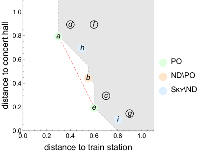
(b)

Figure 1: A set $r$ of locations and their distances to given points of interest.

Example 1

Consider the dataset $r$ in Figure LABEL:fig:example-table, showing locations with their distance from points of interest. The non-dominated options in $r$ are a, b, h, e, i: this is ${\textsc{Sky}}(r)$. Consider now the set $\mathcal{F}$ to be the scoring functions of the form $f(x,y)=w_{1}x+w_{2}y$, where $w_{1}>w_{2}$, i.e., linearly combining distances, with more importance given to the train station. Under $\mathcal{F}$, h and i are $\mathcal{F}$-dominated by a and e, respectively, so only a, b and e are in ${\textsc{ND}}(r;\mathcal{F})$. The gray area in Figure 1b represents the union of $\mathcal{F}$-dominance regions ${\textsc{DR}}(\texttt{a};\mathcal{F})\cup{\textsc{DR}}(\texttt{b};\mathcal{F})\cup{\textsc{DR}}(\texttt{e};\mathcal{F})$. Finally, b can never be top-$1$, since no linear combination of its scores can make it better than a or e; so, ${\textsc{PO}}(r;\mathcal{F})$ consists of just a and e.

Among the ways to test $\mathcal{F}$-dominance when $\mathcal{F}$ is a set of functions under a set of linear constraints $\mathcal{C}$ on the weights, the most efficient one consists in determining the $\mathcal{F}$-dominance region of the candidate $\mathcal{F}$-dominant tuple and checking whether the other tuple belongs to it. This approach, described in Theorem 4.2 in [18], requires enumerating the vertices of the convex polytope defined by $\mathcal{C}$. We will then consider the implementation denoted SVE1F [18], which uses vertex enumeration and also exploits pre-sorting of the dataset (as in SFS [10]). Additionally, SVE1F is a one-phase algorithm, in that it computes its result directly from $r$ instead of first computing ${\textsc{Sky}}(r)$ (which would be possible, since ${\textsc{ND}}(r;\mathcal{F})={\textsc{ND}}({\textsc{Sky}}(r);\mathcal{F})$) – an approach that has been recognized to be more efficient if the constraints are tight enough.

Computing PO can also be done through an LP problem. Testing whether $t\in{\textsc{PO}}$ requires solving an expensive LP problem involving all the tuples. An incremental approach is, however, possible: smaller LP problems with only a part of the tuples may be used to discard tuples. With this, we can solve LP problems of increasing sizes, starting from just two tuples, and then doubling such a number at each round, until all tuples are included. We will adopt the implementation known as POPI2[18], which is incremental and works in two phases, i.e., computes its result from ${\textsc{ND}}(r;\mathcal{F})$ instead of $r$, observing that ${\textsc{PO}}(r;\mathcal{F})={\textsc{PO}}({\textsc{ND}}(r;\mathcal{F});\mathcal{F})$ and that for PO this is much more efficient than a single phase.

3 Parallel computation of flexible skylines

A general scheme for parallelizing the computation of flexible skylines is based on the idea that the dataset can be partitioned and each partition is processed independently and in parallel. This produces a “local” result; the union of all local results still has some redundancies that can be eliminated by applying a last (sequential) round of removal. This approach has been described for skylines, e.g., in [20], and is correct, since, when $r=r_{1}\cup\ldots\cup r_{p}$, with $r_{i}\cap r_{j}=\emptyset$ for $i\neq j$, we have ${\textsc{Sky}}(r)={\textsc{Sky}}({\textsc{Sky}}(r_{1})\cup\ldots\cup{\textsc{Sky}}(r_{p}))$. A similar principle applies to $\mathcal{F}$-skylines by replacing in the above formula ${\textsc{Sky}}(\cdot)$ with ${\textsc{ND}}(\cdot;\mathcal{F})$ or ${\textsc{PO}}(\cdot;\mathcal{F})$.

1. relation $r$, functions $\mathcal{F}$ via constraints $\mathcal{C}$, number of partitions $p$

2. a flexible skyline ${\textsc{ND}}(r;\mathcal{F})$ or ${\textsc{PO}}(r;\mathcal{F})$

3. $ls:=\emptyset$ // the local result

4. $(r_{1},\ldots,r_{p},meta):=\texttt{Partition}(r,p)$ // partitions and meta-information

5. parallel for each $r_{i}$ in $r_{1},\ldots,r_{p}$ do

6. $ls:=ls\cup\texttt{ComputeLocalSet}(r_{i},meta)$

7. return ${\textsc{ND}}(ls;\mathcal{F})$ or ${\textsc{PO}}(ls;\mathcal{F})$

Algorithm 1 Algorithmic pattern for parallel skyline computation.

The algorithmic pattern in Algorithm 1 does this in three phases: first $r$ is partitioned into $r_{1},\ldots,r_{p}$ (line 2), with possible meta-information to be used later; then, (local) results are computed independently (line 3) and in parallel, possibly using the meta-information; finally, all the local results are merged (line 4) and processed sequentially (line 5).

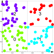
(a)

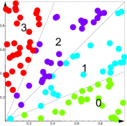
(b)

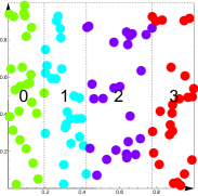
(c)

Figure 2: Partitioning Strategies.

We shall adopt for flexible skylines the same partitioning strategies used in the literature for computing skylines, which are summarized next: Grid Partitioning, Angular Partitioning and Sliced Partitioning. We refrain from considering Random Partitioning [22], which simply randomly distributes the tuples across the various partitions, and is therefore too simple a baseline to receive further attention.

3.1 Partitioning Strategies

3.1.1 Grid Space Partitioning

Grid Partitioning [59] (Grid) divides the space into a grid of equally sized cells. Each dimension is divided into $m$ parts, resulting in a total of $p=m^{d}$ partitions, where $d$ denotes the total number of dimensions. We can also leverage dominance between grid cells to avoid processing certain partitions completely (Grid Filtering). In particular, let $c_{i}.\min$ and $c_{i}.\max$ represent the corners of cell $c_{i}$ with the lowest (best) or respectively highest (worst) values on all dimensions. If $c_{i}.\max$ dominates $c_{j}.\min$ then all tuples in $c_{i}$ dominate all tuples in $c_{j}$, so if $c_{i}$ contains some tuple, $c_{j}$ can be disregarded.

With values in $[0,1]$, the partition for a tuple $t$ can be computed as follows:

$$p(t)=\sum_{i=1}^{d}\lfloor t[A_{i}]\cdot m\rfloor\cdot m^{i-1}$$

where $A_{i}$ is the $i$-th attribute and $m$ are the slices per dimension. Figure 2a shows $m=2$ partitions per dimension, with a total of $4$ partitions (grid cells).

3.1.2 Angle-based Space Partitioning

Angle-based Partitioning [70] (Angular) partitions the space based on angular coordinates, after converting Cartesian to hyper-spherical coordinates. Unlike Grid, Angular does not support any kind of grid dominance.

The partition of tuple $t$ is computed based on hyper-spherical coordinates, including a radial coordinate $r$ and $d-1$ angular coordinates $\varphi_{1},\ldots,\varphi_{d-1}$:

$$p(t)=\sum_{i=1}^{d-1}\left\lfloor\frac{2\varphi_{i}}{\pi}m\right\rfloor m^{i-1}$$ (3)

where $m$ is, again, the number of slices in which each (angular) dimension is divided, which amounts to grid partitioning on angular coordinates. Figure 2b shows Angular at work.

3.1.3 Sliced Partitioning (One-dimensional Slicing)

Sliced Partitioning (Sliced) sorts the dataset on one dimension. The $i$-th tuple $t$ in the ordering is assigned to a partition in the following way:

$$p(t)=\left\lfloor\frac{(i-1)\cdot p}{N-1}\right\rfloor,$$

where $N$ is the number of tuples and $p$ the number of partitions. Figure 2c shows the effect of Sliced.

3.2 Improvements

A number of improvements are possible on top of the previously described algorithmic pattern. The first one regards the choice of a selected set of tuples with a high potential for $\mathcal{F}$-dominating other tuples, which might be shared across all partitions from the start. The second improvement consists in trying to eliminate the final sequential pass, which is typically the most time consuming.

3.2.1 Representative Filtering

A set of potentially “strong” tuples (the representatives) from the entire dataset can be selected before entering the parallel phase. These are shared as meta-information across all partitions, so that any tuple dominated by a representative can be deleted with no further ado. A simple selection criterion consists in selecting the first few tuples in each partition after sorting: by virtue of the topological sort property, they cannot be $\mathcal{F}$-dominated by subsequent tuples and therefore are likely to $\mathcal{F}$-dominate many of them.

3.2.2 Elimination of sequential phase

A way to eliminate the final sequential phase is, instead of computing the global set sequentially from the union $U$ of the local sets, to re-partition $U$ into $u_{1},\ldots,u_{p}$ for a new parallel phase and also pass to each partition the entire $U$ as meta-information. With this, we can eliminate from each partition $u_{i}$ the (globally) $\mathcal{F}$-dominated tuples (i.e., those that are dominated by some tuple in $U$). We call this scheme NoSeq.

4 Experiments

In this section, we measure the efficiency of the proposed algorithmic pattern for the computation of both ND and PO. We measure our indicators of efficiency in different settings according to the operating parameters described in Table 1. In particular, we target anticorrelated datasets, which are the most challenging in any skyline-like scenario. The set $\mathcal{F}$ of functions considered for computing flexible skylines is simply characterized by the constraint $w_{1}\geq w_{2}$, which prunes 50% of the space of weights and can be applied to any dataset with at least $d\geq 2$ dimensions.

Our experiments are conducted on a computational infrastructure with Spark comprising virtual machines equipped with a total of 30 cores and 8GB of RAM.

Table 1: Operating parameters for testing efficiency (defaults in bold).

Full name	Tested value
Dataset size ($N$)	200K, 500K, 1M, 2M, 5M, 10M
# of dimensions ($d$)	2, 4, 6, 7
# of partitions ($p$)	10, 50, 100, 150, 200, 300
# of cores ($c$)	5, 10, 20, 30

Varying the dataset size. Our first experiments test how efficiency varies as we vary the dataset size $N$ and keep all other parameters set to a default value, i.e., $d=4$ dimensions, $p=100$ partitions, and $c=30$ cores.

Figure 3a shows that, while of course execution times grow as the size grows, the Sliced strategy is much more efficient than Angular and, especially, Grid in exploiting parallelism during the computation of ND with SVE1F. In particular, Figure 3b shows the time spent during the parallel phase, highlighting how Grid goes astray and is inefficient in that many partitions are unbalanced, while the other two partitioning strategies are much more balanced in this respect. Finally, Figure 4 shows the percentage of tuples that are removed during the parallel phase, highlighting again that Grid is the least efficient choice, while Angular has the highest trimming power, although it is overall less efficient than Sliced because it pays an overhead due to the partial imbalance between partitions (which are perfectly balanced in case of Sliced).

Table 2 shows the breakdown of the execution times between the parallel and the sequential phase, along with the number of tuples surviving after the parallel phase, for a 4d dataset with 2M tuples, confirming the highest benefits of the Sliced strategy.

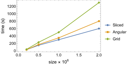
(a)

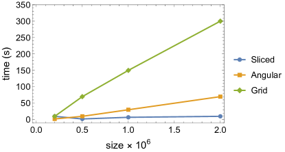
(b)

Figure 3: Performance of SVE1F on an anticorrelated dataset with $d=4$ dimensions and varying sizes: total execution times (a); time for the parallel phase (b).

.

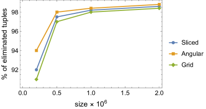
Figure 4: Percentage of removed tuples during the parallel phase by SVE1F on an anticorrelated dataset with $d=4$ dimensions and varying sizes.

Table 2: Time of parallel and sequential phases with the SVE1F Algorithm using a 4d anticorrelated dataset with 2 million points and 16781 ND points.

Partitioning	$|\bigcup{\textsc{ND}}_{i}|$	parallel phase ($s$)	sequential phase ($s$)
Grid	39946	325.6	970.0
Angular	33971	68.3	776.9
Sliced	28051	14.8	679.3

We perform a similar analysis with PO using POPI2. We do not include results regarding Grid here, because, for solving LP problems of this size, we need partitions to be as balanced as possible, while Grid produces extremely unbalanced partitions (especially with anticorrelated data), with consequently very poor results. Figure 5a shows the times required to compute PO from ND by using POPI2 (the time to compute ND is thus not included in the total). We observe that, in this case, Sliced performs much more poorly than Angular, and this although Sliced still incurs lower execution times during the parallel phase, as shown in Figure 5b. The reason is that the partitioning along one single dimension effected by Sliced is not particularly efficient at removing tuples during the parallel phase, as Figure 6 shows, with Angular removing as many as 85% of the tuples with a 4d anticorrelated dataset with 2M tuples, while Sliced only attains 62% in that case. To be precise, PO is a very small set compared to ND (with $|{\textsc{ND}}|=16,781$ and $|{\textsc{PO}}|=150$ with the 4d dataset of 2M tuples), and this might be the source of ineffectiveness of sorting the dataset in one dimension as in Sliced. Table 3 shows the execution times of the parallel and the sequential phase for a 4d dataset with 2 million tuples, highlighting that the Sliced strategy incurs a very high overhead in the sequential phase, due to a much worse ability to remove tuples during the parallel phase, with more than three times as many tuples remaining with the Sliced strategy than with the Angular strategy.

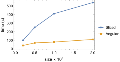
(a)

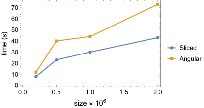
(b)

Figure 5: Performance of POPI2 on an anticorrelated dataset with $d=4$ dimensions and varying sizes: total execution times (a); time for the parallel phase (b).

.

Table 3: Time of parallel and sequential phases with the POPI2 Algorithm using a 4d anticorrelated dataset with 2 million points and 16781 ND points and 150 PO points.

Partitioning	$|\bigcup{\textsc{PO}}_{i}|$	parallel phase ($s$)	sequential phase ($s$)
Angular	1544	72.4	48.9
Sliced	5108	46.5	504.5

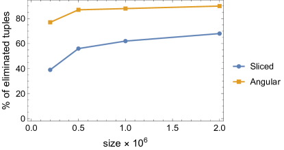
Figure 6: Percentage of removed tuples during the parallel phase by POPI2 on an anticorrelated dataset with $d=4$ dimensions and varying sizes.

.

Varying size: improved strategies. Figure 7 shows the effect of applying the improvements discussed in Section 3.2. Representative Filtering causes slight improvements in terms of execution times with both Sliced and Angular, as can be seen in Figure 7a for the computation of ND, where the improved versions are indicated as Sliced+ and Angular+. We also applied the NoSeq scheme on top of the Sliced partitioning strategy (with representatives), which has determined significant improvements in the computation of ND. It turns out that NoSeq largely outperforms the other strategies, with overall execution times that are more than 7 times smaller than the second best strategy (Sliced+). Grid Filtering, available for Grid partitioning, takes too long to return the local set and is overall disadvantageous in terms of duration compared to the basic version, so we will not consider it in the experiments.

As for the computation of PO with POPI2, Figure 7b reports the NoSeq strategy along with Sliced and Angular (representatives prove to be ineffective for computing PO and thus not reported). We observe that applying the NoSeq scheme on top of Sliced makes it even more efficient than Angular, which was be the best option for this kind of problem.

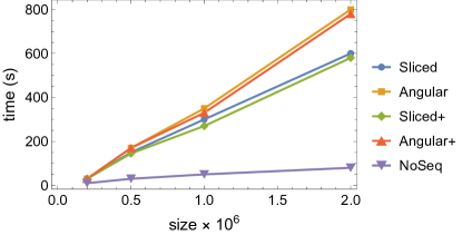
(a)

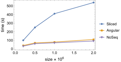
(b)

Figure 7: Performance of improved variants on an anticorrelated dataset with $d=4$ dimensions and varying sizes: total execution times for SVE1F (a) and POPI2 (b).

.

In order to complete our analysis as the size varies, we also tested the behavior of the NoSeq strategy with even larger dataset sizes. Figure 8 shows that, from 1M to 10M tuples, execution times incurred with NoSeq follow an almost perfectly linear growth with the dataset size, both for ND and for PO, confirming scalability of the approach.

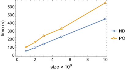
Figure 8: Performance of the NoSeq strategy on an anticorrelated dataset with $d=4$ dimensions and varying sizes: total execution times for SVE1F and POPI2.

.

Varying dimensions. Increasing the number of dimensions $d$ results in a notable rise in execution time due to the significantly larger number of tuples in the output. As the number of dimensions increases, the probability of a tuple being $\mathcal{F}$-dominated decreases substantially. Figure 9 illustrates that, for anticorrelated datasets, NoSeq is also affected by the “curse of dimensionality”, with execution times increasing at a rate greater than linear as the number of dimensions grows.

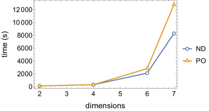
Figure 9: Performance of the NoSeq strategy on an anticorrelated dataset with size $N=$1M and varying dimensions: total execution times for SVE1F and POPI2.

.

Varying number of partitions. The lowest execution times are reached when the number of partitions $p$ is a small multiple of the number of available cores (30). For larger values of $p$, there is an increase in execution time due to synchronization overhead between nodes. Figure 10 shows this for several values of $p$, with the extra observation that, while for Sliced (and NoSeq, which is built on top of Sliced+) all values of $p$ are possible, Angular and Grid are constrained to have a number of partitions that equals $m^{d}$ and $m^{d-1}$, respectively, where $m$ is the number of slices per dimension. The best value for $p$ is around 150 (i.e., five times the number of available cores), after which performances start degrading. The NoSeq strategy consistently outperforms the others for the computation of ND.

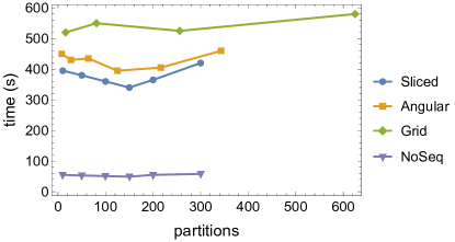
Figure 10: Performance of various strategies for computing ND on a 4d anticorrelated dataset with size $N=$1M and varying partitions.

.

Varying number of cores. In our last experiment, we assess the effect of the number of cores $c$ on the execution time. Figure 11 shows benefits from the increased availability of cores, with the most visible effects near the beginning of the increase, when doubling the number of cores from 5 to 10. Adding further resources keeps improving execution times, but with more moderate benefits. Overall, the NoSeq strategy manages to improve its execution time by three times for computing ND and by $3.4$ times for computing PO when moving from 5 to 30 cores.

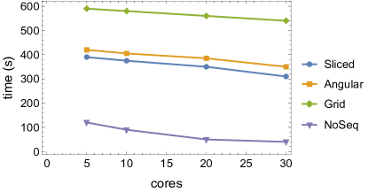
(a)

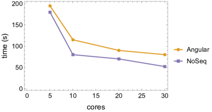
(b)

Figure 11: Effect of the number of cores $c$ on the execution time incurred by SVE1F (a) and POPI2 (b) on an anticorrelated dataset with $d=4$ dimensions and size $N=$1M.

.

5 Related Work

There is an abundant literature that has studied and proposed sequential algorithms for the computation of the skyline, including Block-Nested Loop (BNL) and Divide-and-Conquer [3], Sort Filter Skyline (SFS) [10], Bitmap [68], Branch-and-Bound [61, 62], and Sort and Limit Skyline algorithm (SaLSa) [1]. The pre-sorting imposed by SFS is a suitable strategy for exploiting the topological sort property of dominance, which extends to $\mathcal{F}$-dominance, and has therefore been exploited in the sequential algorithms for computing flexible skylines [18, 14, 16, 15, 2, 17, 57]), including SVE1F and POPI2, which we used here.

Systematic approaches for parallelizing the computation of skylines have been attempted for both vertical partitioning (essentially following Fagin’s middleware scenario for top-k queries [31, 69, 9]) and horizontal partitioning [24], which we considered in the present work. Horizontal partitioning strategies for computing the skyline have found their way to practical implementations with the advent of computation paradigms such as Map-Reduce and Spark, which allow seamless data distribution and processing through Mappers and Reducers, as demonstrated in [64, 25, 63, 20], together with optimization opportunities given by representative tuples and the elimination of the final sequential round, which was partially advocated in [59].

While other works have considered flexible skylines in the context of vertical distribution [16, 46], the case of horizontal partitioning is, to the best of our knowledge, novel.

While classical skylines have no support for preferences, top-$k$ queries are the alternative (and, typically, preferred) ranking tool that not only supports preferences through scoring functions, but also controls the output size and accommodates various kinds of queries [41, 50, 51]. Many attempts are known that have tried to amalgamate top-$k$ queries and skylines so as to get the most out of these tools [14, 57].

Partitioning schemes similar to those that we have used in this paper have been successfully employed also for the computation of indicators of strength of skyline tuples, i.e., numeric values that can be adopted for endowing skyline tuples with further attributes to be used for ranking purposes. These indicators include, e.g., the count of dominated tuples [61], the stability to perturbations in the scoring functions [67], and the best possible rank of a tuple when using a linear scoring function [58]. Several other indicators are introduced in [19], some requiring to build the convex hull of a dataset [60, 71, 42], or to compute complex volumes [40, 5]; one of these indicators, called grid resistance, can be computed through parallel partitioning schemes similar to those discussed in this paper [47, 48],

Skylines, and more so flexible skylines, are common components of complex data preparation pipelines, typically followed by Machine Learning or Clustering algorithms [52, 54, 55, 56] applied to data that might be collected by heterogeneous sources like RFID [33, 32], pattern mining [53], crowdsourcing applications [34, 4, 43], and streaming data [23]. In particular, the role of (flexible) skylines and top-$k$ queries is orthogonal to and typically integrated with that of query optimization and query explanation, which may rely on semantic properties of data expressible, e.g., through Query Containment (QC) [8, 66, 7, 6] and integrity constraints [45, 12, 13, 44, 65, 49, 11].

While the preferences expressible with scoring functions and constraints on weights are of a quantitative nature, it would be interesting to know the extent to which qualitative preferences [21] could also be integrated in the flexible skyline framework.

Other possible research avenues regard the stability of the results of a flexible skyline in the face of inconsistent or missing values [27, 26, 28, 29], rather than uncertainty in the scoring function, and how this depends on the amount of such an inconsistency in the data [35, 30, 36, 37, 38, 39].

6 Conclusion

In this paper, we tackled the problem of computing flexible skylines by exploiting common partitioning schemes that divide a dataset horizontally and send each partition to a different compute node for an initial round of computation of the result. The partial results, after this parallel phase, are collected and ultimately processed for a final, sequential round that eliminates all redundancies. While this consolidated scheme has been successfully used for computing the classical skyline operator, ours is the first attempt to apply it to the case of flexible skylines — an extension of skylines that accommodates user preferences expressed through constraints on weights.

Our results show that the partitioning is generally beneficial, especially with schemes that divide the dataset into more balanced subsets, such as Angular and Sliced. In addition to optimization opportunities based on the notion of representative tuples, we also adopted another optimization, indicated as NoSeq, that removes the final sequential round completely, which is typically the most expensive part of the entire computation. Indeed, NoSeq proves to be the most robust of all tested algorithmic solutions.

The computation of the two flexible skyline operators, ND and PO, differs in the ability of the partitioning strategy to effectively reduce the set of candidates before the final round. We noticed that, while Sliced does its job egregiously in the case of ND, the smaller sizes involved in the computation of potentially optimal tuples make Sliced a less suitable candidate than Angular for PO. In both cases, however, the NoSeq strategy proves to be the best option.

Future research might try to address the impact of the constraints on weights on the effectiveness of the partitioning strategy.

References

- [1] I. Bartolini, P. Ciaccia, and M. Patella. Salsa: computing the skyline without scanning the whole sky. In P. S. Yu, V. J. Tsotras, E. A. Fox, and B. Liu, editors, Proceedings of the 2006 ACM CIKM International Conference on Information and Knowledge Management, Arlington, Virginia, USA, November 6-11, 2006, pages 405–414. ACM, 2006.
- [2] M. V. N. Bedo, P. Ciaccia, D. Martinenghi, and D. de Oliveira. A k-skyband approach for feature selection. In G. Amato, C. Gennaro, V. Oria, and M. Radovanovic, editors, Similarity Search and Applications - 12th International Conference, SISAP 2019, Newark, NJ, USA, October 2-4, 2019, Proceedings, volume 11807 of Lecture Notes in Computer Science, pages 160–168. Springer, 2019.
- [3] S. Börzsönyi, D. Kossmann, and K. Stocker. The skyline operator. In Proceedings of the 17th International Conference on Data Engineering, April 2-6, 2001, Heidelberg, Germany, pages 421–430, 2001.
- [4] A. Bozzon, I. Catallo, E. Ciceri, P. Fraternali, D. Martinenghi, and M. Tagliasacchi. A framework for crowdsourced multimedia processing and querying. In Proceedings of the First International Workshop on Crowdsourcing Web Search, Lyon, France, April 17, 2012, pages 42–47, 2012.
- [5] K. Bringmann and T. Friedrich. Approximating the least hypervolume contributor: Np-hard in general, but fast in practice. Theor. Comput. Sci., 425:104–116, 2012.
- [6] A. Calì, D. Calvanese, and D. Martinenghi. Dynamic Query Optimization under Access Limitations and Dependencies. Journal of Universal Computer Science, 15(21):33–62, 2009. (SJR: Q2).
- [7] A. Calì and D. Martinenghi. Conjunctive query containment under access limitations. In Q. Li, S. Spaccapietra, E. S. K. Yu, and A. Olivé, editors, Conceptual Modeling - ER 2008, 27th International Conference on Conceptual Modeling, Barcelona, Spain, October 20-24, 2008. Proceedings, volume 5231 of Lecture Notes in Computer Science, pages 326–340. Springer, 2008.
- [8] A. K. Chandra and P. M. Merlin. Optimal implementation of conjunctive queries in relational databases. In Proceedings of the 9th Annual ACM Symposium on Theory of Computing, pages 77–90. ACM, 1977.
- [9] J. Chomicki, P. Ciaccia, and N. Meneghetti. Skyline queries, front and back. SIGMOD Record, 42(3):6–18, 2013.
- [10] J. Chomicki, P. Godfrey, J. Gryz, and D. Liang. Skyline with presorting. In U. Dayal, K. Ramamritham, and T. M. Vijayaraman, editors, Proceedings of the 19th International Conference on Data Engineering, March 5-8, 2003, Bangalore, India, pages 717–719. IEEE Computer Society, 2003.
- [11] H. Christiansen and D. Martinenghi. Symbolic constraints for meta-logic programming. Appl. Artif. Intell., 14(4):345–367, 2000.
- [12] H. Christiansen and D. Martinenghi. Simplification of database integrity constraints revisited: A transformational approach. In M. Bruynooghe, editor, Logic Based Program Synthesis and Transformation, 13th International Symposium LOPSTR 2003, Uppsala, Sweden, August 25-27, 2003, Revised Selected Papers, volume 3018 of Lecture Notes in Computer Science, pages 178–197. Springer, 2003.
- [13] H. Christiansen and D. Martinenghi. Simplification of integrity constraints for data integration. In D. Seipel and J. M. T. Torres, editors, Foundations of Information and Knowledge Systems, Third International Symposium, FoIKS 2004, Wilhelminenberg Castle, Austria, February 17-20, 2004, Proceedings, volume 2942 of Lecture Notes in Computer Science, pages 31–48. Springer, 2004.
- [14] P. Ciaccia and D. Martinenghi. Reconciling skyline and ranking queries. PVLDB, 10(11):1454–1465, 2017.
- [15] P. Ciaccia and D. Martinenghi. Beyond skyline and ranking queries: Restricted skylines (extended abstract). In S. Bergamaschi, T. D. Noia, and A. Maurino, editors, Proceedings of the 26th Italian Symposium on Advanced Database Systems, Castellaneta Marina (Taranto), Italy, June 24-27, 2018, volume 2161 of CEUR Workshop Proceedings. CEUR-WS.org, 2018.
- [16] P. Ciaccia and D. Martinenghi. FA + TA < FSA: Flexible score aggregation. In Proceedings of the 27th ACM International Conference on Information and Knowledge Management, CIKM 2018, Torino, Italy, October 22-26, 2018, pages 57–66, 2018.
- [17] P. Ciaccia and D. Martinenghi. Flexible score aggregation (extended abstract). In M. Mecella, G. Amato, and C. Gennaro, editors, Proceedings of the 27th Italian Symposium on Advanced Database Systems, Castiglione della Pescaia (Grosseto), Italy, June 16-19, 2019, volume 2400 of CEUR Workshop Proceedings. CEUR-WS.org, 2019.
- [18] P. Ciaccia and D. Martinenghi. Flexible skylines: Dominance for arbitrary sets of monotone functions. ACM Trans. Database Syst., 45(4):18:1–18:45, 2020.
- [19] P. Ciaccia and D. Martinenghi. Directional Queries: Making Top-k Queries More Effective in Discovering Relevant Results. Proc. ACM Manag. Data, 2(6), 2024. (GGS: A++).
- [20] P. Ciaccia and D. Martinenghi. Optimization strategies for parallel computation of skylines. CoRR, arxiv:2411.14968, 2024.
- [21] P. Ciaccia, D. Martinenghi, and R. Torlone. Foundations of context-aware preference propagation. J. ACM, 67(1):4:1–4:43, 2020.
- [22] A. Cosgaya-Lozano, A. Rau-Chaplin, and N. Zeh. Parallel computation of skyline queries. In 21st Annual International Symposium on High Performance Computing Systems and Applications (HPCS 2007), 13-16 May 2007, Saskatoon, Saskatchewan, Canada, page 12. IEEE Computer Society, 2007.
- [23] G. Costa, G. Manco, and E. Masciari. Dealing with trajectory streams by clustering and mathematical transforms. J. Intell. Inf. Syst., 42(1):155–177, 2014.
- [24] B. Cui, L. Chen, L. Xu, H. Lu, G. Song, and Q. Xu. Efficient skyline computation in structured peer-to-peer systems. IEEE Trans. Knowl. Data Eng., 21(7):1059–1072, 2009.
- [25] E. De Lorenzis. Computation of flexible skylines in a distributed environment, 2022. Master’s Thesis, Politecnico di Milano.
- [26] H. Decker and D. Martinenghi. Avenues to flexible data integrity checking. In 17th International Workshop on Database and Expert Systems Applications (DEXA 2006), 4-8 September 2006, Krakow, Poland, pages 425–429. IEEE Computer Society, 2006.
- [27] H. Decker and D. Martinenghi. A relaxed approach to integrity and inconsistency in databases. In M. Hermann and A. Voronkov, editors, Logic for Programming, Artificial Intelligence, and Reasoning, 13th International Conference, LPAR 2006, Phnom Penh, Cambodia, November 13-17, 2006, Proceedings, volume 4246 of Lecture Notes in Computer Science, pages 287–301. Springer, 2006.
- [28] H. Decker and D. Martinenghi. Getting rid of straitjackets for flexible integrity checking. In 18th International Workshop on Database and Expert Systems Applications (DEXA 2007), 3-7 September 2007, Regensburg, Germany, pages 360–364. IEEE Computer Society, 2007.
- [29] H. Decker and D. Martinenghi. Classifying integrity checking methods with regard to inconsistency tolerance. In S. Antoy and E. Albert, editors, Proceedings of the 10th International ACM SIGPLAN Conference on Principles and Practice of Declarative Programming, July 15-17, 2008, Valencia, Spain, pages 195–204. ACM, 2008.
- [30] H. Decker and D. Martinenghi. Modeling, measuring and monitoring the quality of information. In C. A. Heuser and G. Pernul, editors, Advances in Conceptual Modeling - Challenging Perspectives, ER 2009 Workshops CoMoL, ETheCoM, FP-UML, MOST-ONISW, QoIS, RIGiM, SeCoGIS, Gramado, Brazil, November 9-12, 2009. Proceedings, volume 5833 of Lecture Notes in Computer Science, pages 212–221. Springer, 2009.
- [31] R. Fagin. Fuzzy queries in multimedia database systems. In A. O. Mendelzon and J. Paredaens, editors, Proceedings of the Seventeenth ACM SIGACT-SIGMOD-SIGART Symposium on Principles of Database Systems, June 1-3, 1998, Seattle, Washington, USA, pages 1–10, 1998.
- [32] B. Fazzinga, S. Flesca, F. Furfaro, and E. Masciari. Rfid-data compression for supporting aggregate queries. ACM Trans. Database Syst., 38(2):11, 2013.
- [33] B. Fazzinga, S. Flesca, E. Masciari, and F. Furfaro. Efficient and effective RFID data warehousing. In B. C. Desai, D. Saccà, and S. Greco, editors, International Database Engineering and Applications Symposium (IDEAS 2009), September 16-18, 2009, Cetraro, Calabria, Italy, ACM International Conference Proceeding Series, pages 251–258, 2009.
- [34] L. Galli, P. Fraternali, D. Martinenghi, M. Tagliasacchi, and J. Novak. A draw-and-guess game to segment images. In 2012 International Conference on Privacy, Security, Risk and Trust, PASSAT 2012, and 2012 International Conference on Social Computing, SocialCom 2012, Amsterdam, Netherlands, September 3-5, 2012, pages 914–917, 2012.
- [35] J. Grant and A. Hunter. Measuring inconsistency in knowledgebases. J. Intell. Inf. Syst., 27(2):159–184, 2006.
- [36] J. Grant and A. Hunter. Measuring the good and the bad in inconsistent information. In T. Walsh, editor, IJCAI 2011, Proceedings of the 22nd International Joint Conference on Artificial Intelligence, Barcelona, Catalonia, Spain, July 16-22, 2011, pages 2632–2637. IJCAI/AAAI, 2011.
- [37] J. Grant and A. Hunter. Distance-based measures of inconsistency. In L. C. van der Gaag, editor, Symbolic and Quantitative Approaches to Reasoning with Uncertainty - 12th European Conference, ECSQARU 2013, Utrecht, The Netherlands, July 8-10, 2013. Proceedings, volume 7958 of Lecture Notes in Computer Science, pages 230–241. Springer, 2013.
- [38] J. Grant and A. Hunter. Analysing inconsistent information using distance-based measures. Int. J. Approx. Reason., 89:3–26, 2017.
- [39] J. Grant and A. Hunter. Semantic inconsistency measures using 3-valued logics. Int. J. Approx. Reason., 156:38–60, 2023.
- [40] A. P. Guerreiro, C. M. Fonseca, and L. Paquete. The hypervolume indicator: Computational problems and algorithms. ACM Comput. Surv., 54(6):119:1–119:42, 2022.
- [41] I. F. Ilyas, G. Beskales, and M. A. Soliman. A survey of top-k query processing techniques in relational database systems. ACM Comput. Surv., 40(4), 2008.
- [42] H. Kwon, S. Oh, and J.-W. Baek. Algorithmic efficiency in convex hull computation: Insights from 2d and 3d implementations. Symmetry, 16(12), 2024.
- [43] B. Loni, M. Menendez, M. Georgescu, L. Galli, C. Massari, I. S. Altingövde, D. Martinenghi, M. Melenhorst, R. Vliegendhart, and M. Larson. Fashion-focused creative commons social dataset. In Multimedia Systems Conference 2013, MMSys ’13, Oslo, Norway, February 27 - March 01, 2013, pages 72–77, 2013. (GGS: B-).
- [44] D. Martinenghi. Simplification of integrity constraints with aggregates and arithmetic built-ins. In H. Christiansen, M. Hacid, T. Andreasen, and H. L. Larsen, editors, Flexible Query Answering Systems, 6th International Conference, FQAS 2004, Lyon, France, June 24-26, 2004, Proceedings, volume 3055 of Lecture Notes in Computer Science, pages 348–361. Springer, 2004.
- [45] D. Martinenghi. Advanced Techniques for Efficient Data Integrity Checking. PhD thesis, Roskilde University, Dept. of Computer Science, Roskilde, Denmark, 2005. Available in Datalogiske Skrifter, vol. 105, Roskilde University, Denmark.
- [46] D. Martinenghi. Computing the non-dominated flexible skyline in vertically distributed datasets with no random access. CoRR, arXiv:2412.15468, 2024.
- [47] D. Martinenghi. Parallelizing the computation of robustness for measuring the strength of tuples. CoRR, arXiv:2412.02274, 2024.
- [48] D. Martinenghi. Parallelizing the Computation of Grid Resistance to Measure the Strength of Skyline Tuples. Algorithms, 18(1), 2025.
- [49] D. Martinenghi and H. Christiansen. Transaction management with integrity checking. In K. V. Andersen, J. K. Debenham, and R. R. Wagner, editors, Database and Expert Systems Applications, 16th International Conference, DEXA 2005, Copenhagen, Denmark, August 22-26, 2005, Proceedings, volume 3588 of Lecture Notes in Computer Science, pages 606–615. Springer, 2005.
- [50] D. Martinenghi and M. Tagliasacchi. Proximity rank join. Proc. VLDB Endow., 3(1):352–363, 2010.
- [51] D. Martinenghi and M. Tagliasacchi. Cost-aware rank join with random and sorted access. IEEE Trans. Knowl. Data Eng., 24(12):2143–2155, 2012.
- [52] E. Masciari. Trajectory clustering via effective partitioning. In T. Andreasen, R. R. Yager, H. Bulskov, H. Christiansen, and H. L. Larsen, editors, Flexible Query Answering Systems, 8th International Conference, FQAS 2009, Roskilde, Denmark, October 26-28, 2009. Proceedings, volume 5822 of Lecture Notes in Computer Science, pages 358–370, 2009.
- [53] E. Masciari, S. Gao, and C. Zaniolo. Sequential pattern mining from trajectory data. In B. C. Desai, J. L. Larriba-Pey, and J. Bernardino, editors, 17th International Database Engineering & Applications Symposium, IDEAS ’13, Barcelona, Spain - October 09 - 11, 2013, pages 162–167. ACM, 2013.
- [54] E. Masciari, G. M. Mazzeo, and C. Zaniolo. Analysing microarray expression data through effective clustering. Inf. Sci., 262:32–45, 2014.
- [55] E. Masciari, V. Moscato, A. Picariello, and G. Sperlì. A deep learning approach to fake news detection. In D. Helic, G. Leitner, M. Stettinger, A. Felfernig, and Z. W. Ras, editors, Foundations of Intelligent Systems - 25th International Symposium, ISMIS 2020, Graz, Austria, September 23-25, 2020, Proceedings, volume 12117 of Lecture Notes in Computer Science, pages 113–122. Springer, 2020.
- [56] E. Masciari, V. Moscato, A. Picariello, and G. Sperlì. Detecting fake news by image analysis. In B. C. Desai and W. Cho, editors, IDEAS 2020: 24th International Database Engineering & Applications Symposium, Seoul, Republic of Korea, August 12-14, 2020, pages 27:1–27:5. ACM, 2020.
- [57] K. Mouratidis, K. Li, and B. Tang. Marrying top-k with skyline queries: Relaxing the preference input while producing output of controllable size. In G. Li, Z. Li, S. Idreos, and D. Srivastava, editors, SIGMOD ’21: International Conference on Management of Data, Virtual Event, China, June 20-25, 2021, pages 1317–1330. ACM, 2021.
- [58] K. Mouratidis, J. Zhang, and H. Pang. Maximum rank query. PVLDB, 8(12):1554–1565, 2015.
- [59] K. Mullesgaard, J. L. Pederseny, H. Lu, and Y. Zhou. Efficient skyline computation in mapreduce. In S. Amer-Yahia, V. Christophides, A. Kementsietsidis, M. N. Garofalakis, S. Idreos, and V. Leroy, editors, Proceedings of the 17th International Conference on Extending Database Technology, EDBT 2014, Athens, Greece, March 24-28, 2014, pages 37–48. OpenProceedings.org, 2014.
- [60] M. Nakagawa, D. Man, Y. Ito, and K. Nakano. A simple parallel convex hulls algorithm for sorted points and the performance evaluation on the multicore processors. In 2009 International Conference on Parallel and Distributed Computing, Applications and Technologies, PDCAT 2009, Higashi Hiroshima, Japan, 8-11 December 2009, pages 506–511, 2009.
- [61] D. Papadias, Y. Tao, G. Fu, and B. Seeger. An optimal and progressive algorithm for skyline queries. In A. Y. Halevy, Z. G. Ives, and A. Doan, editors, Proceedings of the 2003 ACM SIGMOD International Conference on Management of Data, San Diego, California, USA, June 9-12, 2003, pages 467–478. ACM, 2003.
- [62] D. Papadias, Y. Tao, G. Fu, and B. Seeger. Progressive skyline computation in database systems. TODS, 30(1):41–82, 2005.
- [63] E. Pinari. Parallel implementations of the skyline query using pyspark, 2022. Master’s Thesis, Politecnico di Milano.
- [64] A. Pindozzi. Scalable solutions for skyline computation using pyspark: Exploring parallel algorithms, 2023. Master’s Thesis, Politecnico di Milano.
- [65] S. D. Samarin and M. Amini. Integrity checking for aggregate queries. IEEE Access, 9:74068–74084, 2021.
- [66] O. Shmueli. Decidability and expressiveness aspects of logic queries. In Proceedings of the sixth ACM SIGACT-SIGMOD-SIGART symposium on Principles of database systems, pages 237–249. ACM Press, 1987.
- [67] M. A. Soliman, I. F. Ilyas, D. Martinenghi, and M. Tagliasacchi. Ranking with uncertain scoring functions: semantics and sensitivity measures. In Proceedings of the ACM SIGMOD International Conference on Management of Data, SIGMOD 2011, Athens, Greece, June 12-16, 2011, pages 805–816, 2011.
- [68] K. Tan, P. Eng, and B. C. Ooi. Efficient progressive skyline computation. In VLDB 2001, Proceedings of 27th International Conference on Very Large Data Bases, September 11-14, 2001, Roma, Italy, pages 301–310. Morgan Kaufmann, 2001.
- [69] G. Trimponias, I. Bartolini, D. Papadias, and Y. Yang. Skyline processing on distributed vertical decompositions. IEEE Trans. Knowl. Data Eng., 25(4):850–862, 2013.
- [70] A. Vlachou, C. Doulkeridis, and Y. Kotidis. Angle-based space partitioning for efficient parallel skyline computation. In J. T. Wang, editor, Proceedings of the ACM SIGMOD International Conference on Management of Data, SIGMOD 2008, Vancouver, BC, Canada, June 10-12, 2008, pages 227–238. ACM, 2008.
- [71] Y. Wang, R. Yesantharao, S. Yu, L. Dhulipala, Y. Gu, and J. Shun. Pargeo: A library for parallel computational geometry. In S. Chechik, G. Navarro, E. Rotenberg, and G. Herman, editors, 30th Annual European Symposium on Algorithms, ESA 2022, September 5-9, 2022, Berlin/Potsdam, Germany, volume 244 of LIPIcs, pages 88:1–88:19, 2022.