The Geodesic Fréchet Distance Between Two Curves Bounding a Simple Polygon

Abstract

The Fréchet distance is a popular similarity measure that is well-understood for polygonal curves in $\mathbb{R}^{d}$: near-quadratic time algorithms exist, and conditional lower bounds suggest that these results cannot be improved significantly, even in one dimension and when approximating with a factor less than three. We consider the special case where the curves bound a simple polygon and distances are measured via geodesics inside this simple polygon. Here the conditional lower bounds do not apply; Efrat et al. (2002) were able to give a near-linear time $2$-approximation algorithm.

In this paper, we significantly improve upon their result: we present a $(1+\varepsilon)$-approximation algorithm, for any $\varepsilon>0$, that runs in $\mathcal{O}(\frac{1}{\varepsilon}(n+m\log n)\log nm\log\frac{1}{\varepsilon})$ time for a simple polygon bounded by two curves with $n$ and $m$ vertices, respectively. To do so, we show how to compute the reachability of specific groups of points in the free space at once and in near-linear time, by interpreting their free space as one between separated one-dimensional curves. Bringmann and Künnemann (2015) previously solved the decision version of the Fréchet distance in this setting in $\mathcal{O}((n+m)\log nm)$ time. We strengthen their result and compute the Fréchet distance between two separated one-dimensional curves in linear time. Finally, we give a linear time exact algorithm if the two curves bound a convex polygon.

1 Introduction

The Fréchet distance is a well-studied similarity measure for curves in a metric space. Most results so far concern the Fréchet distance between two polygonal curves $R$ and $B$ in $\mathbb{R}^{d}$ with $n$ and $m$ vertices, respectively. The Fréchet distance between two such curves can be computed in $\tilde{\mathcal{O}}(nm)$ time (see e.g. [1, 6]). There is a (nearly) matching conditional lower bound: If the Fréchet distance between polygonal curves can be computed in $\mathcal{O}(n^{2-\varepsilon})$ time for the case $m=n$, then the Strong Exponential Time Hypothesis (SETH) fails [4]. This lower bound holds even in one dimension and for any approximation with a factor less than three [7]. In fact, so far there is no algorithm for general curves that gives any constant-factor approximation in strongly-subquadratic time. We were the first to present an algorithm that results in an arbitrarily small polynomial approximation factor ($n^{\varepsilon}$ for any $\varepsilon\in(0,1]$) in strongly-subquadratic time ($\tilde{\mathcal{O}}(n^{2-\varepsilon})$) [21]. However, the polynomial approximation barrier is yet to be broken in the general case.

For certain families of “realistic” curves, the SETH lower bound does not apply. For example, when the curves are $c$-packed, Bringmann and Künnemann [5] give a $(1+\varepsilon)$-approximation algorithm, for any $\varepsilon>0$, that runs in $\tilde{\mathcal{O}}(cn/\sqrt{\varepsilon})$ time. When the curves are $\kappa$-bounded or $\phi$-low density, for constant $\kappa$ or $\phi$, Driemel et al. [12] give strongly-subquadratic $(1+\varepsilon)$-approximation algorithms as well. Moreover, if the input curves have an imbalanced number of vertices, then the Fréchet distance of one-dimensional curves can be computed in strongly-subquadratic time without making extra assumptions about the shape of the curves. This was recently established by Blank and Driemel [3], who give an $\tilde{\mathcal{O}}(n^{2\alpha}+n)$-time algorithm when $m=n^{\alpha}$ for some $\alpha\in(0,1)$.

In this paper we investigate the Fréchet distance in the presence of obstacles. If the two polygonal curves $R$ and $B$ lie inside a simple polygon $P$ with $k$ vertices and we measure distances by the geodesic distance inside $P$, then neither the upper nor the conditional lower bound change in a fundamental way. Specifically, Cook and Wenk [10] show how to compute the Fréchet distance in this setting in $\mathcal{O}(k+N^{2}\log kN\log N)$ time, with $N=\max\{n,m\}$. For more general polygonal obstacles, Chambers et al. [8] give an algorithm that computes the homotopic Fréchet distance in $\mathcal{O}(N^{9}\log N)$ time, where $N=m+n+k$ is the total number of vertices on the curves and obstacles.

We are investigating the specific setting where the two curves bound a simple region, that is, both $R$ and $B$ are simple, meet only at their first and last endpoints, and lie on the boundary of the region. We measure distance by the geodesic Fréchet distance inside that region. If $R$ and $B$ bound a triangulated topological disk $D$ with $k$ faces, then Har-Peled et al. [18] give an $\mathcal{O}(\log n)$-approximation algorithm that runs in $\mathcal{O}(k^{6}\log k)$ time. If the region is a simple polyon $P$ (see figure) then the SETH lower bound does not apply. Efrat et al. [14] give an $\mathcal{O}((n+m)\log nm)$-time $2$-approximation algorithm in this setting. In this paper we significantly improve upon their result. In the following we first introduce some notation and then describe our contributions in detail.

Preliminaries.

A $d$-dimensional (polygonal) curve is a piecewise linear function $R\colon[1,n]\to\mathbb{R}^{d}$, connecting a sequence $r_{1},\dots,r_{n}$ of $d$-dimensional points, which we refer to as vertices. We assume $R$ is parameterized such that $R(i)$ indexes vertex $r_{i}$ for all integers $i\in[1,n]$. The linear interpolation between $r_{i}$ and $r_{i+1}$, whose image is equal to the directed line segment $\overline{r_{i}r_{i+1}}$, is called an edge. We denote by $R[x_{1},x_{2}]$ the subcurve of $R$ over the domain $[x_{1},x_{2}]$, and abuse notation slightly to let $R[r,r^{\prime}]$ to also denote this subcurve when $r=R(x_{1})$ and $r^{\prime}=R(x_{2})$. We write $|R|$ to denote the number of vertices of $R$. Let $R\colon[1,n]\to\mathbb{R}^{2}$ and $B\colon[1,m]\to\mathbb{R}^{2}$ be two simple, interior-disjoint curves with $R(1)=B(1)$ and $R(n)=B(m)$. The two curves bound a simple polygon $P$.

A reparameterization of $[1,n]$ is a non-decreasing, continuous surjection $f\colon[0,1]\to[1,n]$ with $f(0)=1$ and $f(1)=n$. Two reparameterizations $f$ and $g$ of $[1,n]$ and $[1,m]$, describe a matching $(f,g)$ between two curves $R$ and $B$ with $n$ and $m$ vertices, respectively, where any point $R(f(t))$ is matched to $B(g(t))$. The matching $(f,g)$ is said to have cost

$$\max_{t}\leavevmode\nobreak\ d(R(f(t)),B(g(t))),$$

where $d(\cdot,\cdot)$ is the geodesic distance between points in $P$. A matching with cost at most $\delta$ is called a $\delta$-matching. The (continuous) geodesic Fréchet distance $d_{\mathrm{F}}(R,B)$ between $R$ and $B$ is the minimum cost over all matchings. The corresponding matching is a Fréchet matching.

The parameter space of $R$ and $B$ is the axis-aligned rectangle $[1,n]\times[1,m]$. Any point $(x,y)$ in the parameter space corresponds to the pair of points $R(x)$ and $B(y)$ on the two curves. A point $(x,y)$ in the parameter space is $\delta$-close for some $\delta\geq 0$ if $d(R(x),B(y))\leq\delta$. The $\delta$-free space $\mathcal{F}_{\delta}(R,B)$ of $R$ and $B$ is the subset of $[1,n]\times[1,m]$ containing all $\delta$-close points. A point $q=(x^{\prime},y^{\prime})\in\mathcal{F}_{\delta}(R,B)$ is $\delta$-reachable from a point $p=(x,y)$ if $x\leq x^{\prime}$ and $y\leq y^{\prime}$, and there exists a bimonotone path in $\mathcal{F}_{\delta}(R,B)$ from $p$ to $q$. Alt and Godau [1] observe that there is a one-to-one correspondence between $\delta$-matchings between $R[x,x^{\prime}]$ and $B[y,y^{\prime}]$, and bimonotone paths from $p$ to $q$ through $\mathcal{F}_{\delta}(R,B)$. We abuse terminology slightly and refer to such paths as $\delta$-matchings.

Organization and results.

In this paper, we significantly improve upon the result of Efrat et al. [14]: we present a $(1+\varepsilon)$-approximation algorithm, for any $\varepsilon>0$, that runs in $\mathcal{O}(\frac{1}{\varepsilon}(n+m\log n)\log nm\log\frac{1}{\varepsilon})$ time when $R$ and $B$ bound a simple polygon. This algorithm relies on an interesting connection between matchings and nearest neighbors and is described in Section˜3. There we also explain how to transform the decision problem for far points on $B$ (those who are not the nearest neighbors of point on $R$) into a problem between separated one-dimensional curves. Bringmann and Künnemann (2015) previously solved the decision version of the Fréchet distance in this setting in $\mathcal{O}((n+m)\log nm)$ time. In Section˜4 we strengthen their result and compute the Fréchet distance between two separated one-dimensional curves in linear time.

In Section˜2, we consider the case where $P$ is a convex polygon. In this setting, we show that a Fréchet matching with a specific structure exists, which leads to a linear-time algorithm.

2 Convex polygon

Let $R\colon[1,n]\to\mathbb{R}^{2}$ and $B\colon[1,m]\to\mathbb{R}^{2}$ be two curves that bound a convex polygon $P$. We assume that $R$ moves clockwise and $B$ counter-clockwise around $P$. We give a simple linear-time algorithm for computing the geodesic Fréchet distance between $R$ and $B$. For this we show that in this setting, there exists a Fréchet matching of a particular structure, which we call a maximally-parallel matching.

Figure 1: An illustration of the maximally-parallel matching with respect to $\ell$.

Consider a line $\ell$. Let $R[r,r^{\prime}]$ and $B[b,b^{\prime}]$ be the maximal subcurves for which the lines supporting $\overline{rb}$ and $\overline{r^{\prime}b^{\prime}}$ are parallel to $\ell$, and $R[r,r^{\prime}]$ and $B[b,b^{\prime}]$ are contained in the strip bounded by these lines. Using the convexity of the curves, it must be that $r=R(1)$ or $b=B(1)$, as well as $r^{\prime}=R(n)$ or $b^{\prime}=B(m)$. The maximally-parallel matching with respect to $\ell$ matches $R[r,r^{\prime}]$ to $B[b,b^{\prime}]$, such that for every pair of points matched, the line through them is parallel to $\ell$. The rest of the matching matches the prefix of $R$ up to $r$ to the prefix of $B$ up to $b$, and matches the suffix of $R$ from $r^{\prime}$ to the suffix of $B$ from $b^{\prime}$, where for both parts, one of the subcurves is a single point. See Figure˜1 for an illustration. We refer to the three parts of the matching as the first “fan”, the “parallel” part, and the last “fan”.

In Lemma˜2.3 we show the existence of a maximally-parallel Fréchet matching. Moreover, we show that there exists a Fréchet matching that is a maximally-parallel matching with respect to a particular line that proves useful for our construction algorithm. Specifically, we show that there exists a pair of parallel lines $\ell_{R}$ and $\ell_{B}$ tangent to $P$, with $P$ between them, such that the maximally-parallel matching with respect to the line through the bichromatic closest pair of points $r^{*}\in\ell_{R}\cap R$ and $b^{*}\in\ell_{B}\cap B$ is a Fréchet matching. To prove that such a matching exists, we first prove that there exist parallel tangents that go through points that are matched by a Fréchet matching:

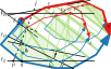
Figure 2: Rotating tangent lines $\ell_{R}$ and $\ell_{B}$ around $P$ while the lines touch points $r$ and $b$ matched by the green matching.

Lemma 2.1.

For any matching $(f,g)$ between $R$ and $B$, there exists a value $t\in[0,1]$ and parallel lines tangent to $R(f(t))$ and $B(g(t))$ with $P$ in the area between them.

Proof 2.2.

Let $\ell_{R}$ and $\ell_{B}$ be two coinciding lines tangent to $P$ at $R(1)=B(1)$. Due to the continuous and monotonic nature of matchings, we can rotate $\ell_{R}$ and $\ell_{B}$ clockwise and counter-clockwise, respectively, around $P$, until they coincide again, such that at every point of the movement, there are points $r\in\ell_{R}$ and $b\in\ell_{B}$ that are matched by $(f,g)$. See Figure˜2 for an illustration. Because the lines start and end as coinciding tangents, there must be a point in time strictly between the start and end of the movement where the lines are parallel. The area between these lines contains $P$, and thus these lines specify a time $t\in[0,1]$ that satisfies the claim.

Lemma 2.3.

There exists a Fréchet matching between $R$ and $B$ that is a maximally-parallel matching with respect to a line perpendicular to an edge of $P$.

Proof 2.4.

Let $(f,g)$ be an arbitrary Fréchet matching. Consider two parallel tangents $\ell_{R}$ and $\ell_{B}$ of $P$ with $P$ between them, such that exists a $t\in[0,1]$ for which $R(f(t))$ lies on $\ell_{R}$ and $B(g(t))$ lies on $\ell_{B}$. Such tangents exist by Lemma˜2.1. Let $r^{*}\in\ell_{R}\cap R$ and $B(y)\in\ell_{B}\cap B$ form a bichromatic closest pair of points and let $\ell^{*}$ be the line through them. We show that the maximally-parallel matching $(f^{*},g^{*})$ with respect to $\ell^{*}$ is a Fréchet matching

Let $R[r,r^{\prime}]$ and $B[b,b^{\prime}]$ be the maximal subcurves for which the lines supporting $\overline{rb}$ and $\overline{r^{\prime}b^{\prime}}$ are parallel to $\ell$, and $R[r,r^{\prime}]$ and $B[b,b^{\prime}]$ are contained in the strip bounded by these lines. The parallel part of $(f^{*},g^{*})$ matches $R[r,r^{\prime}]$ to $B[b,b^{\prime}]$ such that for every pair of points matched, the line through them is parallel to $\ell^{*}$. For every pair of matched points $\hat{r}\in R[r,r^{\prime}]$ and $\hat{b}\in B[b,b^{\prime}]$, we naturally have $d(\hat{r},\hat{b})\leq d(r^{*},b^{*})$. By virtue of $r^{*}$ and $b^{*}$ forming a bichromatic closest pair among all points on $\ell_{R}\cap R$ and $\ell_{B}\cap B$, we additionally have $d(r^{*},b^{*})\leq d(R(f(t)),B(g(t)))\leq d_{\mathrm{F}}(R,B)$. Hence the parallel part has a cost of at most $d_{\mathrm{F}}(R,B)$.

Figure 3: An illustration of the various points and lines used in Lemma˜2.3.

Next we prove that the costs of the first and last fans of $(f^{*},g^{*})$ are at most $d_{\mathrm{F}}(R,B)$. We prove this for the first fan, which matches the prefix of $R$ up to $r$ to the prefix of $B$ up to $b$; the proof for the other fan is symmetric. We assume without loss of generality that $r=R(1)$, so $(f^{*},g^{*})$ matches $r$ to the entire prefix of $B$ up to $b$. Let $r_{t}=R(f(t))$ and $b_{t}=B(g(t))$. See Figure˜3 for an illustration of the various points and lines used.

Let $\hat{\ell}$ (respectively $\bar{\ell}$) be the line through $r$ that is parallel (respectively perpendicular) to the line through $r_{t}$ and $b_{t}$. The lines $\hat{\ell}$ and $\bar{\ell}$ divide the plane into four quadrants. Let $\hat{B}$ be the maximum prefix of $B$ that is interior-disjoint from $\hat{\ell}$. The subcurves $R[1,f(t)]$ and $\hat{B}$ lie in opposite quadrants. Hence for each point on $\hat{B}$, its closest point on $R[1,f(t)]$ is $r$. Since $b_{t}$ does not lie interior to $\hat{B}$, the Fréchet matching $(f,g)$ matches all points on $\hat{B}$ to points on $R[1,f(t)]$. It follows that the cost of matching $r$ to all of $\hat{B}$ is at most $d_{\mathrm{F}}(R,B)$.

To finish our proof we show that the cost of matching $r$ to the subcurve $B^{\prime}$, starting at the last endpoint of $\hat{B}$ and ending at $b$, is at most $d_{\mathrm{F}}(R,B)$. We consider two triangles. The first triangle, $\Delta$, is the triangle with vertices at $r_{t}$, $b_{t}$, and $b^{*}$. For the second triangle, let $p$ be the point on $\ell_{B}$ for which $\overline{rp}$ lies on $\bar{\ell}$, and let $q$ be the point on $\ell_{B}$ for which $b\in\overline{rq}$. We define the triangle $\hat{\Delta}$ to be the triangle with vertices at $r$, $p$, and $q$. The two triangles $\Delta$ and $\hat{\Delta}$ are similar, with $\Delta$ having longer edges. Given that $\overline{r_{t}b_{t}}$ is the longest edge of $\Delta$, it follows that all points in $\Delta$ are within distance $d(R(f(t)),B(g(t)))\leq d_{\mathrm{F}}(R,B)$ of $r_{t}$. By similarity we obtain that all points in $\hat{\Delta}$ are within distance $d_{\mathrm{F}}(R,B)$ of $r$. The subcurve $B^{\prime}$ lies inside $\hat{\Delta}$, so the cost of matching $r$ to all of $B^{\prime}$ is at most $d_{\mathrm{F}}(R,B)$. This proves that the cost of the first fan, matching $r$ to the prefix of $B$ up to $b$, is at most $d_{\mathrm{F}}(R,B)$.

Next we give a linear-time algorithm for constructing a maximally-parallel Fréchet matching. First, note that there are only $\mathcal{O}(n+m)$ maximally-parallel matchings of the form given in Lemma˜2.3 (up to reparameterizations). This is due to the fact that there are only $\mathcal{O}(n+m)$ pairs of parallel tangents of $P$ whose intersection with $P$ is distinct [20]. With the method of [20] (nowadays referred to as “rotating calipers”), we enumerate this set of pairs in $\mathcal{O}(n+m)$ time.

We consider only the pairs of lines $\ell_{R}$ and $\ell_{B}$ where $\ell_{R}$ touches $R$ and $\ell_{B}$ touches $B$. Let $(\ell_{R,1},\ell_{B,1}),\dots,(\ell_{R,k},\ell_{B,k})$ be the considered pairs. For each considered pair of lines $\ell_{R,i}$ and $\ell_{B,i}$, we take a bichromatic closest pair formed by points $r^{*}_{i}\in\ell_{R,i}\cap R$ and $b^{*}_{i}\in\ell_{B,i}$. We assume that the pairs of lines are ordered such that for any $i\leq i^{\prime}$, $r^{*}_{i}$ comes before $r^{*}_{i^{\prime}}$ along $R$ and $b^{*}_{i}$ comes after $b^{*}_{i^{\prime}}$ along $B$. We let $(f_{i},g_{i})$ be the maximally-parallel matching with respect to the line through $r^{*}_{i}$ and $b^{*}_{i}$. By Lemma˜2.3, one of these matchings is a Fréchet matching. To determine which matching is a Fréchet matching, we compute the costs of the three parts (the first fan, the parallel part, and the last fan) of each matching $(f_{i},g_{i})$.

The cost of the parallel part of $(f_{i},g_{i})$ is equal to $d(r^{*}_{i},b^{*}_{i})$. We compute these costs in $\mathcal{O}(n+m)$ time altogether. For the costs of the first fans, suppose without loss of generality that there exists an integer $j$ for which the first fan of $(f_{i},g_{i})$ matches $R(1)$ to a prefix of $B$ for all $i\leq j$, and matches $B(1)$ to a prefix of $R$ for all $i>j$. As $i$ increases from $1$ to $j$, the prefix of $B$ matched to $R(1)$ shrinks. Through a single scan over $B$, we compute the cost function $y\mapsto\max_{\hat{y}\in[1,y]}d(R(1),B(\hat{y}))$, which measures the cost of matching $R(1)$ to any given prefix of $B$. This function is piecewise hyperbolic with a piece for every edge of $B$. Constructing the function takes $\mathcal{O}(m)$ time, and allows for computing the cost of matching any given prefix to $R(1)$ in constant time. We compute the first fan of $(f_{i},g_{i})$ for all $i\leq j$ in $\mathcal{O}(m)$ time by scanning backwards over $B$. Extracting the costs of these fans then takes $\mathcal{O}(j)$ additional time in total.

Through a procedure symmetric to the above, we compute the cost of the first fan of $(f_{i},g_{i})$ for all $i>j$ in $\mathcal{O}(n)$ time altogether, through two scans of $R$. Thus, the cost of all first fans, and by symmetry the costs of the last fans, can be computed in $\mathcal{O}(n+m)$ time. Taking the maximum between the costs of the first fan, the parallel part, and the last fan, for each matching $(f_{i},g_{i})$, we obtain the cost of the entire matching. Picking the cheapest matching yields a Fréchet matching between $R$ and $B$.

Theorem 2.5.

Let $R\colon[1,n]\to\mathbb{R}^{2}$ and $B\colon[1,m]\to\mathbb{R}^{2}$ be two simple curves bounding a convex polygon, with $R(1)=B(1)$ and $R(n)=B(m)$. We can construct a Fréchet matching between $R$ and $B$ in $\mathcal{O}(n+m)$ time.

3 Approximate geodesic Fréchet distance

In this section we describe our approximation algorithm. Let $\varepsilon>0$ be a parameter. Our algorithm computes a $(1+\varepsilon)$-approximation to the geodesic Fréchet distance $d_{\mathrm{F}}(R,B)$. It makes use of a $(1+\varepsilon)$-approximate decision algorithm. Here we are given an additional parameter $\delta\geq 0$, and report either that $d_{\mathrm{F}}(R,B)\leq(1+\varepsilon)\delta$ or that $d_{\mathrm{F}}(R,B)>\delta$. If $\delta<d_{\mathrm{F}}(R,B)\leq(1+\varepsilon)\delta$, we may report either answer. In our setting of the problem, we show that the geodesic Fréchet distance is approximately the geodesic Hausdorff distance between $R$ and $B$, that is, at most three times as large. The geodesic Hausdorff distance can be computed in $\mathcal{O}((n+m)\log nm)$ time [10, Theorem 7.1] and gives an accurate guess $\overline{\delta}$ of the Fréchet distance. We then perform binary search over the values $\overline{\delta},(1+\varepsilon)\overline{\delta},\dots,3\overline{\delta}$ and apply our approximate decision algorithm at each step (see Section 3.4). This proves the following theorem:

Theorem 3.1.

Let $R\colon[1,n]\to\mathbb{R}^{2}$ and $B\colon[1,m]\to\mathbb{R}^{2}$ be two simple curves bounding a simple polygon, with $R(1)=B(1)$ and $R(n)=B(m)$. Let $\varepsilon>0$ be a parameter. We can compute a $(1+\varepsilon)$-approximation to $d_{\mathrm{F}}(R,B)$ in $\mathcal{O}(\frac{1}{\varepsilon}(n+m\log n)\log nm\log\frac{1}{\varepsilon})$ time.

In the remainder of this section we focus on our approximate decision algorithm. At its heart lies a useful connection between matchings and nearest neighbors: for a point $r$ on $R$ its nearest neighbors are the points $b$ on $B$ closest to it. Any $\delta$-matching must match a nearest neighbor $b$ relatively close to $r$. Specifically, we prove in Section˜3.1 that $b$ must be matched to a point $r^{\prime}$ for which all points between $r$ and $r^{\prime}$ are within distance $\delta$ of $b$. We capture this relation using $(r,b,\delta)$-nearest neighbor fans. A nearest neighbor fan $F_{r,b}(\delta)$ corresponds to the point $b$ and the maximal subcurve $R[x,x^{\prime}]$ that contains $r$ and is within geodesic distance $\delta$ of $b$; it is the union of geodesics between $b$ and points on $R[x,x^{\prime}]$

As $r$ moves monotonically along $R$, so do its nearest neighbors $b$ along $B$, together with their nearest neighbor fan $F_{r,b}(\delta)$. While $r$ moves continuously along $R$, the points $b$ and their fans might jump discontinuously. We show in Section 3.2 how to use the matchings from the fans to efficiently answer the decision question for those points that are part of the fans. For sufficiently large values of $\delta$, which includes $\delta=\overline{\delta}$, every point on $R$ is part of a nearest neighbor fan. We distinguish the points on $B$ based on whether they are a nearest neighbor of a point on $R$. The points that are a nearest neighbor are called near points, and others are called far points. On $B$, the near points are part of a nearest neighbor fan, but the far points are not. Far points pose the greatest technical challenge for our algorithm; in Section 3.3 we show how to construct a $\delta$-matching for far points in an approximate manner.

Specifically, let $b,b^{\prime}\in B$ be two points that are involved in nearest neighbor fans, but all points strictly between $b$ and $b^{\prime}$ are not, that is, they are far points. There must be a point $r\in R$ for which both $b$ and $b^{\prime}$ are nearest neighbors and hence $d(b,b^{\prime})\leq 2d_{\mathrm{F}}(R,B)$. In other words, the geodesic from $b$ to $b^{\prime}$ is short and separates $R$ from the subcurve $B[b,b^{\prime}]$. We are going to use this separating geodesic to transform the decision problem for far points into $K=\mathcal{O}(1/\varepsilon)$ one-dimensional problems.

Specifically, we discretize the separator with $K$ points, which we call anchors, and ensure that consecutive ones have distance at most $\varepsilon\delta$ between them. We snap our geodesics to these anchors, which incurs a small approximation error. Based on which anchor point a geodesic snaps to, we partition the product parameter space of $R$ and $B^{\prime}$ into regions, one for each anchor point. For each anchor point, the lengths of these geodesics snapped to it can be described as the distances between points on two separated one-dimensional curves; this is exactly the one-dimensional problem we now need to solve exactly. Section 3.3 explains the transformation in detail and in Section 4 we show how to solve the exact one-dimensional problem efficiently.

3.1 Nearest neighbor fans

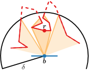
Figure 4: (left) Points $r$ and $b$ with $b\in\mathit{NN}(r)$. The non-dashed red subcurves of $R$ are within geodesic distance $\delta$ of $b$. (right) The $(r,b,\delta)$-nearest neighbor fan.

Let $\mathit{NN}(r)$ denote the set of nearest neighbors of a point $r\in R$ with respect to $B$. That is, $\mathit{NN}(r)$ is the set of points $b\in B$ with $d(r,b)\leq d(r,b^{\prime})$ for any $b^{\prime}\in B$. For $b\in\mathit{NN}(r)$, let $R[x,x^{\prime}]$ be the maximal subcurve containing $r$ that is within geodesic distance $\delta$ of $b$. The $(r,b,\delta)$-nearest neighbor fan $F_{r,b}(\delta)$ is the union of geodesics between points on $R[x,x^{\prime}]$ and $b$ (see Figure˜4). We call $b$ the apex of $F_{r,b}(\delta)$ and $R[x,x^{\prime}]$ the leaf of $F_{r,b}(\delta)$.

In Lemma 3.4 we prove a crucial property of nearest neighbor fans, namely that any $\delta$-matching between $R$ and $B$ matches $b$ to a point on the leaf of the fan. For the proof, we make use of the following auxiliary lemma:

Lemma 3.2.

Let $r\in R$ and $b\in\mathit{NN}(r)$. For any points $r^{\prime}\in R$ and $b^{\prime}\in B$ on opposite sides of $\pi(r,b)$, we have $d(r^{\prime},b)\leq d(r^{\prime},b^{\prime})$.

Proof 3.3.

All points $p$ on $\pi(r,b)$ naturally have the property that $d(p,b)\leq d(p,b^{\prime})$ for all $b^{\prime}\in B$. For any $r^{\prime}\in R$ and $b^{\prime}\in B$ on opposite sides of $\pi(r,b)$, the geodesic $\pi(r^{\prime},b^{\prime})$ intersects $\pi(r,b)$ in a point $p$. It follows from the triangle inequality that

$$d(r^{\prime},b) \leq d(r^{\prime},p)+d(p,b)$$

$$\leq d(r^{\prime},p)+d(p,b^{\prime})=d(r^{\prime},b^{\prime}).$$

Lemma 3.4.

Let $r\in R$ and $b\in\mathit{NN}(r)$. For any $\delta\geq 0$, every $\delta$-matching between $R$ and $B$ matches $b$ to a point in the leaf of $F_{r,b}(\delta)$.

Proof 3.5.

Suppose $b$ is matched to a point $r^{\prime}$ by some $\delta$-matching $(f,g)$. Assume without loss of generality that $r^{\prime}$ comes before $r$ along $R$. Let $\hat{r}$ be a point between $r^{\prime}$ and $r$. The $\delta$-matching $(f,g)$ matches $\hat{r}$ to a point $\hat{b}$ after $b$. Thus we obtain from Lemma˜3.2 that $d(\hat{r},b)\leq d(\hat{r},\hat{b})\leq\delta$. This proves that all points between $r^{\prime}$ and $r$ are included in the leaf of $F_{r,b}(\delta)$.

An important consequence of Lemma˜3.4 is that if $b=B(y)\in\mathit{NN}(r)$ and $R(x)$ is the first point in the leaf of $F_{r,b}(\delta)$ for which $d_{\mathrm{F}}(R[1,x],B[1,y])\leq\delta$, then there exists a $\delta$-matching (if any exist at all) that matches $R(x)$ to $B(y)$.

We further investigate the structure of $F_{r,b}(\delta)$ and its connection to $\delta$-matchings. Namely, we show that the $(r,b,\delta)$-nearest neighbor fans are monotonic with respect to their apexes, in a sense that suits matchings well. We make the assumption that there is no nearest neighbor fan $F_{r,b}(\delta)$ with an empty leaf, which in particular means that $d(r,b)\leq\delta$. If $F_{r,b}(\delta)$ does have an empty leaf, we say that the nearest neighbor fan is empty (which is also reflected in the fact that it is the union of $0$ geodesics).

Lemma 3.6.

Suppose there are no empty nearest neighbor fans. Let $r$ and $r^{\prime}$ be points on $R$ and let $b\in\mathit{NN}(r)$ and $b^{\prime}\in\mathit{NN}(r^{\prime})$. Let $R[x_{1},x_{2}]$ and $R[x^{\prime}_{1},x^{\prime}_{2}]$ be the leaves of $F_{r,b}(\delta)$ and $F_{r^{\prime},b^{\prime}}(\delta)$. If $b$ comes before $b^{\prime}$, then $x_{1}\leq x^{\prime}_{1}$ and $x_{2}\leq x^{\prime}_{2}$.

Proof 3.7.

Suppose by way of contradiction that $x_{1}>x^{\prime}_{1}$. We naturally have that $R(x_{1})$ comes before $r$, and thus $R(x^{\prime}_{1})$ comes before $r$. The subcurve $R[x^{\prime}_{1},x_{1}]$ and the point $b^{\prime}$ therefore lie on opposite sides of $\pi(r,b)$. It therefore follows from Lemma˜3.2 that $d(\hat{r},b)\leq d(\hat{r},b^{\prime})\leq\delta$ for all $\hat{r}\in R[x^{\prime}_{1},x_{1}]$. By maximality of the leaf of $F_{r,b}$, we thus must have that $R[x^{\prime}_{1},x_{1}]$ is part of the leaf, contradicting the fact that $R[x_{1},x_{2}]$ is the leaf.

Denote by $\mathcal{B}=\bigcup_{r\in R}\mathit{NN}(r)\subseteq B$ the set of all near points, and recall that each near point is the apex of a nearest neighbor fan. We give a strong property regarding matchings and points interior to the connected components of $\mathcal{B}$:

Lemma 3.8.

Suppose there are no empty nearest neighbor fans. Let $b=B(y)$ and $b^{\prime}=B(y^{\prime})$ be in the same connected component of $\mathcal{B}$, with $y\leq y^{\prime}$. Let $R[x_{1},x_{2}]$ and $R[x^{\prime}_{1},x^{\prime}_{2}]$ be the leaves of $F_{r,B(y)}(\delta)$ and $F_{r^{\prime},B(y^{\prime})}(\delta)$, respectively. If $d_{\mathrm{F}}(R[1,x],B[1,y])\leq\delta$ for some $x\in[x_{1},x_{2}]$, then $d_{\mathrm{F}}(R[1,\max\{x,x^{\prime}_{1}\}],B[1,y^{\prime}])\leq\delta$.

Proof 3.9.

Let $b\in\mathit{NN}(r)$ and $b^{\prime}\in\mathit{NN}(r^{\prime})$ for some $r,r^{\prime}\in R$. Because $b$ and $b^{\prime}$ are in the same connected component of $\mathcal{B}$, every $\hat{b}\in B$ between $b$ and $b^{\prime}$ is the apex of a nearest neighbor fan $F_{\hat{r},\hat{b}}(\delta)$. Lemma˜3.2 implies that as $\hat{b}$ moves along $B$ from $b$ to $b^{\prime}$, $\hat{r}$ moves along $R$ from $r$ to $r^{\prime}$.

Since there are no empty nearest neighbor fans, each $\hat{r}$ is contained in the leaf of $F_{\hat{r},\hat{b}}(\delta)$. Thus every point on $R[x,\max\{x,x^{\prime}_{1}\}]$ is contained in some leaf. By Lemma˜3.6 we can move along $R[x,\max\{x,x^{\prime}_{1}\}]$ while staying inside the leaf of $F_{\hat{r},\hat{b}}(\delta)$ by moving $\hat{b}$ along $B$.

3.2 Approximate decision algorithm

In this section we give a $(1+\varepsilon)$-approximate decision algorithm. Given $\delta\geq 0$ and $\varepsilon>0$, our algorithm reports that $d_{\mathrm{F}}(R,B)\leq(1+\varepsilon)\delta$ or $d_{\mathrm{F}}(R,B)>\delta$. Throughout this section, we assume that $\delta\geq\max_{r\in R}\min_{b\in B}d(r,b)$, that is, there are no empty nearest neighbor fans. This is a natural assumption, as the geodesic Fréchet distance is bounded below by the maximum nearest neighbor distance. We compute this lower bound, which is the directed Hausdorff distance, in $\mathcal{O}((n+m)\log nm)$ time with the algorithm of Cook and Wenk [10].

Our algorithm considers a point $r$ that monotonically traverses the entirety of $R$. As it does so, its nearest neighbors $b\in\mathit{NN}(r)\subseteq\mathcal{B}$ monotonically traverse all the near points $\mathcal{B}\subseteq B$. For each near point $b\in\mathit{NN}(r)$, we either decide that there is a point $\hat{r}$ on $R$ for which there exists a $(1+\varepsilon)\delta$-matching from $(1,1)$ to $(\hat{r},b)$, or discover that a $\delta$-matching between $R$ and $B$ does not exist. Specifically, consider a connected component $B[y,y^{\prime}]$ of $\mathcal{B}$ and let $B(y)\in\mathit{NN}(r)$ and $B(y^{\prime})\in\mathit{NN}(r^{\prime})$ for some $r,r^{\prime}\in R$. Let $R[x_{1},x_{2}]$ and $R[x^{\prime}_{1},x^{\prime}_{2}]$ be the leaves of $F_{r,B(y)}(\delta)$ and $F_{r^{\prime},B(y^{\prime})}(\delta)$, respectively. Suppose that $d_{\mathrm{F}}(R[1,x],B[1,y])\leq\delta$ for some $x\in[x_{1},x_{2}]$. Then Lemma˜3.8 implies that $d_{\mathrm{F}}(R[1,x^{*}],B[1,y^{\prime}])\leq\delta$ for $x^{*}=\max\{x,x^{\prime}_{1}\}$. See Figure˜5. Hence, it is sufficient to construct the fans only for the endpoints $B(y)$ and $B(y^{\prime})$ of each connected component of $\mathcal{B}$ together with the first points on $R$ that they can be matched to by a $\delta$-matching.

Figure 5: (left) The $(r,b,\delta)$-nearest neighbor fans correspond to a bimonotone region in the $\delta$-free space. The middle partly-dashed curve indicates the nearest neighbor(s) on $B$ of points on $R$. (right) There is a matching that moves vertically upwards whenever possible. In the dashed rectangles, $B$ has only far points, and the matching becomes more complex.

Lemma 3.10.

We can construct the fans $F_{r,b}(\delta)$ for all endpoints $b$ of connected components of $\mathcal{B}$ in $\mathcal{O}((n+m)\log nm)$ time in total.

Proof 3.11.

We first construct the geodesic Voronoi diagram $\mathcal{V}_{P}(B)$ of $B$ inside $P$. This diagram is a partition of $P$ into regions containing those points for which the closest edge(s) of $B$ (under the geodesic distance) are the same. Points inside a cell have only one edge of $B$ closest to them, whereas points on the segments and arcs bounding the cells have multiple. The geodesic Voronoi diagram can be constructed in $\mathcal{O}((n+m)\log nm)$ time with the algorithm of Hershberger and Suri [19].

The points on $R$ that lie on the boundary of a cell of $\mathcal{V}_{P}(B)$ are precisely those that have multiple (two) points on $B$ closest to them. By general position assumptions, these points form a discrete subset of $R$. Furthermore, there are only $\mathcal{O}(m)$ such points. We identify these points $r$ by scanning over $\mathcal{V}_{P}(B)$. From this, we also get the two edges of $B$ containing $\mathit{NN}(r)$, and we compute the set $\mathit{NN}(r)$ in $\mathcal{O}(\log nm)$ time with the data structure of [10, Lemma 3.2] (after $\mathcal{O}(n+m)$-time preprocessing). The sets $\mathit{NN}(r)$ with cardinality two are precisely the ones containing the endpoints of connected components of $\mathcal{B}$.

We consider the endpoints of connected components of $\mathcal{B}$ in their order along $B$. For each endpoint $b$ with $b\in\mathit{NN}(r)$, we construct the last point in the leaf of $F_{r,b}(\delta)$. By a symmetric procedure, where we consider the endpoints of $\mathcal{B}$ in the reverse order along $B$, the first points of the leaves can be computed.

We first compute the last point in the leaf of $F_{R(1),B(1)}$. For this, we compute the first vertex $r_{i}$ of $R$ with $d(r_{i},B(1))>\delta$. We do so in $\mathcal{O}(i\log nm)$ time by scanning over the vertices of $R$. For any edge $\overline{r_{i^{\prime}}r_{i^{\prime}+1}}$ of $R$, the distance $d(r,B(1))$ as $r$ varies from $r_{i^{\prime}}$ to $r_{i^{\prime}+1}$ first decreases monotonically to a global minimum and then increases monotonically [10, Lemma 2.1]. Thus $d(r,B(1))\leq\delta$ for all $r\in R[1,i-1]$. Moreover, the last point in the leaf of $F_{R(1),B(1)}(\delta)$ is the last point on $\overline{r_{i-1}r_{i}}$ with geodesic distance $\delta$ to $B(1)$. We compute this point in $\mathcal{O}(\log nm)$ time with the data structure of [10, Lemma 3.2].

Next we compute the last point in the leaf of $F_{r,b}(\delta)$, where $b$ is the next endpoint of a connected component of $\mathcal{B}$ and $b\in\mathit{NN}(r)$. Let $r^{*}=R(x^{*})$ be the last point in the leaf of $F_{R(1),B(1)}(\delta)$. From the monotonicity of the fan leaves (Lemma˜3.6), the last point in the leaf of $F_{r,b}(\delta)$ comes after $r^{*}$ along $R$. Let $r=R(x)$ and $b=B(y)$. Given that $r$ is contained in the leaf of $F_{r,b}(\delta)$ (by our assumption that there are no empty nearest neighbor fans), the point we are looking for lies on $R[\max\{x^{*},x\},n]$. We proceed as before, setting $R$ to be its subcurve $R[\max\{x^{*},x\},n]$ and $B$ to be its subcurve $B[y,m]$.

The above iterative procedure takes $\mathcal{O}((n+|\mathcal{B}|)\log nm)$ time, where $|\mathcal{B}|=\mathcal{O}(m)$ is the number of connected components of $\mathcal{B}$. This running time is subsumed by the $\mathcal{O}((n+m)\log n\log nm)$ time taken to construct $\mathcal{B}$.

It remains to handle the far points, that is, $B\setminus\mathcal{B}$. Consider a maximal subcurve $B^{\prime}=B[y,y^{\prime}]$ with only far points on its interior. Let $R[x_{1},x_{2}]$ and $R[x^{\prime}_{1},x^{\prime}_{2}]$ be the leaves of $F_{r,B(y)}(\delta)$ and $F_{r^{\prime},B(y^{\prime})}(\delta)$, respectively. Let $R(x^{*})\in R[x^{\prime}_{1},x^{\prime}_{2}]$ be the first point for which $d_{\mathrm{F}}(R[1,x^{*}],B[1,y^{\prime}])\leq\delta$. We seek to compute some $\hat{x}\in[x^{\prime}_{1},x^{*}]$ such that $d_{\mathrm{F}}(R[1,\hat{x}],B[1,y^{\prime}])\leq(1+\varepsilon)\delta$, so that we can continue the matching from $(\hat{x},y^{\prime})$. We do so using an approximate algorithm that we develop in Section˜3.3.

The time spent computing $\hat{x}$ is $\mathcal{O}(\frac{1}{\varepsilon}(|R[x_{1},\hat{x}]|+|B^{\prime}|\log n)\log nm)$, after $\mathcal{O}(n+m)$-time preprocessing. There are only $\mathcal{O}(m)$ maximal subcurves $B^{\prime}$ of $B$ with only far points on their interior. Hence taken over all such subcurves, the time spent on our algorithm of Section˜3.3 is $\mathcal{O}(\frac{1}{\varepsilon}(n+m\log n)\log nm)$.

Theorem 3.12.

Let $R\colon[1,n]\to\mathbb{R}^{2}$ and $B\colon[1,m]\to\mathbb{R}^{2}$ be two simple curves bounding a simple polygon, with $R(1)=B(1)$ and $R(n)=B(m)$. Let $\delta\geq 0$ and $\varepsilon>0$ be parameters. If $\delta\geq\min_{r\in R}\max_{b\in B}d(r,b)$, then we can decide whether $d_{\mathrm{F}}(R,B)\leq(1+\varepsilon)\delta$ or $d_{\mathrm{F}}(R,B)>\delta$ in $\mathcal{O}(\frac{1}{\varepsilon}(n+m\log n)\log nm)$ time.

3.3 Matching far points

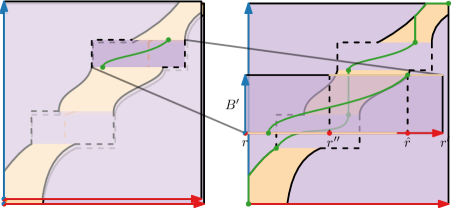
Figure 6: The subproblem of matching far points.

The input for our algorithm that we describe in this section is a subcurve $B^{\prime}$ of $B$ that contains only far points in its interior, and three points $r,r^{\prime\prime},r^{\prime}$ that occur in this order on $R$. The algorithm computes a point $\hat{r}$ on $R[r^{\prime\prime},r^{\prime}]$ such that $R[r,\hat{r}]$ can be $(1+\varepsilon)\delta$-matched to $B^{\prime}$ (if such a point exists). Furthermore, if there exists a last point $r^{*}$ on $R[r^{\prime\prime},r^{\prime}]$ for which $R[r,r^{*}]$ can be $\delta$-matched to $B^{\prime}$, then $\hat{r}$ comes before $r^{*}$ on $R$. This point $\hat{r}$ is the one we use in Section˜3.2 to continue the matching after $B^{\prime}$. See Figure˜6 for an illustration.

We first describe an approximate decision algorithm that, given $\hat{r}$, reports whether $d_{\mathrm{F}}(R[r,\hat{r}],B^{\prime})\leq(1+\varepsilon)\delta$ or $d_{\mathrm{F}}(R[r,\hat{r}],B^{\prime})>\delta$. Let $R^{\prime}=R[r,\hat{r}]$ and $B^{\prime}=B[b,b^{\prime}]$. There is a point $\overline{r}$ on $R$ with $\mathit{NN}(\overline{r})=\{b,b^{\prime}\}$, which implies that $d(b,b^{\prime})\leq d(b,\overline{r})+d(\overline{r},b^{\prime})\leq 2\delta$. Thus the geodesic $\pi(B^{\prime})$ that connects $b$ to $b^{\prime}$ has length at most $2\delta$ and is hence a short separator between $R^{\prime}$ and $B^{\prime}$.

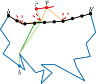
Figure 7: (left) The points $b$ and $b^{\prime}$ are closest to $\overline{r}$. The geodesic $\pi(B^{\prime})=\pi(b,b^{\prime})$ has length at most $2\delta$. (right) Rerouting $\pi(\tilde{r},\tilde{b})$ through an anchor, increasing its length by at most $\varepsilon\delta$.

We discretize $\pi(B^{\prime})$ with $K=\mathcal{O}(1/\varepsilon)$ points $p_{1},\dots,p_{K}$, which we call anchors, and ensure that consecutive anchors have distance at most $\varepsilon\delta$ between them (see Figure˜7 (right)). We assume that no anchor coincides with a vertex of $R^{\prime}$ and $B^{\prime}$. Furthermore, we assume that for every edge $e$ of $R^{\prime}$, with $\tilde{r}\in e$ closest to an anchor $p_{k}$, there is a unique point $\tilde{b}\in B^{\prime}$ for which $\pi(\tilde{r},\tilde{b})$ goes through $p_{k}$. We assume a symmetric statement with respect to edges of $B$. These assumptions are easily satisfied by perturbing the anchors along $\pi(B^{\prime})$, possibly adding an extra anchor.

If a geodesic $\pi(\tilde{r},\tilde{b})$ intersects $\pi(B^{\prime})$ between consecutive anchors $p_{k}$ and $p_{k+1}$, then $d(\tilde{r},\tilde{b})\leq d(\tilde{r},p_{k})+d(p_{k},\tilde{b})\leq d(\tilde{r},\tilde{b})+\varepsilon\delta$. We can hence approximate the geodesic between $\tilde{r}$ and $\tilde{b}$ by “snapping” it to $p_{k}$; that is, replacing it by the geodesics $\pi(\tilde{r},p_{k})$ and $\pi(\tilde{b},p_{k})$ (see Figure˜7 (right)).

We now turn to the parameter space of $R^{\prime}$ and $B^{\prime}$. Here, the set of geodesics $\pi(R^{\prime}(x),B^{\prime}(y))$ that go through an anchor $p_{k}$ corresponds to a bimonotone path. We identify a set $S_{k}$ of $\mathcal{O}(n+m)$ points on this bimonotone path, such that there exists a $\delta$-matching that goes through a point of $S_{k}$ for all $k$.

To define the sets $S_{k}$, we make use of a particular (unknown) Fréchet matching between the (original) curves $R$ and $B$. Namely, a Fréchet matching that matches points either to vertices of the other curve, or to locally closest points. We say that a point $\tilde{r}$ on $R$ is locally closest to a point $\tilde{b}$ on $B$ if perturbing $\tilde{r}$ infinitesimally while staying on $R$ increases its distance to $\tilde{b}$. We analogously say that $\tilde{b}$ is locally closest to $\tilde{r}$ if perturbing $\tilde{b}$ infinitesimally while staying on $B$ increases its distance to $\tilde{r}$.

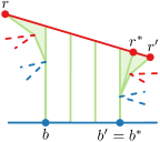
Figure 8: The construction in Lemma˜3.13. Non-dashed segments are $\overline{r_{i}r_{i+1}}$ and $\overline{b_{j}b_{j+1}}$.

Lemma 3.13.

There exists a Fréchet matching between $R$ and $B$ where for every matched pair $(\tilde{r},\tilde{b})$, at least one of $\tilde{r}$ and $\tilde{b}$ is a vertex, or locally closest to the other point.

Proof 3.14.

Let $(f,g)$ be a Fréchet matching between $R$ and $B$. Based on $(f,g)$, we construct a new Fréchet matching $(f^{\prime},g^{\prime})$ that satisfies the claim.

For each vertex $r_{i}$ of $R$, if $(f,g)$ matches it to a point interior to an edge $\overline{b_{j}b_{j+1}}$ of $B$, or to the vertex $b_{j}$, then we let $(f^{\prime},g^{\prime})$ match $r_{i}$ to the point on $\overline{b_{j}b_{j+1}}$ closest to it. This point is either $b_{j}$, $b_{j+1}$, or it is locally closest to $r_{i}$. Symmetrically, for each vertex $b_{j}$ of $B$, if $(f,g)$ matches it to a point interior to an edge $\overline{r_{i}r_{i+1}}$ of $R$, or to the vertex $r_{i+1}$, then we let $(f^{\prime},g^{\prime})$ match $b_{j}$ to the point on $\overline{r_{i}r_{i+1}}$ closest to it. This point is either a vertex or locally closest to $b_{j}$.

Consider two maximal subsegments $\overline{rr^{\prime}}$ and $\overline{bb^{\prime}}$ of $R$ and $B$ where currently, $r$ is matched to $b$ and $r^{\prime}$ is matched to $b^{\prime}$. See Figure˜8 for an illustration of the following construction. Let $\overline{rr^{\prime}}\subseteq\overline{r_{i}r_{i+1}}$ and $\overline{bb^{\prime}}\subseteq\overline{b_{j}b_{j+1}}$. We have $r=r_{i}$ or $b=b_{j}$, as well as $r^{\prime}=r_{i+1}$ or $b^{\prime}=b_{j+1}$.

Let $r^{*}\in\overline{rr^{\prime}}$ and $b^{*}\in\overline{bb^{\prime}}$ minimize the geodesic distance $d(r^{*},b^{*})$ between them. It is clear that $r^{*}$ and $b^{*}$ are both either vertices or locally closest to the other point. We let $(f^{\prime},g^{\prime})$ match $r^{*}$ to $b^{*}$. Since $(f,g)$ originally matched $r^{*}$ and $b^{*}$ to points on $\overline{r_{i}r_{i+1}}$ and $\overline{b_{j}b_{j+1}}$, respectively, we have $d(r^{*},b^{*})\leq d_{\mathrm{F}}(R,B)$. Next we define the part of $(f^{\prime},g^{\prime})$ that matches $\overline{rr^{*}}$ to $\overline{bb^{*}}$.

Suppose $r=r_{i}$ and let $\tilde{b}\in\overline{bb^{*}}$ be the point closest to $r$. We let $(f^{\prime},g^{\prime})$ match $r$ to $\overline{b\tilde{b}}$, and match each point on $\overline{rr^{*}}$ to its closest point on $\overline{\tilde{b}b^{*}}$. This is a proper matching, as the closest point on a segment moves continuously along the segment as we move continuously along $R$.

The cost of matching $r$ to $\overline{b\tilde{b}}$ is at most $d(r,b)\leq d_{\mathrm{F}}(R,B)$, since the maximum distance from $r$ to $\overline{b\tilde{b}}$ is attained by $b$ or $\tilde{b}$ [10]. For the cost of matching $\overline{rr^{*}}$ to $\overline{\tilde{b}b^{*}}$, observe that the point on $\overline{\tilde{b}b^{*}}$ closest to a point $\tilde{r}\in\overline{rr^{*}}$ is also the point on $\overline{b_{j}b_{j+1}}$ closest to it. This is due to $\tilde{b}$ being closest to $r$ among the points on $\overline{b_{j}b_{j+1}}$ and $b^{*}$ being locally closest to $r^{*}$, which means it is closest to $r^{*}$ among the points on $\overline{b_{j}b_{j+1}}$. It follows that the cost of matching $\overline{rr^{*}}$ to $\overline{\tilde{b}b^{*}}$ is at most $d_{\mathrm{F}}(R,B)$, since $(f,g)$ matches $\overline{rr^{*}}$ to a subset of $\overline{b_{j}b_{j+1}}$ and $(f^{\prime},g^{\prime})$ matches each point on $\overline{rr^{*}}$ to its closest point on $\overline{b_{j}b_{j+1}}$.

We define a symmetric matching of cost at most $d_{\mathrm{F}}(R,B)$ between $\overline{rr^{*}}$ and $\overline{bb^{*}}$ when $b=b_{j}$. Also, we symmetrically define a matching of cost at most $d_{\mathrm{F}}(R,B)$ between $\overline{r^{*}r^{\prime}}$ and $\overline{b^{*}b^{\prime}}$. The resulting matching $(f^{\prime},g^{\prime})$ satisfies the claim.

Next we define the set $S_{k}$ for an anchor $p_{k}$. By our general position assumption on the anchors, there are only $|R^{\prime}|+|B^{\prime}|$ geodesics $\pi(\tilde{r},\tilde{b})$ through $p_{k}$ that have a vertex of $R^{\prime}$ or $B^{\prime}$ as an endpoint. Additionally, observe that for any geodesic $\pi(\tilde{r},\tilde{b})$ through $p_{k}$, where $\tilde{r}\in\overline{r_{i}r_{i+1}}$ is locally closest to $\tilde{b}$, the point $\tilde{r}$ is also closest to $p_{k}$ among the points on $\overline{r_{i}r_{i+1}}$. Symmetrically, if $\tilde{b}\in\overline{b_{j}b_{j+1}}$ is locally closest to $\tilde{r}$, the point $\tilde{b}$ is also closest to $p_{k}$ among the points on $\overline{b_{j}b_{j+1}}$. This gives $|R^{\prime}|+|B^{\prime}|-2$ geodesics through $p_{k}$ of this form. By Lemma˜3.13 there is a Fréchet matching between $R^{\prime}$ and $B^{\prime}$ that matches a pair of points $\tilde{r}\in R^{\prime}$ and $\tilde{b}\in B^{\prime}$ such that $\pi(\tilde{r},\tilde{b})$ is one of these $2(|R^{\prime}|+|B^{\prime}|)-2$ geodesics. We therefore set $S_{k}$ to be the set of points $(x,y)$ for which $\pi(R^{\prime}(x),B^{\prime}(y))$ is such a geodesic.

Lemma 3.15.

We can construct $S_{k}$ in $\mathcal{O}((|R^{\prime}|+|B^{\prime}|)\log nm)$ time after $\mathcal{O}(n+m)$-time preprocessing.

Proof 3.16.

We make use of three data structures. We preprocess $P$ into the data structure of [16] for shortest path queries, which allows for computing the first edge of $\pi(p,q)$ given points $p,q\in P$ in $\mathcal{O}(\log nm)$ time. We also preprocess $P$ into the data structure of [9] for ray shooting queries, which allows for computing the first point on the boundary of $P$ hit by a query ray in $\mathcal{O}(\log nm)$ time. Lastly, we preprocess $P$ into the data structure of [10, Lemma 3.2], which in particular allows for computing the point on a segment $e$ that is closest to a point $p$ in $\mathcal{O}(\log nm)$ time. The preprocessing time for each data structure is $\mathcal{O}(n+m)$.

Given an edge $\overline{r_{i}r_{i+1}}$ of $R^{\prime}$, we compute the point $\tilde{r}\in\overline{r_{i},r_{i+1}}$ closest to $p_{k}$, as well as the geodesic $\pi(\tilde{r},\tilde{b})$ that goes through $p_{k}$. For this, we first compute the point $\tilde{r}$ in $\mathcal{O}(\log nm)$ time. Then we compute the first edge of $\pi(p_{k},\tilde{r})$ and extend it towards $B^{\prime}$ by shooting a ray from $p_{k}$. This takes $\mathcal{O}(\log nm)$ time. By our general position assumption on the anchors, the ray hits only one point before leaving $P$. This is the point $\tilde{b}$. Through the same procedure, we compute the two geodesics through $p$ that start at $r_{i}$ and $r_{i+1}$, respectively.

Applying the above procedure to all vertices and edges of $R^{\prime}$, and a symmetric procedure to the vertices and edges of $B^{\prime}$, we obtain the set of geodesics corresponding to the points in $S_{k}$. The total time spent is $\mathcal{O}(\log nm)$ per vertex or edge, with $\mathcal{O}(n+m)$ preprocessing time. This sums up to $\mathcal{O}((|R^{\prime}|+|B^{\prime}|)\log nm)$ after preprocessing.

Having constructed the sets $S_{k}$ for all anchors in $\mathcal{O}(\frac{1}{\varepsilon}((|R^{\prime}|+|B^{\prime}|)\log nm)$ time altogether, we move to computing subsets $S^{*}_{k}\subseteq S_{k}$ containing those points that are $\delta$-reachable from $(1,1)$, and only points that are $(1+\varepsilon)\delta$-reachable from $(1,1)$. We proceed iteratively, constructing $S^{*}_{k+1}$ from $S^{*}_{k}$. For this, observe the following. Let $(x,y)\in S^{*}_{k}$ and $(x^{\prime},y^{\prime})\in S_{k+1}$. By definition of the sets $S_{k}$ and $S_{k+1}$, $\pi(R^{\prime}(x),B^{\prime}(y))$ intersects $p_{k}$ and $\pi(R^{\prime}(x^{\prime}),B^{\prime}(y^{\prime}))$ intersects $p_{k+1}$. Hence any geodesic $\pi(\tilde{r},\tilde{b})$ with $\tilde{r}\in R^{\prime}[x,x^{\prime}]$ and $\tilde{b}\in B^{\prime}[y,y^{\prime}]$ intersects the segment $\overline{p_{k}p_{k+1}}$. We may therefore “reroute” all these geodesics to go through $p_{k}$, increasing their length by at most $\varepsilon\delta$.

Let $R_{k}\colon[1,|R^{\prime}|]\to\mathbb{R}$ and $B_{k}\colon[1,|B^{\prime}|]\to\mathbb{R}$ be separated one-dimensional curves, where we set $R_{k}(x)=-d(R^{\prime}(x),p_{k})$ and $B_{k}(y)=d(B^{\prime}(y),p_{k})$. We then have that $d_{k}(R^{\prime}(x),B^{\prime}(y))=|R_{k}(x)-B_{k}(y)|$ for all $x\in[1,|R^{\prime}|]$ and $y\in[1,|B^{\prime}|]$. In particular, we obtain that for any points $(x,y)\in S^{*}_{k}$ and $(x^{\prime},y^{\prime})\in S_{k+1}$, if $d_{\mathrm{F}}(R^{\prime}[x,x^{\prime}],B^{\prime}[y,y^{\prime}])\leq\delta$, then $d_{\mathrm{F}}(R_{k}[x,x^{\prime}],B_{k}[y,y^{\prime}])\leq(1+\varepsilon)\delta$, and if $d_{\mathrm{F}}(R_{k}[x,x^{\prime}],B_{k}[y,y^{\prime}])\leq(1+\varepsilon)\delta$, then $d_{\mathrm{F}}(R^{\prime}[x,x^{\prime}],B^{\prime}[y,y^{\prime}])\leq(1+\varepsilon)\delta$. So if $(x^{\prime},y^{\prime})$ is $\delta$-reachable from $(x,y)$ in the parameter space of $R^{\prime}$ and $B^{\prime}$, then it is $(1+\varepsilon)\delta$-reachable from $(x,y)$ in the parameter space of $R_{k}$ and $B_{k}$, and if it is $(1+\varepsilon)\delta$-reachable in this parameter space, it is also $(1+\varepsilon)\delta$-reachable in the parameter space of $R^{\prime}$ and $B^{\prime}$.

For the geodesic Fréchet distance, the parameterization of the curves does not matter. This means that for one-dimensional curves such as $R_{k}$ and $B_{k}$, we need only the set of local minima and maxima. The distance function from $p_{k}$ to an edge of $R^{\prime}$ or $B^{\prime}$ has only one local minimum [10, Lemma 2.1]. Hence the local maxima of $R_{k}$ and $B_{k}$ correspond to the vertices of $R^{\prime}$ and $B^{\prime}$. We compute these local maxima in $\mathcal{O}((|R^{\prime}|+|B^{\prime}|)\log nm)$ time by computing the distances from the vertices of $R^{\prime}$ and $B^{\prime}$ to $p_{k}$. For the local minima, we use the data structure of [10, Lemma 3.2], which computes the point closest to $p_{k}$ among the points on a given edge in $\mathcal{O}(\log nm)$ time. The total time to construct $R_{k}$ and $B_{k}$ (under some parameterization) is therefore $\mathcal{O}((|R^{\prime}|+|B^{\prime}|)\log nm)$.

We compute the set $S^{*}_{k+1}\subseteq S_{k+1}$ of points that are $(1+\varepsilon)\delta$-reachable from a point in $S^{*}_{k}$ in the parameter space of $R_{k}$ and $B_{k}$. We do so with the algorithm we develop in Section˜4 (see Theorem˜4.26). This algorithm takes $\mathcal{O}((|R^{\prime}|+|B^{\prime}|)\log nm)$ time.

We set $S_{0}=\{(1,1)\}$ and $S_{K+1}=\{(|R^{\prime}|,|B^{\prime}|)\}$, and also let $R_{0}=R_{1}$, $B_{0}=B_{1}$, $R_{K+1}=R_{K}$, and $B_{K+1}=B_{K}$. With this, applying the above procedure iteratively, we compute for all sets $S_{k}$ a subset $S^{*}_{k}$ containing those points $(x^{\prime},y^{\prime})$ that are $\delta$-reachable from $(1,1)$ in the parameter space of $R$ and $B$, and only points that are $(1+\varepsilon)\delta$-reachable from $(1,1)$. Thus, after $\mathcal{O}(\frac{1}{\varepsilon}(|B^{\prime}|+|R^{\prime}|)\log nm)$ time, we can report whether $d_{\mathrm{F}}(R^{\prime},B^{\prime})\leq(1+\varepsilon)\delta$ or $d_{\mathrm{F}}(R^{\prime},B^{\prime})>\delta$ by determining whether or not $S^{*}_{K+1}=\{(|R^{\prime}|,|B^{\prime}|)\}$.

Lemma 3.17.

Let $R^{\prime}=R[r,\hat{r}]$ for a given point $\hat{r}$ on $R[r^{\prime\prime},r^{\prime}]$. We can decide whether $d_{\mathrm{F}}(R^{\prime},B^{\prime})\leq(1+\varepsilon)\delta$ or $d_{\mathrm{F}}(R^{\prime},B^{\prime})>\delta$ in $\mathcal{O}(\frac{1}{\varepsilon}(|R^{\prime}|+|B^{\prime}|)\log nm)$ time, after $\mathcal{O}(n+m)$-time preprocessing.

Recall that we set out to compute a point $\hat{r}$ on $R[r^{\prime\prime},r^{\prime}]$ such that $R[r,\hat{r}]$ can be $(1+\varepsilon)\delta$-matched to $B^{\prime}$, and if there exists a last point $r^{*}$ on $R[r^{\prime\prime},r^{\prime}]$ for which $R[r,r^{*}]$ can be $\delta$-matched to $B^{\prime}$, then $\hat{r}$ comes before $r^{*}$. We compute such a point $\hat{r}$ through exponential search over a set of $\mathcal{O}(n)$ candidates for $\hat{r}$.

By Lemma˜3.13, there exists a $\delta$-matching between $R$ and $B$ that matches $b^{\prime}$ to a vertex of $R$ or a point locally closest to $b^{\prime}$. There are $\mathcal{O}(n)$ candidates for what $b^{\prime}$ matches to in this matching, which we take to be the candidates for $\hat{r}$. We make use of exponential search to further consider only $\mathcal{O}(\log n)$ candidates.

We search over the edges of $R$. For each edge, we compute the point closest to $b^{\prime}$ in $\mathcal{O}(\log nm)$ time with the data structure of [10, Lemma 3.2]. This point, together with the vertices of the edge, are the three candidates for $r^{*}$ on the edge. For a candidate $\hat{r}$, we then apply the approximate decision algorithm on $R[r,\hat{r}]$ and $B^{\prime}$. If the algorithm returns that $d_{\mathrm{F}}(R[r,\hat{r}],B^{\prime})\leq(1+\varepsilon)\delta$, we keep this point $\hat{r}$ in mind and search among the earlier candidate. Otherwise, we search among the later candidates.

The time spent per candidate point $\hat{r}$ is $\mathcal{O}(\frac{1}{\varepsilon}(|R[r,\hat{r}]|+|B^{\prime}|)\log nm)$. With exponential search, we consider $\mathcal{O}(\log n)$ candidates and the total complexity of the subcurves $R[r,\hat{r}]$ is $\mathcal{O}(|R[r,\hat{r}]|)$. Thus we get a total time spent of $\mathcal{O}(\frac{1}{\varepsilon}(|R[r,\hat{r}]|+|B^{\prime}|)\log n)\log nm)$.

Lemma 3.18.

Let $B^{\prime}=B[b,b^{\prime}]$ be a subcurve of $B$ with only far points on its interior. Let $r,r^{\prime\prime},r^{\prime}$ be points that occur in this order along $R$. We can compute a point $\hat{r}$ on $R[r^{\prime\prime},r^{\prime}]$ in $\mathcal{O}(\frac{1}{\varepsilon}(|R[r,\hat{r}]|+|B^{\prime}|)\log n)\log nm)$ time, after $\mathcal{O}(n+m)$-time preprocessing, such that $R[r,\hat{r}]$ can be $(1+\varepsilon)\delta$-matched to $B^{\prime}$ (if such a point exists). Furthermore, if there exists a last point $r^{*}$ on $R[r^{\prime\prime},r^{\prime}]$ for which $R[r,r^{*}]$ can be $\delta$-matched to $B^{\prime}$, then $\hat{r}$ comes before $r^{*}$.

3.4 The approximate optimization algorithm

We turn the decision algorithm into an approximate optimization algorithm with a simple binary search. For this, we show that the geodesic Fréchet distance is not much greater than the geodesic Hausdorff distance. This gives an accurate “guess,” from which we need only $\mathcal{O}(\log\frac{1}{\varepsilon})$ search steps to get within a factor $(1+\varepsilon)$ of the actual geodesic Fréchet distance.

Lemma 3.19.

Let $\overline{\delta}$ be the geodesic Hausdorff distance between $R$ and $B$. That is,

$$\overline{\delta}=\max\{\max_{r\in R}\min_{b\in B}d(r,b),\max_{b\in B}\min_{r\in R}d(r,b)\}.$$

We have $\overline{\delta}\leq d_{\mathrm{F}}(R,B)\leq 3\overline{\delta}$.

Proof 3.20.

The first inequality is clear. For the second inequality, we construct a $3\overline{\delta}$-matching between $R$ and $B$.

Consider a point $r\in R$ and let $b,b^{\prime}\in\mathit{NN}(r)$. Take a point $\hat{b}$ between $b$ and $b^{\prime}$ along $B$. There is a point $\hat{r}\in R$ with $d(\hat{r},\hat{b})\leq\overline{\delta}$. The points $\hat{r}$ and $\hat{b}$ must lie on opposite sides of one of $\pi(r,b)$ and $\pi(r,b^{\prime})$. Hence Lemma˜3.2 implies that $d(\hat{r},b)\leq\overline{\delta}$ or $d(\hat{r},b^{\prime})\leq\overline{\delta}$. Since $d(r,b)\leq\overline{\delta}$ and $d(r,b^{\prime})\leq\overline{\delta}$, we obtain from the triangle inequality that $d(r,\hat{b})\leq 3\overline{\delta}$.

We construct a $3\overline{\delta}$-matching between $R$ and $B$ by matching each point $r\in R$ to the first point in $\mathit{NN}(r)$. If $|\mathit{NN}(r)|=2$ and $r$ is the last point with this set of nearest neighbors, we additionally match the entire subcurve of $B$ between the points in $\mathit{NN}(r)$ to $r$. This results in a matching, which has cost at most $3\overline{\delta}$.

We compute the geodesic Hausdorff distance $\overline{\delta}$ between $R$ and $B$ in $\mathcal{O}((n+m)\log nm)$ time with the algorithm of Cook and Wenk [10, Theorem 7.1]. By Lemma˜3.19, $\overline{\delta}\leq d_{\mathrm{F}}(R,B)\leq 3\overline{\delta}$. Moreover, our decision algorithm works for all values $\delta\geq\overline{\delta}$. For our approximate optimization algorithm, we perform binary search over the values $\overline{\delta},(1+\varepsilon)\overline{\delta},\dots,3\overline{\delta}$ and run our approximate decision algorithm with each encountered parameter. This leads to our main result:

See 3.1

4 Separated one-dimensional curves and propagating reachability

In this section we consider the following problem: Let $R$ and $B$ be two one-dimensional curves with $n$ and $m$ vertices, respectively, where $R$ lies left of the point $0$ and $B$ right of it. We are given a set $S\subseteq\mathcal{F}_{\delta}(R,B)$ of $\mathcal{O}(n+m)$ “entrances,” for some $\delta\geq 0$. Also, we are given a set $E\subseteq\mathcal{F}_{\delta}(R,B)$ of $\mathcal{O}(n+m)$ “potential exits.” We wish to compute the subset of potential exits that are $\delta$-reachable from an entrance. We call this procedure propagating reachability information from $S$ to $E$. See Figure˜9 for an illustration.

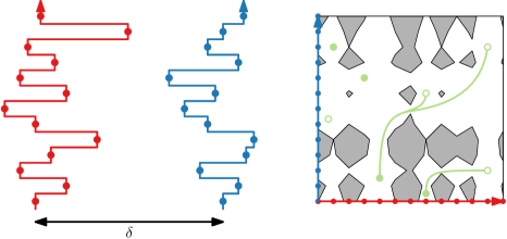
Figure 9: (left) A pair of separated, one-dimensional curves $R$ and $B$, drawn stretched vertically for clarity. (right) The free space $\mathcal{F}_{\delta}(R,B)$ corresponding to the matching, with a set of entrances (disks) and potential exits (circles). Some matchings between entrances and exits are drawn.

We assume that the points in $S$ and $E$ correspond to pairs of vertices of $R$ and $B$. This assumption can be met by introducing $\mathcal{O}(n+m)$ vertices, which does not increase our asymptotic running times. Additionally, we may assume that all vertices of $R$ and $B$ have unique values, for example by a symbolic perturbation.

The problem of propagating $\delta$-reachability information has already been studied by Bringmann and Künnemann [5]. In case $S$ lies on the left and bottom sides of the parameter space and $E$ lies on the top and right sides, they give an $\mathcal{O}((n+m)\log nm)$ time algorithm. We are interested in a more general case however, where $S$ and $E$ may lie anywhere in the parameter space. We make heavy use of the concept of prefix-minima to develop an algorithm for our more general setting that has the same running time as the one described by Bringmann and Künnemann [5]. Furthermore, our algorithm is able to actually compute a Fréchet matching between $R$ and $B$ in linear time (see Appendix˜A), while Bringmann and Künnemann require near-linear time for only the decision version.

Figure 10: (left) A prefix-minima matching, showing all pairs of prefix-minima matched in the matching. (right) The path in $\mathcal{F}_{\delta}(R,B)$ corresponding to the matching.

As mentioned above, we use prefix-minima extensively for our results in this section. Prefix-minima are those vertices that are closest to the separator $0$ among those points before them on the curves. In Section˜4.1 we prove that there exists a Fréchet matching that matches subcurves between consecutive prefix-minima to prefix-minima of the other curve (Lemma˜4.4), see Figure˜10 for an illustration. We call these matchings prefix-minima matchings. This matching will end in a bichromatic closest pair of points (Corollary˜4.3), and so we can compose the matching with a symmetric matching for the reversed curves.

In Section˜4.2 we introduce two forests of paths in $\mathcal{F}_{\delta}(R,B)$ starting at the points in $S$ that captures multiple prefix-minima matchings at once. It is based on horizontal-greedy and vertical-greedy matchings. We show that these forests have linear complexity and can be computed efficiently.

In Section˜4.3 we do not only go forward from points in $S$, but also backwards from points in $E$ using suffix-minima. Again we have horizontal-greedy and vertical-greedy versions. Intersections between the two prefix-minima paths and the two suffix minima paths show the existence of a $\delta$-free path of the corresponding points in $S$ and $E$, so the problem reduces to a bichromatic intersection algorithm.

4.1 Prefix-minima matchings

We investigate $\delta$-matchings based on prefix-minima of the curves. We call a vertex $R(i)$ a prefix-minimum of $R$ if $|R(i)|\leq|R(x)|$ for all $x\in[1,i]$. Prefix-minima of $B$ are defined symmetrically. Intuitively, prefix-minima are vertices that are closest to $0$ (the separator of $R$ and $B$) with respect to their corresponding prefix. Note that we may extend the definitions to points interior to edges as well, but the restriction to vertices is sufficient for our application.

The prefix-minima of a curve form a sequence of vertices that monotonically get closer to the separator. This leads to the following observation:

Lemma 4.1.

For any two prefix-minima $R(i)$ and $B(j)$, we have $d_{\mathrm{F}}(R[i,n],B[j,m])\leq d_{\mathrm{F}}(R,B)$.

Proof 4.2.

Consider a Fréchet matching $(f,g)$ between $R$ and $B$. It matches $R(i)$ to some point $B(y)$ and matches $B(j)$ to some point $R(x)$. Suppose without loss of generality that $y\geq j$; the other case is symmetric. The subcurve $R[x,i]$ is matched to the subcurve $B[j,y]$. By virtue of $R(i)$ being a prefix-minimum, it follows that $d_{\mathrm{F}}(R(i),B[j,y])\leq d_{\mathrm{F}}(R[x,i],B[j,y])\leq d_{\mathrm{F}}(R,B)$. Thus composing a matching between $R(i)$ and $B[j,y]$ with the matching between $R[i,n]$ and $B[y,m]$ induced by $(f,g)$ gives a matching with cost at most $d_{\mathrm{F}}(R,B)$.

The bichromatic closest pair of points $R(i^{*})$ and $B(j^{*})$ is formed by prefix-minima of the curves. (This pair of points is unique, by our general position assumption.) The points are also prefix-minima of the reversals of the curves. By using that the Fréchet distance between two curves is equal to the Fréchet distance between the two reversals of the curves, we obtain the following regarding matchings and bichromatic closest pairs of points:

Corollary 4.3.

There exists a Fréchet matching that matches $R(i^{*})$ to $B(j^{*})$.

Figure 11: (left) A pair of separated, one-dimensional curves $R$ and $B$, drawn stretched vertically for clarity. A prefix-minima matching, up to the last prefix-minima of the curves, is given in green. (right) The path in $\mathcal{F}_{\delta}(R,B)$ corresponding to the matching.

A $\delta$-matching $(f,g)$ is called a prefix-minima $\delta$-matching if for all $t\in[0,1]$ at least one of $R(f(t))$ and $B(g(t))$ is a prefix-minimum. Such a matching corresponds to a rectilinear path $\pi$ in $\mathcal{F}_{\delta}(R,B)$ where for each vertex $(i,j)$ of $\pi$, both $R(i)$ and $B(j)$ are prefix-minima. We call $\pi$ a prefix-minima $\delta$-matching as well. See Figure˜11 for an illustration. We show that there exists a prefix-minima Fréchet matching, up to any pair of prefix-minima:

Lemma 4.4.

Let $R(i)$ and $B(j)$ be prefix-minima of $R$ and $B$. There exists a prefix-minima Fréchet matching between $R[1,i]$ and $B[1,j]$.

Proof 4.5.

Let $(f,g)$ be a Fréchet matching between $R[1,i]$ and $B[1,j]$. If $i=1$ or $j=1$ then $(f,g)$ is naturally a prefix-minima Fréchet matching. We therefore assume $i\geq 2$ and $j\geq 2$, and consider the second prefix-minima $R(i^{\prime})$ and $B(j^{\prime})$ of $R$ and $B$ (the first being $R(1)$ and $B(1)$). Let $R(\hat{i})$ and $B(\hat{j})$ be the points (vertices) on $R[1,i^{\prime}]$ and $B[1,j^{\prime}]$ furthest from the separator $0$. Suppose $(f,g)$ matches $R(\hat{i})$ to a point $B(\hat{y})$, and matches a point $R(\hat{x})$ to $B(\hat{j})$. We assume that $\hat{x}\leq\hat{i}$; the other case, where $\hat{y}\leq\hat{j}$, is symmetric. We have $\hat{i}\leq i^{\prime}-1$, and hence $\hat{x}\leq i^{\prime}-1$. The subcurve $R[1,\hat{x}]$ contains no prefix-minima other than $R(1)$, so

$$|R(1)-B(y)|\leq|R(1)-B(\hat{j})|\leq|R(\hat{x})-B(\hat{j})|\leq d_{\mathrm{F}}(A[1,i],B[1,j])$$

for all $y\in[1,j^{\prime}]$. The unique matching (up to reparameterization) between $R(1)$ and $B[1,j^{\prime}]$ is therefore a prefix-minima matching with cost at most $d_{\mathrm{F}}(R[1,i],B[1,j])$. Lemma˜4.1 shows that $d_{\mathrm{F}}(R,B[j^{\prime},m])\leq d_{\mathrm{F}}(R[1,i],B[1,j])$, and so by inductively applying the above construction to $R$ and $B[j^{\prime},m]$, we obtain a prefix-minima Fréchet matching between $R[1,i]$ and $B[1,j]$.

4.2 Greedy paths in the free space

For the problem of propagating reachability from the set of entrances $S$ to the set of potential exits $E$, we wish to construct a set of canonical prefix-minima $\delta$-matchings in the free space from which we can deduce which points in $E$ are reachable. Naturally, we want to avoid constructing a path between every point in $S$ and every point in $E$. Therefore, we investigate certain classes of prefix-minima $\delta$-matchings that allows us to infer reachability information with just two paths per point in $S$ and two paths per point in $E$. Furthermore, these paths have a combined $\mathcal{O}(n+m)$ description complexity.

We first introduce one of the greedy matchings and prove a useful property. A horizontal-greedy $\delta$-matching $\pi_{\mathrm{hor}}$ is a prefix-minima $\delta$-matching starting at a point $s=(i,j)$ that satisfies the following property: Let $(i^{\prime},j^{\prime})$ be a point on $\pi_{\mathrm{hor}}$ with $R(i^{\prime})$ and $B(j^{\prime})$ prefix-minima of $R[i,n]$ and $B[j,m]$. If there exists a prefix-minimum $R(\hat{i})$ of $R[i,n]$ after $R(i^{\prime})$, and the horizontal line segment $[i^{\prime},\hat{i}]\times\{j^{\prime}\}$ lies in $\mathcal{F}_{\delta}(R,B)$, then either $\pi_{\mathrm{hor}}$ traverses this line segment, or $\pi_{\mathrm{hor}}$ terminates in $(i^{\prime},j^{\prime})$.

For an entrance $s\in S$, let $\pi_{\mathrm{hor}}(s)$ be the maximal horizontal-greedy $\delta$-matching. See Figure˜12 for an illustration. The path $\pi_{\mathrm{hor}}(s)$ serves as a canonical prefix-minima $\delta$-matching, in the sense that any point $t$ that is reachable from $s$ by a prefix-minima $\delta$-matching is reachable from a point on $\pi_{\mathrm{hor}}(s)$ through a single vertical segment:

Lemma 4.6.

Let $s\in S$ and let $t$ be a point that is reachable by a prefix-minima $\delta$-matching from $s$. A point $\hat{t}\in\pi_{\mathrm{hor}}(s)$ vertically below $t$ exists for which the segment $\overline{\hat{t}t}$ lies in $\mathcal{F}_{\delta}(R,B)$.

Proof 4.7.

Let $s=(i,j)$ and $t=(i^{\prime},j^{\prime})$. Consider a point $(\hat{i},\hat{j})\in\pi_{\mathrm{hor}}(s)$ with $\hat{i}\leq i^{\prime}$ and $\hat{j}\leq j^{\prime}$. By definition, $\pi_{\mathrm{hor}}(s)$ is a prefix-minima $\delta$-matching, so $R(\hat{i})$ and $B(\hat{j})$ are prefix-minima of $R[i,n]$ and $B[j,m]$, and hence of $R[i,i^{\prime}]$ and $B[j,j^{\prime}]$. By Lemma˜4.1, we have $d_{\mathrm{F}}(R[\hat{i},i^{\prime}],B[\hat{j},j^{\prime}])\leq d_{\mathrm{F}}(R[i,i^{\prime}],B[j,j^{\prime}])\leq\delta$. So there exists a $\delta$-matching from $(\hat{i},\hat{j})$ to $(i^{\prime},j^{\prime})$.

By the maximality of $\pi_{\mathrm{hor}}(s)$ and the property that $\pi_{\mathrm{hor}}(s)$ moves horizontal whenever possible, it follows that $\pi_{\mathrm{hor}}(s)$ reaches a point $(i^{\prime},\hat{j})$ with $\hat{j}\leq j^{\prime}$. The existence of a $\delta$-matching from $(i^{\prime},\hat{j})$ to $(i^{\prime},j^{\prime})$ follows from the above.

Figure 12: (left) For every vertex, its next prefix-minimum is depicted as its parent in the respective tree. (right) The horizontal-greedy $\delta$-matchings. Paths move monotonically to the right and up.

A single path $\pi_{\mathrm{hor}}(s)$ may have $\mathcal{O}(n+m)$ complexity. We would like to construct the paths for all entrances, but this would result in a combined complexity of $\mathcal{O}((n+m)^{2})$. However, due to the definition of the paths, if two paths $\pi_{\mathrm{hor}}(s)$ and $\pi_{\mathrm{hor}}(s^{\prime})$ have a point $(x,y)$ in common, then the paths are identical from $(x,y)$ onwards. Thus, rather than explicitly describing the paths, we instead describe their union.

The set $\bigcup_{s\in S}\pi_{\mathrm{hor}}(s)$ forms a geometric forest $\mathcal{T}_{\mathrm{hor}}(S)$ whose leaves are the points in $S$. We call $\mathcal{T}_{\mathrm{hor}}(S)$ the horizontal-greedy $\delta$-forest of $S$. See Figure˜12 for an illustration. In Sections˜4.2.1 and 4.2.2 we show that this forest has only $\mathcal{O}(n+m)$ complexity and give an $\mathcal{O}((n+m)\log nm)$-time construction algorithm.

4.2.1 Complexity of the forest

The horizontal-greedy forest $\mathcal{T}_{\mathrm{hor}}(S)$ is naturally equal to the union $\bigcup_{\pi\in\Pi}\pi$ of a set of $|S|$ horizontal-greedy $\delta$-matching $\Pi$ with interior-disjoint images that each start at a point in $S$. We analyse the complexity of $\mathcal{T}_{\mathrm{hor}}(S)$ by bounding the complexity of $\bigcup_{\pi\in\Pi}\pi$.

For the proofs, we introduce the notation $\mathcal{C}(\pi)$ to denote the set of integers $i\in\{1,\dots,n\}$ for which a path $\pi$ has a vertical edge on the line $\{i\}\times[1,m]$. We use the notation $\mathcal{R}(\pi)$ for representing the horizontal lines containing a horizontal edge of $\pi$. The number of edges $\pi$ has is $|\mathcal{C}(\pi)|+|\mathcal{R}(\pi)|$.

Lemma 4.8.

For any two interior-disjoint horizontal-greedy $\delta$-matching $\pi$ and $\pi^{\prime}$, we have $|\mathcal{C}(\pi)\cap\mathcal{C}(\pi^{\prime})|\leq 1$ or $|\mathcal{R}(\pi)\cap\mathcal{R}(\pi^{\prime})|\leq 1$.

Proof 4.9.

If $\mathcal{C}(\pi)\cap\mathcal{C}(\pi^{\prime})=\emptyset$ or $\mathcal{R}(\pi)\cap\mathcal{R}(\pi^{\prime})=\emptyset$, the statement trivially holds. We therefore assume that the paths have colinear horizontal edges and colinear vertical edges.

We assume without loss of generality that $\pi$ lies above $\pi^{\prime}$, so $\pi$ does not have any points that lie vertically below points on $\pi^{\prime}$. Let $e_{\mathrm{hor}}=[i_{1},i_{2}]\times\{j\}$ and $e_{\mathrm{ver}}=\{i\}\times[j_{1},j_{2}]$ be the first edges of $\pi$ that are colinear with a horizontal, respectively vertical, edge of $\pi^{\prime}$. Let $e^{\prime}_{\mathrm{hor}}=[i^{\prime}_{1},i^{\prime}_{2}]\times\{j\}$ and $e^{\prime}_{\mathrm{ver}}=\{i\}\times[j^{\prime}_{1},j^{\prime}_{2}]$ be the edges of $\pi^{\prime}$ that are colinear with $e_{\mathrm{hor}}$ and $e_{\mathrm{ver}}$, respectively. We distinguish between the order of $e_{\mathrm{hor}}$ and $e_{\mathrm{ver}}$ along $\pi$.

First suppose $e_{\mathrm{hor}}$ comes before $e_{\mathrm{ver}}$ along $\pi$. Let $e^{\prime}_{\mathrm{ver}}=\{i\}\times[j^{\prime}_{1},j^{\prime}_{2}]$ be the edge of $\pi^{\prime}$ that is colinear with $e_{\mathrm{ver}}$. This edge lies vertically below $e_{\mathrm{ver}}$, so $j^{\prime}_{2}\leq j_{1}$. If $\pi^{\prime}$ terminates at $(i,j^{\prime}_{2})$, then $\mathcal{C}(\pi)\cap\mathcal{C}(\pi^{\prime})=\{i\}$ and the claim holds. Next we show that $\pi^{\prime}$ must terminate at $(i,j^{\prime}_{2})$.

Suppose for sake of contradiction that $\pi^{\prime}$ has a horizontal edge $[i,i^{\prime}]\times\{j^{\prime}\}$. We have $j^{\prime}\leq j_{1}$. By virtue of $\pi^{\prime}$ being a prefix-minima $\delta$-matching, we obtain that $B(j^{\prime})$ is a prefix-minimum of $B[y,j^{\prime}]$ for every point $(x,y)$ on $\pi^{\prime}$. In particular, since $\pi^{\prime}$ has a horizontal edge that is colinear with $e_{\mathrm{hor}}$, we have that $B(j^{\prime})$ is a prefix-minimum of $B[j,j^{\prime}]$, and thus of $B[j,j^{\prime}_{1}]$. Additionally, by virtue of $\pi$ being a prefix-minima $\delta$-matching, we obtain that $B(j^{\prime}_{1})$ is a prefix-minimum of $B[j,j^{\prime}_{1}]$. Hence $|B(j^{\prime}_{1})|\leq|B(j^{\prime})|$, which shows that the horizontal line segment $[i,i^{\prime}]\times\{j^{\prime}_{1}\}$ lies in $\mathcal{F}_{\delta}(R,B)$. However, this means that $\pi$ cannot have $e_{\mathrm{ver}}$ as an edge, as $\pi$ is horizontal-greedy. This gives a contradiction.

The above proves the statement when $e_{\mathrm{hor}}$ comes before $e_{\mathrm{ver}}$ along $\pi$. Next we prove the statement when $e_{\mathrm{hor}}$ comes after $e_{\mathrm{ver}}$ along $\pi$. By virtue of $\pi^{\prime}$ being a prefix-minimum $\delta$-matching, we have that $B(j)$ is a prefix-minimum of $B[y,j]$ for every point $(x,y)$ on $\pi^{\prime}$. It follows that for all points $(x,y)$ on $\pi^{\prime}$ with $x\in[i,i^{\prime}_{1}]$, we have $|R(x)-B(j)|\leq|R(x)-B(y)|\leq\delta$. Hence the horizontal line segment $[\max\{i_{1},i\},i^{\prime}_{1}]\times\{j\}$ lies in $\mathcal{F}_{\delta}(R,B)$. Because $e_{\mathrm{hor}}$ comes after $e_{\mathrm{ver}}$, we further have $i_{1}\geq i$. Thus, the horizontal-greedy $\delta$-matching $\pi$ must fully contain the horizontal segment $[i_{1},i^{\prime}_{1}]\times\{j\}$, or terminate in a point on this segment. If $\pi$ reaches the point $(i^{\prime}_{1},j)$, then either $\pi$ or $\pi^{\prime}$ terminates in this point, since the two paths are interior-disjoint. Hence we have $\mathcal{R}(\pi)\cap\mathcal{R}(\pi^{\prime})=\{j\}$, proving the statement.

Lemma 4.10.

The forest $\mathcal{T}_{\mathrm{hor}}(S)$ has $\mathcal{O}(n+m)$ vertices.

Proof 4.11.

We bound the number of edges of $\mathcal{T}_{\mathrm{hor}}(S)$. The forest has at most $|S|=\mathcal{O}(n+m)$ connected components, and since each connected component is a tree, the number of vertices of such a component is exactly one greater than the number of edges. Thus the number of vertices is at most $\mathcal{O}(n+m)$ greater than the number of edges.

There exists a collection of $|S|$ horizontal-greedy $\delta$-matchings $\Pi$ that all start at points in $S$ and have interior-disjoint images, for which $\mathcal{T}_{\mathrm{hor}}(S)=\bigcup_{\pi\in\Pi}\pi$. Let $\pi_{1},\dots,\pi_{|\Pi|}$ be the $\mathcal{O}(n+m)$ paths in $\Pi$, in arbitrary order. We write $c_{i}=|\mathcal{C}(\pi_{i})|$, $r_{i}=|\mathcal{R}(\pi_{i})|$ and $k_{i}=|\mathcal{C}(\pi_{i})|+|\mathcal{R}(\pi_{i})|$, and proceed to bound $\sum_{i}k_{i}$. This quantity is equal to the number of edges of $\mathcal{T}_{\mathrm{hor}}(S)$.

By Lemma˜4.8, for all pairs of paths $\pi_{i}$ and $\pi_{j}$ we have that $|\mathcal{C}(\pi_{i})\cap\mathcal{C}(\pi_{j})|\leq 1$ or $|\mathcal{R}(\pi_{i})\cap\mathcal{R}(\pi_{j})|\leq 1$. Let $x_{i,j}\in\{0,1\}$ be an indicator variable that is set to $1$ if $|\mathcal{C}(\pi_{i})\cap\mathcal{C}(\pi_{j})|\leq 1$ and $0$ if $|\mathcal{R}(\pi_{i})\cap\mathcal{R}(\pi_{j})|\leq 1$ (with an arbitrary value if both hold). We then get the following bounds on $c_{i}$ and $r_{i}$:

$$c_{i}\leq n-\sum_{j\neq i}x_{i,j}\cdot(c_{j}-1)\quad\text{and}\quad r_{i}\leq m-\sum_{j\neq i}(1-x_{i,j})\cdot(r_{j}-1).$$

We naturally have that $|c_{j}-r_{j}|\leq 1$ for all paths $\pi_{j}$, and so $k_{j}=c_{j}+r_{j}\leq 2\min\{c_{j},r_{j}\}+1$. Hence we obtain that

$$c_{i}\leq n-\sum_{j\neq i}x_{i,j}\cdot\left(\frac{k_{j}-1}{2}-1\right)\quad\text{and}\quad r_{i}\leq m-\sum_{j\neq i}(1-x_{i,j})\cdot\left(\frac{k_{j}-1}{2}-1\right),$$

from which it follows that

$$k_{i}\leq n+m-\sum_{j\neq i}\left(\frac{k_{j}-1}{2}-1\right)=\mathcal{O}(n+m)-\frac{1}{2}\sum_{j\neq i}k_{j}.$$

We proceed to bound the quantity $\sum_{\pi\in\Pi}(|\mathcal{C}(\pi)|+|\mathcal{R}(\pi)|)=\sum_{i}k_{i}$, which bounds the total number of edges of the paths in $\Pi$, and thus the number of edges of $\mathcal{T}_{\mathrm{hor}}(S)$:

$$\sum_{i=1}^{|\Pi|}k_{i} =\sum_{i=3}^{|\Pi|}k_{i}+k_{1}+k_{2}$$

$$\leq\sum_{i=3}^{|\Pi|}k_{i}+\mathcal{O}(n+m)-\frac{1}{2}\sum_{j\neq 1}k_{j}-\frac{1}{2}\sum_{j\neq 2}k_{j}$$

$$=\sum_{i=3}^{|\Pi|}k_{i}+\mathcal{O}(n+m)-\frac{1}{2}(k_{1}+k_{2})-\sum_{i=3}^{|\Pi|}k_{i}$$

$$=\mathcal{O}(n+m).$$

4.2.2 Constructing the forest

We turn to constructing the forest $\mathcal{T}_{\mathrm{hor}}(S)$. For this task, we require a data structure that determines, for a vertex of a maximal horizontal-greedy $\delta$-matching, where its next vertex lies. We make use of two auxiliary data structures that store one-dimensional curves $A$. The first determines, for a given point $A(x)$ and threshold value $U$, the maximum subcurve $A[x,x^{\prime}]$ on which no point’s value exceeds $U$.

Lemma 4.12.

Let $A$ be a one-dimensional curve with $k$ vertices. In $\mathcal{O}(k\log k)$ time, we can construct a data structure of $\mathcal{O}(k)$ size, such that given a point $A(x)$ and a threshold value $U\geq A(x)$, the last point $A(x^{\prime})$ with $\max_{\hat{x}\in[x,x^{\prime}]}A(\hat{x})\leq U$ can be reported in $\mathcal{O}(\log k)$ time.

Proof 4.13.

We use a persistent red-black tree, of which we first describe the ephemeral variant. Let $T_{i}$ be a red-black tree storing the vertices of $A[i,k]$ in its leaves, based on their order along $A$. The tree has $\mathcal{O}(\log k)$ height. We augment every node of $T_{i}$ with the last vertex stored in its subtree that has the minimum value. To build the tree $T_{i-1}$ from $T_{i}$, we insert $A(i-1)$ into $T_{i}$ by letting it be the leftmost leaf. This insertion operation costs $\mathcal{O}(\log k)$ time, but only at most two “rotations” are used to rebalance the tree [17]. Each rotation affects $\mathcal{O}(1)$ nodes of the tree, and the subtrees containing these nodes require updating their associated vertex. There are $\mathcal{O}(\log k)$ such subtrees and updating them takes $\mathcal{O}(\log k)$ time in total. Inserting a point therefore takes $\mathcal{O}(\log k)$ time. To keep representations of all trees $T_{i}$ in memory, we use persistence [13]. With the techniques of [13] to make the data structure persistent, we may access any tree $T_{i}$ in $\mathcal{O}(\log k)$ time. The trees all have $\mathcal{O}(\log k)$ height. The time taken to construct all trees is $\mathcal{O}(k\log k)$.

Consider a query with a point $A(x)$ and value $U\in\mathbb{R}$. Let $e=A[i,i+1]$ be the edge of $A$ containing $A(x)$, picking $i=x$ if $A(x)$ is a vertex with two incident edges. We first compute the last point on $e$ whose value does not exceed the threshold $U$. If this point is not the second endpoint $A(i+1)$ of $e$, then we report this point as the answer to the query. Otherwise, we continue to report the last vertex $A(i^{\prime})$ after $A(i+1)$ for which $\max_{\hat{x}\in[x,x^{\prime}]}A(\hat{x})\leq U$. The answer to the query is on the edge $A[i^{\prime},i^{\prime}+1]$.

We first access $T_{i}$. We then traverse $T_{i}$ from root to leaf in the following manner: Suppose we are in a node $\mu$ and let its left subtree store the vertices of $A[i_{1},i_{2}]$ and its right subtree the vertices of $A[i_{2}+1,i_{3}]$. If the left child of $\mu$ is augmented with a value greater than $U$, then $A(\hat{i})>U$ for some $\hat{i}\in[i_{1},i_{2}]$. In this case, we continue the search by going into the left child of $\mu$. Otherwise, we remember $i_{2}$ as a candidate for $i^{\prime}$ and continue the search by going into the right child of $\mu$. In the end, we have $\mathcal{O}(\log k)$ candidates for $i^{\prime}$, and we pick the last index.

Given $i^{\prime}$, we report the last point on the edge $A[i^{\prime},i^{\prime}+1]$ (or $A(i^{\prime})$ itself if $i^{\prime}=k$) whose value does not exceed $U$ as the answer to the query. We find $i^{\prime}$ in $\mathcal{O}(\log k)$ time, giving a query time of $\mathcal{O}(\log k)$.

We also make use of a range minimum query data structure. A range minimum query on a subcurve $A[x,x^{\prime}]$ reports the minimum value of the subcurve. This value is either $A(x)$, $A(x^{\prime})$, or the minimum value of a vertex of $A[\lceil x\rceil,\lfloor x^{\prime}\rfloor]$. Hence range minimum queries can be answered in $\mathcal{O}(1)$ time after $\mathcal{O}(k)$ time preprocessing (see e.g. [15]). However, we give an alternative data structure with $\mathcal{O}(\log k)$ query time. Our data structure additionally allows us to query a given range for the first value below a given threshold. This latter type of query is also needed for the construction of $\mathcal{T}_{\mathrm{hor}}(S)$. The data structure has the added benefit of working in the pointer-machine model of computation.

Lemma 4.14.

Let $A$ be a one-dimensional curve with $k$ vertices. In $\mathcal{O}(k)$ time, we can construct a data structure of $\mathcal{O}(k)$ size, such that the minimum values of a query subcurve $A[x,x^{\prime}]$ can be reported in $\mathcal{O}(\log k)$ time. Additionally, given a threshold value $U\in\mathbb{R}$, the first and last points $A(x^{*})$ on $A[x,x^{\prime}]$ with $A(x^{*})\leq U$ (if they exist) can be reported in $\mathcal{O}(\log k)$ time.

Proof 4.15.

We show how to preprocess $A$ for querying the minimum value of a subcurve $A[x,x^{\prime}]$, as well as the first point $A(x^{*})$ on $A[x,x^{\prime}]$ with $A(x^{*})\leq U$ for a query threshold value $U\in\mathbb{R}$. Preprocessing and querying for the other property is symmetric.

We store the vertices of $A$ in the leaves of a balanced binary search tree $T$, based on their order along $A$. We augment each node of $T$ with the minimum value of the vertices stored in its subtree. Constructing a balanced binary search tree $T$ on $A$ takes $\mathcal{O}(k)$ time, since the vertices are pre-sorted. Augmenting the nodes takes $\mathcal{O}(k)$ time in total as well, through a bottom-up traversal of $T$.

Consider a query with a subcurve $A[x,x^{\prime}]$. The minimum value of a point on this subcurve is attained by either $A(x)$, $A(x^{\prime})$, or a vertex of $A[i,i^{\prime}]$ with $i=\lceil x\rceil$ and $i^{\prime}=\lfloor x^{\prime}\rfloor$. We query $T$ for the minimum value of a vertex of $A[i,i^{\prime}]$. For this, we identify $\mathcal{O}(\log k)$ nodes whose subtrees combined store exactly the vertices of $A[i,i^{\prime}]$. These nodes store a combined $\mathcal{O}(\log k)$ candidate values for the minimum, and we identify the minimum in $\mathcal{O}(\log k)$ time. Comparing this minimum to $A(x)$ and $A(x^{\prime})$ gives the minimum of $A[x,x^{\prime}]$.

Given a threshold value $U\in\mathbb{R}$, the first point $A(x^{*})$ of $A[x,x^{\prime}]$ with $A(x^{*})\leq U$ can be reported similarly to the minimum of the subcurve. If $x$ and $x^{\prime}$ lie on the same edge of $A$, we report the answer in constant time. Next suppose $i=\lceil x\rceil\leq\lfloor x^{\prime}\rfloor=i^{\prime}$.

We start by reporting the first vertex $A(i^{*})$ of $A[i,i^{\prime}]$ with $A(i^{*})\leq U$ (if it exists). For this, we again identify $\mathcal{O}(\log k)$ nodes whose subtrees combined store exactly the vertices of $A[i,i^{\prime}]$. Each node stores the minimum value of the vertices stored in its subtree, and so the leftmost node $\mu$ storing a value below $U$ contains $A(i^{*})$. (If no such node $\mu$ exists, then $A(i^{*})$ does not exist.) To get to $A(i^{*})$, we traverse the subtree of $\mu$ to a leaf, by always going into the left subtree if it stores a value below $U$. Identifying $\mu$ takes $\mathcal{O}(\log k)$ time, and traversing its subtree down to $A(i^{*})$ takes an additional $\mathcal{O}(\log k)$ time.

Given $A(i^{*})$, the point $A(x^{*})$ lies on the edge $A[i^{*}-1,i^{*}]$ and we compute it in $\mathcal{O}(1)$ time. If $i^{*}$ does not exist, then $A(x^{*})$ is equal to either $A(x)$ or $A(x^{\prime})$, and we report $A(x^{*})$ in $\mathcal{O}(1)$ time.

Next we give two data structures, one that determines how far we may extend a horizontal-greedy $\delta$-matching horizontally, and one that determines how far we may extend it vertically.

Horizontal movement.

We preprocess $R$ into the data structures of Lemmas˜4.12 and 4.14, taking $\mathcal{O}(n\log n)$ time. To determine the maximum horizontal movement from a given vertex $(i,j)$ on a horizontal-greedy $\delta$-matching $\pi$, we first report the last vertex $R(i^{\prime})$ after $R(i)$ for which $\max_{x\in[i,i^{\prime}]}|R(x)|\leq\delta-|B(j)|$. Since $R$ lies completely left of $0$, we have $\max_{x\in[i,i^{\prime}]}|R(x)|=\min_{x\in[i,i^{\prime}]}R(x)$, and so this vertex can be reported in $\mathcal{O}(\log n)$ time with the data structure of Lemma˜4.12.

Next we report the last prefix-minimum $R(i^{*})$ of $R[i,i^{\prime}]$. The path $\pi$ may move horizontally from $(i,j)$ to $(i^{*},j)$ and not further. Observe that $R(i^{*})$ is the last vertex of $R[i,i^{\prime}]$ with $|R(i^{*})|\leq\min_{x\in[i,i^{\prime}]}|R(x)|$. We report the value of $\min_{x\in[i,i^{\prime}]}|R(x)|$ in $\mathcal{O}(\log n)$ time with the data structure of Lemma˜4.14. The vertex $R(i^{*})$ of $R[i,i^{\prime}]$ can then be reported in $\mathcal{O}(\log n)$ additional time with the same data structure.

Lemma 4.16.

In $\mathcal{O}(n\log n)$ time, we can construct a data structure of $\mathcal{O}(n)$ size, such that given a vertex $(i,j)$ of a horizontal-greedy $\delta$-matching $\pi$, the maximal horizontal line segment that $\pi$ may use as an edge from $(i,j)$ can be reported in $\mathcal{O}(\log n)$ time.

Vertical movement.

To determine the maximum vertical movement from a given vertex $(i,j)$ on a horizontal-greedy $\delta$-matching $\pi$, we need to determine the first prefix-minimum $B(j^{\prime})$ of $B[j,j^{\prime}]$ for which a horizontal-greedy $\delta$-matching needs to move horizontally from $(i,j^{\prime})$. For this, we make use of the following data structure that determines the second prefix-minimum $R(i^{*})$ of $R[i,n]$:

Lemma 4.17.

In $\mathcal{O}(n)$ time, we can construct a data structure of $\mathcal{O}(n)$ size, such that given a vertex $R(i)$, the second prefix-minimum of $R[i,n]$ (if it exists) can be reported in $\mathcal{O}(1)$ time.

Proof 4.18.

We use the algorithm of Berkman et al. [2] to compute, for every vertex $R(i)$ of $R$, the first vertex $R(i^{*})$ after $R(i)$ with $|R(i^{*})|\leq|R(i)|$ (if it exists). Naturally, $R(i^{*})$ is the second prefix-minimum of $R(i)$. Their algorithm takes $\mathcal{O}(n)$ time. Annotating the vertices of $R$ with their respective second prefix-minima gives a $\mathcal{O}(n)$-size data structure with $\mathcal{O}(1)$ query time.

The first prefix-minimum $B(j^{\prime})$ of $B[j,j^{\prime}]$ for which a horizontal-greedy $\delta$-matching needs to move horizontally from $(i,j^{\prime})$, is the first prefix-minimum with $d_{\mathrm{F}}(R[i,i^{*}],B(j^{\prime}))\leq\delta$. Observe that $B(j^{\prime})$ is not only the first prefix-minimum of $B[j,m]$ with $d_{\mathrm{F}}(R[i,i^{*}],B(j^{\prime}))\leq\delta$, it is also the first vertex of $B[j,m]$ with this property.

We preprocess $B$ into the data structures of Lemmas˜4.12 and 4.14, taking $\mathcal{O}(m\log m)$ time. We additionally preprocess $A$ into the data structure of Lemma˜4.14, taking $\mathcal{O}(n\log n)$ time.

We first compute $\max_{x\in[i,i^{*}]}|R(x)|=\min_{x\in[i,i^{*}]}R(x)$ with the data structure of Lemma˜4.14, taking $\mathcal{O}(\log n)$ time. We then report $B(j^{\prime})$ as the first vertex of $B[j,m]$ with $|B(j^{\prime})|\leq\delta-\max_{x\in[i,i^{*}]}|R(x)|$. This takes $\mathcal{O}(\log m)$ time.

To determine the maximum vertical movement of $\pi$, we need to compute the maximum vertical line segment $\{i\}\times[j,j^{*}]\subseteq\mathcal{F}_{\delta}(R,B)$ for which $B(j^{*})$ is a prefix-minimum of $B[j,j^{\prime}]$. We query the data structure of Lemma˜4.12 for the last vertex $B(\hat{j})$ for which $\max_{y\in[j,\hat{j}]}|B(y)|\leq\delta-|R(i)|$. This takes $\mathcal{O}(\log m)$ time. The vertex $B(j^{*})$ is then the last prefix-minimum of $B[j,\hat{j}]$, which we report in $\mathcal{O}(\log m)$ time with the data structure of Lemma˜4.14, by first computing the minimum value of $B[j,\hat{j}]$ and then the last vertex that attains this value.

Lemma 4.19.

In $\mathcal{O}((n+m)\log nm)$ time, we can construct a data structure of $\mathcal{O}(n+m)$ size, such that given a vertex $(i,j)$ of a horizontal-greedy $\delta$-matching $\pi$, the maximal vertical line segment that $\pi$ may use as an edge from $(i,j)$ can be reported in $\mathcal{O}(\log nm)$ time.

Completing the construction.

We proceed to iteratively construct the forest $\mathcal{T}_{\mathrm{hor}}(S)$. Let $S^{\prime}\subseteq S$ and suppose we have the forest $\mathcal{T}_{\mathrm{hor}}(S^{\prime})$. Initially, $\mathcal{T}_{\mathrm{hor}}(\emptyset)$ is the empty forest. We show how to construct $\mathcal{T}_{\mathrm{hor}}(S^{\prime}\cup\{s\})$ for a point $s\in S\setminus S^{\prime}$.

We assume $\mathcal{T}_{\mathrm{hor}}(S^{\prime})$ is represented as a geometric graph. Further, we assume that the $\mathcal{O}(n+m)$ vertices of $\mathcal{T}_{\mathrm{hor}}(S^{\prime})$ are stored in a red-black tree, based on the lexicographical ordering of the endpoints. This allows us to query whether a given point is a vertex of $\mathcal{T}_{\mathrm{hor}}(S^{\prime})$ in $\mathcal{O}(\log nm)$ time, and also allows us to insert new vertices in $\mathcal{O}(\log nm)$ time each.

We use the data structures of Lemmas˜4.16 and 4.19. These allow us compute the edge of $\pi_{\mathrm{hor}}(s)$ after a given vertex in $\mathcal{O}(\log nm)$ time. The preprocessing for the data structures is $\mathcal{O}((n+m)\log nm)$.

We construct the prefix $\pi$ of $\pi_{\mathrm{hor}}(s)$ up to the first vertex of $\pi_{\mathrm{hor}}(s)$ that is a vertex of $\mathcal{T}_{\mathrm{hor}}(S^{\prime})$ (or until the last vertex of $\pi_{\mathrm{hor}}(s)$ if no such vertex exists). This takes $\mathcal{O}(|\pi|\log nm)$ time, where $|\pi|$ is the number of vertices of $\pi$. Recall that if two maximal horizontal-greedy $\delta$-matchings $\pi_{\mathrm{hor}}(s)$ and $\pi_{\mathrm{hor}}(s^{\prime})$ have a point $(x,y)$ in common, then the paths are identical from $(x,y)$ onwards. Thus the remainder of $\pi_{\mathrm{hor}}(s)$ is a path in $\mathcal{T}_{\mathrm{hor}}(S^{\prime})$.

We add all vertices and edges of $\pi$, except the last two vertices $p$ and $q$ and the last edge $e=\overline{pq}$, to $\mathcal{T}_{\mathrm{hor}}(S^{\prime})$. If $\mathcal{T}_{\mathrm{hor}}(S^{\prime})$ does not have a vertex at point $q$ already, then $q$ does not lie anywhere on $\mathcal{T}_{\mathrm{hor}}(S^{\prime})$, not even interior to an edge. Hence $\pi$ is completely disjoint from $\mathcal{T}_{\mathrm{hor}}(S^{\prime})$, and we add $p$ and $q$ as vertices to the forest, and $e$ as an edge. If $\mathcal{T}_{\mathrm{hor}}(S^{\prime})$ does have a vertex $\mu$ at point $q$, then the edge $e$ may overlap with an edge of $\mathcal{T}_{\mathrm{hor}}(S^{\prime})$. In this case, we retrieve the edge $e_{\mu}$ of $\mathcal{T}_{\mathrm{hor}}(S^{\prime})$ that overlaps with $e$ (if it exists), by identifying the edges incident to $\mu$. If $p$ lies on $e_{\mu}$, we subdivide $e_{\mu}$ by adding a vertex at $p$. If $p$ does not lie on $e_{\mu}$, then the endpoint $q_{\mu}$ of $e_{\mu}$ other than $q$ lies on the interior of $e$. We add an edge from $p$ to $q_{\mu}$.

The above construction updates $\mathcal{T}_{\mathrm{hor}}(S^{\prime})$ into the forest $\mathcal{T}_{\mathrm{hor}}(S^{\prime}\cup\{s\})$ in $\mathcal{O}(|\pi|\log nm)$ time. Inserting all $\mathcal{O}(|\pi|)$ newly added vertices into the red-black tree takes an additional $\mathcal{O}(|\pi|\log nm)$ time. It follows from the combined $\mathcal{O}(n+m)$ complexity of $\mathcal{T}_{\mathrm{hor}}(S)$ that constructing $\mathcal{T}_{\mathrm{hor}}(S)$ in this manner takes $\mathcal{O}((n+m)\log nm)$ time.

Lemma 4.20.

We can construct a geometric graph for $\mathcal{T}_{\mathrm{hor}}(S)$ in $\mathcal{O}((n+m)\log nm)$ time.

4.3 Propagating reachability

Next we give an algorithm for propagating reachability information from the set of entrances $S$ to the set of potential exits $E$.

For the algorithm, we consider one more greedy $\delta$-matching. This matching requires a symmetric definition to prefix-minima, namely suffix-minima. These are the vertices closest to $0$ compared to the suffix of the curve after the vertex. The maximal reverse vertical-greedy $\delta$-matching $\reflectbox{$\vec{\reflectbox{\!$\pi$}}$}_{\mathrm{ver}}(t)$ is symmetric in definition to the maximal horizontal-greedy $\delta$-matching. It is a $\delta$-matching that moves backwards, to the left and down, starting at $t$. Its vertices corresponding to suffix-minima of the curves (see Figure˜13), and it prioritizes vertical movement over horizontal movement.

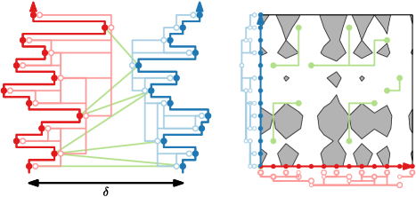
Figure 13: (left) For every vertex, its previous suffix-minimum is shown as its parent in the tree. (right) The reverse vertical-greedy $\delta$-matchings. Paths move monotonically to the left and down.

Consider a point $s=(i,j)\in S$ and let $t=(i^{\prime},j^{\prime})\in E$ be $\delta$-reachable from $s$. Let $R(i^{*})$ and $B(j^{*})$ form a bichromatic closest pair of $R$ and $B$. Note that these points are unique, by our general position assumption. We proved in Corollary˜4.3 that $(i^{*},j^{*})$ is $\delta$-reachable from $s$, and that $t$ is $\delta$-reachable from $(i^{*},j^{*})$.

From Lemma˜4.6 we have that $\pi_{\mathrm{hor}}(s)$ has points vertically below $(i^{*},j^{*})$, and the vertical segment between $\pi_{\mathrm{hor}}(s)$ and $(i^{*},j^{*})$ lies in $\mathcal{F}_{\delta}(R,B)$. We extend the property to somewhat predict the movement of $\pi_{\mathrm{hor}}(s)$ near $t$:

Lemma 4.21.

Either $\pi_{\mathrm{hor}}(s)$ terminates in $(i^{*},j^{*})$, or it contains a point vertically below $t$ or horizontally left of $t$.

Proof 4.22.

From Lemma˜4.6 we obtain that there exists a point $(i^{*},\hat{j})$ on $\pi_{\mathrm{hor}}(s)$ that lies vertically below $(i^{*},j^{*})$. Moreover, the vertical line segment $\{i^{*}\}\times[\hat{j},j^{*}]$ lies in $\mathcal{F}_{\delta}(R,B)$. Because $R(i^{*})$ and $B(j^{*})$ form the unique bichromatic closest pair of $R[i,i^{\prime}]$ and $B[j,j^{\prime}]$, we have that $R(i^{*})$ and $B(j^{*})$ are the last prefix-minima of $R[i,i^{\prime}]$ and $B[j,j^{\prime}]$. Hence $\pi_{\mathrm{hor}}(s)$ has no vertex in the vertical slab $[i^{*}+1,i^{\prime}]\times[1,m]$. Symmetrically, $\pi_{\mathrm{hor}}(s)$ has no vertex inin the horizontal slab $[1,n]\times[j^{*}+1,j^{\prime}]$. Maximality of $\pi_{\mathrm{hor}}(s)$ therefore implies that $\pi_{\mathrm{hor}}(s)$ either moves horizontally from $(i^{*},\hat{j})$ past $(i^{\prime},\hat{j})$, or $\pi_{\mathrm{hor}}(s)$ moves vertically from $(i^{*},\hat{j})$ to $(i^{*},j^{*})$, where it either terminates or moves further upwards past $(i^{*},j^{\prime})$.

Using symmetry, Lemmas˜4.6 and 4.21 imply that we have the following regarding $\pi_{\mathrm{hor}}(s)$ and $\reflectbox{$\vec{\reflectbox{\!$\pi$}}$}_{\mathrm{ver}}(t)$:

• $\pi_{\mathrm{hor}}(s)$ has a point vertically below $(i^{*},j^{*})$, and the vertical segment between $\pi_{\mathrm{hor}}(s)$ and $(i^{*},j^{*})$ lies in $\mathcal{F}_{\delta}(R,B)$.

• $\reflectbox{$\vec{\reflectbox{\!$\pi$}}$}_{\mathrm{ver}}(t)$ has a point horizontally right of $(i^{*},j^{*})$, and the horizontal segment between $\reflectbox{$\vec{\reflectbox{\!$\pi$}}$}_{\mathrm{ver}}(t)$ and $(i^{*},j^{*})$ lies in $\mathcal{F}_{\delta}(R,B)$.

• $\pi_{\mathrm{hor}}(s)$ (resp. $\reflectbox{$\vec{\reflectbox{\!$\pi$}}$}_{\mathrm{ver}}(t)$) either terminates in $(i^{*},j^{*})$, or contains a point vertically below $t$ (resp. horizontally right of $s$).

These properties imply a useful result regarding the extensions of the paths. We extend the paths in the following manner. Let $\pi^{+}_{\mathrm{hor}}(s)$ be the path obtained by extending $\pi_{\mathrm{hor}}(s)$ with the maximum horizontal line segment in $\mathcal{F}_{\delta}(R,B)$ whose left endpoint is the end of $\pi_{\mathrm{hor}}(s)$. Define $\reflectbox{$\vec{\reflectbox{\!$\pi$}}$}^{+}_{\mathrm{ver}}(t)$ analogously, by extending $\reflectbox{$\vec{\reflectbox{\!$\pi$}}$}_{\mathrm{ver}}(t)$ with a vertical segment. By the properties from Lemma˜4.6, we now have that $\pi^{+}_{\mathrm{hor}}(s)$ must intersect $\reflectbox{$\vec{\reflectbox{\!$\pi$}}$}^{+}_{\mathrm{ver}}(t)$. Furthermore, if $\pi^{+}_{\mathrm{hor}}(s)$ intersects $\reflectbox{$\vec{\reflectbox{\!$\pi$}}$}^{+}_{\mathrm{ver}}(t^{\prime})$ for some potential exit $t^{\prime}\in E$, then the bimonotonicity of the paths implies that $t^{\prime}$ is $\delta$-reachable from $s$.

Lemma 4.23.

Let $s\in S$ and $t\in E$. The point $t$ is $\delta$-reachable from $s$ if and only if $\pi^{+}_{\mathrm{hor}}(s)$ intersects $\reflectbox{$\vec{\reflectbox{\!$\pi$}}$}^{+}_{\mathrm{ver}}(t^{\prime})$.

Recall that $\mathcal{T}_{\mathrm{hor}}(S)$ represents all paths $\pi_{\mathrm{hor}}(s)$, and that we can construct $\mathcal{T}_{\mathrm{hor}}(S)$ as a geometric graph of complexity $\mathcal{O}(n+m)$ in $\mathcal{O}((n+m)\log nm)$ time (see Lemmas˜4.10 and 4.20). We augment $\mathcal{T}_{\mathrm{hor}}(S)$ to represent all paths $\pi^{+}_{\mathrm{hor}}(s)$. For this, we take each root vertex $p$ and compute the maximal horizontal segment $\overline{pq}\subseteq\mathcal{F}_{\delta}(R,B)$ that has $p$ as its left endpoint. We compute this segment in $\mathcal{O}(\log n)$ time after $\mathcal{O}(n\log n)$ time preprocessing (see Lemma˜4.12). We then add $q$ as a vertex to $\mathcal{T}_{\mathrm{hor}}(S)$, and add an edge from $p$ to $q$.

Let $\mathcal{T}^{+}_{\mathrm{hor}}(S)$ be the augmented graph. We define the graph $\reflectbox{$\vec{\reflectbox{\!$\mathcal{T}$}}$}^{+}_{\mathrm{ver}}(E)$ analogously. The two graphs have a combined complexity of $\mathcal{O}(n+m)$ and can be constructed in $\mathcal{O}((n+m)\log nm)$ time. Our algorithm computes the edges of $\reflectbox{$\vec{\reflectbox{\!$\mathcal{T}$}}$}^{+}_{\mathrm{ver}}(E)$ that intersect an edge of $\mathcal{T}^{+}_{\mathrm{hor}}(S)$. We do so with a standard sweepline algorithm:

Lemma 4.24.

Let $L_{R}$ and $L_{B}$ be two sets of $n$ “red,” respectively $m$ “blue,” horizontal and vertical line segments in $\mathbb{R}^{2}$. We can report all segments that intersect a segment of the other color in $\mathcal{O}((n+m)\log nm)$ time.

Proof 4.25.

We give an algorithm that reports all red segments that intersect a blue segment. Reporting all blue segments that intersect a red segment can be done symmetrically.

We give a horizontal sweepline algorithm, where we sweep upwards. During the sweep, we maintain three structures:

1. The set $L^{*}_{R}$ of segments in $L_{R}$ for which we have swept over an intersection with a segment in $L_{B}$.

2. An interval tree [11] $T_{R}$ storing the intersections between segments in $L_{R}\setminus L^{*}_{R}$ and the sweepline (viewing the sweepline as a number line).

3. An interval tree $T_{B}$ storing the intersections between segments in $L_{B}$ and the sweepline.

The trees $T_{R}$ and $T_{B}$ use $\mathcal{O}(|L_{R}\setminus L^{*}_{R}|)$, respectively $\mathcal{O}(|L_{B}|)$, space. The trees allow for querying whether a given interval intersects an interval in the tree in time logarithmic in the size of the tree, and allow for reporting all intersected intervals in additional time linear in the output size. Furthermore, the trees allow for insertions and deletions in time logarithmic in their size.

The interval trees change only when the sweepline encounters an endpoint of a segment. Moreover, if two segments $e_{R}\in L_{R}$ and $e_{B}\in L_{B}$ intersect, then they have an intersection point that lies on the same horizontal line as an endpoint of $e_{R}$ or $e_{B}$. Hence it also suffices to update $L^{*}_{R}$ only when the sweepline encounters an endpoint. We next discuss how to update the structures.

Upon encountering an endpoint, we first update the interval trees $T_{R}$ and $T_{B}$ by inserting the set of segments whose bottom-left endpoint lies on the sweepline. Let $L^{\prime}_{R}\subseteq L_{R}$ and $L^{\prime}_{B}\subseteq L_{B}$ be the sets of newly inserted segments.

For each segment $e\in L^{\prime}_{R}$, we check whether it intersects a line segment in $L_{B}$ in a point on the sweepline. For this, we query the interval tree $T_{B}$, which reports whether there exists an interval overlapping the interval corresponding to $e$ in $\mathcal{O}(\log m)$ time. If the query reports affirmative, we insert $e$ into $L^{*}_{R}$ and remove it from $L^{\prime}_{R}$. The total time for this step is $\mathcal{O}(|L^{\prime}_{R}|\log m)$.

For each segment $e$ in $L^{\prime}_{B}$, we report the line segments in $L_{R}\setminus L^{*}_{R}$ that have an intersection with $e$ on the sweepline. Doing so takes $\mathcal{O}(\log n+k_{e})$ time by querying $T_{R}$, where $k_{e}$ is the number of segments reported for $e$. Before reporting the intersections of the next segment in $L^{\prime}_{B}$, we first add all $k_{e}$ reported segments to $L^{*}_{R}$, remove them from $L^{\prime}_{R}$, and remove their corrsponding intervals from $T_{R}$. This ensures that we report every segment at most once. Updating the structures takes $\mathcal{O}((1+k_{e})\log n)$ time. Taken over all segments $e\in L^{\prime}_{B}$, the total time taken for this step is $\mathcal{O}((|L^{\prime}_{B}|+\sum_{e\in L^{\prime}_{R}}k_{e})\log n)$.

Finally, we remove each segment from $T_{R}$ and $T_{B}$ whose top-right endpoint lies on the sweepline, as these are no longer intersected by the sweepline when advancing the sweep.

Computing the events of the sweepline takes $\mathcal{O}((n+m)\log nm)$ time, by sorting the endpoints of the segments by $y$-coordinate. Each red, respectively blue, segment inserted and deleted from its respective interval tree exactly once. Hence each segment is included in $L^{\prime}_{R}$ or $L^{\prime}_{B}$ exactly once. It follows that the total computation time is $\mathcal{O}((n+m)\log nm)$.

Suppose we have computed the set of edges $\mathcal{E}$ of $\reflectbox{$\vec{\reflectbox{\!$\mathcal{T}$}}$}^{+}_{\mathrm{ver}}(E)$ that intersect an edge of $\mathcal{T}^{+}_{\mathrm{hor}}(S)$. We store $\mathcal{E}$ in a red-black tree, so that we can efficiently retrieve and remove edges from this set. Let $e\in\mathcal{E}$ and let $\mu$ be the top-right vertex of $e$. All potential exits of $E$ that are stored in the subtree of $\mu$ are reachable from a point in $S$. We traverse the entire subtree of $\mu$, deleting every edge we find from $\mathcal{E}$. Every point in $E$ we find is marked as reachable. In this manner, we obtain:

Theorem 4.26.

Let $R$ and $B$ be two separated one-dimensional curves with $n$ and $m$ vertices, where no two vertices coincide. Let $\delta\geq 0$, and let $S\subseteq\mathcal{F}_{\delta}(R,B)$ and $E\subseteq\mathcal{F}_{\delta}(R,B)$ be sets of $\mathcal{O}(n+m)$ points. We can compute the set of all points in $E$ that are $\delta$-reachable from a point in $S$ in $\mathcal{O}((n+m)\log nm)$ time.

5 Conclusion

We considered a convex or simple polygon $P$ with clockwise and counterclockwise curves $R$ and $B$ on its boundary, where $R$ and $B$ start in the same point, and $R$ and $B$ end in the same point. Both algorithms extend to the case where $R$ and $B$ do not cover the complete boundary of the polygon. In other words, the start and endpoints of $R$ and $B$ need not coincide. In the convex case we still obtain a linear time algorithm in the input size. In the simple polygon case, $k=|P|$ can be much greater than $n+m-2$, and shows up additively in the running time: $\mathcal{O}(k+\frac{1}{\varepsilon}(n+m\log n)\log k\log\frac{1}{\varepsilon})$.

Appendix A The Fréchet distance between separated one-dimensional curves

Lemmas˜4.1 and 4.4 show that we can be “oblivious” when constructing prefix-minima matchings. Informally, for any $\delta\geq d_{\mathrm{F}}(R,B)$, we can construct a prefix-minima $\delta$-matching by always choosing an arbitrary curve to advance to the next prefix-minima, as long as we may do so without increasing the cost past $\delta$. We use this fact to construct a Fréchet matching between $R$ and $B$ (which do not have to end in prefix-minima) in $\mathcal{O}(n+m)$ time:

Theorem A.1.

Let $R$ and $B$ be two separated one-dimensional curves with $n$ and $m$ vertices. We can construct a Fréchet matching between $R$ and $B$ in $\mathcal{O}(n+m)$ time.

Proof A.2.

Let $R(i^{*})$ and $B(j^{*})$ form a bichromatic closest pair of points. Corollary˜4.3 shows that there exists a Fréchet matching that matches $R(i^{*})$ to $B(j^{*})$. The composition of a Fréchet matching between $R[1,i^{*}]$ and $B[1,j^{*}]$, and a Fréchet matching between $R[i^{*},n]$ and $B[j^{*},m]$ is therefore a Fréchet matching between $R$ and $B$.

We identify a bichromatic closest pair of points in $\mathcal{O}(n+m)$ time, by traversing each curve independently. Next we focus on constructing a Fréchet matching between $R[1,i^{*}]$ and $B[1,j^{*}]$. The other matching is constructed analogously.

Let $\delta=d_{\mathrm{F}}(R,B)$. Lemma˜4.4 shows that there exists a prefix-minima $\delta$-matching between $R[1,i^{*}]$ and $B[1,j^{*}]$. If $i^{*}=1$ or $j^{*}=1$, then this matching is trivially a Fréchet matching. We therefore assume $i^{*}>1$ and $j^{*}>1$. Let $R(i)$ and $B(j)$ be the second prefix-minima of $R$ and $B$ (the first being $R(1)$ and $B(1)$), and observe that $i\leq i^{*}$ and $j\leq j^{*}$. Any prefix-minima matching must match $R(i)$ to $B(1)$ or $R(1)$ to $B(j)$.

By Lemma˜4.1, there exist $\delta$-matchings between $R[i,n]$ and $B$, as well as between $R$ and $B[j,m]$. Thus, if $d_{\mathrm{F}}(R[1,i],B(1))\leq\delta$, we may match $R[1,i]$ to $B(1)$ and proceed to construct a Fréchet matching between $R[i,n]$ and $B$. Symmetrically, if $d_{\mathrm{F}}(R(1),B[1,j])\leq\delta$, we may match $R(1)$ to $B[1,j]$ and proceed to construct a Fréchet matching between $R$ and $B[j,m]$. In case both hold, we may choose either option.

One issue we have to overcome is the fact that $\delta$ is unknown. However, we of course have $\min\{d_{\mathrm{F}}(R[1,i],B(1)),d_{\mathrm{F}}(R(1),B[1,j])\}\leq\delta$. Thus the main algorithmic question is how to efficiently compute these values. For this, we implicitly compute the costs of advancing a curve to its next prefix-minimum.

Let $R(1)=R(i_{1}),\dots,R(i_{k})=R(i^{*})$ and $B(1)=B(j_{1}),\dots,B(j_{\ell})=B(j^{*})$ be the sequences of prefix-minima of $R$ and $B$. We explicitly compute the values $\max\limits_{x\in[i_{k^{\prime}},i_{k^{\prime}+1}]}|R(x)|$ and $\max\limits_{y\in[j_{\ell^{\prime}},j_{\ell^{\prime}+1}]}|B(y)|$ for all $1\leq k^{\prime}\leq k-1$ and $1\leq\ell^{\prime}\leq\ell-1$. These values can be computed by a single traversal of the curves, taking $\mathcal{O}(n+m)$ time.

The cost of matching $R[i_{k^{\prime}},i_{k^{\prime}+1}]$ to $B(j_{\ell^{\prime}})$ is equal to

$$d_{\mathrm{F}}(R[i_{k^{\prime}},i_{k^{\prime}+1}],B(j_{\ell^{\prime}}))=\max\limits_{x\in[i_{k^{\prime}},i_{k^{\prime}+1}]}|R(x)|+|B(j_{\ell^{\prime}})|.$$

With the precomputed values, we can compute the above cost in constant time. Symmetrically, we can compute the cost of matching $R(i_{k^{\prime}})$ to $B[j_{\ell^{\prime}},j_{\ell^{\prime}+1}]$ in constant time. Thus we can decide which curve to advance in constant time, giving an $\mathcal{O}(i^{*}+j^{*})$ time algorithm for constructing a Fréchet matching between $R[1,i^{*}]$ and $B[1,j^{*}]$.

References

- [1] Helmut Alt and Michael Godau. Computing the Fréchet distance between two polygonal curves. International Journal of Computational Geometry & Applications, 5:75–91, 1995. doi:10.1142/S0218195995000064.
- [2] Omer Berkman, Baruch Schieber, and Uzi Vishkin. Optimal doubly logarithmic parallel algorithms based on finding all nearest smaller values. Journal of Algorithms, 14(3):344–370, 1993. doi:10.1006/JAGM.1993.1018.
- [3] Lotte Blank and Anne Driemel. A faster algorithm for the Fréchet distance in 1d for the imbalanced case. In proc. 32nd Annual European Symposium on Algorithms (ESA), volume 308 of LIPIcs, pages 28:1–28:15, 2024. doi:10.4230/LIPICS.ESA.2024.28.
- [4] Karl Bringmann. Why walking the dog takes time: Fréchet distance has no strongly subquadratic algorithms unless SETH fails. In proc. 55th Annual Symposium on Foundations of Computer Science (FOCS), pages 661–670, 2014. doi:10.1109/FOCS.2014.76.
- [5] Karl Bringmann and Marvin Künnemann. Improved approximation for Fréchet distance on c-packed curves matching conditional lower bounds. International Journal of Computational Geometry & Applications, 27(1-2):85–120, 2017. doi:10.1142/S0218195917600056.
- [6] Kevin Buchin, Maike Buchin, Wouter Meulemans, and Wolfgang Mulzer. Four soviets walk the dog: Improved bounds for computing the Fréchet distance. Discrete & Computational Geometry, 58(1):180–216, 2017. doi:10.1007/s00454-017-9878-7.
- [7] Kevin Buchin, Tim Ophelders, and Bettina Speckmann. SETH says: Weak Fréchet distance is faster, but only if it is continuous and in one dimension. In proc. 30th Annual Symposium on Discrete Algorithms (SODA), pages 2887–2901, 2019. doi:10.1137/1.9781611975482.179.
- [8] Erin W. Chambers, Éric Colin de Verdière, Jeff Erickson, Sylvain Lazard, Francis Lazarus, and Shripad Thite. Homotopic Fréchet distance between curves or, walking your dog in the woods in polynomial time. Computational Geometry, 43(3):295–311, 2010. doi:10.1016/J.COMGEO.2009.02.008.
- [9] Bernard Chazelle, Herbert Edelsbrunner, Michelangelo Grigni, Leonidas J. Guibas, John Hershberger, Micha Sharir, and Jack Snoeyink. Ray shooting in polygons using geodesic triangulations. Algorithmica, 12(1):54–68, 1994. doi:10.1007/BF01377183.
- [10] Atlas F. Cook IV and Carola Wenk. Geodesic Fréchet distance inside a simple polygon. ACM Transactions on Algorithms, 7(1):9:1–9:19, 2010. doi:10.1145/1868237.1868247.
- [11] Thomas H. Cormen, Charles E. Leiserson, and Ronald L. Rivest. Introduction to Algorithms. The MIT Press and McGraw-Hill Book Company, 1989.
- [12] Anne Driemel, Sariel Har-Peled, and Carola Wenk. Approximating the Fréchet distance for realistic curves in near linear time. Discrete & Computational Geometry, 48(1):94–127, 2012. doi:10.1007/s00454-012-9402-z.
- [13] James R. Driscoll, Neil Sarnak, Daniel Dominic Sleator, and Robert Endre Tarjan. Making data structures persistent. Journal of Computer and System Sciences, 38(1):86–124, 1989. doi:10.1016/0022-0000(89)90034-2.
- [14] Alon Efrat, Leonidas J. Guibas, Sariel Har-Peled, Joseph S. B. Mitchell, and T. M. Murali. New similarity measures between polylines with applications to morphing and polygon sweeping. Discrete & Computational Geometry, 28(4):535–569, 2002. doi:10.1007/S00454-002-2886-1.
- [15] Johannes Fischer. Optimal succinctness for range minimum queries. In Alejandro López-Ortiz, editor, proc. 9th Latin American Symposium (LATIN), volume 6034, pages 158–169, 2010. doi:10.1007/978-3-642-12200-2\_16.
- [16] Leonidas J. Guibas and John Hershberger. Optimal shortest path queries in a simple polygon. Journal of Computer and System Sciences, 39(2):126–152, 1989. doi:10.1016/0022-0000(89)90041-X.
- [17] Leonidas J. Guibas and Robert Sedgewick. A dichromatic framework for balanced trees. In proc. 19th Annual Symposium on Foundations of Computer Science (FOCS), pages 8–21, 1978. doi:10.1109/SFCS.1978.3.
- [18] Sariel Har-Peled, Amir Nayyeri, Mohammad R. Salavatipour, and Anastasios Sidiropoulos. How to walk your dog in the mountains with no magic leash. Discrete & Computational Geometry, 55(1):39–73, 2016. doi:10.1007/S00454-015-9737-3.
- [19] John Hershberger and Subhash Suri. An optimal algorithm for euclidean shortest paths in the plane. SIAM Journal on Computing, 28(6):2215–2256, 1999. doi:10.1137/S0097539795289604.
- [20] Michael Shamos. Computational Geometry. PhD thesis, Yale University, 1978.
- [21] Thijs van der Horst, Marc J. van Kreveld, Tim Ophelders, and Bettina Speckmann. A subquadratic n-approximation for the continuous Fréchet distance. In proc. ACM-SIAM Symposium on Discrete Algorithms (SODA), pages 1759–1776, 2023. doi:10.1137/1.9781611977554.ch67.