Convergent Primal-Dual Plug-and-Play Image Restoration: A General Algorithm and Applications

Abstract

We propose a general deep plug-and-play (PnP) algorithm with a theoretical convergence guarantee. PnP strategies have demonstrated outstanding performance in various image restoration tasks by exploiting the powerful priors underlying Gaussian denoisers. However, existing PnP methods often lack theoretical convergence guarantees under realistic assumptions due to their ad-hoc nature, resulting in inconsistent behavior. Moreover, even when convergence guarantees are provided, they are typically designed for specific settings or require a considerable computational cost in handling non-quadratic data-fidelity terms and additional constraints, which are key components in many image restoration scenarios. To tackle these challenges, we integrate the PnP paradigm with primal-dual splitting (PDS), an efficient proximal splitting methodology for solving a wide range of convex optimization problems, and develop a general convergent PnP framework. Specifically, we establish theoretical conditions for the convergence of the proposed PnP algorithm under a reasonable assumption. Furthermore, we show that the problem solved by the proposed PnP algorithm is not a standard convex optimization problem but a more general monotone inclusion problem, where we provide a mathematical representation of the solution set. Our approach efficiently handles a broad class of image restoration problems with guaranteed theoretical convergence. Numerical experiments on specific image restoration tasks validate the practicality and effectiveness of our theoretical results.

I Introduction

I-A Image Restoration by Proximal Splitting Algorithms

Image restoration is a longstanding and essential problem with diverse applications, ranging from remote sensing, geoscience, and astronomy to biomedical imaging. In general, it is reduced to the inverse problem of estimating an original image from an observed image, which is degraded by some linear observation process and noise contamination (e.g., additive white Gaussian noise and Poisson noise).

Since this inverse problem is often ill-posed or ill-conditioned, a standard approach formulates the restoration task as a convex optimization problem to characterize a desirable solution. In this scheme, we typically minimize the sum of a data-fidelity term with respect to a given observed image and a regularization term reflecting prior knowledge on natural images. Typically, the data-fidelity is chosen as the negative log-likelihood of the statistical distribution assumed for the noise contamination. Conversely, the choice of the regularization term is highly diverse. One of the most popular techniques is Total Variation (TV) [1] and its extensions[2, 3, 4, 5], which promote the spatial piecewise smoothness of images. In any case, these data-fidelity and regularization terms are possibly nonsmooth, which makes it difficult to solve the convex optimization problem analytically or using gradient-based methods.

This difficulty has been overcome by proximal splitting algorithms, which assume that the proximal operators associated with these terms can be computed efficiently [6, 7, 8]. Notable examples include Forward-Backward Splitting (FBS) [9], Alternating Direction Method of Multipliers (ADMM) [10], and Primal-Dual Splitting (PDS) [11, 12, 13, 14]. Among these algorithms, PDS offers significant flexibility and efficiency, as it can handle nonsmooth convex terms involving linear operators without requiring matrix inversions or performing inner iterations, which is generally impossible in the case of FBS or ADMM. These features offer several advantages for image restoration applications [15, 16] (refer to Section III-B1 for more detailed explanation with specific formulations).

I-B Plug-and-Play (PnP) Algorithms

TABLE I: Pros and cons of existing PnP methods and the proposed method.

Algorithms	Authors	Data-fidelity	Additional constraints	Inversion free	Convergence guarantees	Solution characterization	Assumption on denoiser $J$
PnP-FBS	Pesquet et.al. [17]	Quadric	$-$	✓	✓	✓	$J$ is firmly nonexpansive.
	Ebner et al. [18]	Quadric	$-$	✓	✓	✓	$J$ is contractive.
PnP-ADMM	Venkatakrishnan et al. [19]	Any	$-$	$-$	$-$	$-$	$-$
	Rond et al. [20]	GKL div.	$-$	$-$	$-$	$-$	$-$
	Sreehari et al. [21]	Any	$-$	$-$	✓	$-$	$\nabla J$ is a symmetric matrix, etc.
	S. H. Chan et al. [22]	Any	$-$	$-$	✓	$-$	$J$ is bounded, etc.
	P. Nair et al. [23]	Any	$-$	$-$	✓	$-$	$J$ is firmly nonexpansive.
	Sun et al. [24]	Any	✓	$-$	✓	✓	$J$ is firmly nonexpansive.
PnP-PDS	Ono[25]	Any	✓	✓	$-$	$-$	$-$
	Garcia et al. [26]	Constraint	✓	✓	$-^{*}$	$-^{*}$	$J$ is firmly nonexpansive.
	Ours	Any	✓	✓	✓	✓	$J$ is firmly nonexpansive.
∗ They consider some specific case.

Recently, regularization using Gaussian denoisers has become an active area of research. This line of work was pioneered by a PnP paradigm which was proposed in [19] and later extended, e.g., in [27, 28, 20]. The basic idea of PnP approaches is to replace the proximity operator of the regularization term used in proximal splitting algorithms with an off-the-shelf Gaussian denoiser, such as Block-Matching and 3D Filtering (BM3D) [29], Non-Local Means (NLM) [30], Trainable Nonlinear Reaction Diffusion (TNRD) [31], and Denoising Convolutional Neural Networks (DnCNN)[32]. Numerous studies have shown that the PnP strategy achieves superior performance across a variety of applications, including tomographic imaging [19, 21], biomedical imaging [33], magnetic resonance imaging [34], and remote sensing [35] (see [36] for a recent review).

Following these impressive results, several works explore attempts to plug in more sophisticated denoisers. Zhang et al. proposed a neural network specifically designed for use in PnP methods [37], known as DRUNet. Duff et al. proposed generative regularizers [38], realized by Autoencoders (AE), Variational Autoencoders (VAE)[39], and Generative Adversarial Networks (GAN) [40]. Zhu et al. showed that diffusion models [41] also have a promising performance as prior knowledge used in PnP methods [42]. We should mention that despite such extensive research, the theoretical convergence guarantee for PnP methods remains a challenging open question [43, 21, 22, 18]. This is mainly because replacing the proximity operator of the regularization term with a denoiser does not necessarily guarantee the existence of the underlying convex optimization problem.

To explore explicit data-driven regularization, alternative frameworks including regularization by denoising (RED) [44, 45] and gradient step denoisers (GSD) [46, 47, 48, 49] have been proposed. Unlike PnP strategies, they explicitly define a regularization term derived from the output of a denoiser, incorporating it directly into the formulation of the optimization problem. Subsequently, they construct algorithms to solve this problem as a special case of traditional proximal splitting algorithms. Nonetheless, it should be noted that they still rely on conditions that may not be easily achievable in real-world settings. For example, RED imposes strict assumptions on the denoiser to guarantee its convergence, which are often impractical for deep denoisers [50] (see Section III-C4 for details). The GSD approach introduces the non-convex regularization term, violating the convexity assumptions of the objective functions required to guarantee the convergence of proximal splitting algorithms.

In contrast, within the context of PnP methods, some studies have been conducted to establish their convergence under realistic assumptions, focusing on the firmly nonexpansiveness of denoisers. Pesquet et al. showed theoretically that a subclass of maximally monotone operators (MMO) can be fully represented by the firmly nonexpansive DnCNN with a certain network structure, and constructed an image restoration method using PnP based on FBS (PnP-FBS) with the convergence guarantee [17]. Sun et al. proposed the PnP based on ADMM (PnP-ADMM) with the convergence guarantee by plugging in a firmly nonexpansive denoiser [24]. It is worth mentioning that both of these works also provide a mathematical characterization of limit points of sequences generated by PnP algorithms.

Regarding the flexibility of PnP algorithms, PnP based on PDS (PnP-PDS) offers the advantage of efficiently handling a wide range of image restoration problems over PnP-FBS and PnP-ADMM, as mentioned above. Ono proposed the first PnP-PDS and demonstrated its practicality without providing mathematical convergence guarantees [25]. Garcia et al. proposed a convergent PnP-PDS with a firmly nonexpansive denoiser for a specific case and achieved successful results in the restoration of images obtained by a photonic lantern [26]. We remark that the denoiser assumption of firmly nonexpansiveness is reasonable in actual applications, as shown in [17]. Nevertheless, the convergence of PnP-PDS in its general form has not yet been fully analyzed. Once a general PnP-PDS with convergence guarantees is established, various image restoration problems can be approached with rich priors of Gaussian denoisers in an efficient and flexible fashion.

I-C Contributions and Paper Organization

Now, the following natural question arises: Can we construct a general PnP-PDS with theoretical convergence guarantees under realistic assumptions on the denoiser? In this paper, we answer this question by proposing a general convergent PnP-PDS strategy with the theoretical guarantee that has a wide range of practical applications. The main contributions of our paper are outlined below:

• We study a general PnP-PDS algorithm that extends the framework proposed in [25] and establish its theoretical convergence conditions, building upon the foundational results presented in [17].

• We show that the problem solved by our PnP-PDS algorithm is not a standard convex optimization problem but a certain monotone inclusion problem, and provide a mathematical representation of the solution set.

• Based on the above theoretical foundations, we present specific results on the convergence properties of PnP-PDS to address typical image restoration problems, including non-quadratic data-fidelity terms and additional constraints.

In Table I, we briefly summarize how the proposed method differs from related works (see Section III-C for detailed and comprehensive discussion). The advantages of the proposed convergent PnP-PDS are illustrated by experimental results on a number of typical image restoration tasks.

The remainder of this paper is organized as follows. In Section II, we set up proximal tools, the PDS algorithm, and the firmly nonexpansive denoiser to construct our PnP-PDS. Section III presents our main results. We first establish convergence guarantees for the general PnP-PDS algorithm and characterize its solutions. Subsequently, we introduce several specific forms of the algorithm tailored for image restoration tasks, along with their corresponding solution characterizations. In Section IV, we conduct image restoration experiments, focusing on deblurring and inpainting tasks under two noise conditions: Gaussian noise and Poisson noise, and demonstrate that our PnP-PDS achieves state-of-the-art performance and high stability.

The preliminary version of this paper, without the applications to deblurring and inpainting under Poisson noise, the introduction of a box constraint, and the complete theoretical proof, can be found in the conference proceedings [51].

II Preliminaries

II-A Notations

Let $\|\cdot\|_{1}$ and $\|\cdot\|_{2}$ denote the $\ell_{1}$-norm and $\ell_{2}$-norm, respectively. The transpose of a vector is denoted by $(\cdot)^{\top}$. The notation $\left[\cdot\right]_{m}$ indicates the $m$-th element of a vector. The adjoint of a bounded linear operator is denoted by $(\cdot)^{*}$, and the operator norm is represented as $\|\cdot\|_{\mathrm{op}}$.

Let $\mathcal{H}$ be a real Hilbert space with its inner product $\langle\cdot,\cdot\rangle$ and norm $\|\cdot\|$. The notation $\Gamma_{0}(\mathcal{H})$ represents the set of proper lower-semicontinuous convex functions from $\mathcal{H}$ to $\mathbb{R}\cup\{\infty\}$. For $\mathcal{F}\in\Gamma_{0}(\mathcal{H})$, its effective domain is $\mathrm{dom}(\mathcal{F}):=\{\mathbf{x}\in\mathcal{H}:\mathcal{F}(x)<\infty\}$.

For $D\subset\mathcal{H}$, we consider an operator $T:D\to\mathcal{H}$. If $\|T\mathbf{x}_{1}-T\mathbf{x}_{2}\|\leq\|\mathbf{x}_{1}-\mathbf{x}_{2}\|$ holds for every $(\mathbf{x}_{1},\,\mathbf{x}_{2})\in D^{2}$, $T$ is said to be nonexpansive. When $2T-\mathrm{Id}$ is nonexpansive, $T$ is called firmly nonexpansive [52, Proposition 4.4] ($\mathrm{Id}$ denotes an identity operator). If $\kappa T$ is firmly nonexpansive for some $\kappa\in(0,\,\infty)$, then $T$ is $\kappa$-cocoercive.

Let $A:\mathcal{H}\to 2^{\mathcal{H}}$ be a set-valued operator. Its graph is $\mathrm{gra}A=\{(\mathbf{x},\,\mathbf{y})\in\mathcal{H}^{2}:\mathbf{y}\in A\mathbf{x}\}$. If $\left\langle\mathbf{x}_{1}-\mathbf{x}_{2},\,\mathbf{y}_{1}-\mathbf{y}_{2}\right\rangle\geq 0$ holds for every $(\mathbf{x}_{1},\,\mathbf{y}_{1})\in\mathrm{gra}A$ and $(\mathbf{x}_{2},\,\mathbf{y}_{2})\in\mathrm{gra}A$, $A$ is said to be monotone. The operator $A$ is called maximally monotone if there exists no monotone operator $B:\mathcal{H}\to 2^{\mathcal{H}}$ such that $\mathrm{gra}B$ properly contains $\mathrm{gra}A$.

We introduce several specific convex functions and sets that we use in this paper. Let $C$ be a nonempty closed convex set on $\mathcal{H}$. The indicator function of $C$, denoted by $\iota_{C}$, is defined as

$$\iota_{C}(\mathbf{x}):=\begin{cases}0,&\mathrm{if}\,\mathbf{x}\in C,\\ \infty,&\mathrm{otherwise}.\end{cases}$$ (1)

Let $B_{2,\,\varepsilon}^{\mathbf{v}}$ be the $\mathbf{v}$-centered $\ell_{2}$-norm ball with radius $\varepsilon>0$, which is given by

$$B_{2,\,\varepsilon}^{\mathbf{v}}:=\left\{\mathbf{x}\in\mathcal{H}\mid\|\mathbf{x}-\mathbf{v}\|_{2}\leq\varepsilon\right\}.$$ (2)

The Generalized Kullback-Leibler (GKL) divergence between $\mathbf{x}\in\mathbb{R}^{N}$ and $\mathbf{v}\in\mathbb{R}^{N}$ is defined as

$$\hskip-11.38109pt\mathrm{GKL}_{\mathbf{v}}(\mathbf{x})$$ (3)

$$\hskip-11.38109pt:=\displaystyle\sum_{i=1}^{N}\begin{cases}\eta[\mathbf{x}]_{i}-[\mathbf{v}]_{i}\ln{\eta[\mathbf{x}]_{i}},\,&\hskip-5.69054pt\text{if $[\mathbf{v}]_{i}>0$ and $[\mathbf{x}]_{i}>0$},\\ \eta[\mathbf{x}]_{i},\,&\hskip-5.69054pt\text{if $[\mathbf{v}]_{i}=0$ and $[\mathbf{x}]_{i}\geq 0$,}\\ \infty,\,&\hskip-5.69054pt\text{otherwise,}\end{cases}$$ (4)

where $\eta>0$ is a certain scaling parameter, which will be detailed in Section III-B2.

II-B Proximal Tools

For $\mathcal{F}\in\Gamma_{0}(\mathcal{H})$, the proximity operator of an index $\gamma>0$ is defined as follows[53]:

$$\mathrm{prox}_{\gamma\mathcal{F}}(\mathbf{x}):=\underset{\mathbf{y}\in\mathcal{H}}{\operatorname{argmin}}\,\mathcal{F}(\mathbf{y})+\dfrac{1}{2\gamma}\|\mathbf{y}-\mathbf{x}\|_{2}^{2}.$$ (5)

Let us consider the convex conjugate function of $\mathcal{F}$, defined as follows:

$$\mathcal{F}^{*}(\mathbf{x}):=\underset{\mathbf{\mathbf{y}}\in\mathcal{H}}{\operatorname{sup}}\,\left\langle\mathbf{x},\,\mathbf{y}\right\rangle-\mathcal{F}(\mathbf{y}).$$ (6)

According to the Moreau’s identity[54, Theorem 3.1 (ii)], $\mathrm{prox}_{\gamma\mathcal{F}^{*}}$ can be computed via $\mathrm{prox}_{\mathcal{F}/\gamma}$ as

$$\mathrm{prox}_{\gamma\mathcal{F}^{*}}(\mathbf{x})=\mathbf{x}-\gamma\mathrm{prox}_{\mathcal{F}/\gamma}(\mathbf{x}/\gamma).$$ (7)

The proximity operator of $\iota_{C}$ equals to the metric projection onto $C$, i.e.,

$$\mathrm{prox}_{\iota_{C}}(\mathbf{x})=P_{C}(\mathbf{x}):=\underset{\mathbf{y}\in C}{\operatorname{argmin}}\,\|\mathbf{y}-\mathbf{x}\|_{2}.$$ (8)

In particular, it can be calculated for $C:=B_{2,\,\varepsilon}^{\mathbf{v}}$ as follows:

$$\mathrm{prox}_{\iota_{B_{2,\,\varepsilon}^{\mathbf{v}}}}(\mathbf{x})=\begin{cases}\mathbf{x},&\mathrm{if}\,\mathbf{x}\in C,\\ \mathbf{v}+\dfrac{\varepsilon(\mathbf{x}-\mathbf{v})}{\|\mathbf{x}-\mathbf{v}\|_{2}},&\mathrm{otherwise}.\end{cases}$$ (9)

The proximity operator of the GKL divergence can be computed as follows:

$$\left[\mathrm{prox}_{\gamma\mathrm{GKL}_{\mathbf{v}}}(\mathbf{x})\right]_{i}=\dfrac{1}{2}([\mathbf{x}]_{i}-\gamma\eta+\sqrt{([\mathbf{x}]_{i}-\gamma\eta)^{2}+4\gamma[\mathbf{v}]_{i}}).$$ (10)

II-C Primal-Dual Splitting Algorithm

Let us review a PDS algorithm [13], which is a basis of our PnP strategy. Let $\mathcal{X}$ and $\mathcal{Y}$ be two real Hilbert spaces. Suppose that $f\in\Gamma_{0}(\mathcal{X})$ is differentiable with its gradient $\nabla f$ being $\beta$-Lipschitz continuous with $\beta>0$, $g\in\Gamma_{0}(\mathcal{X})$ and $h\in\Gamma_{0}(\mathcal{Y})$ are proximable functions, i.e., the proximity operators have a closed form solution or can be computed efficiently, and $\mathbf{L}$ is a bounded linear operator. Consider the following convex optimization problem:

$$\underset{\mathbf{x}\in\mathcal{X}}{\operatorname{minimize}}\,f(\mathbf{x})+g(\mathbf{x})+h(\mathbf{L}\mathbf{x}),$$ (11)

where the set of solutions to (11) is assumed to be nonempty. Its dual formulation is given as follows [52, Chap. 15]:

$$\underset{\mathbf{y}\in\mathcal{Y}}{\operatorname{minimize}}\,(f+g)^{*}(-\mathbf{L}^{*}\mathbf{y})+h^{*}(\mathbf{y}).$$ (12)

The PDS algorithm jointly solves both (11) and (12) by the following iterative procedure:

$$\begin{split}&\mathbf{x}_{n+1}=\mathrm{prox}_{\gamma_{1}g}\left(\mathbf{x}_{n}-\gamma_{1}(\nabla f(\mathbf{x}_{n})+\mathbf{L}^{*}\mathbf{y}_{n})\right),\\ &\mathbf{y}_{n+1}=\mathrm{prox}_{\gamma_{2}h^{*}}\left(\mathbf{y}_{n}+\gamma_{2}\mathbf{L}(2\mathbf{x}_{n+1}-\mathbf{x}_{n})\right),\end{split}$$ (13)

where $\gamma_{1}>0$ and $\gamma_{2}>0$ are stepsizes that satisfy

$$\gamma_{1}\left(\dfrac{\beta}{2}+\gamma_{2}\|\mathbf{L}\|_{\mathrm{op}}^{2}\right)<1.$$ (14)

Additionally, we consider the following monotone inclusion problem derived from the optimality conditions of (11) and (12):

$$\begin{split}\mathrm{Find}\,&(\hat{\mathbf{x}},\,\hat{\mathbf{y}})\in\,\mathcal{X}\times\mathcal{Y}\\ \mathrm{s.t.}&\begin{pmatrix}\mathbf{0}\\ \mathbf{0}\end{pmatrix}\in\begin{pmatrix}\partial g(\hat{\mathbf{x}})+\mathbf{L}^{*}\hat{\mathbf{y}}+\nabla f(\hat{\mathbf{x}})\\ -\mathbf{L}\hat{\mathbf{x}}+\partial h^{*}(\hat{\mathbf{y}})\end{pmatrix},\end{split}$$ (15)

where $\partial(\cdot)$ denotes the subdifferential of a convex function. Under a certain mild condition, the solutions to (15) coincide with the solutions to (11) and (12) (see [11] for details).

II-D Firmly Nonexpansive Denoiser[17]

We review the method proposed in [17] for training a firmly nonexpansive denoiser represented by DnCNN, which is essential for the construction of convergent PnP algorithms. Basically, they add a specific penalty during training to ensure the firmly nonexpansiveness of the denoiser.

Let $J:\mathbb{R}^{K}\to\mathbb{R}^{K}$ be a Gaussian denoiser represented by DnCNN. To train a firmly nonexpansive denoiser, we first consider the operator $Q:=2J-\mathrm{Id}$, which is assumed to be differentiable.

By the definition of firmly nonexpansiveness, $J$ is firmly nonexpansive if and only if $Q$ is nonexpansive. Thus, our objective is to ensure the nonexpansiveness of $Q$ rather than the firmly nonexpansiveness of $J$. If $Q$ is differentiable, its nonexpansiveness is equivalent to its Jacobian $\nabla Q$ satisfying the following condition for all $\mathbf{x}\in\mathbb{R}^{K}$:

$$\|\nabla Q(\mathbf{x})\|_{\mathrm{sp}}\leq 1,$$ (16)

where $\|\cdot\|_{\mathrm{sp}}$ represents the spectral norm.

Based on the above fact, the authors of [17] proposed a penalty to encourage $Q$ to satisfy the condition in (16), and defined a new loss function expressed by the sum of the squared prediction error and the penalty. Specifically, the loss function is calculated for each image as

$$\|J\left(\mathbf{x}_{\ell})-\overline{\mathbf{x}}_{\ell}\|^{2}_{2}+\tau\,\mathrm{max}(\|\nabla Q(\mathbf{\tilde{x}}_{\ell})\|_{\mathrm{sp}}^{2},\,1-\xi\right).$$ (17)

Here, $\tau>0$ is a parameter that balances the restoration performance and stability of the denoiser, $\xi>0$ is a safety boundary that ensures stability, $\overline{\mathbf{x}}_{\ell}$ is the $\ell$-th image in the training dataset, $\mathbf{x}_{\ell}$ is the image corrupted with Gaussian noise, and $\tilde{\mathbf{x}}_{\ell}$ is the image calculated by the following equation:

$$\tilde{\mathbf{x}}_{\ell}=\rho\overline{\mathbf{x}}_{\ell}+(1-\rho)J(\mathbf{x}_{\ell}),$$ (18)

where $\rho$ is a random value chosen according to a uniform distribution in the range from $0$ to $1$.

Note that $\|\nabla Q(\mathbf{\tilde{x}}_{\ell})\|_{\mathrm{sp}}$ can be computed using the power iterative method[55]. For more detailed information on the training method, see [17, Section 3.2].

III Proposed Method

We propose a general convergent PnP-PDS, demonstrate its application to image restoration with specific cases of our PnP-PDS, and provide detailed discussions on its differences from related methods. For clarity, we present a flowchart in Fig 1 that illustrates the relationships between our theoretical results.

Figure 1: A flowchart showing the basic structure of the theoretical discussions in this paper. The dotted and solid lines represent existing and new results, respectively.

III-A General Form of Convergent PnP-PDS and Its Convergence Analysis

We propose a convergent PnP-PDS that substitutes the proximity operator of $g$ in (LABEL:PDSupdate) with a firmly nonexpansive denoiser $J$ represented by DnCNN. The iterative procedures of our PnP-PDS is given by

$$\begin{split}&\widetilde{\mathbf{x}}_{n+1}=J\left(\mathbf{x}_{n}-\gamma_{1}(\nabla f(\mathbf{x}_{n})+\mathbf{L}^{*}\mathbf{y}_{n})\right),\\ &\widetilde{\mathbf{y}}_{n+1}=\mathrm{prox}_{\gamma_{2}h^{*}}\left(\mathbf{y}_{n}+\gamma_{2}\mathbf{L}(2\mathbf{x}_{n+1}-\mathbf{x}_{n})\right),\\ &\mathbf{x}_{n+1}=\rho_{n}\widetilde{\mathbf{x}}_{n+1}+(1-\rho_{n})\mathbf{x}_{n},\\ &\mathbf{y}_{n+1}=\rho_{n}\widetilde{\mathbf{y}}_{n+1}+(1-\rho_{n})\mathbf{y}_{n},\end{split}$$ (19)

where $\gamma_{1}>0$ and $\gamma_{2}>0$ are the stepsize parameters and the definitions of $f$, $h$, and $\mathbf{L}$ are the same as in (11).

The following two propositions present our main theoretical results on the convergence of PnP-PDS in (19). Proposition 3.1 corresponds to the case with the differentiable term $f$, while Proposition 3.2 corresponds to the case without it.

Proposition 3.1.

Suppose that $\beta>0$. Let $J:\mathcal{X}\to\mathcal{X}$ be a firmly nonexpansive denoiser and defined over the full domain. Then, there exists a maximally monotone operator $A_{J}$ such that $J=(A_{J}+\mathrm{Id})^{-1}$. Assume that the solution set of the following monotone inclusion problem:

$$\begin{split}\mathrm{Find}\,&(\hat{\mathbf{x}},\,\hat{\mathbf{y}})\in\,\mathcal{X}\times\mathcal{Y}\\ &\mathrm{s.t.}\begin{pmatrix}\mathbf{0}\\ \mathbf{0}\end{pmatrix}\in\begin{pmatrix}\gamma_{1}^{-1}A_{J}(\hat{\mathbf{x}})+\mathbf{L}^{*}\hat{\mathbf{y}}+\nabla f(\hat{\mathbf{x}})\\ -\mathbf{L}\hat{\mathbf{x}}+\partial h^{*}(\hat{\mathbf{y}})\end{pmatrix}\end{split}$$ (20)

is nonempty, and suppose that the following conditions hold:

1. $\dfrac{1}{\gamma_{1}}-\gamma_{2}\|\mathbf{L}\|_{\mathrm{op}}^{2}>\dfrac{\beta}{2}$,

2. $\rho_{n}\in\left(0,\,\delta\right)$,

3. $\sum_{n\in\mathbb{N}}\rho_{n}(\delta-\rho_{n})=\infty$,

where $\gamma_{1}>0$, $\gamma_{2}>0$, and $\delta$ is defined as follows:

$$\delta:=2-\dfrac{\beta}{2}\left(\dfrac{1}{\gamma_{1}}-\gamma_{2}\|\mathbf{L}\|_{\mathrm{op}}^{2}\right)^{-1}.$$ (21)

Then, the sequence $\{\mathbf{x}_{n},\,\mathbf{y}_{n}\}_{n\in\mathbb{N}}$ generated by (19) weakly converges to a solution to (20).

Proposition 3.2.

Suppose that $f=0$. Let $J:\mathcal{X}\to\mathcal{X}$ be a firmly nonexpansive denoiser and defined over the full domain. Then, there exists a maximally monotone operator $A_{J}$ such that $J=(A_{J}+\mathrm{Id})^{-1}$. Assume that the solution set of (20) is nonempty, and the following conditions hold:

1. $\dfrac{1}{\gamma_{1}}-\gamma_{2}\|\mathbf{L}\|_{\mathrm{op}}^{2}>0$,

2. $\rho_{n}\in\left(0,\,2\right)$,

3. $\sum_{n\in\mathbb{N}}\rho_{n}(2-\rho_{n})=\infty$,

where $\gamma_{1}>0$ and $\gamma_{2}>0$. Then, the sequence $\{\mathbf{x}_{n},\,\mathbf{y}_{n}\}_{n\in\mathbb{N}}$ generated by (19) weakly converges to a solution to (20).

Now, we provide the proofs of Proposition 3.1 and Proposition 3.2, respectively. Let us start by introducing several key facts, followed by the proofs.

Fact 1 ([13, Lemma 4.4]).

Let $B_{1}:\mathcal{H}\to 2^{\mathcal{H}}$ be a maximally monotone operator, and $B_{2}:\mathcal{H}\to\mathcal{H}$ be a $\kappa$-cocoercive operator for some $\kappa\in(0,\,\infty)$. Suppose that $\mathrm{zer}(B_{1}+B_{2})$ is nonempty, and the following conditions hold:

1. $\gamma\in\left(0,\,2\kappa\right)$,

2. $\rho_{n}\in\left(0,\,\delta\right)$,

3. $\sum_{n\in\mathbb{N}}\rho_{n}(\delta-\rho_{n})=\infty$,

where $\delta:=2-\gamma\,(2\kappa)^{-1}$. Consider the sequence $\{\mathbf{s}_{n}\}_{n\in\mathbb{N}}$ generated by the following update:

$$\begin{split}\mathbf{s}_{n+1}=\rho_{n}((\mathrm{Id}+\gamma B_{1})^{-1}(\mathrm{Id}-\gamma B_{2})(\mathbf{s}_{n})&)+\\ &(1-\rho_{n})\mathbf{s}_{n}.\end{split}$$ (22)

The sequence $\{\mathbf{s}_{n}\}_{n\in\mathbb{N}}$ generated by (22) weakly converges to $\hat{\mathbf{s}}$ s.t. $\hat{\mathbf{s}}\in\mathrm{zer}(B_{1}+B_{2})$.

Fact 2 ([13, Lemma 4.2]).

Let $B:\mathcal{H}\to 2^{\mathcal{H}}$ be a maximally monotone operator. Suppose that $\mathrm{zer}(B)$ is nonempty, and the following conditions hold:

1. $\rho_{n}\in\left(0,\,2\right)$,

2. $\sum_{n\in\mathbb{N}}\rho_{n}(2-\rho_{n})=\infty$.

Consider the sequence $\{\mathbf{s}_{n}\}_{n\in\mathbb{N}}$ generated by the following update:

$$\mathbf{s}_{n+1}=\rho_{n}((\mathrm{Id}+B)^{-1}(\mathbf{s}_{n}) )+(1-\rho_{n})\mathbf{s}_{n}.$$ (23)

The sequence $\{\mathbf{s}_{n}\}_{n\in\mathbb{N}}$ generated by (23) weakly converges to $\hat{\mathbf{s}}$ s.t. $\hat{\mathbf{s}}\in\mathrm{zer}(B)$.

Fact 3 ([13, Lemma 4.5]).

Let $J:\mathcal{H}\to\mathbb{R}$ be a convex differentiable function. If $\kappa\nabla J$ is nonexpansive for some $\kappa\in(0,\,\infty)$, then $\kappa\nabla J$ becomes firmly nonexpansive.

Proof of Proposition 3.1.

Basically, we follow the proof structure as in [13, Theorem 3.1 for Algorithm 3.1]. Consider the real Hilbert space $\mathcal{Z}_{I}=\mathcal{X}\times\mathcal{Y}$ equipped with the inner product defined as $\left\langle\mathbf{z},\,\mathbf{z^{\prime}}\right\rangle_{I}:=\left\langle\mathbf{x},\,\mathbf{x^{\prime}}\right\rangle+\left\langle\mathbf{y},\,\mathbf{y^{\prime}}\right\rangle$ where $\mathbf{z}=(\mathbf{x},\,\mathbf{y}),\,\mathbf{z^{\prime}}=(\mathbf{x^{\prime}},\,\mathbf{y^{\prime}})$. Now, we define $P$ as

$$P:\begin{pmatrix}\mathbf{x}\\ \mathbf{y}\end{pmatrix}\to\begin{pmatrix}\mathrm{Id}/\gamma_{1}&-\mathbf{L}^{*}\\ -\mathbf{L}&\mathrm{Id}/\gamma_{2}\end{pmatrix}\begin{pmatrix}\mathbf{x}\\ \mathbf{y}\end{pmatrix}.$$ (24)

Then, as shown in [13], $P$ is bounded, self-adjoint, and strictly positive. Hence, we obtain the real Hilbert space $\mathcal{Z}_{P}=\mathcal{X}\times\mathcal{Y}$ equipped with the following inner product:

$$\left\langle\mathbf{z},\,\mathbf{z^{\prime}}\right\rangle_{P}:=\left\langle\mathbf{z},\,P\mathbf{z^{\prime}}\right\rangle_{I},$$ (25)

Since convergence in $\mathcal{Z}_{I}$ and $\mathcal{Z}_{P}$ are equivalent [13, Theorem 3.1 for Algorithm 3.1], we show that the sequence generated by the iteration in (19) weakly converges to the solution to (20) in $\mathcal{Z}_{P}$.

For simple representation of Algorithm (19), let us define operators $T_{1}$ and $T_{2}$ as follows:

$$T_{1}(\mathbf{z}_{n}):=\begin{pmatrix}\gamma_{1}^{-1}A_{J}(\mathbf{x}_{n})+\mathbf{L}^{*}\mathbf{y}_{n}\\ -\mathbf{L}\mathbf{x}_{n}+\partial h^{*}(\mathbf{y}_{n})\end{pmatrix},T_{2}(\mathbf{z}_{n}):=\begin{pmatrix}\nabla f(\mathbf{x}_{n})\\ 0\end{pmatrix},\hskip-5.69054pt$$ (26)

where $\mathbf{z}_{n}:=(\mathbf{x}_{n}^{\top},\,\mathbf{y}_{n}^{\top})^{\top}$. Then, we rewrite Algorithm (19) as

$$\mathbf{z}_{n+1}=\rho_{n}(\mathrm{Id}+M_{1})^{-1}(\mathrm{Id}-M_{2})\mathbf{z}_{n}+(1-\rho_{n})\mathbf{z}_{n},$$ (27)

where $M_{1}:=P^{-1}\circ T_{1}$ and $M_{2}:=P^{-1}\circ T_{2}$. Since Equation (27) has the same form as Equation (22) with $\gamma=1$, it is sufficient to demonstrate that each assumption in Fact 1 is fulfilled. Hereunder, we define $\kappa$ as follows:

$$\kappa:=\dfrac{1}{\beta}\left(\dfrac{1}{\gamma_{1}}-\gamma_{2}\|\mathbf{L}\|_{\mathrm{op}}^{2}\right).$$ (28)

• We see that the set-valued operator $A_{J}=J^{-1}-\mathrm{Id}$ is maximally monotone from [52, Proposition 23.8 (iii)]. Hence, $\gamma_{1}^{-1}A_{J}$ is also maximally monotone [52, Proposition 20.22]. The operator $\partial h^{*}$ is maximally monotone from [52, Theorem 20.48, Proposition 20.22, and Corollary 16.30]. Therefore, the operator $(\mathbf{x},\mathbf{y})\mapsto\gamma_{1}^{-1}A_{J}(\mathbf{x})\times\partial h^{*}(\mathbf{y})$ is maximally monotone in $\mathcal{Z}_{I}$ from [52, Proposition 20.23]. Furthermore, according to [52, Example 20.35], $(\mathbf{x},\mathbf{y})\mapsto\mathbf{L}^{*}\mathbf{y}\times-\mathbf{L}\mathbf{x}$ is maximally monotone and has a full domain. Therefore, $T_{1}$ becomes an maximally monotone operator on $\mathcal{Z}_{I}$ [52, Corollary 25.5 (i)]. Since $P$ is injective, $M_{1}=P^{-1}\circ T_{1}$ is maximally monotone on $\mathcal{Z}_{P}$.

• From Fact 3 and the computation presented in [13, Theorem 3.1 for Algorithm 3.1], $M_{2}$ is cocoercive, i.e., $\kappa M_{2}$ is firmly nonexpansive in $\mathcal{Z}_{P}$.

• We set $\gamma=1$. Since $0<2\kappa<1$ from $(i)$ of Proposition 3.1, the assumption $(i)$ of Fact 1 is fulfilled.

• The assumption $(ii)$ of Fact 1 is fulfilled from (28).

• The set of solutions to (20) coincides $\mathrm{zer}(T_{1}+T_{2})=\mathrm{zer}(M_{1}+M_{2})$, and this set is nonempty by the assumption.

Therefore, by applying Fact 1, we have that $\mathbf{z}_{n}$ weakly converges to $\mathbf{\hat{z}}\in\mathrm{zer}(T_{1}+T_{2})$ on $\mathcal{Z}_{P}$, which means $\{\mathbf{x}_{n},\mathbf{y}_{n}\}_{n\in\mathbb{N}}$ weakly converges to a solution to (20). ∎

Proof of Proposition 3.2.

Following the definition of $P$ as in Proposition 3.1, $P$ is bounded, linear, and self-adjoint. Since condition (i) does not include equality, $P$ is strictly positive. Therefore, same as the case in Proposition 3.1, we can define a Hilbert space $\mathcal{Z}_{P}$ equipped with the inner product $\langle\cdot|\cdot\rangle_{P}$. Since $f(\mathbf{x})=0$ , we have $T_{2}=0$, and Equation (27) becomes

$$\mathbf{z}_{n+1}=\rho_{n}(\mathrm{Id}+M_{1})^{-1}\mathbf{z}_{n}+(1-\rho_{n})\mathbf{z}_{n}.$$ (29)

Equation (29) is the same form as Fact 2 by setting $M=M_{1}$, so we need to show that the assumptions of Fact 2 are satisfied. Same as the proof of Proposition 3.1, $M_{1}$ becomes a maximally monotone operator, and from the assumption, $\mathrm{zer}(T_{1}+T_{2})=\mathrm{zer}(T_{1})=\mathrm{zer}(M_{1})$ is nonempty. Furthermore, the assumption on $\rho_{n}$ in Proposition 3.1 is the same as in Fact 2. Therefore, by Fact 2, $\mathbf{z_{n}}$ weakly converges to $\mathrm{zer}(T_{1}+T_{2})$, which means $\{\mathbf{x}_{n},\,\mathbf{y}_{n}\}$ weakly converges to the solution to (20). ∎

Remark 1 (Connection to the convex optimization problem in (11)).

The monotone inclusion problem in (20) has the same form as (15) with $\partial g=\gamma_{1}^{-1}A_{J}$. The classical monotone operator theory states that there exists $g\in\Gamma_{0}(\mathbb{R}^{N})$ such that $\partial g=\gamma_{1}^{-1}A_{J}$ if and only if $\gamma_{1}^{-1}A_{J}$ is a maximal cyclically monotone operator, a specific type of maximally monotone operator [52, Theorem 22.18]. However, the operator $\gamma_{1}^{-1}A_{J}$, where $J=(A_{J}+\mathrm{Id})^{-1}$, is not necessarily maximal cyclically monotone only with the firmly nonexpansiveness of $J$. Thus, the existence of $g\in\Gamma_{0}(\mathbb{R}^{N})$ cannot always be guaranteed. Furthermore, it should be noted that $A_{J}$ is scaled by $\gamma_{1}^{-1}$ in the solution set of the monotone inclusion problem (20). This implies that the value of $\gamma_{1}$ affects the solution set, unlike the standard PDS algorithm.

III-B Applications to Image Restoration

Now we move on to the applications of our general PnP-PDS to image restoration. First, we derive a special case of our PnP algorithm in (19), which is set up for typical image restoration problems. Then, we demonstrate its application to specific image restoration tasks with two types of noise contamination: Gaussian and Poisson. In the following, $\mathbf{u}\in\mathbb{R}^{K}$ and $\mathbf{v}\in\mathbb{R}^{K}$ denote original and observed images, respectively. Let $\mathbf{\Phi}:\mathbb{R}^{K}\to\mathbb{R}^{K}$ be an operator representing some observation process, which may include blurring or random sampling. We assume that the pixel values of each image are normalized to the range of 0 to 1.

First, we introduce an observation model that covers many image restoration scenarios as follows:

$$\mathbf{v}=\mathcal{C}(\mathbf{\Phi}\mathbf{u}),$$ (30)

where $\mathcal{C}:\mathbb{R}^{K}\to\mathbb{R}^{K}$ represents noise contamination (not necessarily additive). Image restoration under (30) can be formulated as the following optimization problem:

$$\begin{split}\underset{\mathbf{\hat{u}}\in\mathbb{R}^{K}}{\operatorname{minimize}}\,\mathcal{D}(\mathbf{\Phi}\mathbf{\hat{u}})+\mathcal{R}_{J}(\mathbf{\hat{u}})\quad\mathrm{s.t.}\,\mathbf{\hat{u}}\in C,\end{split}$$ (31)

or equivalently,

$$\begin{split}\underset{\mathbf{\hat{u}}\in\mathbb{R}^{K}}{\operatorname{minimize}}\,\mathcal{D}(\mathbf{\Phi}\mathbf{\hat{u}})+\mathcal{R}_{J}(\mathbf{\hat{u}})+\iota_{C}(\mathbf{\hat{u}}),\end{split}$$ (32)

where $\mathcal{D}\in\Gamma_{0}(\mathbb{R}^{K})$ is a proximable data-fidelity term, $\mathcal{R}_{J}$ is a proximable regularization term which satisfies $\mathrm{prox}_{\mathcal{R}_{J}}=J$, $C$ is a nonempty closed convex set on $\mathbb{R}^{K}$ to which $\hat{\mathbf{v}}$ is assumed to belong, and $\iota_{C}$ is the indicator function of $C$. We should remark that for convenience, we define the explicit regularization term $\mathcal{R}_{J}$ associated with the denoise $J$, but the existence of such $\mathcal{R}_{J}$ cannot be guaranteed (see Remark 1).

Then, we can derive a convergent PnP-PDS algorithm for this type of image restoration as a special case of our general PnP-PDS in (19). The algorithm and its convergence property are summarized in the following corollary.

Corollary 1.

Let $J:\mathbb{R}^{K}\to\mathbb{R}^{K}$ be a firmly nonexpansive denoiser and defined over the full domain. Then, there exists a maximally monotone operator $A_{J}$ such that $J=(A_{J}+\mathrm{Id})^{-1}$. Assume that the solution set of the following monotone inclusion problem:

$$\begin{split}\mathrm{Find}\,&(\hat{\mathbf{x}},\,\hat{\mathbf{y}}^{(1)},\,\hat{\mathbf{y}}^{(2)})\in\,\mathbb{R}^{3K}\\ &\mathrm{s.t.}\begin{pmatrix}\mathbf{0}\\ \mathbf{0}\\ \mathbf{0}\end{pmatrix}\in\begin{pmatrix}\gamma_{1}^{-1}A_{J}(\hat{\mathbf{x}})+\mathbf{\Phi}^{*}\hat{\mathbf{y}}^{(1)}+\hat{\mathbf{y}}^{(2)}\\ -\mathbf{\Phi}\hat{\mathbf{x}}+\partial\mathcal{D}^{*}\left(\hat{\mathbf{y}}^{(1)}\right)\\ -\hat{\mathbf{x}}+\partial\iota^{*}_{C}\left(\hat{\mathbf{y}}^{(2)}\right)\end{pmatrix}\end{split}$$ (33)

is nonempty, and suppose that the following conditions hold for $\gamma_{1}>0$ and $\gamma_{2}>0$:

$$\dfrac{1}{\gamma_{1}}-\gamma_{2}\left(\|\mathbf{\Phi}\|_{\mathrm{op}}^{2}+1\right)>0,$$ (34)

Then, the sequence $\{\mathbf{x}_{n},\,\mathbf{y}^{(1)}_{n},\,\mathbf{y}^{(2)}_{n}\}_{n\in\mathbb{N}}$ generated by the following algorithm:

$$\begin{split}&\widetilde{\mathbf{x}}_{n+1}=J\left(\mathbf{x}_{n}-\gamma_{1}\left(\mathbf{\Phi}^{*}\mathbf{y}_{n}^{(1)}+\mathbf{y}_{n}^{(2)}\right)\right),\\ &\widetilde{\mathbf{y}}_{n+1}^{(1)}=\mathrm{prox}_{\gamma_{2}\mathcal{D}^{*}}\left(\mathbf{y}_{n}^{(1)}+\gamma_{2}\mathbf{\Phi}(2\mathbf{x}_{n+1}-\mathbf{x}_{n})\right),\\ &\widetilde{\mathbf{y}}_{n+1}^{(2)}=\mathrm{prox}_{\gamma_{2}\iota_{C}^{*}}\left(\mathbf{y}_{n}^{(2)}+\gamma_{2}(2\mathbf{x}_{n+1}-\mathbf{x}_{n})\right),\\ &\mathbf{x}_{n+1}=\rho_{n}\widetilde{\mathbf{x}}_{n+1}+(1-\rho_{n})\mathbf{x}_{n},\\ &\mathbf{y}_{n+1}^{(1)}=\rho_{n}\widetilde{\mathbf{y}}_{n+1}^{(1)}+(1-\rho_{n})\mathbf{y}_{n}^{(1)},\\ &\mathbf{y}_{n+1}^{(2)}=\rho_{n}\widetilde{\mathbf{y}}_{n+1}^{(2)}+(1-\rho_{n})\mathbf{y}_{n}^{(2)},\end{split}$$ (35)

converges to a solution to (33).

Proof of Corollary 1.

We show that Corollary 1 is a special case of Proposition 3.2. Let us define $f(\mathbf{x}),\,h\left(\mathbf{y}^{(1)},\,\mathbf{y}^{(2)}\right)$ in (20) as follows:

$$f\left(\mathbf{x}\right) :=0,$$ (36)

$$h(\mathbf{y}^{(1)},\,\mathbf{y}^{(2)}) :=\mathcal{D}(\mathbf{y}^{(1)})+\iota_{C}(\mathbf{y}^{(2)}),$$ (37)

$$\mathbf{L}: =(\mathbf{\Phi},\,\mathbf{I}),$$ (38)

where $\mathbf{I}$ represents an identity matrix. Then, the monotone inclusion problem in (20) is reduced to (33) [52, Proposition 13.30, Proposition 16.9, Corollary 16.48], and we obtain Algorithm (35) from (19). Furthermore, by [56, Theorem 1],

$$\|\mathbf{L}\|_{\mathrm{op}}^{2}\leq\|\mathbf{\Phi}\|_{\mathrm{op}}^{2}+\|\mathbf{I}\|_{\mathrm{op}}^{2}=\|\mathbf{\Phi}\|_{\mathrm{op}}^{2}+1.$$ (39)

Therefore, the convergence of Algorithm (35) is guaranteed by Proposition 3.2. ∎

III-B1 Image Restoration under Gaussian Noise

Consider the observation model in (30) with $\mathcal{C}(\mathbf{x}):=\mathbf{x}+\mathbf{n}$, where $\mathbf{n}\in\mathbb{R}^{K}$ is additive white Gaussian noise. Image restoration under this observation model can be formulated as the following optimization problem:

$$\underset{\mathbf{\hat{u}}\in\mathbb{R}^{K}}{\operatorname{minimize}}\,\mathcal{R}_{J}(\mathbf{\hat{u}})\quad\mathrm{s.t.}\,\begin{cases}\|\mathbf{\Phi}\mathbf{\hat{u}}-\mathbf{v}\|_{2}\leq\varepsilon,\\ \mathbf{\hat{u}}\in\left[0,\,1\right]^{K},\end{cases}$$ (40)

where $\varepsilon>0$ is the radius of the $\ell_{2}$ data-fidelity constraint, which can be determined by the standard deviation of $\mathbf{n}$.

To apply the algorithm in (35), we define $\mathcal{D}(\mathbf{x})$ and $C$ in (31) as follows:

$$\mathcal{D}(\mathbf{x}) :=\iota_{B_{2,\,\varepsilon}^{\mathbf{v}}}(\mathbf{x}),$$ (41)

$$C :=\left[0,\,1\right]^{K},$$ (42)

where $B_{2,\,\varepsilon}^{\mathbf{v}}$ is a $\mathbf{v}$-centered $\ell_{2}$-norm ball with the radius $\varepsilon$. Then, the problem in (40) can be expressed as the form of (31), allowing the application of (35). The resulting algorithm is shown in Algorithm 1.

Remark 2 (Constrained formulation of data-fidelity).

In (40), data-fidelity is expressed as a hard constraint using the $\ell_{2}$-norm ball. The benefits of expressing data-fidelity or regularization terms as hard constraints have been illustrated in the literature [57, 58, 59, 60, 61]. We will discuss such advantages in the specific case of (40) for PnP methods in Section III-C1.

Algorithm 1 Image restoration under Gaussian noise by PnP-PDS.

1:$\mathbf{u}_{0},\,\mathbf{w}_{0}^{(1)},\,\mathbf{w}_{0}^{(2)},\,\gamma_{1}>0,\,\gamma_{2}>0,\,\varepsilon>0$

2:while a stopping criterion is not satisfied do

3:  $\mathbf{u}_{n+1}\leftarrow J\left(\mathbf{u}_{n}-\gamma_{1}\left(\mathbf{\Phi}^{*}\mathbf{w}_{n}^{(1)}+\mathbf{w}_{n}^{(2)}\right)\right)$;

4:  $\mathbf{w}_{n}^{(1)}\leftarrow\mathbf{w}_{n}^{(1)}+\gamma_{2}\mathbf{\Phi}(2\mathbf{u}_{n+1}-\mathbf{u}_{n})$;

5:  $\mathbf{w}_{n}^{(2)}\leftarrow\mathbf{w}_{n}^{(2)}+\gamma_{2}(2\mathbf{u}_{n+1}-\mathbf{u}_{n})$;

6:  $\mathbf{w}_{n+1}^{(1)}\leftarrow\mathbf{w}_{n}^{(1)}-\gamma_{2}P_{B^{\mathbf{v}}_{2,\,\varepsilon}}(\frac{1}{\gamma_{2}}\mathbf{w}_{n}^{(1)})$;

7:  $\mathbf{w}_{n+1}^{(2)}\leftarrow\mathbf{w}_{n}^{(2)}-\gamma_{2}P_{[0,\,1]^{K}}(\frac{1}{\gamma_{2}}\mathbf{w}_{n}^{(2)})$;

8:end while

9:$\mathbf{u}_{n}$

III-B2 Image Restoration under Poisson Noise

Image restoration under Poisson noise has been studied across various domains, including medical imaging, astronomical imaging, and remote sensing. The observation process considering Poisson noise contamination can be modeled by (30) when $\mathcal{C}(\mathbf{x}):=\mathcal{P}_{\eta}(\mathbf{x})$, where $\mathcal{P}_{\eta}$ represents the corruption by Poisson noise with the scaling coefficient $\eta$.

In this observation model, the data-fedelity is expressed as the GKL divergence (Refer to [62]), and image restoration can be reduced to the following optimization problem:

$$\underset{\mathbf{\hat{u}}\in\mathbb{R}^{K}}{\operatorname{minimize}}\,\lambda\mathrm{GKL}_{\mathbf{v}}(\mathbf{\Phi}\mathbf{\hat{u}})+\mathcal{R}_{J}(\mathbf{\hat{u}})\quad\mathrm{s.t.}\,\mathbf{\hat{u}}\in\left[0,\,1\right]^{K}$$ (43)

where $\lambda>0$ is a parameter that determines the balance between data-fidelity and regularization (see Equation (4) for the definition of $\mathrm{GKL}$).

Let us define $\mathcal{D}(\mathbf{x})$ and $C$ in (31) as follows:

$$\mathcal{D}(\mathbf{x}) :=\lambda\mathrm{GKL}_{\mathbf{v}}(\mathbf{x}),$$ (44)

$$C :=\left[0,\,1\right]^{K}.$$ (45)

Then, the problem in (43) is reformulated as (31), and the iterative procedure in (35) becomes applicable. The resulting algorithm is outlined in Algorithm 2.

Algorithm 2 Image restoration under Poisson noise by PnP-PDS.

1:$\mathbf{u}_{0},\,\mathbf{w}_{0}^{(1)},\,\mathbf{w}_{0}^{(2)},\,\gamma_{1}>0,\,\gamma_{2}>0,\,\lambda>0$

2:while a stopping criterion is not satisfied do

3:  $\mathbf{u}_{n+1}\leftarrow J\left(\mathbf{u}_{n}-\gamma_{1}\left(\mathbf{\Phi}^{*}\mathbf{w}_{n}^{(1)}+\mathbf{w}_{n}^{(2)}\right)\right)$;

4:  $\mathbf{w}_{n}^{(1)}\leftarrow\mathbf{w}_{n}^{(1)}+\gamma_{2}\mathbf{\Phi}(2\mathbf{u}_{n+1}-\mathbf{u}_{n})$;

5:  $\mathbf{w}_{n}^{(2)}\leftarrow\mathbf{w}_{n}^{(2)}+\gamma_{2}(2\mathbf{u}_{n+1}-\mathbf{u}_{n})$;

6:  $\mathbf{w}_{n+1}^{(1)}\leftarrow\mathbf{w}_{n}^{(1)}-\gamma_{2}\mathrm{prox}_{\frac{\lambda}{{\gamma_{2}}}\mathrm{GKL}}(\frac{1}{\gamma_{2}}\mathbf{w}_{n}^{(1)})$;

7:  $\mathbf{w}_{n+1}^{(2)}\leftarrow\mathbf{w}_{n}^{(2)}-\gamma_{2}{P_{[0,\,1]^{K}}}(\frac{1}{\gamma_{2}}\mathbf{w}_{n}^{(2)})$;

8:end while

9:$\mathbf{u}_{n}$

III-C Comparison with Prior Works

III-C1 Convergent PnP-FBS [17]

Pesquet et al. have proposed a PnP-FBS algorithm using DnCNN as a convergent PnP approach[17]. This method can be applied to image restoration under Gaussian noise, addressing the following optimization problem:

$$\underset{\mathbf{\hat{u}}\in\mathbb{R}^{K}}{\operatorname{minimize}}\,\frac{\lambda}{2}\|\mathbf{\Phi\hat{u}}-\mathbf{v}\|_{2}^{2}+\mathcal{R}_{J}(\mathbf{\hat{u}}),$$ (46)

where the first term is an $\ell_{2}$ data-fidelity term, and $\lambda>0$ is a balancing parameter.

This convergent PnP-FBS is a landmark method that first ensures the convergence of PnP-FBS with the characterization of the solution set under realistic assumptions. On the other hand, it is also true that the problem in (40), where the data-fidelity term is represented as a hard constraint, cannot be resolved by PnP-FBS. Consequently, the proposed PnP-PDS for image restoration under Gaussian noise (Algorithm 1) yields the following two advantages over PnP-FBS:

(i) Simplicity and robustness of parameter setting: In our constrained formulation in (40), the parameter $\varepsilon$ can be set independently of the regularization term based on statistical information on noise, e.g., the standard deviation of the noise [59, 57, 60, 58]. This ensures the simplicity and robustness of our PnP-PDS parameter setting for any observation operator and noise level. On the other hand, the formulation in (46) targeted by PnP-FBS sets the value of $\lambda$ instead of $\varepsilon$. In this case, it is difficult to adjust the parameter $\lambda$ directly from statistical information on noise because the appropriate value varies depending on the type of regularization, and this becomes particularly challenging when implicit regularization, as employed in PnP approaches, is used.

(ii) Universality of a once-trained denoiser: In the case of the proposed PnP-PDS, the value of $\varepsilon$ does not affect the convergence of the algorithm. Conversely, in PnP-FBS, the parameter $\lambda$ in (46) directly affects the stepsize and must satisfy the following condition:

$$\lambda<2/\|\mathbf{\Phi}\|_{\mathrm{op}}^{2}.$$ (47)

However, when the noise level is low and the regularization effect of the denoiser is strong, the optimal $\lambda$ may exceed the upper limit specified in (47) to appropriately weight the data-fidelity term. This issue was observed in our experiments (see PnP-FBS for $\sigma=0.0025,0.005$ and $0.01$ in Fig. 2). Consequently, in such cases, it becomes necessary to retrain the denoiser for lower noise levels.

In addition to the above advantages, it is worth mentioning that PnP-FBS cannot handle additional constraints such as a box constraint which is included in the formulation of (40). We also remark that the Poisson noise case in (43) cannot be addressed by PnP-FBS because GKL is not differentiable.

III-C2 Convergent PnP-ADMM [24, 23]

Several works have proposed PnP algorithms based on ADMM (PnP-ADMM) and established their convergence guarantees. Nair et al. have proposed a convergent PnP-ADMM and provided extensive analysis on its fixed-point [23]. Sun et al. have proposed a convergent PnP-ADMM algorithm that handles multiple data-fidelity terms, making it practical for large scale datasets [24]. In both studies, the convergence properties are ensured under the firmly nonexpansiveness of the denoiser. PnP-ADMM can address a wider range of tasks than PnP-FBS, including image restoration with Poisson noise.

The main advantage of the proposed PnP-PDS over PnP-ADMM is the elimination of inner iterations. To solve a subproblem in PnP-ADMM algorithms, it is often necessary to perform inner iterations, which results in increasing computational cost and unstable numerical convergence. On the other hand, the proposed PnP-PDS does not need to perform them thanks to the fact that the computations associated with the linear operator $L$ are fully decoupled from the proximity operator of $h^{*}$ in the algorithm.

III-C3 Convergent PnP-PDS[26]

Garcia et al. proposed a convergent PDS-based PnP algorithm for restoration of images obtained by a photonic lantern [26], published contemporaneously with our conference paper [51]. They consider the observation process $\mathbf{v}=\mathbf{\Phi}\mathbf{u}+\mathbf{n}$, where $\mathbf{v}$ is an observed image, $\mathbf{u}$ is an original image, $\mathbf{\Phi}$ is a linear degradation process, and $\mathbf{n}\in\mathbb{R}^{K}$ is an additive noise with an unknown distribution, which is assumed to satisfy $\|\mathbf{n}\|_{2}<\varepsilon$ for $\varepsilon>0$. Based on this observation process, they address the following optimization problem by a convergent PnP-PDS:

$$\underset{\mathbf{\hat{u}}\in\mathbb{R}^{K}}{\operatorname{minimize}}\,\mathcal{R}_{J}(\mathbf{\hat{u}})\quad\mathrm{s.t.}\,\|\mathbf{\Phi}\mathbf{\hat{u}}-\mathbf{v}\|_{2}\leq\varepsilon.$$ (48)

We show the relationship between this algorithm and our PnP-PDS algorithm in Fig 1. In essence, the algorithm in [26] is a special case of our Algorithm 1 without the box constraint. In other words, we can derive the algorithm in [26] from the algorithm in (35) by defining $\mathcal{D}:=\iota_{B_{2,\,\varepsilon}^{\mathbf{v}}}$ and $C:=\mathbb{R}^{K}$.

We remark that the introduction of the box constraint has a certain advantage in real-world applications. Even if we plug in the DnCNN trained with the penalty in (17), it is difficult to exactly ensure the condition in (16) for every $\mathbf{x}\in\mathbb{R}^{K}$. Thus, any convergent PnP algorithm without a box constraint would show inconsistent behavior regardless of its theoretical convergence guarantee. By introducing a box constraint, we are able to ensure that the solution to the optimization (or monotone inclusion) problem lies within a certain convex set, thereby stabilizing the behavior of the algorithm. The impact of the box constraint is demonstrated with experimental results in Section IV.

III-C4 Regularization by Denoising (RED)[44]

Romano et al. have proposed a framework called RED, which defines an explicit objective function by incorporating the output of denoisers. For image restoration under Gaussian noise and image restoration under Poisson noise, the optimization problems with RED are given as follows respectively:

$$\underset{\mathbf{\hat{u}}\in\mathbb{R}^{K}}{\operatorname{minimize}}\,\lambda\|\mathbf{\Phi}\mathbf{\hat{u}}-\mathbf{v}\|^{2}_{2}+\mathbf{\hat{u}}^{\top}(\mathbf{\hat{u}}-\mathfrak{G}(\mathbf{\hat{u}})),$$ (49)

$$\underset{\mathbf{\hat{u}}\in\mathbb{R}^{K}}{\operatorname{minimize}}\,\lambda\mathrm{GKL}_{\mathbf{v}}(\hat{\mathbf{u}})+\mathbf{\hat{u}}^{\top}(\mathbf{\hat{u}}-\mathfrak{G}(\mathbf{\hat{u}})),$$ (50)

where $\mathfrak{G}$ represents a Gaussian denoiser, which satisfies the following two assumptions:

• Nonexpansiveness,

• Homogeneity: $\mathfrak{G}(c\mathbf{x})=c\mathfrak{G}(\mathbf{x})$ for $\forall c>0$.

Under these assumptions, the convexity of (49) and (50) is guaranteed. Moreover, we can obtain the gradient of the second term in (49) and (50) by assuming homogeneity (see [44] for detailed computations). Thus, gradient-based methods, such as FBS, are applicable.

The main advantage of using RED is the simplicity resulting from the existence of a clear convex objective function. In contrast, PnP algorithms including our PnP-PDS do not necessarily have a convex objective function. Instead, they solve a monotone inclusion problem expressed as (20).

However, RED also has a considerable difficulty: the assumptions for the denoiser. First, homogeneity is an unrealistic property, especially for deep denoisers. In fact, the gradients of the regularization terms computed in the RED algorithms often contain substantial computational errors due to the lack of homogeneity in the denoisers [50]. Second, we must simultaneously impose both homogeneity and nonexpansiveness on the denoiser in RED. These challenges make it difficult to ensure the convergence of RED algorithms when we employ state-of-the-art denoisers, including DnCNN.

IV Experiments

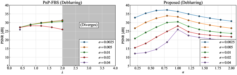
Figure 2: The influence of parameter variation on the restoration performance for PnP-FBS [17] and the proposed method. The plotted values are the average of seven images from ImageNet [63]. In PnP-FBS, we cannot obtain PSNR values when $\lambda>2$.

We performed two types of experiments to demonstrate the stability, performance, and versatility of the proposed method. The first experiment involves deblurring/inpainting under Gaussian noise, and the second experiment involves deblurring/inpainting under Poisson noise. The purpose of these experiments is to confirm the following two facts:

• The proposed method operates stably and converges in all experimental settings.

• In comparison to other state-of-the-art methods, the proposed method demonstrates higher restoration performance thanks to its stability.

IV-A Experimental Setup

In the two experiments, we considered two types of observation operators, one for blur and the other for random sampling. For the blur case, the operator $\mathbf{\Phi}$ was considered as a circular convolution with a $19\times 19$ kernel size [64, kernel 1]. This kernel was normalized so that $\|\mathbf{\Phi}\|_{\mathrm{op}}$ was equal to $1$. In the case of random sampling, pixels of the image were randomly selected and masked. The random sampling rate was set to $80\%$ for all cases.

We evaluated the restoration performance by Peak Signal to Noise Ratio (PSNR) and Structural Similarity Index Measure (SSIM). To investigate stability, the update rate $c_{n}$ for $n\in\mathbb{N}\backslash\{0\}$ was defined by $c_{n}:={\|\mathbf{u}_{n}-\mathbf{u}_{n-1}\|_{2}}/{\|\mathbf{u}_{n-1}\|_{2}},$ where $\mathbf{u}_{n}$ is the image at the $n$-th iteration by each algorithm.

We used color images for Gaussian noise case and grayscale images for Poisson noise case. The color images were randomly sampled from ImageNet[63], consisting of $7$ images cropped to $128\times 128$ pixels. The grayscale images were selected from 3 widely used image sets [17], all with a size of $256\times 256$ pixels.

In each experiment, we selected the appropriate methods from PnP-FBS [17], PnP-ADMM [24], PnP-PDS (Unstable) [25], PnP-PDS (w/o a box const.) [26], TV [59], and RED [44], and compared them with the proposed method. PnP-PDS (Unstable) was constructed with the same algorithm as the proposed method but employed DnCNN [32], which was not necessarily firmly nonexpansive. For TV, we used PDS to solve the optimization problems, which consisted of a total variation (TV) regularization term and the same data-fidelity term as the proposed method. For RED, we employed the steepest descent method for the case of Gaussian noise and PDS for the case of Poisson noise. Details of PnP-FBS, PnP-ADMM, and RED are given in Section III-C. In all methods, the number of iterations was fixed at 1200 for the blur case and 3000 for the random sampling case.

For fair comparison, the same DnCNN distributed by Pesquet et al.[17] was used for regularization in PnP-FBS, PnP-ADMM, PnP-PDS (w/o a box const.), RED, and the proposed method. This denoiser was a firmly nonexpansive DnCNN trained on Gaussian noise with a standard deviation of $0.01$. See [17] for details of the training. All of our experiments were conducted on Windows 11, equipped with an Intel Core i9 3.70GHz processor and 32.0GB of RAM.

IV-B Deblurring/inpainting under Gaussian noise

	Deblurring					Inpainting
Noise level $\sigma$	$0.0025$	$0.005$	$0.01$	$0.02$	$0.04$	$0.0025$	$0.005$	$0.01$	$0.02$	$0.04$
PnP-FBS [17]	$31.28$	$31.16$	$30.59$	$\underline{28.26}$	$25.94$	$--$	$--$	$--$	$--$	$--$
PnP-PDS (Unstable) [25]	$23.79$	$23.67$	$23.78$	$24.60$	$23.35$	$33.65$	$33.36$	$32.79$	$31.51$	$29.58$
PnP-PDS (w/o a box const.) [26]	$\underline{37.23}$	$\underline{34.03}$	$\underline{31.00}$	$28.24$	$\mathbf{26.00}$	$--$	$--$	$--$	$--$	$--$
TV [59]	$31.97$	$30.40$	$28.78$	$27.10$	$25.38$	$\underline{34.19}$	$\underline{33.90}$	$\underline{33.22}$	$\underline{31.90}$	$\underline{29.85}$
RED [44]	$34.11$	$33.38$	$30.89$	$\mathbf{28.30}$	$24.87$	$--$	$--$	$--$	$--$	$--$
PnP-PDS (Proposed)	$\mathbf{37.24}$	$\mathbf{34.04}$	$\mathbf{31.01}$	$\underline{28.26}$	$\mathbf{26.00}$	$\mathbf{35.61}$	$\mathbf{35.25}$	$\mathbf{34.43}$	$\mathbf{33.04}$	$\mathbf{31.00}$

TABLE II: The average PSNR [dB] values for deblurring and inpainting on the seven images from ImageNet[63]. The best value is highlighted in bold, and the second-best value is underlined.

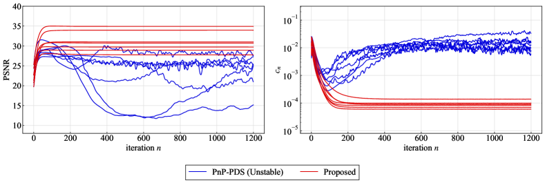
Figure 3: The evolution of PSNR and $c_{n}$ of PnP-PDS (Unstable) and the proposed method over iterations for deblurring at $\sigma=0.01$. Each plot in the graph corresponds to each image extracted from ImageNet.

(a) (PSNR, SSIM)
Ground truth

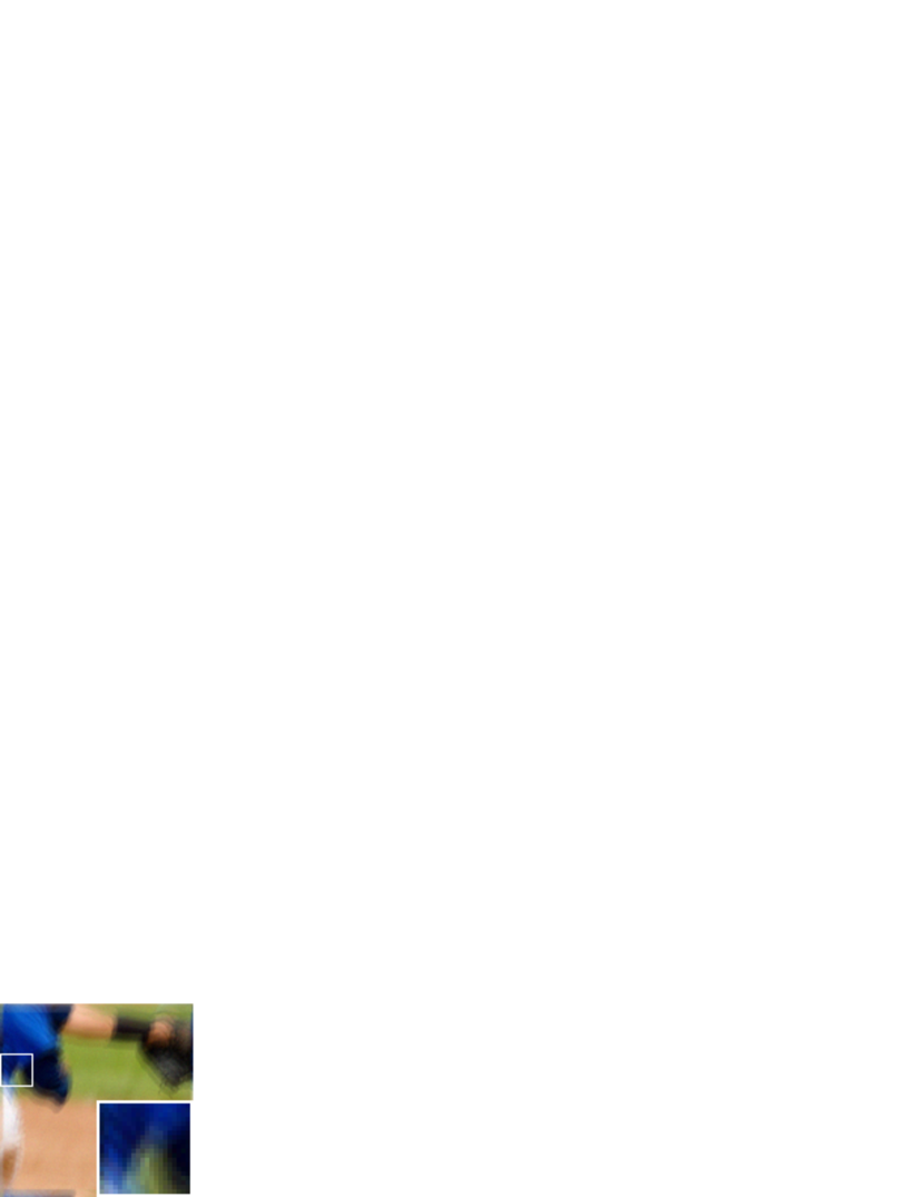
(b) $(21.29,\,0.6381)$
Observation

(c) $(33.47,\,0.9273)$
PnP-FBS

(d) $(27.55,\,0.8465)$
PnP-PDS
(Unstable)

(e) $(\underline{33.93},\,\underline{0.9313})$
PnP-PDS
(w/o a box const.)

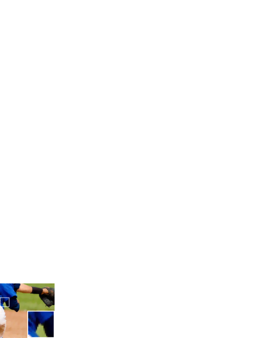
(f) $(30.53,\,0.8875)$
TV

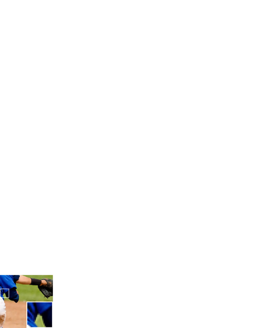
(g) $(33.75,\,0.9261)$
RED

(h) $(\mathbf{33.97},\,\mathbf{0.9317})$
Proposed

Figure 4: Visual results of image restoration on ImageNet for deblurring at $\sigma=0.01$. The number of iterations for all algorithms was fixed at $1200$. The best results are indicated in bold, and the second-best results are underlined.

IV-B1 Comparison of Parameter Robustness

First, we compare the robustness against parameter settings between PnP-FBS and the proposed method. As mentioned in Section III-C1, the proposed method handles constrained image restoration, which provides higher robustness in terms of parameter tuning. More specifically, it is reasonable to set $\varepsilon$ in (40) using the standard deviation $\sigma$ of the Gaussian noise as $\varepsilon=\alpha\sigma\sqrt{N}$, where $\alpha\in\mathbb{R}$ is a hyperparameter expected to be close to $1$ (note that the expected value of the $\ell_{2}$-norm of the Gaussian noise with the standard deviation $\sigma$ overlaid on the image $\mathbf{x}\in\mathbb{R}^{N}$ is given by $\sigma\sqrt{N}$). For the proposed method, the stepsizes $\gamma_{1}$ and $\gamma_{2}$ were set to $0.5$ and $0.99$ respectively, satisfying the conditions presented in Proposition 3.2.

Fig. 2 shows the variation in restoration performance across different $\alpha$ and $\lambda$ values. In PnP-FBS, the optimal value of $\lambda$ differs depending on the noise level, making it challenging to obtain the appropriate parameter value. Moreover, Fig. 2 also illustrates that the PSNR values cannot be obtained for PnP-FBS in the range of $\lambda>2$, as the pixel values of the estimated images diverge. The small $\sigma$ (i.e., the low noise level) requires prioritizing the data-fidelity term over regularization, resulting in a larger $\lambda$ value. However, a convergence issue arises for $\lambda>2$ because the condition in (47) is not satisfied. In fact, the plots for deblurring at $\sigma=0.005$ and $0.0025$ in Fig. 2 are expected to peak at $\lambda$ greater than $2$, where the algorithm shows unstable behavior and diverges. Additionally, for $\sigma=0.04$ (i.e., the high noise level), the denoiser may not maintain its firmly nonexpansiveness, leading to the divergence of PnP-FBS.

Conversely, the optimal value of $\alpha$ in the proposed method is approximately $1$ across all cases. This robustness suggests that the choice of $\alpha$ is independent of the noise level, simplifying the parameter setting (see also the discussion in Section III-C1). Moreover, the proposed method produces a valid image for any value of $\alpha$, indicating its consistent behavior. This stability can be attributed to the fact that the value of $\alpha$ does not influence the convergence of the algorithm.

Remark 3.

Regarding the parameter settings for PnP-FBS, heuristics for determining $\lambda$ are proposed in [17]. However, the theoretical justification of this approach is still an open problem (see [17, Section 4.2] for details).

IV-B2 Comparison of Restoration Performance

	Deblurring			Inpainting
Scaling coefficient $\eta$	$50$	$100$	$200$	$50$	$100$	$200$
PnP-ADMM [24]	$25.16$	$26.28$	$26.55$	$11.45$	$27.87$	$28.10$
PnP-PDS (Unstable) [25]	$23.98$	$25.18$	$26.51$	$\mathbf{29.75}$	$\mathbf{31.90}$	$\mathbf{33.43}$
PnP-PDS (w/o a box const.) [26]	$\mathbf{25.17}$	$\underline{26.42}$	$\mathbf{27.77}$	$\mathbf{29.75}$	$\underline{31.21}$	$\underline{32.74}$
RED [44]	$25.13$	$26.39$	$27.72$	$29.71$	$31.19$	$32.69$
PnP-PDS (Proposed)	$\mathbf{25.17}$	$\mathbf{26.44}$	$\mathbf{27.77}$	$\mathbf{29.75}$	$\underline{31.21}$	$\underline{32.74}$

TABLE III: The average PSNR [dB] values for deblurring and inpainting on the three images from Set3[17]. The best value is highlighted in bold, and the second-best value is underlined.

	Deblurring			Inpainting
Scaling coefficient $\eta$	$50$	$100$	$200$	$50$	$100$	$200$
PnP-ADMM [24]	$1.692$	$2.224$	$2.898$	$1.203$	$0.6317$	$0.9953$
PnP-PDS (Proposed)	$0.6523$	$0.6465$	$0.6529$	$0.4005$	$0.4030$	$0.4039$

TABLE IV: The average CPU time [s] per iteration for deblurring and inpainting on the three images from Set3[17].

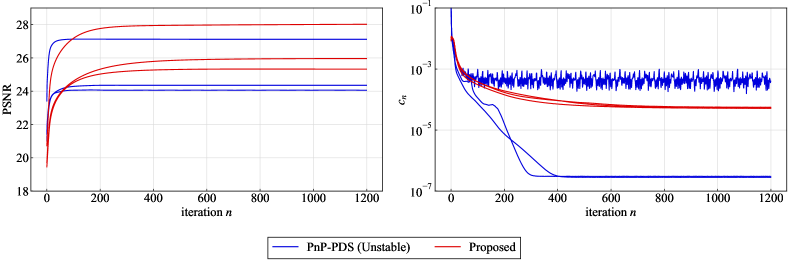
Figure 5: The evolution of PSNR and $c_{n}$ of PnP-PDS (Unstable) and the proposed method over iterations for deblurring at $\eta=100$. Each plot in the graph corresponds to each image extracted from Set3[17]

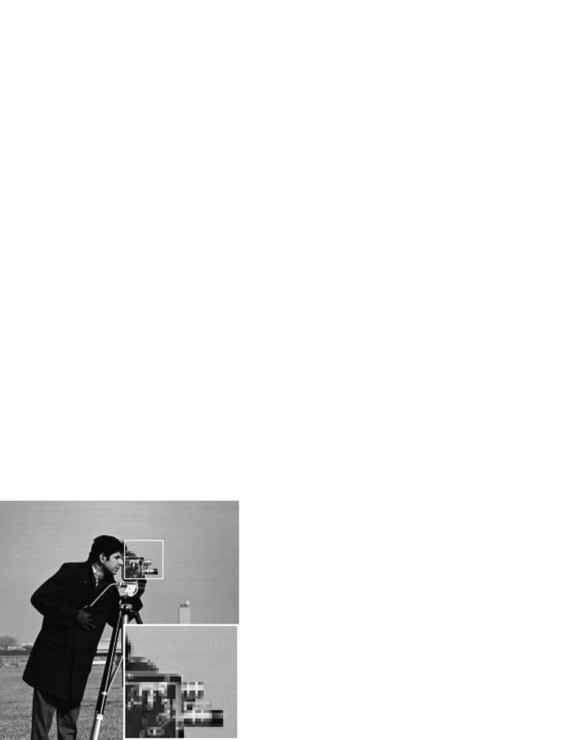
(a) (PSNR, SSIM)
Ground truth

(b) $(19.26,\,0.2653)$
Observation

(c) $(25.17,\,\mathbf{0.7743})$
PnP-ADMM

(d) $(24.05,\,0.7618)$
PnP-PDS
(Unstable)

(e) $(\underline{25.31},\,0.7731)$
PnP-PDS
(w/o a box const.)

(f) $(\underline{25.31},\,0.7678)$
RED

(g) $(\mathbf{25.33},\,\underline{0.7733})$
Proposed

Figure 6: Visual results of image restoration on Set3 for deblurring at $\eta=100$. The number of iterations for all algorithms was fixed at $1200$. The best results are indicated in bold, and the second-best results are underlined.

We compare the performance of the proposed method with other methods, namely PnP-FBS[17], PnP-PDS (Unstable)[25], PnP-PDS (w/o a box const.) [26], TV[59], and RED[44]. For constrained formulations such as PnP-PDS (Unstable), PnP-PDS (w/o a box const.), TV, and the proposed method, we set $\varepsilon=\alpha\sigma\sqrt{N}$ in the same way as in the previous section. For each of these methods, we performed a linear search for $\alpha$ to evaluate the restoration performance. Specifically, we found the best $\alpha$ values in the proposed method were $[0.82,\,0.86,\,0.92,\,0.96,\,1.0]$ for deblurring and $[0.90,\,0.82,\,0.82,\,1.0,\,1.0]$ for inpainting, corresponding to $\sigma=[0.0025,\,0.005,\,0.01,\,0.02,\,0.04]$, respectively. The balancing parameters for the other methods were also determined through a linear search. The stepsizes $\gamma_{1}$ and $\gamma_{2}$ in the proposed method were set to $0.5$ and $0.99$, respectively, satisfying the condition in Proposition 3.2.

Table II shows the average PSNR values over seven images, obtained with the optimal parameters for each method. Most importantly, the proposed method demonstrates superior performance compared to PnP-FBS, even though both methods employ the same denoiser for regularization. This is attributed to the difference in the ease of finding suitable parameters. As mentioned in Section IV-B1, the appropriate value of the parameter $\varepsilon$ in the proposed method, can be easily found using the standard deviation of the Gaussian noise. On the other hand, the parameter $\lambda$ in PnP-FBS, lacks a clear interpretation, making it difficult to set appropriate values. The experimental results also confirm that the proposed method outperforms PnP-PDS (Unstable), PnP-PDS (w/o a box const.), TV, and RED.

Furthermore, in the case of inpainting by PnP-FBS, PnP-PDS (w/o a box const.), and RED, the algorithms do not converge and PSNR values are not obtained. One possible explanation for this is that the condition in (16) does not hold for images with extreme pixel values, such as masking pixels. Meanwhile, the proposed method achieves stable behavior and satisfactory performance even in the random sampling setting. This is due to the box constraint, which ensures that the pixel values of the images remain within the range of $[0,\,1]$.

To compare the convergence and stability of the proposed method, we show the evolution of PSNR and the update rate $c_{n}$ at each iteration for deblurring at $\sigma=0.01$ in Fig. 3. For the proposed method, the value of $c_{n}$ decreases to approximately $10^{-5}$ and shows a convergent evolution. In contrast, PnP-PDS (Unstable), which uses a denoiser that is not necessarily firmly nonexpansive, shows inconsistent behavior.

In Fig. 4, we provide the visual results of deblurring at $\sigma=0.01$, accompanied by PSNR (left) and SSIM (right). The images obtained by PnP-FBS and TV are overly-smoothed, resulting in a loss of fine detail. In the case of PnP-PDS (Unstable), strong artifacts are generated due to the unstable behavior of the algorithm (see the top-right corner of the image). While RED achieves high PSNR and SSIM, there are some areas where the brightness appears unnaturally altered compared to the original image. The proposed method achieves the highest PSNR and SSIM for this image of all the methods compared, presenting the most natural appearance.

IV-C Deblurring/inpainting under Poisson noise

Let us now present the experiments on deblurring/inpainting under Poisson noise. We considered three different scaling coefficients $\eta$ for the Poisson noise level, i.e. $50$, $100$, and $200$. Smaller values of $\eta$ correspond to stronger noise, while larger values indicate weaker noise. We compare the performance of the proposed method with other state-of-the-art methods applicable to this scenario, specifically PnP-ADMM [24], PnP-PDS (Unstable) [25], PnP-PDS (w/o a box const.) [26], and RED [44]. For all methods, we performed a linear search for the balancing parameters. The best $\lambda$ values in the proposed method were $[0.00125,\,0.00125,\,0.001]$ for deblurring and $[0.00075,\,0.0005,\,0.0005]$ for inpainting, corresponding to $\eta=[50,\,100,\,200]$, respectively. The stepsizes $\gamma_{1}$ and $\gamma_{2}$ were set to $0.5$ and $0.99$, respectively, the same as in the case of deblurring/inpainting under Gaussian noise.

The average PSNR values over three images are presented in Table III. The proposed method shows high restoration performance across all settings. Although PnP-PDS (w/o a box const.) achieves comparable results, the proposed method demonstrates slightly better performance in certain cases, thanks to its enhanced stability. Moreover, the proposed method outperforms the other state-of-the-art methods with higher PSNR values.

We investigate the computational efficiency of the proposed method, particularly in comparison with PnP-ADMM. Table IV provides the CPU times per iteration for PnP-ADMM and the proposed method. As discussed in Section III-C2, we need to perform inner iterations for PnP-ADMM, leading to relatively high computational costs. The proposed method reduces CPU times by half compared to PnP-ADMM in all settings, since it solves the problem in (43) without inner iterations.

To evaluate the stability, we present PSNR and the update rate $c_{n}$ at each iteration in the proposed method and PnP-PDS (Unstable) in Fig. 5. For PnP-PDS (Unstable), $c_{n}$ exhibits inconsistently depending on the image. In contrast, the proposed method shows a consistent decrease in $c_{n}$ over iterations, along with stable PSNR values, indicating the stable behavior of the proposed method.

Finally, we present the visual results of the deblurring at $\eta=100$ with PSNR (left) and SSIM (right) in Fig 6. PnP-PDS (Unstable) loses the details of the original images, while PnP-ADMM, RED, and PnP-PDS (w/o a box const.) show slight changes in brightness or fine shapes. In contrast, the proposed method preserves fine details, resulting in an image that appears visually natural.

V Conclusion

In this paper, we have proposed a general PnP-PDS method with a theoretical convergence guarantee under realistic assumptions in real-world settings, supported by extensive experimental results. First, we provided a theoretical proof that the proposed PnP-PDS converges when the denoiser is firmly nonexpansive, which is a realistic assumption for practical applications. Then, we showed that it efficiently solves various image restoration problems involving nonsmooth data-fidelity terms and additional hard constraints without the need to compute matrix inversions or perform inner iterations. Finally, through numerical experiments on deblurring/inpainting under Gaussian noise and deblurring/inpainting under Poisson noise, we demonstrated that the proposed PnP-PDS outperforms existing methods with stable convergence behavior. We believe that the proposed PnP-PDS holds great potential for a wide range of applications including biomedical imaging, astronomical imaging, and remote sensing.

References

- [1] L. I. Rudin, S. Osher, and E. Fatemi, “Nonlinear total variation based noise removal algorithms,” Physica D, vol. 60, pp. 259–268, 1992.
- [2] K. Bredies, K. Kunisch, and T. Pock, “Total generalized variation,” SIAM J. Imag. Sci., vol. 3, no. 3, p. 492–526, 2010.
- [3] S. Ono and I. Yamada, “Decorrelated vectorial total variation,” in Proc. IEEE Conf. Comput. Vis. Pattern Recognit. (CVPR), 2014, pp. 4090–4097.
- [4] S. Lefkimmiatis, A. Roussos, P. Maragos, and M. Unser, “Structure tensor total variation,” SIAM J. Imag. Sci., vol. 8, no. 2, pp. 1090–1122, 2015.
- [5] L. Condat, “Discrete total variation: New definition and minimization,” SIAM J. Imag. Sci., vol. 10, no. 3, pp. 1258–1290, 2017.
- [6] P. L. Combettes and J. C. Pesquet, Proximal Splitting Methods in Signal Processing. Springer New York, 2011, pp. 185–212.
- [7] N. Parikh and S. Boyd, “Proximal algorithms,” Found. Trends Optim., vol. 1, no. 3, pp. 127–239, 2014.
- [8] L. Condat, D. Kitahara, A. Contreras, and A. Hirabayashi, “Proximal splitting algorithms for convex optimization: A tour of recent advances, with new twists,” SIAM Rev., vol. 65, no. 2, pp. 375–435, 2023.
- [9] P. L. Combettes and V. R. Wajs, “Signal recovery by proximal forward-backward splitting,” Multiscale Modeling & Simulation, vol. 4, no. 4, pp. 1168–1200, 2005.
- [10] S. Boyd, N. Parikh, E. Chu, B. Peleato, and J. Eckstein, “Distributed optimization and statistical learning via the alternating direction method of multipliers,” Found. Trends Mach. Learn., vol. 3, pp. 1–122, 2011.
- [11] A. Chambolle and T. Pock, “A first-order primal-dual algorithm for convex problems with applications to imaging,” J. Math. Imag. Vis., vol. 40, no. 1, pp. 120–145, 2010.
- [12] P. L. Combettes and J. C. Pesquet, “Primal-dual splitting algorithm for solving inclusions with mixtures of composite, lipschitzian, and parallel-sum type monotone operators,” Set-Valued Var. Anal., vol. 20, no. 2, p. 307–330, 2012.
- [13] L. Condat, “A primal-dual splitting method for convex optimization involving lipschitzian, proximable and linear composite terms,” J Opt. Theory Appl., vol. 158, no. 2, pp. 460–479, 2013.
- [14] B. C. Vu, “A splitting algorithm for dual monotone inclusions involving cocoercive operators,” Adv. Comput. Math., vol. 38, no. 3, p. 667–681, 2013.
- [15] P. L. Combettes, L. Condat, J. C. Pesquet, and B. Vu, “A forward-backward view of some primal-dual optimization methods in image recovery,” in Proc. IEEE Int. Conf. Image Process. (ICIP), 2014, pp. 4141–4145.
- [16] L. Condat, “A generic proximal algorithm for convex optimization—application to total variation minimization,” IEEE Signal Process. Lett., vol. 21, no. 8, pp. 985–989, 2014.
- [17] J. C. Pesquet, A. Repetti, M. Terris, and Y. Wiaux, “Learning maximally monotone operators for image recovery,” SIAM J. Imag. Sci., vol. 14, no. 3, pp. 1206–1237, 2021.
- [18] A. Ebner and M. Haltmeier, “Plug-and-play image reconstruction is a convergent regularization method,” IEEE Trans. Image Process., vol. 33, p. 1476–1486, 2024.
- [19] S. V. Venkatakrishnan, C. A. Bouman, and B. Wohlberg, “Plug-and-play priors for model based reconstruction,” in Proc. IEEE Global Conf. Signal and Inf. Process., 2013, pp. 945–948.
- [20] A. Rond, R. Giryes, and M. Elad, “Poisson inverse problems by the plug-and-play scheme,” J. Vis. Comm. and Imag. Rep., vol. 41, pp. 96–108, 2016.
- [21] S. Sreehari, S. V. Venkatakrishnan, B. Wohlberg, G. T. Buzzard, L. F. Drummy, J. P. Simmons, and C. A. Bouman, “Plug-and-play priors for bright field electron tomography and sparse interpolation,” IEEE Trans. Comput. Imag., vol. 2, no. 4, p. 408–423, 2016.
- [22] S. H. Chan, X. Wang, and O. A. Elgendy, “Plug-and-play ADMM for image restoration: Fixed-point convergence and applications,” IEEE Trans. Comput. Imag., vol. 3, no. 1, pp. 84–98, 2017.
- [23] P. Nair, R. G. Gavaskar, and K. N. Chaudhury, “Fixed-point and objective convergence of plug-and-play algorithms,” IEEE Trans. Comput. Imag., vol. 7, pp. 337–348, 2021.
- [24] Y. Sun, Z. Wu, X. Xu, B. Wohlberg, and U. S. Kamilov, “Scalable plug-and-play ADMM with convergence guarantees,” IEEE Trans. Comput. Imag., vol. 7, pp. 849–863, 2021.
- [25] S. Ono, “Primal-dual plug-and-play image restoration,” IEEE Signal Process. Lett., vol. 24, no. 8, pp. 1108–1112, 2017.
- [26] C. S. Garcia, M. Larchevêque, S. O’Sullivan, M. V. Waerebeke, R. Thomson, A. Repetti, and J.-C. Pesquet, “A primal–dual data-driven method for computational optical imaging with a photonic lantern,” PNAS Nexus, vol. 3, no. 4, p. 164, 2024.
- [27] A. Danielyan, V. Katkovnik, and K. Egiazarian, “BM3D frames and variational image deblurring,” IEEE Trans. Image Process., vol. 21, no. 4, pp. 1715–1728, 2012.
- [28] J. Zhang, D. Zhao, and W. Gao, “Group-based sparse representation for image restoration,” IEEE Trans. Image Process., vol. 23, no. 8, pp. 3336–3351, 2014.
- [29] K. Dabov, A. Foi, V. Katkovnik, and K. Egiazarian, “Image denoising by sparse 3-D transform-domain collaborative filtering,” IEEE Trans. Image Process., vol. 16, no. 8, pp. 2080–2095, 2007.
- [30] A. Buades, B. Coll, and J.-M. Morel, “Non-local means denoising,” Imag. Process. On Line, vol. 1, pp. 208–212, 2011.
- [31] Y. Chen and T. Pock, “Trainable nonlinear reaction diffusion: A flexible framework for fast and effective image restoration,” IEEE Trans. Pattern Anal. Mach. Intell., vol. 39, no. 6, pp. 1256–1272, 2017.
- [32] K. Zhang, W. Zuo, Y. Chen, D. Meng, and L. Zhang, “Beyond a gaussian denoiser: Residual learning of deep cnn for image denoising,” IEEE Trans. Image Process., vol. 26, no. 7, p. 3142–3155, 2017.
- [33] Z. Wu, Y. Sun, A. Matlock, J. Liu, L. Tian, and U. Kamilov, “SIMBA: Scalable inversion in optical tomography using deep denoising priors,” IEEE J. of Sel. Top. Signal Process., vol. 14, no. 6, pp. 1163–1175, 2020.
- [34] R. Ahmad, C. A. Bouman, G. T. Buzzard, S. Chan, S. Liu, E. T. Reehorst, and P. Schniter, “Plug-and-play methods for magnetic resonance imaging: Using denoisers for image recovery,” IEEE Signal Process. Mag., vol. 37, no. 1, pp. 105–116, 2020.
- [35] C. Pellizzari, M. Spencer, and C. Bouman, “Coherent plug-and-play: Digital holographic imaging through atmospheric turbulence using model-based iterative reconstruction and convolutional neural networks,” IEEE Trans. Comput. Imag., vol. 6, pp. 1–1, 12 2020.
- [36] G. T. B. U. S. Kamilov, C. A. Bouman and B. Wohlberg, “Plug-and-play methods for integrating physical and learned models in computational imaging,” IEEE Signal Process. Mag., vol. 40, no. 1, pp. 85–97, 2023.
- [37] K. Zhang, Y. Li, W. Zuo, L. Zhang, L. Van Gool, and R. Timofte, “Plug-and-play image restoration with deep denoiser prior,” IEEE Trans. Pattern Anal. Mach. Intell., vol. 44, no. 10, p. 6360–6376, 2022.
- [38] M. Duff, N. D. F. Campbell, and M. J. Ehrhardt, “Regularising inverse problems with generative machine learning models,” J. Math. Imag. Vis., vol. 66, pp. 37–56, 2024.
- [39] D. P. Kingma and M. Welling, “An introduction to variational autoencoders,” Found. Trends Mach. Learn., vol. 12, no. 4, p. 307–392, 2019.
- [40] M. Arjovsky, S. Chintala, and L. Bottou, “Wasserstein generative adversarial networks,” in Proc. Int. Conf. Mach. Learn. (ICML), ser. Proc. Mach. Learn. Research, 2017, pp. 214–223.
- [41] P. Dhariwal and A. Nichol, “Diffusion models beat gans on image synthesis,” in Proc. Conf. Neural Inf. Process. Sys. (NeurIPS), 2021, p. 8780–8794.
- [42] Y. Zhu, K. Zhang, J. Liang, J. Cao, B. Wen, R. Timofte, and L. V. Gool, “Denoising diffusion models for plug-and-play image restoration,” in IEEE Conf. Comput. Vis. Pattern Recognit. Workshops (CVPRW), 2023, pp. 1219–1229.
- [43] E. Ryu, J. Liu, S. Wang, X. Chen, Z. Wang, and W. Yin, “Plug-and-play methods provably converge with properly trained denoisers,” in Proc. Int. Conf. Mach. Learn. (ICML), 2019, pp. 5546–5557.
- [44] Y. Romano, M. Elad, and P. Milanfar, “The little engine that could: regularization by denoising (RED),” SIAM J. Imag. Sci., vol. 10, no. 4, p. 1804–1844, 2017.
- [45] R. Cohen, M. Elad, and P. Milanfar, “Regularization by denoising via fixed-point projection (RED-PRO),” SIAM J. Imag. Sci., vol. 14, no. 3, pp. 1374–1406, 2021.
- [46] R. Cohen, Y. Blau, D. Freedman, and E. Rivlin, “It has potential: Gradient-driven denoisers for convergent solutions to inverse problems,” in Proc. Conf. Neural Inf. Process. Sys. (NeurIPS), 2021, pp. 18 152–18 164.
- [47] S. Hurault, A. Leclaire, and N. Papadakis, “Gradient step denoiser for convergent plug-and-play,” in Int. Conf. Learn. Represent., 2022.
- [48] S. Hurault, A. Leclaire, and N. Papadakis, “Proximal denoiser for convergent plug-and-play optimization with nonconvex regularization,” in Proc. Int. Conf. Mach. Learn. (ICML), 2022, pp. 9483–9505.
- [49] H. Y. Tan, S. Mukherjee, J. Tang, and C.-B. Schönlieb, “Provably convergent plug-and-play quasi-newton methods,” SIAM J. Imag. Sci., vol. 17, no. 2, pp. 785–819, 2024.
- [50] E. T. Reehorst and P. Schniter, “Regularization by denoising: Clarifications and new interpretations,” IEEE Trans. Comput. Imag., vol. 5, no. 1, pp. 52–67, 2019.
- [51] Y. Suzuki, R. Isono, and S. Ono, “A convergent primal-dual deep plug-and-play algorithm for constrained image restoration,” in Proc. IEEE Int. Conf. Acoust., Speech Signal Process. (ICASSP), 2024, pp. 9541–9545.
- [52] H. H. Bauschke and P. L. Combettes, Correction to: Convex Analysis and Monotone Operator Theory in Hilbert Spaces, 2nd ed. Springer Int. Publishing, 2017.
- [53] J. J. Moreau, “Fonctions convexes duales et points proximaux dans un espace hilbertien,” Comptes Rendus de l ’Academie Bulg. des Sci., vol. 255, p. 2897–2899, 1962.
- [54] P. Combettes and N. N. Reyes, “Moreau’s decomposition in banach spaces,” Math. Program., vol. 139, no. 1-2, pp. 103–114, 2013.
- [55] G. H. Golub and C. F. V. Loan, Matrix computations. JHU press, 2013.
- [56] R. Bhatia and F. Kittaneh, “Norm inequalities for partitioned operators and an application,” Math. Ann., vol. 287, pp. 719–726, 1990.
- [57] G. Chierchia, N. Pustelnik, J. Pesquet, and B.Pesquet, “Epigraphical projection and proximal tools for solving constrained convex optimization problems,” Signal, Image and Video Process., vol. 9, no. 8, pp. 1737–1749, 2015.
- [58] S. Ono, “Efficient constrained signal reconstruction by randomized epigraphical projection,” in Proc. IEEE Int. Conf. Acoust., Speech Signal Process. (ICASSP), 2019, pp. 4993–4997.
- [59] M. Afonso, J. Bioucas-Dias, and M. Figueiredo, “An augmented lagrangian approach to the constrained optimization formulation of imaging inverse problems,” IEEE Trans. Image Process., vol. 20, no. 3, pp. 681–95, 2011.
- [60] S. Ono and I. Yamada, “Signal recovery with certain involved convex data-fidelity constraints,” IEEE Trans. Signal Process., vol. 63, no. 22, pp. 6149–6163, 2015.
- [61] S. Ono, “ gradient projection,” IEEE Trans. Image Process., vol. 26, no. 4, pp. 1554–1564, 2017.
- [62] P. L. Combettes and J.-C. Pesquet, “A douglas–rachford splitting approach to nonsmooth convex variational signal recovery,” IEEE J. of Sel. Topics in Signal Process., vol. 1, no. 4, pp. 564–574, 2007.
- [63] J. Deng, W. Dong, R. Socher, L. J. Li, K. Li, and L. Fei-Fei, “Imagenet: A large-scale hierarchical image database,” in Proc. IEEE Conf. Comput. Vis. Pattern Recognit. (CVPR), 2009, pp. 248–255.
- [64] A. Levin, Y. Weiss, F. Durand, and W. T. Freeman, “Understanding and evaluating blind deconvolution algorithms,” in Proc. IEEE Conf. Comput. Vis. Pattern Recognit. (CVPR), 2009, pp. 1964–1971.