Group Sparse-based Tensor CP Decomposition: Model, Algorithms, and Applications in Chemometrics

Abstract

The CANDECOMP/PARAFAC (or Canonical polyadic, CP) decomposition of tensors has numerous applications in various fields, such as chemometrics, signal processing, machine learning, etc. Tensor CP decomposition assumes the knowledge of the exact CP rank, i.e., the total number of rank-one components of a tensor. However, accurately estimating the CP rank is very challenging. In this work, to address this issue, we prove that the CP rank can be exactly estimated by minimizing the group sparsity of any one of the factor matrices under the unit length constraints on the columns of the other factor matrices. Based on this result, we propose a CP decomposition model with group sparse regularization, which integrates the rank estimation and the tensor decomposition as an optimization problem, whose set of optimal solutions is proved to be nonempty. To solve the proposed model, we propose a double-loop block-coordinate proximal gradient descent algorithm with extrapolation and prove that each accumulation point of the sequence generated by the algorithm is a stationary point of the proposed model. Furthermore, we incorporate a rank reduction strategy into the algorithm to reduce the computational complexity. Finally, we apply the proposed model and algorithms to the component separation problem in chemometrics using real data. Numerical experiments demonstrate the robustness and effectiveness of the proposed methods.

Key words: CP decomposition, group sparse, double-loop, block-coordinate proximal gradient descent, extrapolation, rank reduction

1 Introduction

Tensor decomposition can reveal underlying information in data analysis and is widely used in various fields [13]. The CANDECOMP/PARAFAC (CP) decomposition [4, 10], also known as the canonical polyadic decomposition [11], is one of the most important tasks in the decomposition of tensors. The CP decomposition of a given tensor $\mathcal{X}\in\mathds{R}^{n_{1}\times\cdots\times n_{N}}$ factorizes $\mathcal{X}$ into a sum of rank-one component tensors and takes the following form:

$$\mathcal{X}=[\![{\mathbf{A}}^{(1)},\cdots,{\mathbf{A}}^{(N)}]\!]:=\sum_{r=1}^{R}\mathbf{a}^{(1)}_{r}\circ\cdots\circ{\mathbf{a}}^{(N)}_{r},$$ (1)

where $R$ is a positive integer, $\mathbf{a}^{(i)}_{r}\in\mathds{R}^{n_{i}},r=1,\cdots,R$, represents the $r$-th column of the factor matrix $\mathbf{A}^{(i)}\in\mathds{R}^{n_{i}\times R},i=1,\cdots,N$, and the symbol $\circ$ represents the outer product. In this expression, the CP rank of $\mathcal{X}$, denoted $\rm rank_{cp}(\mathcal{X})$, is defined as the smallest number of rank-one tensors, that is, the smallest $R$ such that (1) holds [13]. If $R=\rm rank_{cp}(\mathcal{X})$ in (1), then it is called the $\rm rank$ CP decomposition [13]. The uniqueness of the decomposition of CP under mild assumptions [9, 14, 22] leads to countless applications in chemometrics [17, 32, 33], signal processing [19, 21], machine learning [18, 23], neuroscience [7, 8], and hyperspectral imaging [25, 34], to name only a few. One may refer to surveys such as [1, 5, 6, 13] for a more general background.

Numerous CP decomposition models and the corresponding algorithms have been developed, with the assumption of a fixed CP rank, i.e., the number of rank-one components. The most widely studied CP decomposition model is the unconstrained optimization problem by minimizing the least squares (LS) loss function. Several algorithms have been proposed to solve this unconstrained optimization model. Harshman [10] first introduced the parallel factor analysis (PARAFAC) algorithm. Wu et al. [31] proposed an alternating trilinear decomposition algorithm (ATLD) for the trilinear decomposition model in chemometrics, i.e., the CP decomposition model. Kolda et al. [2, 16] developed randomized CP decomposition algorithms for large-scale dense and sparse tensors. Wang et al. [27, 28] proposed accelerated stochastic gradient descent algorithms for large-scale tensor CP decomposition. In recent years, CP decomposition models with constraints, such as orthogonal, nonnegative and column unit constraints, have been proposed for practical applications. For example, Yang [35] introduced an $\epsilon$ alternating least squares algorithm to solve the CP decomposition model with orthogonal constraints. Wang and Cong [26] studied the CP decomposition model with nonnegative constraints and introduced an inexact accelerated proximal gradient (iAPG) algorithm to solve it. Wang and Bai [30] introduced a CP decomposition model with nonnegative and column unit constraints for the component separation problem in complex chemical systems, and proposed an accelerated inexact block coordinate descent algorithm to solve the model.

Currently, one crucial challenge in CP decomposition models and algorithms is the requirement for accurately estimating the CP rank in advance. Deviations from the true CP rank may increase fitting errors and cause factor degeneracy. However, the tensor CP rank is NP-hard to compute [13] and there is no finite algorithm for determining the rank of a tensor [12, 15]. These observations naturally lead us to raise the following question: Can we establish a tensor CP decomposition model with CP rank estimation simultaneously?

To address this question, in this paper, we introduce a CP decomposition model with group sparse regularization given by

$$\begin{array}[]{lll}\min\limits_{\mathbf{A}^{(1)},\cdots,\mathbf{A}^{(N)}}&\frac{1}{2}\|\mathcal{X}-[\![\mathbf{A}^{(1)},\cdots,\mathbf{A}^{(N)}]\!]\|^{2}+\lambda\|\mathbf{A}^{(N)}\|_{2,0}\\ \text{ s.t. }&\|\mathbf{a}^{(i)}_{r}\|=1,i=1,\cdots,N-1,r=1\cdots R,\end{array}$$ (2)

where $\mathcal{X}\in\mathds{R}^{n_{1}\times\cdots\times n_{N}}$ is a given tensor and $\|\mathbf{A}^{(N)}\|_{2,0}:=\sum_{r=1}^{R}(\|\mathbf{a}^{(N)}_{r}\|)^{0}$. We establish the equivalence between the CP rank of a given tensor and minimizing the $\ell_{2,0}$ norm on one of the factor matrices under the unit length constraints on the columns of the others.

To solve the problem (2), we develop a double-loop block-coordinate proximal gradient descent algorithm with extrapolation. In this algorithm, each factor matrix is treated as a block and solved approximately by a block-coordinate proximal gradient descent algorithm with finitely many cycles. Additionally, extrapolation is applied after each factor matrix is updated, and a check to ensure the reduction of objective function value is performed after each outer iteration. We prove that each limit point of the sequence generated by the proposed algorithm is a stationary point of the model (2). Furthermore, we prove that for a convergent sequence $\{(\mathbf{A}^{(1)^{k}},\cdots,\mathbf{A}^{(N)^{k}})\}$, the nonzero columns of $\mathbf{A}^{(N)^{k}}$ remain unchanged after a certain number of iterations. Based on this result, we develop a rank reduction strategy to reduce computational complexity. The rank reduction strategy works as follows: if the nonzero columns of $\mathbf{A}^{(N)^{k}}$ remain unchanged, removing the zero columns in $\mathbf{A}^{(N)^{k}}$ and the corresponding columns in $\mathbf{A}^{(i)^{k}},i=1,\cdots,N-1$, and allowing the iterations to continue.

Eventually, we apply the proposed model and algorithms to the component separation problem in chemometrics. This problem involves resolving chemically meaningful independent component information from mixed-response signals, which can be formulated as a CP decomposition model. Accurate estimation of the number of components is crucial in this problem since incorrect estimation can lead to separation failure. Numerical experiments conducted on third-order real chemical data demonstrate that our proposed methods can precisely separate the components and accurately estimate their concentrations, even when the initial number of components is overestimated. This suggests that our proposed methods can simultaneously estimate the CP rank and obtain the CP decomposition of a given tensor.

The main contributions of this paper are threefold.

• We prove that determining the CP rank of a given tensor is equivalent to minimizing the $\ell_{2,0}$ norm on one of the factor matrices under the unit length constraints on the columns of the others. Based on this equivalence, we propose a CP decomposition model with group sparse regularization and unit length constraints, which can simultaneously estimate the CP rank and obtain the CP decomposition.

• We develop a double-loop block-coordinate proximal gradient descent algorithm with extrapolation to solve the proposed model and prove that each limit point of the sequence generated by this algorithm is a stationary point of the model. Furthermore, we demonstrate that for a convergent sequence $\{(\mathbf{A}^{(1)^{k}},\cdots,\mathbf{A}^{(N)^{k}})\}$, the nonzero columns of $\mathbf{A}^{(N)^{k}}$ remain unchanged after a certain number of iterations. Based on this observation, we develop a rank reduction strategy to reduce the computational complexity.

• We apply the proposed models and algorithms to solve the component separation problem in chemometrics. Numerical experiments on real data demonstrate the robustness and effectiveness of our proposed methods.

The remainder of this paper is organized as follows. First, in Section 2, some notations and definitions are introduced. Next, in Section 3, we prove the equivalent surrogate of the CP rank of a tensor and present a CP decomposition model with group sparse regularization and unit length constraints. After that, in Section 4, we develop a double-loop block-coordinate proximal gradient descent algorithm with extrapolation to solve our proposed model. We also provide a convergence analysis and incorporate a rank reduction strategy into the algorithm. Subsequently, in Section 5, we apply the proposed methods to the component separation problem in chemometrics. Eventually, the conclusions are drawn in Section 6.

2 Preliminaries

We introduce the definitions and notation used throughout this paper. Scalars, vectors, matrices, and tensors are denoted as lowercase letters ($x$), lowercase boldface letters ($\mathbf{x}$), boldface capital letters ($\mathbf{X}$), and calligraphic letters ($\mathcal{X}$), respectively. Sets are denoted as hollow letters, for example, $\mathbb{X}$. The real field is denoted by $\mathds{R}$. For a $N$-th order tensor $\mathcal{X}\in\mathds{R}^{n_{1}\times\cdots\times n_{N}}$, we denote its $(i_{1},\cdots,i_{N})$-th entry as ${X}_{i_{1},\cdots,i_{N}}$. The $i$-th column of the matrix $\mathbf{X}$ is denoted as $\mathbf{x}_{i}$. The transpose of the matrix $\mathbf{X}$ is denoted by $\mathbf{X}^{\top}$. The Frobenius norms for a tensor $\mathcal{X}$ and a matrix $\mathbf{X}$ are denoted by $\|\mathcal{X}\|$ and $\|\mathbf{X}\|$, respectively. The Euclidean norm for a vector $\mathbf{x}$ is denoted by $\|\mathbf{x}\|$. We use the symbols $\circ$, $\otimes$, and $\odot$ to represent the outer, Kronecker, and Khatri-Rao products, respectively. For a real vector $\mathbf{x}$, its zero norm $\|\mathbf{x}\|_{0}$ is the cardinality of its nonzero components. For a given matrix $\mathbf{X}=(\mathbf{X}_{1},\cdots,\mathbf{X}_{m})$, its $\ell_{2,0}$ norm is defined by $\|\mathbf{X}\|_{2,0}:=\|(\|\mathbf{X}_{1}\|,\cdots,\|\mathbf{X}_{m}\|)^{\top}\|_{0}$, and we denote

$$\mathbf{X}_{<i}:=(\mathbf{X}_{1},\cdots,\mathbf{X}_{i-1}),\quad\mathbf{X}_{\geq i}:=(\mathbf{X}_{i},\cdots,\mathbf{X}_{m}).$$

We use ${\rm supp}(\mathbf{X})$ to represent the index set of the nonzero columns of $\mathbf{X}$.

3 A regularized CP decomposition model

This section proposes a regularized CP decomposition model to obtain a rank CP decomposition of a given tensor. Recall that for a given tensor $\mathcal{X}\in\mathds{R}^{n_{1}\times\cdots\times n_{N}}$, as shown in (1), the CP decomposition factorizes $\mathcal{X}$ into a sum of rank-one tensors. The CP rank of $\mathcal{X}$, denoted by $\rm rank_{cp}(\mathcal{X})$, is defined as the smallest number of rank-one tensors that can constitute a CP decomposition, i.e., the smallest $R$ in (1). As mentioned in Section 1, most current CP decomposition models require an accurate prior estimation of the CP rank of $\mathcal{X}$ to obtain a satisfactory decomposition, and it is very challenging to directly compute the CP rank of $\mathcal{X}$.

To address this issue, we first establish the equivalence between the CP rank and the optimal value of the optimization problem, which minimizes the group sparsity on any one of the factor matrices, while under the unit length constraints on the columns of the others.

Theorem 3.1.

For a integer ${R}\geq\rm rank_{cp}(\mathcal{X})$, we have

$${\rm rank_{cp}}(\mathcal{X})=\min\left\{\|\mathbf{A}^{(N)}\|_{2,0}\,\Big{|}\,\begin{array}[]{ll}\mathcal{X}=[\![{\mathbf{A}}^{(1)},\cdots,{\mathbf{A}}^{(N)}]\!],\\ \|\mathbf{a}^{(i)}_{r}\|=1,\,r=1,\cdots,{R},\,i=1,\cdots,N-1\end{array}\right\},$$

where $[\![{\mathbf{A}}^{(1)},\cdots,{\mathbf{A}}^{(N)}]\!]=\sum\limits_{r=1}^{R}\mathbf{a}^{(1)}_{r}\circ\cdots\circ\mathbf{a}^{(N)}_{r}$.

Proof.

By the definition of the CP rank of a tensor, we have

$$\begin{array}[]{lll}&{\rm rank_{cp}}(\mathcal{X})\\[2.84526pt] &=\min\big{\{}R|\mathcal{X}=\sum\limits_{r=1}^{R}\lambda_{r}{\mathbf{a}}^{(1)}_{r}\circ\cdots\circ\overline{\mathbf{a}}^{(N)}_{r},\|{\mathbf{a}}^{(i)}_{r}\|=\|\overline{\mathbf{a}}^{(N)}_{r}\|=1,i=1,\cdots,N-1\big{\}}\\[2.84526pt] &=\min\big{\{}\|\lambda\|_{0}|\mathcal{X}=\sum\limits_{r=1}^{{R}}\lambda_{r}{\mathbf{a}}^{(1)}_{r}\circ\cdots\circ\overline{\mathbf{a}}^{(N)}_{r},\|{\mathbf{a}}^{(i)}_{r}\|=\|\overline{\mathbf{a}}^{(N)}_{r}\|=1,i=1,\cdots,N-1\big{\}},\end{array}$$

where $\lambda=(\lambda_{1},\cdots,\lambda_{R})^{\top}\in\mathds{R}^{R}$. Denote ${\mathbf{a}}^{(N)}_{r}:=\lambda_{r}\overline{\mathbf{a}}^{(N)}_{r},r=1,\cdots,R$, and $\mathbf{A}^{(N)}:=(\mathbf{a}_{1}^{(N)},\cdots,\mathbf{a}_{R}^{(N)})$, then we have

$${\rm rank_{cp}}(\mathcal{X})=\min\big{\{}\|\mathbf{A}^{(N)}\|_{2,0}|\mathcal{X}=\sum\limits_{r=1}^{{R}}\mathbf{a}^{(1)}_{r}\circ\cdots\circ{\mathbf{a}}^{(N)}_{r},\|\mathbf{a}^{(i)}_{r}\|=1,i=1,\cdots,N-1\big{\}},$$

where it comes from that $\|\mathbf{a}^{(N)}_{r}\|=\|\lambda_{r}\overline{\mathbf{a}}^{(N)}_{r}\|=0$ and $\|\overline{\mathbf{a}}^{(N)}_{r}\|=1$ if and only if $\lambda_{r}=0$, and

$$\sum_{r=1}^{R}\lambda_{r}{\mathbf{a}}^{(1)}_{r}\circ\cdots\circ\overline{\mathbf{a}}^{(N)}_{r}=\sum_{r=1}^{R}\mathbf{a}^{(1)}_{r}\circ\cdots\circ(\lambda_{r}\overline{\mathbf{a}}^{(N)}_{r})=\sum_{r=1}^{R}\mathbf{a}^{(1)}_{r}\circ\cdots\circ{\mathbf{a}}^{(N)}_{r}.$$

This completes the proof. ∎

Based on the above theorem, we propose the following CP decomposition model with group sparse regularization and unit length constraints (CPD_GSU),

$$\begin{array}[]{lll}\min\limits_{{\mathbf{A}}^{(1)},\cdots,{\mathbf{A}}^{(N)}}&\frac{1}{2}\|\mathcal{X}-[\![{\mathbf{A}}^{(1)},\cdots,{\mathbf{A}}^{(N)}]\!]\|^{2}+\lambda\|\mathbf{A}^{(N)}\|_{2,0}\\ \text{ s.t. }&\|\mathbf{a}^{(i)}_{r}\|=1,r=1,\cdots,R,i=1,\cdots,N-1,\end{array}$$ (3)

where $\mathcal{X}\in\mathds{R}^{{n_{1}}\times\cdots\times{n_{N}}}$ is a given tensor, $[\![{\mathbf{A}}^{(1)},\cdots,{\mathbf{A}}^{(N)}]\!]=\sum_{r=1}^{R}\mathbf{a}^{(1)}_{r}\circ\cdots\circ{\mathbf{a}}^{(N)}_{r}$ and $\|\mathbf{A}^{(N)}\|_{2,0}=\sum_{r=1}^{R}(\|\mathbf{a}^{(N)}_{r}\|)^{0}$. $R$ is a positive integer, and $\mathbf{A}^{(i)}=(\mathbf{a}_{1}^{(i)},\cdots\mathbf{a}_{R}^{(i)})\in\mathds{R}^{n_{i}\times R},i=1,\cdots N$.

By letting $f(\mathbf{A}^{(1)},\cdots,\mathbf{A}^{(N)}):=\frac{1}{2}\|\mathcal{X}-[\![{\mathbf{A}}^{(1)},\cdots,{\mathbf{A}}^{(N)}]\!]\|^{2}$, we can rewrite the model (3) into an unconstrained optimization problem as follows:

$$\min_{\mathbf{A}^{(1)},\cdots,\mathbf{A}^{(N)}}F(\mathbf{A}^{(1)},\cdots,\mathbf{A}^{(N)})=f(\mathbf{A}^{(1)},\cdots,\mathbf{A}^{(N)})+\lambda\|\mathbf{A}^{(N)}\|_{2,0}+\sum\limits_{i=1}^{N-1}\delta_{\mathbb{A}^{(i)}}(\mathbf{A}^{(i)}),$$ (4)

where $\delta_{\mathbb{A}^{(i)}}(x)$ is the indicator function and $\mathbb{A}^{(i)}:=\{\mathbf{A}^{(i)}\in\mathds{R}^{n_{i}\times R}|\|\mathbf{a}_{r}^{(i)}\|=1,r=1,\cdots,R\}$.

We show that the objective function $F$ in (4) is coercive and the set of optimal solutions of (3) is nonempty in the following proposition.

Proposition 1.

The objective function $F$ in (4) is a coercive function, and the set of optimal solutions of (3) is nonempty.

Proof.

By the definition of $[\![\mathbf{A}^{(1)},\cdots,\mathbf{A}^{(N)}]\!]$, we have

$$\begin{array}[]{ll}F(\mathbf{A}^{(1)},\cdots,\mathbf{A}^{(N)})&=\frac{1}{2}\|\mathcal{X}-[\![\mathbf{A}^{(1)},\cdots,\mathbf{A}^{(N)}]\!]\|^{2}+\lambda\|\mathbf{A}^{(N)}\|_{2,0}+\sum\limits_{i=1}^{N-1}\delta_{\mathbb{A}^{(i)}}(\mathbf{A}^{(i)})\\[2.84526pt] &=\frac{1}{2}{\sum\limits_{j_{1}=1}^{{n_{1}}}}\cdots{\sum\limits_{j_{N}=1}^{{n_{N}}}}({{X}}_{j_{1}\ldots j_{N}}-{\sum\limits_{r=1}^{R}}{a}^{(1)}_{{j_{1}r}}\cdots{a}^{(N)}_{{j_{N}r}})^{2}\\ &\quad+\lambda\|\mathbf{A}^{(N)}\|_{2,0}+\sum\limits_{i=1}^{N-1}\delta_{\mathbb{A}^{(i)}}(\mathbf{A}^{(i)}).\end{array}$$

We first show the objective function $F$ in (4) is a coercive function. If there exists $\mathbf{A}^{(i)}\notin\mathbb{A}$, $i\in\{1,\cdots,N-1\}$, we have $F(\mathbf{A}^{(1)},\cdots,\mathbf{A}^{(N)})=+\infty$ by the definition of indicator functions. If $\mathbf{A}^{(i)}\in\mathbb{A}$ holds for all $i=1,\cdots,N-1$, we have $\|\mathbf{a}^{(i)}_{r}\|=1,i=1,\cdots,N-1,r=1,\ldots,R$ and $\|\mathbf{A}^{(N)}\|\to+\infty$ when $||(\mathbf{A}^{(1)},\cdots,\mathbf{A}^{(N)})||\to+\infty$. This implies there exists ${\bar{j}_{N},\bar{r}\in N}$ and ${\bar{j}_{i}\in N}$ such that $|{a}^{(N)}_{{\bar{j}_{N}\bar{r}}}|\to+\infty$ and ${a}^{(i)}_{{\bar{j}_{i}\bar{r}}}\neq 0$. Hence, for a fixed $\mathcal{X}$, we have if $||(\mathbf{A}^{(1)},\cdots,\mathbf{A}^{(N)})||\to+\infty$, then $|{{X}}_{\bar{j}_{1}\cdots\bar{j}_{N}}-{\sum_{r=1}^{R}}{a}^{(1)}_{\bar{j}_{1}r}\cdots{a}^{(N)}_{\bar{j}_{N}r}|^{2}\to+\infty$. Combing with $0\leq\|\mathbf{A}^{(N)}\|_{2,0}\leq R$, we can obtain $F(\mathbf{A}^{(1)},\cdots,\mathbf{A}^{(N)})\to+\infty$.

In conclusion, if $||(\mathbf{A}^{(1)},\cdots,\mathbf{A}^{(N)})||\to+\infty$, then $F(\mathbf{A}^{(1)},\cdots,\mathbf{A}^{(N)})\to+\infty$. This implies that $F$ in (4) is coercive. Note that the objective function $F$ is a closed proper function, we have the set of optimal solutions of (4) is nonempty by Weierstrass’ Theorem. By the equivalence between (3) and (4), the set of optimal solutions of the CPD_GSU model (3) is nonempty. This completes the proof. ∎

4 Double-loop block-coordinate descent algorithms

This section aims to solve problem (4) via a double-loop block-coordinate descent proximal gradient descent algorithm together with a rank reduction strategy to reduce the computational complexity. We first present the algorithm in Subsection 4.1 in a more general problem setting, and then apply it with a rank reduction strategy in Subsection 4.3.

4.1 A double-loop block-coordinate descent proximal gradient descent algorithm

In this subsection, we present a double-loop block-coordinate descent proximal gradient descent algorithm for solving the unconstrained optimization problem

$$\min_{\mathbf{X}_{1},\cdots,\mathbf{X}_{N}}F(\mathbf{X})=f(\mathbf{X}_{1},\cdots,\mathbf{X}_{N})+\sum\limits_{i=1}^{N}r_{i}(\mathbf{X}_{i}),$$ (5)

where $\mathbf{X}=(\mathbf{X}_{1},\cdots,\mathbf{X}_{N})$ with each $\mathbf{X}_{i}=[\mathbf{x}_{i,1},\cdots,\mathbf{x}_{i,R_{i}}]$ being a group of vectors in (finite-dimensional) Euclidean spaces $\mathcal{X}_{i,1}\ldots\mathcal{X}_{i,R_{i}}$, $\mathcal{X}_{i}:=\mathcal{X}_{i,1}\times\cdots\times\mathcal{X}_{i,R_{i}}$, $\mathcal{X}:=\mathcal{X}_{i}\times\cdots\times\mathcal{X}_{N}$, $f:\mathcal{X}\to\Re$ is a smooth (not necessarily convex) function, $r_{i}$ is a proper lower semicontinuous (not necessarily convex) function with the block-separable instruction that $r_{i}(\mathbf{X}_{i})=\sum_{j=1}^{R_{i}}r_{i,j}(\mathbf{x}_{i,j})$. Problem (5) is the general form of problem (4). The algorithm given as Algorithm 1 for solving problem (5) is a double-loop block-coordinate proximal gradient descent algorithm with extrapolation in which the inner subproblems are solved approximately via running Algorithm 2 for finitely many cycles. Here, $m_{i}$ is the number of inner-iterations for solving a subproblem with respect to the $i$-th block-variable $\mathbf{X}_{i}$.

Before presenting the algorithms, some notations are introduced for convenience. Denote $\mathbf{x}_{i,j}$ is the $j$-th block of $\mathbf{X}_{i}$, $\mathbf{X}_{i}^{k}$ is $\mathbf{X}_{i}$ in the $k$th outer-iteration, and $\mathbf{x}_{i,j}^{k.v}$ is $\mathbf{x}_{i,j}$ in the $k$th outer-iteration and $v$-th inner-iteration. For convenience, denote

$$\begin{array}[]{ll}\mathbf{X}_{i,<j}:=(\mathbf{x}_{i,1},\cdots,\mathbf{x}_{i,j-1}),\quad\mathbf{X}_{i,\geq j}:=(\mathbf{x}_{i,j},\cdots,\mathbf{x}_{i,R_{i}}).\end{array}$$

Algorithm 1 A double-loop block-coordinate proximal gradient descent algorithm with extrapolation for solving (5)

Initialization. Given the initial point $\mathbf{X}^{0}$. Let $\{w^{k}\}$ be a non-decreasing positive sequence with $\gamma=\sup\{w^{k}\}<1$. Set the integers $m_{1},\ldots,m_{N}>0$ and the real parameter $\varepsilon>0$. Let $\overline{\mathbf{X}}^{0}=\mathbf{X}^{0}$, $m=\max\{m_{1},\ldots,m_{N}\}$ and $\tau=\frac{\varepsilon}{m}$.

1. for $k=0,1,\ldots$

2.   for $i=1:N$

3.     Update $\mathbf{X}_{i}^{k+1}={\rm sub\_BC\_PGD}({\mathbf{X}}_{i}^{k},\widetilde{\mathbf{X}}_{<i}^{k+1},\overline{\mathbf{X}}_{>i}^{k},m_{i},\varepsilon)$ by Algorithm 2.

4.     Update $\widetilde{\mathbf{X}}_{i}^{k+1}=\mathbf{X}_{i}^{k+1}+w_{k}(\mathbf{X}_{i}^{k+1}-\overline{\mathbf{X}}_{i}^{k})$.

5.   end for

6.   if $F(\mathbf{X}^{k+1})>F(\mathbf{X}^{k})-\frac{\tau}{2}\|\mathbf{X}^{k+1}-\mathbf{X}^{k}\|^{2}$

7.    for $i=1:N$

8.     Update $\mathbf{X}_{i}^{k+1}={\rm sub\_BC\_PGD}({\mathbf{X}}_{i}^{k},{\mathbf{X}}_{<i}^{k+1},{\mathbf{X}}_{>i}^{k},m_{i},\varepsilon)$ by Algorithm 2.

9.     Update $\overline{\mathbf{X}}_{i}^{k+1}=\mathbf{X}_{i}^{k+1}+w_{k}(\mathbf{X}_{i}^{k+1}-\overline{\mathbf{X}}_{i}^{k})$.

10.    end for

11.    else

12.    Update $\overline{\mathbf{X}}^{k+1}=\widetilde{\mathbf{X}}^{k+1}$.

13.    end if

14. end for

15. return $\mathbf{X}^{*}=(\mathbf{X}_{i}^{k+1},\ldots,\mathbf{X}_{i}^{k+1})$.

Algorithm 2 The inner block-coordinate proximal gradient descent algorithm for solving subproblems (6) of Algorithm 1

function sub_BC_PGD$(\mathbf{X}_{i}^{k},m_{i},\mathbf{X}^{k+1}_{<i},\mathbf{X}^{k}_{>i},\varepsilon)$

1. Set $\mathbf{X}_{i}^{k,0}=\mathbf{X}_{i}^{k}$.

2. for $v=0:m_{i}$

3.   for $j=1:R_{i}$

4.    $\mathbf{x}_{i,j}^{k,v+1}\in\operatorname{prox}^{r_{i,j}}_{\frac{1}{\varepsilon+l_{i,j}^{k,v}}}(\mathbf{x}_{i,j}^{k,v}-\frac{1}{\varepsilon+l_{i,j}^{k,v}}\nabla_{\mathbf{x}_{i,j}}f(\mathbf{X}_{<i}^{k+1},\mathbf{X}_{i,<j}^{k,v+1},\mathbf{X}_{i,\geq j}^{k,v},\mathbf{X}_{>i}^{k})).$

5.   end for

6. end for

7. return $\mathbf{X}_{i}^{k+1}=\mathbf{X}_{i}^{k,m_{i}+1}=(\mathbf{x}^{k,m_{i}+1}_{i,1},\cdots,\mathbf{x}^{k,m_{i}+1}_{i,R_{i}})$.

Remark 4.1.

In Algorithm 2, we use the block-coordinate proximal gradient descent algorithm to solve the following subproblems:

$$\min_{\mathbf{X}_{i}}f(\mathbf{X}_{<i},\mathbf{X}_{i},\mathbf{X}_{>i})+r_{i}(\mathbf{X}_{i}),\quad i=1,\cdots,N.$$ (6)

Each block is as follows:

$$\begin{array}[]{ll}\mathbf{x}_{i,j}\in&\arg\min_{\mathbf{x}_{i,j}}\{\langle\nabla_{\mathbf{x}_{i,j}}f(\mathbf{X}_{<i},\mathbf{X}_{i,<j}^{v+1},\mathbf{X}_{i,\geq j}^{v},\mathbf{X}_{>i}),\mathbf{x}_{i,j}-\mathbf{x}_{i,j}^{v}\rangle\\[2.84526pt] &+\frac{\varepsilon+l_{i,j}^{v}}{2}\|\mathbf{x}_{i,j}-\mathbf{x}_{i,j}^{v}\|^{2}+r_{i,j}(\mathbf{x}_{i,j})\}.\end{array}$$

Remark 4.2.

It is worth noting that, in our proposed algorithm, no additional complex parameters need to be selected beyond adjusting the regularization parameter $\lambda$ and the number of inner iterations.

Subsequently, we use Algorithm 1 to solve the model (4). Let $\mathbf{X}_{i}:=\mathbf{A}^{(i)}$, $\mathbf{x}_{i,j}:=\mathbf{a}^{(i)}_{j}$, we have

$$\nabla_{\mathbf{a}_{j}^{(i)}}f(\mathbf{A}^{(1)},\cdots,\mathbf{A}^{(N)})=(\mathbf{a}_{j}^{(i)}\mathbf{d}_{j}^{\top}+\sum\limits_{r=1,r\neq j}^{R}\mathbf{a}_{r}^{{(i)}}\mathbf{d}_{r}^{\top}-\mathbf{X}_{(i)})\mathbf{d}_{j},$$

where $\mathbf{D}=(\mathbf{d}_{1},\cdots,\mathbf{d}_{R})=\mathbf{A}^{(N)}\odot\cdots\odot\mathbf{A}^{(i+1)}\odot\mathbf{A}^{(i-1)}\odot\cdots\odot\mathbf{A}^{(1)}$, $\mathbf{X}_{(i)}$ represents the mode-$i$ unfolding of the given tensor $\mathcal{X}$, and the Lipschitz constant of $\nabla_{\mathbf{a}_{j}^{(i)}}f(\mathbf{A}^{(1)},\cdots,\mathbf{A}^{(N)})$ is $\mathbf{d}^{\top}_{j}\mathbf{d}_{j}$. Note that we have $\delta_{\mathbb{A}^{(i)}}(\mathbf{A}^{(i)})=\sum\limits_{r=1}^{R}\delta_{\mathbb{A}^{(i)}_{r}}(\mathbf{a}^{(i)}_{r})$ with $\mathbb{A}^{(i)}_{r}=\{\mathbf{a}^{(i)}_{r}\in\mathds{R}^{n_{i}}|\|\mathbf{a}^{(i)}_{r}\|=1\}$. The proximal mapping [20, Definition 1.22] of $\delta_{\mathbb{A}^{(i)}_{r}}(\mathbf{a}^{(i)}_{r})$ is as follows:

$${\rm prox}^{\delta_{\mathbb{A}^{(i)}_{r}}(\cdot)}_{1}(\mathbf{a}^{(i)}_{r})=\begin{cases}\mathbf{e},&\|\mathbf{a}^{(i)}_{r}\|=0,\\ \frac{\mathbf{a}^{(i)}_{r}}{\|\mathbf{a}^{(i)}_{r}\|},&\text{ otherwise. }\end{cases}$$

Here $\mathbf{e}$ is any vector that satisfies $\|\mathbf{e}\|=1$. Moreover, we have $\lambda\|\mathbf{A}^{(N)}\|_{2,0}=\sum\limits_{r=1}^{R}\lambda\|\mathbf{a}^{(N)}_{r}\|^{0}$. The proximal mapping of $\lambda\|\mathbf{a}^{(N)}_{r}\|^{0}$ is as follows:

$$\begin{array}[]{lll}{\rm prox}_{\lambda}^{\|\cdot\|^{0}}(\mathbf{a}^{(N)}_{r})=\begin{cases}\mathbf{a}^{(N)}_{r},&\|\mathbf{a}^{(N)}_{r}\|>\sqrt{2\lambda},\\ \mathbf{0}\ or\ \mathbf{a}^{(N)}_{r},&\|\mathbf{a}^{(N)}_{r}\|=\sqrt{2\lambda},\\ \mathbf{0},&\|\mathbf{a}^{(N)}_{r}\|<\sqrt{2\lambda}.\end{cases}\end{array}$$

4.2 Convergence analysis of Algorithm 1

This subsection presents the convergence analysis of Algorithm 1. Before that, we present the following assumptions.

Assumption 4.1.

• $\inf_{\mathcal{X}_{i}\times\cdots\times\mathcal{X}_{N}}f>-\infty$, $\inf_{\mathcal{X}_{i}}r_{i}>-\infty,i=1,\cdots,N$ and the proximal mapping of each $r_{i}$ can be explicitly calculated.

• For any fixed $\mathbf{X}_{p},p\neq i$, the partial gradient $\nabla_{\mathbf{X}_{i}}f(\mathbf{X}_{1},\cdots,\mathbf{X}_{N})$ is globally Lipschitz with moduli $l_{\mathbf{X}_{p\neq i}}$.

• For $i=1,\cdots,N$, there exists $l_{i}^{+}$ such that $\sup\{l_{\mathbf{X}^{k}_{p\neq i}}:k\in\mathbb{N}\}\leq l_{i}^{+}$.

• $\nabla f(\mathbf{X})$ is Lipschitz continuous on bounded subsets of $\mathcal{X}_{i}\times\cdots\times\mathcal{X}_{N}$, i.e., for each bounded subset $\mathbb{S}$ of $\mathcal{X}_{i}\times\cdots\times\mathcal{X}_{N}$, there exists $M>0$, such that for all $\mathbf{X}^{i}=(\mathbf{X}_{1}^{i},\cdots,\mathbf{X}_{N}^{i})\in\mathbb{S},i=1,2$, $\|\nabla f(\mathbf{X}^{1})-\nabla f(\mathbf{X}^{2})\|\leq M\|\mathbf{X}^{1}-\mathbf{X}^{2}\|$.

The following result is a descent lemma for Algorithm 1.

Lemma 4.1.

Suppose that Assumption 4.1 holds. Let the sequence $\{{\mathbf{X}}^{k}\}$ be generated by Algorithm 1 from the starting point ${\mathbf{X}}^{0}$. The following assertions hold:

(i)

The sequence $\{F({\mathbf{X}}^{k})\}$ is non-increasing, and one has

$$F(\mathbf{X}^{k+1})+\frac{\tau}{2}\|\mathbf{X}^{k+1}-\mathbf{X}^{k}\|^{2}\leq F(\mathbf{X}^{k}),\quad\forall k\geq 0,$$ (7)

(ii)

It holds that $\lim_{k\to\infty}\|\mathbf{X}^{k+1}-\mathbf{X}^{k}\|=0$ and $\lim_{k\to\infty}\big{\|}\overline{\mathbf{X}}^{k}-\mathbf{X}^{k}\big{\|}=0$.

Proof.

(i) At the $k$-th iteration of Algorithm 1, if Step 9 is skipped, we know that (7) holds automatically. On the other hand, if Step 9 is executed, it is a basic descent property of proximal gradient steps (c.f. [3, Lemma 3] or [30, Lemmas 3.2 & 3.3]) that

$$F(\mathbf{X}^{k+1}_{<i},\mathbf{X}^{k,v}_{i},\mathbf{X}^{k}_{>i})\geq\frac{\varepsilon}{2}\|\mathbf{X}_{i}^{k,v}-\mathbf{X}_{i}^{k,v+1}\|^{2}+F(\mathbf{X}^{k+1}_{<i},\mathbf{X}^{k,v+1}_{i},\mathbf{X}^{k}_{>i}).$$

Therefore, $F(\mathbf{X}^{k+1}_{<i},\mathbf{X}^{k}_{\geq i})\geq\frac{\tau}{2}\|\mathbf{X}_{i}^{k}-\mathbf{X}_{i}^{k+1}\|^{2}+F(\mathbf{X}^{k+1}_{\leq i},\mathbf{X}^{k}_{>i})$, which implies (7).

(ii) Since $F$ is bounded from below, one has from (7) that $\sum\limits_{k=0}^{+\infty}\|\mathbf{X}^{k}-{\mathbf{X}}^{k+1}\|^{2}<+\infty$, so that $\lim_{k\to\infty}\|\mathbf{X}^{k+1}-\mathbf{X}^{k}\|=0$. Note that by step 5 of Algorithm 1 one has

$$\overline{\mathbf{X}}_{i}^{k+1}-\mathbf{X}^{k+1}_{i}=w_{k}(\mathbf{X}^{k+1}_{i}-\mathbf{X}^{k}_{i})+w_{k}(\mathbf{X}^{k}_{i}-\overline{\mathbf{X}}^{k}_{i}).$$

Therefore, one has

$$\begin{array}[]{llll}\|\mathbf{X}_{i}^{k+1}-\mathbf{X}_{i}^{k}\|^{2}\\ =\frac{1}{w_{k}^{2}}\|\overline{\mathbf{X}}_{i}^{k+1}-\mathbf{X}_{i}^{k+1}\|^{2}+\|\mathbf{X}_{i}^{k}-\overline{\mathbf{X}}_{i}^{k}\|^{2}-\frac{2}{w_{k}}\langle\overline{\mathbf{X}}_{i}^{k+1}-\mathbf{X}_{i}^{k+1},\mathbf{X}_{i}^{k}-\overline{\mathbf{X}}_{i}^{k}\rangle\\ \geq\frac{1}{w_{k}^{2}}\|\overline{\mathbf{X}}_{i}^{k+1}-\mathbf{X}_{i}^{k+1}\|^{2}+\|\mathbf{X}_{i}^{k}-\overline{\mathbf{X}}_{i}^{k}\|^{2}-\frac{1}{w_{k}}(\|\overline{\mathbf{X}}_{i}^{k+1}-\mathbf{X}_{i}^{k+1}\|^{2}+\|\mathbf{X}_{i}^{k}-\overline{\mathbf{X}}_{i}^{k}\|^{2})\\ =(\frac{1}{w_{k}^{2}}-\frac{1}{w_{k}})\|\overline{\mathbf{X}}_{i}^{k+1}-\mathbf{X}_{i}^{k+1}\|^{2}+(1-\frac{1}{w_{k}})\|\overline{\mathbf{X}}_{i}^{k}-\mathbf{X}_{i}^{k}\|^{2}.\end{array}$$

Since $\{w^{k}\}$ is non-decreasing and $\lim\limits_{k\to\infty}w^{k}=\gamma<1$, one can see that

$$\begin{array}[]{lll}+\infty&>\sum\limits_{k=0}^{+\infty}\|\mathbf{X}_{i}^{k+1}-{\mathbf{X}_{i}}^{k}\|^{2}\\ &\geq\sum\limits_{k=1}^{+\infty}(1+\frac{1}{w_{k-1}^{2}}-\frac{1}{w_{k}}-\frac{1}{w_{k-1}})\|\overline{\mathbf{X}}_{i}^{k}-\mathbf{X}_{i}^{k}\|^{2}-(1-\frac{1}{w_{0}})\|\overline{\mathbf{X}}_{i}^{0}-\mathbf{X}_{i}^{0}\|^{2}\\ &\geq\sum\limits_{k=1}^{+\infty}(1+\frac{1}{w_{k}^{2}}-\frac{2}{w_{k}})\|\overline{\mathbf{X}}_{i}^{k}-\mathbf{X}_{i}^{k}\|^{2}-(1-\frac{1}{w_{0}})\|\overline{\mathbf{X}}_{i}^{0}-\mathbf{X}_{i}^{0}\|^{2}\\ &=\sum\limits_{k=1}^{+\infty}(1-\frac{1}{w_{k}})^{2}\|\overline{\mathbf{X}}_{i}^{k}-\mathbf{X}_{i}^{k}\|^{2}\geq(1-\frac{1}{\gamma})^{2}\sum\limits_{k=1}^{+\infty}\|\overline{\mathbf{X}}_{i}^{k}-\mathbf{X}_{i}^{k}\|^{2},\end{array}$$

which implies $\lim_{k\to+\infty}\|\overline{\mathbf{X}}^{k}-\mathbf{X}^{k}\|=0$. The conclusions are obtained. ∎

Next, we establish the convergence theorem for Algorithm 1.

Theorem 4.1.

Suppose that Assumption 4.1 holds. Let $\{{\mathbf{X}}^{k}\}_{k\in\mathbb{N}}$ be the sequence generated by Algorithm 1 from the starting point ${\mathbf{X}}^{0}$. Then, any accumulation point of $\{{\mathbf{X}}^{k}\}_{k\in\mathbb{N}}$ is a stationary point of problem (5).

Proof.

We first present the relative error bound of the subgradients. Given $k\geq 0$ and any $1\leq i\leq N$, suppose that $\mathbf{X}^{k+1}$ is calculated by step 3. By applying Fermat’s rule [20, Theorem 10.1] to the optimization problem in step 3 and using [20, Proposition 10.5 & Exercise 10.10], one has for any $1\leq j\leq R_{i}$ there exists a vector $\mathbf{g}_{i}^{j}\in\partial r_{i}^{j}(\mathbf{X}_{i}^{k+1})$ such that

$$\nabla_{\mathbf{x}_{i,j}}f(\overline{\mathbf{X}}^{k+1}_{<i},\mathbf{X}_{i,<j}^{k,m_{i}+1},\mathbf{X}_{i,\geq j}^{k,m_{i}},\overline{\mathbf{X}}^{k+1}_{>i})+(l_{i,j}^{k,m_{i}}+\varepsilon)(\mathbf{x}_{i,j}^{k,m_{i}+1}-\mathbf{x}_{i,j}^{k,m_{i}})+\mathbf{g}_{i}^{j}=0.$$

From the Lipschitz continuity of the partial gradient, we know that

$$\begin{array}[]{ll}&\|\nabla_{\mathbf{x}_{i,j}}f(\overline{\mathbf{X}}^{k+1}_{<i},\mathbf{X}_{i,<j}^{k,m_{i}+1},\mathbf{X}_{i,\geq j}^{k,m_{i}},\overline{\mathbf{X}}^{k+1}_{>i})-\nabla_{\mathbf{x}_{i,j}}f(\overline{\mathbf{X}}^{k+1}_{<i},{\mathbf{X}}^{k+1}_{i},\overline{\mathbf{X}}^{k}_{>i})\|\\[2.84526pt] &\leq l_{i}^{+}\|\mathbf{X}^{k+1}_{i}-\mathbf{X}_{i}^{k,m_{i}}\|.\end{array}$$

From the above equality and inequality, one has there exist $\mathbf{g}_{i}=(\mathbf{g}_{i}^{1},\cdots,\mathbf{g}_{i}^{R_{i}})\in\partial r_{i}(\mathbf{X}_{i}^{k+1})$ such that

$$\begin{array}[]{ll}\|\nabla_{\mathbf{X}_{i}}f(\overline{\mathbf{X}}^{k+1}_{<i},{\mathbf{X}}^{k+1}_{i},\overline{\mathbf{X}}^{k}_{>i})+\mathbf{g}_{i}\|\leq\mu_{i}\|\mathbf{X}^{k+1}_{i}-\mathbf{X}_{i}^{k,m_{i}}\|.\end{array}$$

Therefore,

$$\begin{array}[]{ll}\|\nabla_{\mathbf{X}_{i}}f({\mathbf{X}}^{k+1})+\mathbf{g}_{i}\|\\ \leq\mu_{i}\|\mathbf{X}^{k+1}_{i}-\mathbf{X}_{i}^{k,m_{i}}\|+\|\nabla_{\mathbf{X}_{i}}f({\mathbf{X}}^{k+1})-\nabla_{\mathbf{X}_{i}}f(\overline{\mathbf{X}}^{k+1}_{<i},{\mathbf{X}}^{k+1}_{i},\overline{\mathbf{X}}^{k}_{>i})\|\\[2.84526pt] \leq\mu_{i}\|\mathbf{X}^{k+1}_{i}-\mathbf{X}_{i}^{k,m_{i}}\|+\frac{M}{w_{k}^{2}}\|\overline{\mathbf{X}}^{k+1}-{\mathbf{X}}^{k+1}\|\\ \leq\mu_{i}\|\mathbf{X}^{k+1}_{i}-\mathbf{X}_{i}^{k,m_{i}}\|+\frac{M}{w_{1}^{2}}\|\overline{\mathbf{X}}^{k+1}-{\mathbf{X}}^{k+1}\|.\end{array}$$ (8)

Here, $\mathbf{X}_{i}^{k,m_{i}}=(\mathbf{x}_{i,1}^{k,m_{i}},\cdots,\mathbf{x}_{i,R_{i}}^{k,m_{i}})$ and $\mu_{i}=R_{i}(\varepsilon+2l_{i}^{+})$.

On the other hand, if if $\mathbf{X}^{k+1}$ is calculated by step 9, by repeating the above procedure to the optimization problem in step 9 one can get that there exist $\mathbf{g}_{i}\in\partial r_{i}(\mathbf{X}_{i}^{k+1})$ such that

$$\begin{array}[]{ll}\|\nabla_{\mathbf{X}_{i}}f({\mathbf{X}}^{k+1}_{<i},{\mathbf{X}}^{k+1}_{i},{\mathbf{X}}^{k}_{>i})+\mathbf{g}_{i}\|&\leq\mu_{i}\|\mathbf{X}^{k+1}_{i}-\mathbf{X}_{i}^{k,m_{i}}\|.\end{array}$$

Therefore,

$$\begin{array}[]{ll}&\|\nabla_{\mathbf{X}_{i}}f({\mathbf{X}}^{k+1})+\mathbf{g}_{i}\|\\[2.84526pt] &\leq\mu_{i}\|\mathbf{X}^{k+1}_{i}-\mathbf{X}_{i}^{k,m_{i}}\|+\|\nabla_{\mathbf{X}_{i}}f({\mathbf{X}}^{k+1})-\nabla_{\mathbf{X}_{i}}f({\mathbf{X}}^{k+1}_{<i},{\mathbf{X}}^{k+1}_{i},{\mathbf{X}}^{k}_{>i})\|\\[2.84526pt] &\leq\mu_{i}\|\mathbf{X}^{k+1}_{i}-\mathbf{X}_{i}^{k,m_{i}}\|+M\|{\mathbf{X}}^{k+1}-{\mathbf{X}}^{k}\|\\[2.84526pt] &\leq\mu_{i}\|\mathbf{X}^{k+1}_{i}-\mathbf{X}_{i}^{k,m_{i}}\|+\frac{2M}{w_{1}^{2}}\|\overline{\mathbf{X}}^{k+1}-\overline{\mathbf{X}}^{k+1}\|+2M\|\overline{\mathbf{X}}^{k}-\overline{\mathbf{X}}^{k}\|.\end{array}$$ (9)

Combining (8) and (9), we can deduce that

$$\begin{array}[]{ll}\|\nabla_{\mathbf{X}_{i}}f({\mathbf{X}}^{k+1})+\mathbf{g}_{i}\|\leq\mu_{i}\|\mathbf{X}^{k+1}_{i}-\mathbf{X}_{i}^{k,m_{i}}\|+\frac{2M}{w_{1}^{2}}\|\overline{\mathbf{X}}^{k+1}-\overline{\mathbf{X}}^{k+1}\|+2M\|\overline{\mathbf{X}}^{k}-\overline{\mathbf{X}}^{k}\|.\end{array}$$ (10)

Consider the upper bound of $\|\mathbf{X}^{k+1}_{i}-\mathbf{X}_{i}^{k,m_{i}}\|$. Suppose that $\mathbf{X}^{k+1}$ is calculated by step 3, we have

$$\begin{array}[]{lll}&\|\mathbf{X}_{i}^{k+1}-\mathbf{X}_{i}^{k,m_{i}}\|^{2}\leq\frac{2}{\varepsilon}(F(\overline{\mathbf{X}}_{<i}^{k+1},{\mathbf{X}}_{i}^{k,m_{i}},\overline{\mathbf{X}}_{>i}^{k})-F(\overline{\mathbf{X}}_{<i}^{k+1},{\mathbf{X}}_{i}^{k+1},\overline{\mathbf{X}}_{>i}^{k}))\\[2.84526pt] &\leq\frac{2}{\varepsilon}(F(\overline{\mathbf{X}}_{<i}^{k+1},{\mathbf{X}}_{i}^{k},\overline{\mathbf{X}}_{>i}^{k})-F(\overline{\mathbf{X}}_{<i}^{k+1},{\mathbf{X}}_{i}^{k+1},\overline{\mathbf{X}}_{>i}^{k}))\\[2.84526pt] &=\frac{2}{\varepsilon}(f(\overline{\mathbf{X}}_{<i}^{k+1},{\mathbf{X}}_{i}^{k},\overline{\mathbf{X}}_{>i}^{k})-f(\overline{\mathbf{X}}_{<i}^{k+1},{\mathbf{X}}_{i}^{k+1},\overline{\mathbf{X}}_{>i}^{k}))+\frac{2}{\varepsilon}(r_{i}(\mathbf{X}_{i}^{k})-r_{i}(\mathbf{X}_{i}^{k+1}))\\[2.84526pt] &=\frac{2}{\varepsilon}(F(\mathbf{X}_{<i}^{k+1},{\mathbf{X}}_{\geq i}^{k})-F(\mathbf{X}_{\leq i}^{k+1},{\mathbf{X}}_{>i}^{k})+f(\mathbf{X}_{\leq i}^{k+1},{\mathbf{X}}_{>i}^{k})\\[2.84526pt] &-f(\mathbf{X}_{<i}^{k+1},{\mathbf{X}}_{\geq i}^{k})+f(\overline{\mathbf{X}}_{<i}^{k+1},{\mathbf{X}}_{i}^{k},\overline{\mathbf{X}}_{>i}^{k})-f(\overline{\mathbf{X}}_{<i}^{k+1},{\mathbf{X}}_{i}^{k+1},\overline{\mathbf{X}}_{>i}^{k}))\\[2.84526pt] &\leq\frac{2}{\varepsilon}(F(\mathbf{X}_{<i}^{k+1},{\mathbf{X}}_{\geq i}^{k})-F(\mathbf{X}_{\leq i}^{k+1},{\mathbf{X}}_{>i}^{k})+l_{i}^{+}\|\mathbf{X}_{i}^{k+1}-{\mathbf{X}}_{i}^{k}\|^{2}\\[2.84526pt] &+\langle\mathbf{X}_{i}^{k+1}-\mathbf{X}_{i}^{k},\nabla_{\mathbf{X}_{i}}f(\mathbf{X}_{<i}^{k+1},{\mathbf{X}}_{\geq i}^{k})-\nabla_{\mathbf{X}_{i}}f(\overline{\mathbf{X}}_{<i}^{k+1},{\mathbf{X}}_{i}^{k+1},\overline{\mathbf{X}}_{>i}^{k}))\rangle)\\[2.84526pt] &\leq\frac{2}{\varepsilon}(F(\mathbf{X}_{<i}^{k+1},{\mathbf{X}}_{\geq i}^{k})-F(\mathbf{X}_{\leq i}^{k+1},{\mathbf{X}}_{>i}^{k})+(l_{i}^{+}+\frac{M^{2}+1}{2})\|\mathbf{X}_{i}^{k+1}-\mathbf{X}_{i}^{k}\|^{2}\\[2.84526pt] &+\frac{M^{2}}{2}(\sum\limits_{p=1}^{i-1}\|\overline{\mathbf{X}}_{p}^{k+1}-{\mathbf{X}}_{p}^{k+1}\|^{2}+\sum\limits_{p=i+1}^{N}\|\overline{\mathbf{X}}_{p}^{k}-{\mathbf{X}}_{p}^{k}\|^{2})).\end{array}$$ (11)

Suppose that $\mathbf{X}^{k+1}$ is calculated by step 9, we have

$$\begin{array}[]{lll}&\|\mathbf{X}_{i}^{k+1}-\mathbf{X}_{i}^{k,m_{i}}\|^{2}\leq\frac{2}{\varepsilon}(F({\mathbf{X}}_{<i}^{k+1},{\mathbf{X}}_{i}^{k,m_{i}},{\mathbf{X}}_{>i}^{k})-F({\mathbf{X}}_{<i}^{k+1},{\mathbf{X}}_{i}^{k+1},{\mathbf{X}}_{>i}^{k}))\\[2.84526pt] &\leq\frac{2}{\varepsilon}(F({\mathbf{X}}_{<i}^{k+1},{\mathbf{X}}_{i}^{k},{\mathbf{X}}_{>i}^{k})-F({\mathbf{X}}_{<i}^{k+1},{\mathbf{X}}_{i}^{k+1},{\mathbf{X}}_{>i}^{k}))\\[2.84526pt] &=\frac{2}{\varepsilon}(f({\mathbf{X}}_{<i}^{k+1},{\mathbf{X}}_{i}^{k},{\mathbf{X}}_{>i}^{k})-f({\mathbf{X}}_{<i}^{k+1},{\mathbf{X}}_{i}^{k+1},{\mathbf{X}}_{>i}^{k}))+\frac{2}{\varepsilon}(r_{i}(\mathbf{X}_{i}^{k})-r_{i}(\mathbf{X}_{i}^{k+1}))\\[2.84526pt] &=\frac{2}{\varepsilon}(F(\mathbf{X}_{<i}^{k+1},{\mathbf{X}}_{\geq i}^{k})-F(\mathbf{X}_{\leq i}^{k+1},{\mathbf{X}}_{>i}^{k})+f(\mathbf{X}_{\leq i}^{k+1},{\mathbf{X}}_{>i}^{k})\\[2.84526pt] &-f(\mathbf{X}_{<i}^{k+1},{\mathbf{X}}_{\geq i}^{k})+f({\mathbf{X}}_{<i}^{k+1},{\mathbf{X}}_{i}^{k},{\mathbf{X}}_{>i}^{k})-f({\mathbf{X}}_{<i}^{k+1},{\mathbf{X}}_{i}^{k+1},{\mathbf{X}}_{>i}^{k}))\\[2.84526pt] &\leq\frac{2}{\varepsilon}(F(\mathbf{X}_{<i}^{k+1},{\mathbf{X}}_{\geq i}^{k})-F(\mathbf{X}_{\leq i}^{k+1},{\mathbf{X}}_{>i}^{k})+l_{i}^{+}\|\mathbf{X}_{i}^{k+1}-{\mathbf{X}}_{i}^{k}\|^{2}\\[2.84526pt] &+\langle\mathbf{X}_{i}^{k+1}-\mathbf{X}_{i}^{k},\nabla_{\mathbf{X}_{i}}f(\mathbf{X}_{<i}^{k+1},{\mathbf{X}}_{\geq i}^{k})-\nabla_{\mathbf{X}_{i}}f({\mathbf{X}}_{<i}^{k+1},{\mathbf{X}}_{i}^{k+1},{\mathbf{X}}_{>i}^{k}))\rangle)\\[2.84526pt] &\leq\frac{2}{\varepsilon}(F(\mathbf{X}_{<i}^{k+1},{\mathbf{X}}_{\geq i}^{k})-F(\mathbf{X}_{\leq i}^{k+1},{\mathbf{X}}_{>i}^{k})+(l_{i}^{+}+\frac{M^{2}+1}{2})\|\mathbf{X}_{i}^{k+1}-\mathbf{X}_{i}^{k}\|^{2}\\[2.84526pt] &+\frac{M^{2}}{2}\sum\limits_{p=i+1}^{N}\|{\mathbf{X}}_{p}^{k+1}-{\mathbf{X}}_{p}^{k}\|^{2}).\end{array}$$ (12)

Combing (LABEL:FFx1) and (LABEL:FFx2), we can deduce that

$$\begin{array}[]{lll}\|\mathbf{X}_{i}^{k+1}-\mathbf{X}_{i}^{k,m_{i}}\|^{2}&\leq\frac{2}{\varepsilon}(F(\mathbf{X}_{<i}^{k+1},{\mathbf{X}}_{\geq i}^{k})-F(\mathbf{X}_{\leq i}^{k+1},{\mathbf{X}}_{>i}^{k})\\[2.84526pt] &+(l_{i}^{+}+\frac{M^{2}+1}{2})\|\mathbf{X}^{k+1}-\mathbf{X}^{k}\|^{2}\\[2.84526pt] &+\frac{M^{2}}{2}(\|\overline{\mathbf{X}}^{k+1}-{\mathbf{X}}^{k+1}\|^{2}+\|\overline{\mathbf{X}}^{k}-{\mathbf{X}}^{k}\|^{2})).\end{array}$$

Therefore, we can derive

$$\begin{array}[]{lll}&\|\mathbf{X}^{k+1}-\mathbf{X}^{k,m_{i}}\|^{2}=\sum\limits_{i=1}^{N}\|\mathbf{X}_{i}^{k+1}-\mathbf{X}_{i}^{k,m_{i}}\|^{2}\\[2.84526pt] &\leq\sum\limits_{i=1}^{N}(\frac{2}{\varepsilon}(F(\mathbf{X}_{<i}^{k+1},{\mathbf{X}}_{\geq i}^{k})-F(\mathbf{X}_{\leq i}^{k+1},{\mathbf{X}}_{>i}^{k}))\\[2.84526pt] &+N(l_{i}^{+}+\frac{M^{2}+1}{2})\|\mathbf{X}^{k+1}-\mathbf{X}^{k}\|^{2}+\frac{NM^{2}}{2}(\|\overline{\mathbf{X}}^{k+1}-{\mathbf{X}}^{k+1}\|^{2}+\|\overline{\mathbf{X}}^{k}-{\mathbf{X}}^{k}\|^{2}))\\[2.84526pt] &=\frac{2}{\varepsilon}(F(\mathbf{X}^{k})-F(\mathbf{X}^{k+1}))+N(l_{i}^{+}+\frac{M^{2}+1}{2})\|\mathbf{X}^{k+1}-\mathbf{X}^{k}\|^{2}\\[2.84526pt] &+\frac{NM^{2}}{2}(\|\overline{\mathbf{X}}^{k+1}-{\mathbf{X}}^{k+1}\|^{2}+\|\overline{\mathbf{X}}^{k}-{\mathbf{X}}^{k}\|^{2})).\end{array}$$

From Lemma 4.1, we have $F(\mathbf{X}^{k})$ is non-increasing and bounded from below. Hence, $\lim_{k\to\infty}\|\mathbf{X}^{k+1}-\mathbf{X}^{k}\|=0$ and $\lim_{k\to\infty}\big{\|}\overline{\mathbf{X}}^{k}-\mathbf{X}^{k}\big{\|}=0$. Consequently, it can be deduced that $\lim_{k\to\infty}\|\mathbf{X}^{k+1}-\mathbf{X}^{k,m_{i}}\|=0$, which implies $\lim_{k\to\infty}\|\mathbf{X}^{k+1}_{i}-\mathbf{X}^{k,m_{i}}_{i}\|=0,i=1,\cdots,N$. Therefore, we can derive $\lim_{k\to\infty}\|\nabla_{\mathbf{X}_{i}}f({\mathbf{X}}^{k+1})+\mathbf{g}_{i}\|=0$ by (10).

Using [20, Proposition 10.5 & Exercise 10.10], we have

$$\nabla_{\mathbf{X}}f({\mathbf{X}}^{k+1})+\mathbf{g}=(\nabla_{\mathbf{X}_{1}}f({\mathbf{X}}^{k+1}),\cdots,\nabla_{\mathbf{X}_{N}}f({\mathbf{X}}^{k+1}))+(\mathbf{g}_{1},\cdots,\mathbf{g}_{N})\in\partial_{\mathbf{X}}F({\mathbf{X}}^{k+1}).$$

Therefore, we can derive $\lim_{k\to\infty}\|\nabla_{\mathbf{X}}f({\mathbf{X}}^{k+1})+\mathbf{g}\|=0$.

Denote $\mathbf{X}^{*}$ to be an accumulation point of $\{\mathbf{X}^{k}\}_{k\in\mathbb{N}}$, there exists a subsequence $\{\mathbf{X}^{k_{q}}\}$ of $\{\mathbf{X}^{k}\}_{k\in\mathbb{N}}$ converging to $\mathbf{X}^{*}$. We can deduce that $\|\nabla_{\mathbf{X}}f({\mathbf{X}}^{*})+\mathbf{g}^{*}\|=\lim_{k\to\infty}\|\nabla_{\mathbf{X}}f({\mathbf{X}}^{k+1})+g\|=0$, which implies $0\in F({\mathbf{X}})^{*}$. This indicates that $\mathbf{X}^{*}$ is the stationary point of problem (5). This completes the proof. ∎

Based on the analysis, we conclude that each accumulation point of the sequence generated by Algorithm 1 is a stationary point of (5).

4.3 Rank reduction strategy

In this subsection, we develop a rank reduction strategy and incorporate it into Algorithm 1 when solving (4) to reduce the computational complexity.

Before presenting the rank reduction strategy, we first prove that for a convergent sequence $\{(\mathbf{A}^{(1)^{k}},\cdots,\mathbf{A}^{(N)^{k}})\}_{k\in\mathbb{N}}$, the nonzero columns of $\mathbf{A}^{(N)^{k}}$ remain unchanged after a certain number of iterations in the following theorem.

Theorem 4.2.

Let $\{(\mathbf{A}^{(1)^{k}},\cdots,\mathbf{A}^{(N)^{k}})\}_{k\in\mathbb{N}}$ be the sequence that converges to $(\mathbf{A}^{(1)^{*}},\cdots,\mathbf{A}^{(N)^{*}})$ for solving (4). There exists a constant $M$ such that for all $k>M$, the nonzero columns of $\mathbf{A}^{(N)^{k}}$ remain unchanged and are the same as the nonzero columns of $\mathbf{A}^{(N)^{*}}$.

Proof.

For a sequence $\{(\mathbf{A}^{(1)^{k}},\cdots,\mathbf{A}^{(N)^{k}})\}_{k\in\mathbb{N}}$ converges to $(\mathbf{A}^{(1)^{*}},\cdots,\mathbf{A}^{(N)^{*}})$, we have $\lim_{k\to\infty}\|\mathbf{A}^{(N)^{k}}-\mathbf{A}^{(N)^{*}}\|=0$. Hence, for any $\varepsilon<\lambda$, there exists $M$ such that for all $k>M$, the inequality $\|\mathbf{A}^{(N)^{k}}-\mathbf{A}^{(N)^{*}}\|\leq\varepsilon$ holds.

Now we prove that for all $k>M$, the equality ${\rm supp}(\mathbf{A}^{(N)^{k}})={\rm supp}(\mathbf{A}^{(N)^{*}})$ holds by contradiction. If ${\rm supp}(\mathbf{A}^{(N)^{k}})\neq{\rm supp}(\mathbf{A}^{(N)^{*}})$, then there exists $j$ such that $\|\mathbf{a}^{(N)^{k}}_{j}\|>0$, $\|\mathbf{a}^{(N)^{*}}_{j}\|=0$ or $\|\mathbf{a}^{(N)^{k}}_{j}\|=0$, $\|\mathbf{a}^{(N)^{*}}_{j}\|>0$. By $\|\mathbf{A}^{(N)^{k}}-\mathbf{A}^{(N)^{*}}\|\leq\varepsilon$, we can deduce that $0<\|\mathbf{a}^{(N)^{k}}_{j}\|\leq\varepsilon$ if $\|\mathbf{a}^{(N)^{k}}_{j}\|>0$, $\|\mathbf{a}^{(N)^{*}}_{j}\|=0$, or $0<\|\mathbf{a}^{(N)^{*}}_{j}\|\leq\varepsilon$ if $\|\mathbf{a}^{(N)^{k}}_{j}\|=0$, $\|\mathbf{a}^{(N)^{*}}_{j}\|>0$. This contradicts the definition of $\operatorname{prox}_{\lambda}^{\|\cdot\|^{0}}(\cdot)$. Therefore, we have ${\rm supp}(\mathbf{A}^{(N)^{k}})={\rm supp}(\mathbf{A}^{(N)^{*}})$. This completes the proof. ∎

Based on Theorem 4.2, we develop a rank reduction strategy as follows: Assume that there exists a constant $M$ such that for all $k>M$, the nonzero columns of $\mathbf{A}^{(N)^{k}}$ remain unchanged. Let $\mathbb{S}$ to be the index set of the nonzero columns of $\mathbf{A}^{(N)^{k}}$. We remove the zero columns of $\mathbf{A}^{(N)^{M+1}}$ and the corresponding columns of $\mathbf{A}^{(i)^{M+1}},i=1,\cdots,N-1$, i.e., $\mathbf{A}^{(i)^{M+2}}={\mathbf{A}}^{(i)^{M+1}}(:,\mathbb{S}),i=1,\cdots,N$, and then we set $R=|\mathbb{S}|$ in subsequent iterations. This strategy reduces computational complexity by eliminating unnecessary components while maintaining the accuracy of the CP decomposition.

We incorporate the proposed rank reduction strategy into Algorithm 1 to reduce the computational complexity when solving (4). Let $\mathbf{A}:=(\mathbf{A}^{(1)},\cdots,\mathbf{A}^{(N)})$. The algorithm is summarized in Algorithm 3.

Algorithm 3 The double-loop block-coordinate proximal gradient descent algorithm with rank reduction for (3)

Initialization. Given the initial point $\mathbf{A}^{0}$. Let $\{w^{k}\}$ be a non-decreasing positive sequence with $\gamma=\sup\{w^{k}\}<1$. Set the integers $R>0$, $l=0$, $k=0$, $L>0$, $m_{i}>0,i=1,\cdots,N$, $m=\max\{m_{i}\}$ and the real parameter $\varepsilon>0$. Let $\overline{\mathbf{A}}^{0}=\mathbf{A}^{0}$ and $\tau=\frac{\varepsilon}{m}$.

1. while $l<L$

2.   for $i=1:N$

3.     Update $\mathbf{A}^{(i)^{k+1}}={\rm sub\_BC\_PGD}(\mathbf{A}^{(i)^{k}},\widetilde{\mathbf{A}}_{(<i)}^{{k+1}},\overline{\mathbf{A}}_{(>i)}^{{k}},m_{i},\varepsilon)$ by Algorithm 2.

4.     Update $\widetilde{\mathbf{A}}^{(i)^{k+1}}=\mathbf{A}^{(i)^{k+1}}+w_{k}(\mathbf{A}^{(i)^{k+1}}-\overline{\mathbf{A}}^{(i)^{k}})$.

5.   end for

6.   if $F(\mathbf{A}^{k+1})>F(\mathbf{A}^{{k}})-\frac{\tau}{2}\|\mathbf{A}^{k+1}-\mathbf{A}^{k}\|^{2}$

7.    for $i=1:N$

8.     Update $\mathbf{A}^{(i)^{k+1}}={\rm sub\_BC\_PGD}(\mathbf{A}^{(i)^{k}},{\mathbf{A}}_{(<i)}^{{k+1}},{\mathbf{A}}_{(>i)}^{{k}},m_{i},\varepsilon)$ by Algorithm 2.

9.     Update $\overline{\mathbf{A}}^{(i)^{k+1}}=\mathbf{A}^{(i)^{k+1}}+w_{k}(\mathbf{A}^{(i)^{k+1}}-\overline{\mathbf{A}}^{(i)^{k}})$.

10.    end for

11.    else

12.    Update $\overline{\mathbf{A}}^{k+1}=\widetilde{\mathbf{A}}^{k+1}$.

13.    end if

14.   if ${\rm supp}({\mathbf{A}}^{(N)^{k+1}})={\rm supp}({\mathbf{A}}^{(N)^{k}})$

15.    Set $l=l+1$.

16.   else

17.    Set $l=0$.

18.   end if

19.   $k=k+1$.

20. end while

21. $\mathbb{S}$=${\rm supp}({\mathbf{A}}^{(N)^{k}})$.

22. $R=|\mathbb{S}|$.

23. for $i=1:N$

24.   ${\mathbf{A}}^{(i)^{k+1}}={\mathbf{A}}^{(i)^{k+1}}(:,\mathbb{S})$, $\overline{\mathbf{A}}^{(i)^{k}}=\overline{\mathbf{A}}^{(i)^{k}}(:,\mathbb{S})$.

25. end for

26. for $k=k,k+1,\ldots$

27.   Repeat steps $2-13$ to update $\mathbf{A}^{k+1}$.

28. end for

29. return $\mathbf{A}^{*}:={\mathbf{A}}^{k+1}$.

Remark 4.3.

After incorporating the rank reduction strategy in steps $21-25$ of Algorithm 3, the subproblem of $\mathbf{A}^{(N)}$ is transformed into the following unconstrained problem:

$$\min_{\mathbf{A}^{(N)}}\frac{1}{2}\|\mathbf{X}_{(N)}-\mathbf{A}^{(N)}\mathbf{D}^{(N)^{\top}}\|^{2},$$

where $\mathbf{D}^{(N)}=(\mathbf{d}_{1},\cdots,\mathbf{d}_{R})=\mathbf{A}^{(N-1)}\odot\cdots\odot\mathbf{A}^{(1)}$, $\mathbf{X}_{(N)}$ represents the mode-$N$ unfolding of the given tensor $\mathcal{X}$.

Remark 4.4.

(i) We demonstrate that the number of nonzero columns of $\mathbf{A}^{(N)^{k}}$ remains unchanged after a certain number of iterations through numerical experiments, as shown in Figure 3.

(ii) The comparison of computation times between Algorithm 1 and Algorithm 3 in Subsection 5.2 demonstrates the efficiency of the rank reduction strategy.

5 Numerical experiments

In this section, we apply the proposed model and algorithms to the component separation problem in chemometrics. For comparison, we use three other methods in the experiments: AIBCD [30], CP_ALS [13], and ATLD [31]. AIBCD is an accelerated inexact block-coordinate descent algorithm for the nonnegative CP decomposition model with unit length constraints. CP_ALS, also known as the parallel factor analysis (PARAFAC) in chemometrics, is a classical alternating least square CP algorithm for CP decomposition. ATLD is an alternating trilinear decomposition method, widely used in chemometrics. We denote the proposed double-loop block-coordinate proximal gradient descent algorithm with extrapolation for (4) as eDLBCPGD and the algorithm with the rank reduction strategy for (4) as eDLBCPGD_RR.

All parameters for each method are optimized to ensure fair comparisons and peak performance. The factor matrices for all algorithms are initialized using random numbers generated by the command $randn(I_{n},R)$. All experiments are performed on an Intel i9-12300U CPU desktop computer with 16GB of RAM and MATLAB R2023b. Each algorithm is executed 30 times to evaluate average performance.

For a given tensor $\mathcal{X}\in\mathds{R}^{n_{1}\times n_{2}\times n_{3}}$ and the sequence $\{\mathbf{A}^{(1)^{k}},\mathbf{A}^{(2)^{k}},\mathbf{A}^{(3)^{k}}\}$ generated by these algorithms, the relative error at the $k$-th outer-iteration is defined as follows:

$$\operatorname{RelErr}_{k}:=\frac{\|\mathcal{X}-[\![\mathbf{A}^{(1)^{k}},{\mathbf{A}^{(2)^{k}}},\mathbf{A}^{(3)^{k}}]\!]\|}{\|\mathcal{X}\|}.$$

The stopping criteria are based on the change in relative error:

$$|\operatorname{RelErr}_{k-1}-\operatorname{RelErr}_{k}|<1\times 10^{-6}.$$

To evaluate the performance of different methods, the root mean squared error of prediction (RMSEP) [24] is used to measure the results of component separation. The true concentration profiles matrix is denoted as $\mathbf{A}^{(3)}_{{real}}\in\mathds{R}^{n_{3}\times R}$ and the computed concentration profiles matrix after regression is represented by $\widetilde{\mathbf{A}}^{(3)}$. The definition of RMSEP is as follows:

$$\begin{array}[]{ll}RMSEP=\sqrt{\frac{\sum\limits_{i=1}^{n_{3}}\sum\limits_{j=1}^{R}(\mathbf{a}^{(3)}_{{\text{real}_{i,j}}}-\tilde{\mathbf{a}}^{(3)}_{{}_{i,j}})^{2}}{n_{3}R}}.\end{array}$$

Remark 5.1.

If the components cannot be separated correctly, we denote the value of RMSEP as ”-”.

5.1 Parameters setting

In this subsection, we discuss the parameters of the proposed model and algorithms.

We choose $\lambda$, the parameter of the group sparsity term in the model (3), as a decreasing sequence: $\lambda=\max\{1\times 10^{-4},\kappa\lambda_{max}\}$, where $\kappa=0.97$ and $\lambda_{max}=1000$.

For the extrapolation parameter $w_{k}$ in the Algorithm 1 and Algorithm 3, we update it as follows: $w_{k}=\min\{\frac{t_{k-1}-1}{t_{k}},\gamma\}$, where $t_{0}=t_{-1}=1$, $t_{k+1}=\frac{1}{2}(1+\sqrt{1+4t_{k}^{2}})$, and $\gamma=0.9$. Additionally, we choose parameters $\varepsilon=1\times 10^{-5}$ in Algorithm 2 and $L=20$ in Algorithm 3.

For the number of inner-iterations $m_{i},i=1,2,3$ in Algorithm 2, we set a uniform value, denoted as $m$, for the subproblem of each factor matrix. To investigate the impact of this parameter on computational efficiency, we utilize the two-component data introduced in Subsection 5.2. The range for $m$ is from $1$ to $50$, and the initial estimated number of components is fixed at $5$, i.e., $R=5$. We choose the same starting point, and the computation time and number of outer-iterations are reported in Figure 1. Observations indicate that the computation time decreases significantly when $m$ falls within the range of $5$ to $10$. Additionally, we observe that the number of outer-iterations decreases as the number of inner-iterations increases and eventually stabilizes. Based on these findings, we fix $m=7$ for all subsequent experiments to balance simplicity and efficiency.

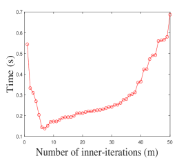
(a)

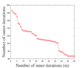
(b)

Figure 1: The computation time and number of outer-iterations of Algorithm 3 for the two-component data with different inner-iterations ($m$).

5.2 Experiments on real data

In this subsection, we utilize two groups of real chemical data, including two-component data ($32\times 39\times 15$) in [29] and macrocephalae rhizoma data ($52\times 214\times\ 16$), to evaluate the performance of various algorithms.

5.2.1 Two-component data

This data contains two components and exhibits background drift, so it can be treated as containing three components. We select the initial number of components as $R=\{3,5,7\}$. The RMSEP values and computation time are shown in Table 1. Figure 2 illustrates the real concentration profiles and the calculated relative concentration profiles resolved by different methods with $R=5$, corresponding to $\mathbf{A}^{(3)}$. Additionally, the change in the number of nonzero columns of $\mathbf{A}^{(3)}$ over the out-iterations is presented in Figure 3.

Table 1: Comparison of computation time (s) and root mean square error of prediction (RMSEP) of different methods for two-component data with $R=3,5,7$. The best results are highlighted in bold. “-” represents that the components are not separated correctly.

	Algorithm	AIBCD	CP_ALS	ATLD	eDLBCPGD	eDLBCPGD_RR
$R=3$	Time	0.032	0.046	0.021	0.225	0.085
	RMSEP	3.607	3.651	6.154	3.935	3.616
$R=5$	Time	0.073	0.081	0.063	0.239	0.141
	RMSEP	-	-	5.913	3.697	3.681
$R=7$	Time	0.089	0.096	0.095	0.361	0.127
	RMSEP	-	-	6.326	3.692	3.678

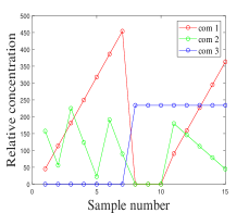
(a)

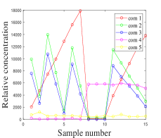
(b)

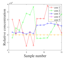
(c)

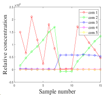
(d)

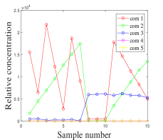
(e)

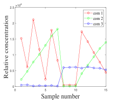
(f)

Figure 2: Analytical results with $R=5$ for the two-component data. Real concentration profiles (a) and relative concentration profiles resolved by (b) AIBCD, (c) CP_ALS, (d) ATLD, (e) eDLBCPGD, and (f) eDLBCPGD_RR, respectively.

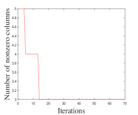
(a)

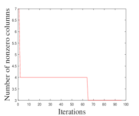
(b)

Figure 3: The number of nonzero columns of the factor matrix $\mathbf{A}^{(3)}$ concerning the iteration numbers.

Table 1 shows that AIBCD and CP_ALS fail to achieve accurate separation when the number of components is overestimated, whereas our proposed methods still exhibit satisfactory results. Although ATLD provides the fastest computational time and obtains correct separation, it yields unsatisfactory RMSEP values and lacks robust theoretical guarantees. Further comparison of eDLBCPGD_RR with eDLBCPGD shows that eDLBCPGD_RR requires less computation time, highlighting the effectiveness of the rank reduction strategy. Figure 2 shows that when $R=5$, only our proposed methods consistently separate exactly three components, underscoring the advantage of incorporating the group sparsity term. Moreover, Figure 3 reports that the number of nonzero columns of $\mathbf{A}^{(3)}$ decreases and eventually stabilizes over the out-iterations. This observation further supports the viability of the rank reduction strategy.

5.2.2 Macrocephalae rhizoma data

The macrocephalae rhizoma data contains three components, and we select the initial number of components as $R=\{3,5,7\}$. The RMSEP values and computation time are reported in Table 2. Figure 4 displays the real concentration profiles and the relative profiles resolved by different methods with $R=7$, corresponding to $\mathbf{A}^{(3)}$. Figure 5 presents the real chromatographic profiles and the normalized chromatographic profiles resolved by different methods with $R=7$, corresponding to $\mathbf{A}^{(1)}$. Figure 6 shows the real spectra profiles and the normalized spectra profiles resolved by different methods with $R=7$, corresponding to $\mathbf{A}^{(2)}$. In Figure 5 and Figure 6, we only show the chromatographic and spectra profiles of the nonzero components resolved by eDLBCPGD.

Table 2: Comparison of computation time (s) and root mean square error of prediction (RMSEP) of different methods for the Macrocephalae rhizoma data with $R=3,5,7$. The best results are highlighted in bold. “-” represents that the components are not separated correctly.

	Algorithm	AIBCD	CP_ALS	ATLD	eDLBCPGD	eDLBCPGD_RR
$R=3$	Time	0.022	0.023	0.113	0.075	0.041
	RMSEP	1.910e-4	6.320e-4	1.950e-4	1.610e-4	1.730e-4
$R=7$	Time	0.037	0.043	0.092	0.112	0.053
	RMSEP	-	-	-	1.590e-4	1.320e-4
$R=5$	Time	0.067	0.113	0.163	0.141	0.093
	RMSEP	-	-	-	2.010e-4	1.060e-4

(a)

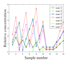
(b)

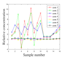
(c)

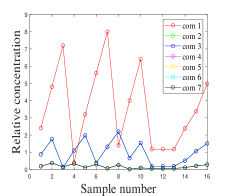
(d)

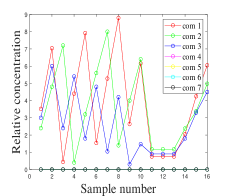
(e)

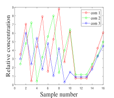
(f)

Figure 4: Analytical results with $R=7$ for the macrocephalae rhizoma data. Real concentration profiles (a) and relative concentration profiles resolved by (b) AIBCD, (c) CP_ALS, (d) ATLD, (e) eDLBCPGD, and (f) eDLBCPGD_RR, respectively.

(a)

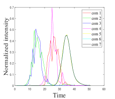
(b)

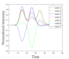
(c)

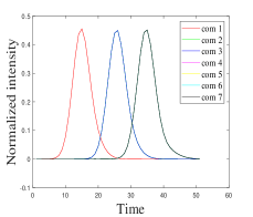
(d)

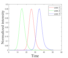
(e)

(f)

Figure 5: Analytical results with $R=7$ for the macrocephalae rhizoma data. Real chromatographic profiles (a) and normalized chromatographic profiles resolved by (b) AIBCD, (c) CP_ALS, (d) ATLD, (e) eDLBCPGD, and (f) eDLBCPGD_RR, respectively.

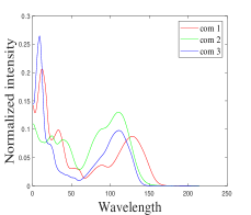
(a)

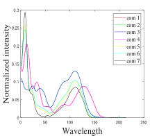
(b)

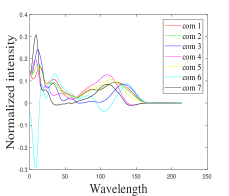
(c)

(d)

(e)

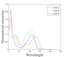
(f)

Figure 6: Analytical results with $R=7$ for the macrocephalae rhizoma data. Real spectra profiles (a) and normalized spectra profiles resolved by (b) AIBCD, (c) CP_ALS, (d) ATLD, (e) eDLBCPGD, and (f) eDLBCPGD_RR, respectively.

As shown in Table 2, only our proposed methods can achieve satisfactory RMSEP when the initial number of components is set to $5$ and $7$. Furthermore, the performance of our proposed methods is comparable to other methods when the initial number of components is accurate. These findings highlight the effectiveness and robustness of our proposed methods. The eDLBCPGD_RR algorithm demonstrates reduced computational time compared to eDLBCPGD, validating the efficiency of the rank reduction strategy. Figure 4, Figure 5, and Figure 6 illustrate that our methods can accurately recover accurate concentration profiles, chromatographic profiles, and spectra profiles with $R=7$, whereas other methods fail to do so. In particular, although ATLD can obtain the spectra of the components, it divides the concentration of a component into equal parts.

6 Conclusions

Most existing CP decomposition-based models and algorithms typically require the accurate estimation of the CP rank, which is a challenging task. To address this challenge, in this paper, we establish the equivalence between the CP rank and the minimization of the group sparsity on any of the factor matrices under the unit length constraints on the columns of the others. Based on this theoretical foundation, we develop a regularized CP decomposition model to obtain a rank CP decomposition of a given tensor. To solve this model, we introduce a double-loop block-coordinate proximal gradient descent algorithm with extrapolation and provide the convergence analysis. Furthermore, based on the proof that the nonzero columns of $\mathbf{A}^{(N)}$ remain unchanged after a certain number of iterations, we develop a rank reduction strategy to reduce the computational complexity. Finally, we apply the proposed model and algorithms to the component separation problem in chemometrics. Numerical experiments conducted on real data demonstrate that our proposed methods can find the optimal solutions even when the initial number of components is overestimated, highlighting the robustness and effectiveness of our approach.

References

- [1] E. Acar and B. Yener. Unsupervised multiway data analysis: A literature survey. IEEE Transactions on Knowledge and Data Engineering, 21(1):6–20, January 2009.
- [2] Casey Battaglino, Grey Ballard, and Tamara G. Kolda. A practical randomized CP tensor decomposition. SIAM Journal on Matrix Analysis and Applications, 39(2):876–901, January 2018.
- [3] Jérôme Bolte, Shoham Sabach, and Marc Teboulle. Proximal alternating linearized minimization for nonconvex and nonsmooth problems. Mathematical Programming, 146(1-2):459–494, 2014.
- [4] J Douglas Carroll and Jih-Jie Chang. Analysis of individual differences in multidimensional scaling via an n-way generalization of “Eckart-Young” decomposition. Psychometrika, 35(3):283–319, 1970.
- [5] Andrzej Cichocki, Namgil Lee, Ivan Oseledets, Anh-Huy Phan, Qibin Zhao, and Danilo P. Mandic. Tensor networks for dimensionality reduction and large-scale optimization: Part 1 low-rank tensor decompositions. Foundations and Trends® in Machine Learning, 9(4–5):249–429, 2016.
- [6] Andrzej Cichocki, Namgil Lee, Ivan Oseledets, Anh-Huy Phan, Qibin Zhao, Masashi Sugiyama, and Danilo P. Mandic. Tensor networks for dimensionality reduction and large-scale optimization: Part 2 applications and future perspectives. Foundations and Trends® in Machine Learning, 9(6):249–429, 2017.
- [7] Fengyu Cong, Qiu-Hua Lin, Li-Dan Kuang, Xiao-Feng Gong, Piia Astikainen, and Tapani Ristaniemi. Tensor decomposition of eeg signals: A brief review. Journal of Neuroscience Methods, 248:59–69, June 2015.
- [8] Ian Davidson, Sean Gilpin, Owen Carmichael, and Peter Walker. Network discovery via constrained tensor analysis of fmri data. In Proceedings of the 19th ACM SIGKDD international conference on Knowledge discovery and data mining, KDD’ 13. ACM, August 2013.
- [9] Ignat Domanov and Lieven De Lathauwer. On the uniqueness of the canonical polyadic decomposition of third-order tensors—part ii: Uniqueness of the overall decomposition. SIAM Journal on Matrix Analysis and Applications, 34(3):876–903, 2013.
- [10] Richard A. Harshman. Foundations of the parafac procedure: Models and conditions for an ”explanatory” multi-model factor analysis. 1970.
- [11] F. L. Hitchcock. The expression of a tensor or a polyadic as a sum of products. Journal of Mathematics and Physics, 6:164–189, 1927.
- [12] Johan Håstad. Tensor rank is NP-complete. Journal of Algorithms, 11(4):644–654, December 1990.
- [13] Tamara G Kolda and Brett W Bader. Tensor decompositions and applications. SIAM review, 51(3):455–500, 2009.
- [14] Joseph B Kruskal. Three-way arrays: rank and uniqueness of trilinear decompositions, with application to arithmetic complexity and statistics. Linear algebra and its applications, 18(2):95–138, 1977.
- [15] Joseph B. Kruskal. Rank, decomposition, and uniqueness for 3-way and N-way arrays. 1989.
- [16] Brett W. Larsen and Tamara G. Kolda. Practical leverage-based sampling for low-rank tensor decomposition. SIAM Journal on Matrix Analysis and Applications, 43(3):1488–1517, August 2022.
- [17] Lea Lenhardt, Rasmus Bro, Ivana Zeković, Tatjana Dramićanin, and Miroslav D. Dramićanin. Fluorescence spectroscopy coupled with parafac and pls da for characterization and classification of honey. Food Chemistry, 175:284–291, May 2015.
- [18] Makoto Nakatsuji, Qingpeng Zhang, Xiaohui Lu, Bassem Makni, and James A. Hendler. Semantic social network analysis by cross-domain tensor factorization. IEEE Transactions on Computational Social Systems, 4(4):207–217, December 2017.
- [19] Dimitri Nion and Nicholas D. Sidiropoulos. Tensor algebra and multidimensional harmonic retrieval in signal processing for mimo radar. IEEE Transactions on Signal Processing, 58(11):5693–5705, November 2010.
- [20] R Tyrrell Rockafellar and Roger J-B Wets. Variational analysis, volume 317. Springer Science & Business Media, 2009.
- [21] N.D. Sidiropoulos, G.B. Giannakis, and R. Bro. Blind PARAFAC receivers for DS-CDMA systems. IEEE Transactions on Signal Processing, 48(3):810–823, March 2000.
- [22] Nicholas D Sidiropoulos and Rasmus Bro. On the uniqueness of multilinear decomposition of n-way arrays. Journal of Chemometrics: A Journal of the Chemometrics Society, 14(3):229–239, 2000.
- [23] Marco Signoretto, Quoc Tran Dinh, Lieven De Lathauwer, and Johan A. K. Suykens. Learning with tensors: a framework based on convex optimization and spectral regularization. Machine Learning, 94(3):303–351, May 2013.
- [24] Ravendra Singh. Implementation of control system into continuous pharmaceutical manufacturing pilot plant (powder to tablet). In Computer Aided Chemical Engineering, volume 41, pages 447–469. Elsevier, 2018.
- [25] Le Sun, Feiyang Wu, Tianming Zhan, Wei Liu, Jin Wang, and Byeungwoo Jeon. Weighted nonlocal low-rank tensor decomposition method for sparse unmixing of hyperspectral images. IEEE Journal of Selected Topics in Applied Earth Observations and Remote Sensing, 13:1174–1188, 2020.
- [26] DeQing Wang and FengYu Cong. An inexact alternating proximal gradient algorithm for nonnegative CP tensor decomposition. Science China Technological Sciences, 64(9):1893–1906, July 2021.
- [27] Qingsong Wang, Chunfeng Cui, and Deren Han. Accelerated doubly stochastic gradient descent for tensor CP decomposition. Journal of Optimization Theory and Applications, 197(2):665–704, March 2023.
- [28] Qingsong Wang, Zehui Liu, Chunfeng Cui, and Deren Han. Inertial accelerated SGD algorithms for solving large-scale lower-rank tensor CP decomposition problems. Journal of Computational and Applied Mathematics, 423:114948, May 2023.
- [29] Tong Wang, Qian Liu, Wan-Jun Long, An-Qi Chen, Hai-Long Wu, and Ru-Qin Yu. A chemometric comparison of different models in fluorescence analysis of dabigatran etexilate and dabigatran. Spectrochimica Acta Part A: Molecular and Biomolecular Spectroscopy, 246:118988, 2021.
- [30] Zihao Wang and Minru Bai. An inexactly accelerated algorithm for nonnegative tensor CP decomposition with the column unit constraints. Computational Optimization and Applications, pages 1–40, 2024.
- [31] Hai-Long Wu, Masami Shibukawa, and Koichi Oguma. An alternating trilinear decomposition algorithm with application to calibration of HPLC–DAD for simultaneous determination of overlapped chlorinated aromatic hydrocarbons. Journal of Chemometrics: A Journal of the Chemometrics Society, 12(1):1–26, 1998.
- [32] Hai-Long Wu, Tong Wang, and Ru-Qin Yu. Chapter 22 - new application of trilinear decomposition model: Theory, data processing, and classical quantitative applications. In Alejandro C. Olivieri, Graciela M. Escandar, Héctor C. Goicoechea, and Arsenio Muñoz de la Peña, editors, Fundamentals and Applications of Multiway Data Analysis, volume 33 of Data Handling in Science and Technology, pages 549–635. Elsevier, 2024.
- [33] Hai-Long Wu, Tong Wang, and Ru-Qin Yu. Chapter 23 - new application of trilinear decomposition model: New quantitative and qualitative applications. In Alejandro C. Olivieri, Graciela M. Escandar, Héctor C. Goicoechea, and Arsenio Muñoz de la Peña, editors, Fundamentals and Applications of Multiway Data Analysis, volume 33 of Data Handling in Science and Technology, pages 637–670. Elsevier, 2024.
- [34] Yang Xu, Zebin Wu, Jocelyn Chanussot, and Zhihui Wei. Hyperspectral computational imaging via collaborative Tucker3 tensor decomposition. IEEE Transactions on Circuits and Systems for Video Technology, 31(1):98–111, January 2021.
- [35] Yuning Yang. The epsilon-alternating least squares for orthogonal low-rank tensor approximation and its global convergence. SIAM Journal on Matrix Analysis and Applications, 41(4):1797–1825, January 2020.