Abstract

It is known for long that the observed mass surface density of cored dark matter (DM) halos is approximately constant, independently of the galaxy mass (i.e., $\rho_{c}r_{c}\simeq{\rm constant}$, with $\rho_{c}$ and $r_{c}$ the central volume density and the radius of the core, respectively). Here we review the evidence supporting this empirical fact as well as its theoretical interpretation. It seems to be an emergent law resulting from the concentration-halo mass relation predicted by the current cosmological model, where the DM is made of collisionless cold DM particles (CDM). We argue that the prediction $\rho_{c}r_{c}\simeq{\rm constant}$ is not specific to this particular model of DM but holds for any other DM model (e.g., self-interacting) or process (e.g., stellar or AGN feedback) that redistributes the DM within halos conserving its CDM mass. In addition, the fact that $\rho_{c}r_{c}\simeq{\rm constant}$ is shown to allow the estimate of the core DM mass and baryon fraction from stellar photometry alone, particularly useful when the observationally-expensive conventional spectroscopic techniques are unfeasible.

1 1 0 https://doi.org/ Implications of the intriguing constant inner mass surface density observed in dark matter halos Constant mass surface density in dark matter halos Jorge Sánchez Almeida^1,2*0000-0003-1123-6003 Sánchez Almeida, J. Correspondence: jos@iac.es

1 Introduction

The shape of the dark matter (DM) halos hosting galaxies can be inferred from rotation curves or other kinematical measurements (e.g., Persic et al., 1996; Oh et al., 2015; Salucci, 2019). The resulting DM radial profiles often show an inner plateau or core characterized by a central mass density $\rho_{c}$ and a core radius $r_{c}$ which combined happen to yield a surface density approximately constant,

$$\rho_{c}r_{c}\simeq{\rm constant},$$ (1)

a property observed to hold in a wide range of halo masses $M_{h}$, between $10^{9}$ and $10^{12}\,M_{\odot}$ Burkert (1995); Salucci and Burkert (2000); Spano et al. (2008); Donato et al. (2009); Salucci et al. (2012); Saburova and Del Popolo (2014); Burkert (2015); Kormendy and Freeman (2016); Di Paolo et al. (2019) (actual values and details will be given in Sect. 2 and Appendix A). Originally, it was a rather surprising result Burkert (1995) but nowadays it is interpreted in the literature as an emergent law caused by the well known relation between halo mass and concentration arising in collisionless cold dark matter (CDM) numerical simulations Lin and Loeb (2016); Burkert (2020); Kaneda et al. (2024). In CDM-only simulations, the CDM halos do not have cores. They follow the canonical NFW profiles Navarro et al. (1997) or the Einasto profiles Wang et al. (2020), with a pronounced inner cusp where the density grows continuously toward the center of the halo. Thus, an additional physical process must operate to transform the cuspy CDM halos into cored halos, conserving the original DM mass. This transformation is usually assumed to be driven by baryon processes like star-formation feedback, AGN feedback, or galaxy mergers, which shuffle around the baryonic mass, thus changing the overall gravitational potential and affecting the distribution of CDM. CDM cores appear in model galaxies formed in full hydrodynamical cosmological numerical simulations (e.g., Governato et al., 2010; Pontzen and Governato, 2014; Lazar et al., 2020). Thus, Eq. (1) is often regarded as a support for CDM (Kaneda et al., 2024, and references therein). However, the formation of cores in DM halos can be driven by any physical processes that thermalizes the DM distribution Plastino and Plastino (1993); Sánchez Almeida et al. (2020). They will also render Eq. (1), provided the process just redistributes the available mass, not changing much the relation between halo mass and concentration set by the cosmological initial conditions (Sect. 5.1).

The purpose of this work is to review the observational evidence for Eq. (1) as well as the theory behind it. The interpretation can be pinned down to the relation between the mass of a DM halo and its age of formation (Sect. 5.1), which is set by cosmology and to a lesser extent by details on the nature of DM. As a spin-off, we demonstrate how Eq. (1) can be used to estimate the mass in the DM halo of a galaxy based solely on the distribution of its stars. The approach is based on the fact that dwarf galaxies also tend to show a central plateau or core in the stellar distribution (e.g., Carlsten et al., 2021; Montes et al., 2024). The radii of the stellar and the DM cores are expected to scale with each other Sánchez Almeida et al. (2024a, b). We worked out the relation between the core radius of the stellar distribution and the DM mass.

The paper is organized as follows: Section 2 collects observational evidence for Eq. (1). Section 3 works out the explanation of Eq. (1) within CDM. Section 4 compares the observations in Sect. 2 with the theory in Sect. 3. Based on Eq. (4), Sect. 5 writes down a semi-empirical relation between the stellar core radius and DM halo mass. It also shows that the stellar mass surface density is a proxy for the baryon fraction in the center of a galaxy. Ready to use relations are given in Eqs. (25) and (26). Section 6 summarizes the main conclusions in the work.

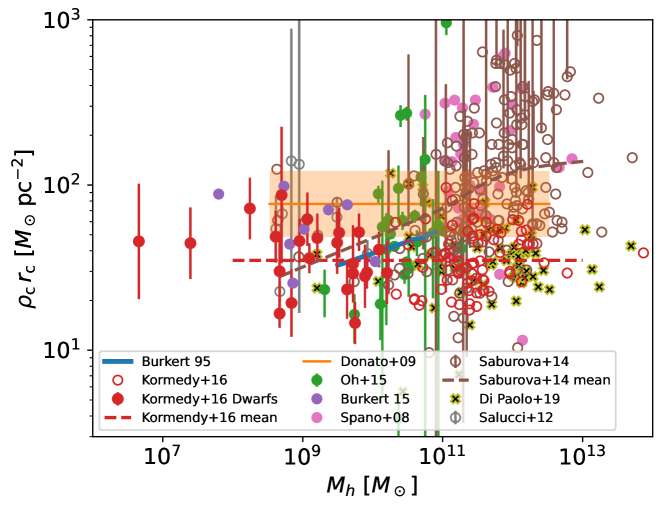
Figure 1: Compilation of values of $\rho_{c}r_{c}$ from the literature as a function of the DM halo mass of the galaxy ($M_{h}$). Details on the references and the processing are given in Appendix A. A version of this figure but showing the same eight orders of magnitude range for abscissae and ordinates is shown in Fig. 12. References: Burkert 95 Burkert (1995), Kormendy+16 Kormendy and Freeman (2016), Donato+09 Donato et al. (2009), Oh+15 Oh et al. (2015), Burkert 15 Burkert (2015), Spano+08 Spano et al. (2008), Saburova+14 Saburova and Del Popolo (2014), Di Paolo+19 Di Paolo et al. (2019), and Salucci+12 Salucci et al. (2012). The inset gives a color and symbol code which is the same used in Figs. 3, 4, and 5.

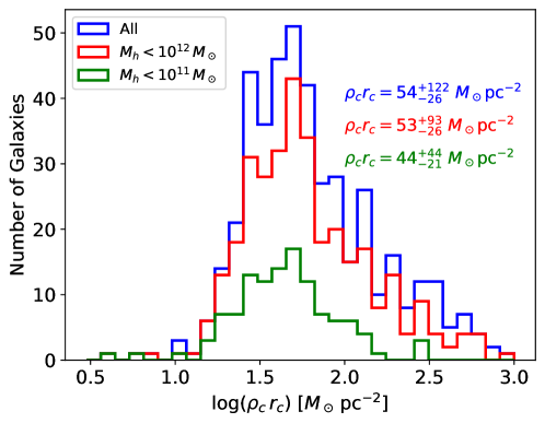
Figure 2: Histograms with the distribution of $\rho_{c}r_{c}$ represented in Fig. 1 and detailed in Appendix A. We show three different selections: all galaxies (the blue line), galaxies with halo masses $M_{h}<10^{12}\,M_{\odot}$ (the red line), and galaxies with $M_{h}<10^{11}\,M_{\odot}$ (the green line). The last one is representative of dwarf galaxies. The inset gives the median of each distribution, as well as the range between percentiles 15.9 % and 84.1 % (i.e., median $\pm 1\,$sigma).

2 Observations supporting Eq. (1)

As we point out in Sect. 1, the product $\rho_{c}r_{c}$ is approximately constant over a large range in galaxy mass. To emphasize the existing evidence, we have compiled a number of relations between $\rho_{c}r_{c}$ and $M_{h}$ from the literature. They are based on uneven measurements prone to bias, including the determination of the DM halo mass of a galaxy and the definition of core radius. However, the conclusion is clear, with the different independent determinations agreeing within error bars. The result of the compilation is shown in Figs. 1 – 5. Details of how the individual works were interpreted to construct the figures are given in Appendix A. In particular, here and throughout the paper, we assume the core radius to be the radius where the density drops to half the central value,

$$\rho(r_{c})=\rho_{c}/2,$$ (2)

with $\rho_{c}=\rho(0)$. This definition is not universally used and so often the radii quoted in the original reference have to be transformed to our definition, as detailed in Appendix A.

Figure 1 gives the scatter plot of $\rho_{c}r_{c}$ versus $M_{h}$. The extreme values are likely unreliable but it is clear that the product $\rho_{c}r_{c}$ tends to be constant, at least for $M_{h}<10^{11}M_{\odot}$. This fact is better appreciated in Fig. 12, which is identical to Fig. 1 but with the vertical axis spanning the same eight orders of magnitude of the horizontal axis corresponding to the DM halo masses. Histograms with the values of $\rho_{c}r_{c}$ in Fig. 1 are shown in Fig. 2. They include all the observed values (the blue line), when $M_{h}<10^{12}M_{\odot}$ (the red line), and when $M_{h}<10^{11}M_{\odot}$ (the green line). An inset in the figure also gives the median and the 1-sigma percentiles of the distributions (i.e., 50 %, 15.9 % and 84.1 %) which correspond to

$$\rho_{c}r_{c}=44^{+44}_{-21}\,M_{\odot}\,{\rm pc}^{-2},$$ (3)

when $M_{h}<10^{11}M_{\odot}$, a limit representative of dwarf galaxies. We note that the used $r_{c}$, as set by Eq. (2), is typically a factor of two smaller than the core radii commonly defined in the literature. Thus, the surface density in Eq. (3) is fully consistent with a value around $100\,M_{\odot}\,{\rm pc}^{-2}$ often quoted in the literature (see, e.g., Salucci and Burkert (2000); Burkert (2020)). As we explain in Appendix A, the estimate of $M_{h}$ used in Fig. 1 relies on the observed absolute magnitude of the galaxies, assuming a mass-to-light ratio and a relation between stellar mass and DM halo mass as inferred from abundance matching Behroozi et al. (2013). However, the trend for $\rho_{c}r_{c}$ to become constant in dwarf galaxies is already present in the original data; see Fig. 3, where the abscissa are given by the measured absolute magnitude of the galaxy.

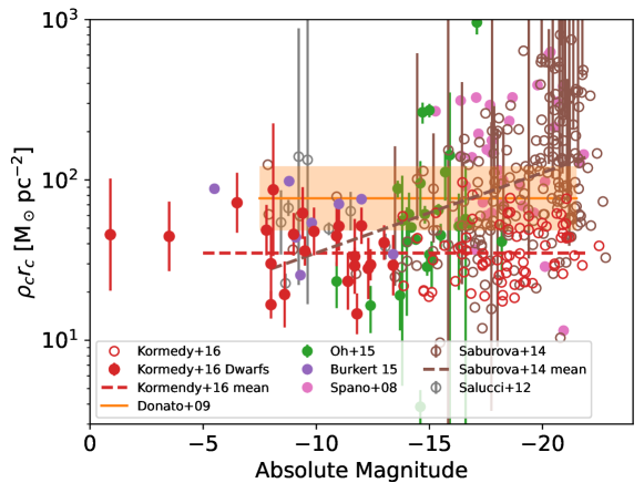
Figure 3: Central DM surface density, $\rho_{c}r_{c}$, as a function of the absolute magnitude of the galaxy, which is the observable employed to estimate the halo masses represented in Fig. 1. The absolute magnitude is $M_{B}$ or $M_{V}$ depending on the galaxy. The inset gives the color and symbol code, which is the same employed in Figs. 1, 4, and 5.

Figure 4 gives $\rho_{c}r_{c}$ (top panel) and $\rho_{c}r_{c}^{3}$ (bottom panel) versus $r_{c}$. Note that the latter gives the DM mass in the core and it scales as $r_{c}^{2}$ following Eq. (3), which is represented in the figure by the gray dashed line. These relations are independent of the uncertainties in $M_{h}$.

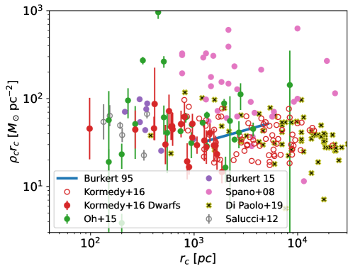
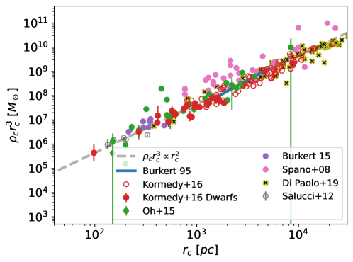
Figure 4: Observed $\rho_{c}r_{c}$ versus $r_{c}$ (top panel) and $\rho_{c}r_{c}^{3}$ versus $r_{c}$ (bottom panel). Note that the latter gives the DM mass in the core and scales as $r_{c}^{2}$ following Eq. (3), which is represented by the gray dashed line. These relations do not depend on the total DM halo mass and can be used to test theoretical explanations bypassing uncertainties in $M_{h}$. The insets give the color and symbol code, used also in Figs. 1, 3, and 5.

Figure 5 gives the relation of $r_{c}$ with $M_{h}$ (top panel) and $\rho_{c}$ with $M_{h}$ (bottom panel). The correlation happens to be very clear in both cases. The larger the mass, the larger the radius and the smaller the density. In order to guide the eye, the figure includes power laws as $r_{c}\propto M_{h}^{0.4}$ (top panel) and $\rho_{c}\propto M_{h}^{-0.4}$ (bottom panel), which approximately describe the observed trends. Note that combined, these power laws render Eq. (1).

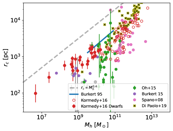
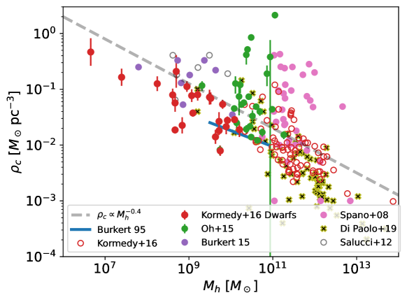
Figure 5: Top panel: core radius $r_{c}$ versus DM halo mass $M_{h}$. The dashed line is a power law with exponent $+0.4$ and has been included to guide the eye. Bottom panel: central DM density $\rho_{c}$ versus DM halo mass. This time the dashed line is a power law with exponent $-0.4$. The insets give the color and symbol code, which is the same used in Figs. 1, 3, and 4.

3 Theory: cores resulting from redistributing collisionless cold dark matter halos

If the DM was collisionless CDM and if there were no baryons, then the distribution of DM within each halo would approximately follow the iconic NFW profile Navarro et al. (1997),

$$\rho_{\rm NFW}(r)=\frac{\rho_{s}}{(r/r_{s})\,(1+r/r_{s})^{2}},$$ (4)

describing the variation with radius $r$ of the DM volume density $\rho_{\rm NFW}(r)$. The parameters $r_{s}$ and $\rho_{s}$ stand for a scaling radius and a scaling density, respectively. The mass available to form any DM halo today is provided by the initial conditions set by cosmology (see Sect. 5.1). It would be the same independently of whether a physical process redistributes this mass in a different mass density profile. Probably, the most general such process is the thermalization the DM distribution. In this case, one expects the formation of a core with a generic polytropic shape, characteristic of self-gravitating systems reaching thermodynamic equilibrium Plastino and Plastino (1993); Sánchez Almeida et al. (2020); Sánchez Almeida (2022). For analytic simplicity, we assume the $m=5$ polytrope (best known as Schuster-Plummer profile), but the core of all polytropes has virtually the same shape (e.g., Sánchez Almeida, 2022). In this case,

$$\rho_{5}(r)=\frac{\rho_{c}}{\left[1+(r/b)^{2}\right]^{5/2}},$$ (5)

with $\rho_{c}$ the central density and $b$ a length scale setting the core radius defined as in Eq. (1),

$$r_{c}=b\times\sqrt{2^{2/5}-1}\simeq b\times 0.56525\dots.$$ (6)

Thus, the new density profile resulting from the core formation is a piecewise function defined as Eq. (5) in the core, Eq. (4) in the outskirts, and continuous in the matching radius $r_{m}$,

$$\rho(r)=\begin{cases}\rho_{5}(r),&{\rm when~~}r<r_{m},\\ \rho_{5}(r_{m})=\rho_{\rm NFW}(r_{m}),&{\rm when~~}r=r_{m},\\ \rho_{\rm NFW}(r),&{\rm when~~}r>r_{m}.\end{cases}$$ (7)

In addition, to conserve mass,

$$\int_{0}^{\infty}\rho(r)\,r^{2}\,dr=\int_{0}^{\infty}\rho_{\rm NFW}(r)\,r^{2}\,dr,$$ (8)

which, considering Eq. (7), renders

$$\int_{0}^{r_{m}}\rho_{5}(r)\,r^{2}\,dr=\int_{0}^{r_{m}}\rho_{\rm NFW}(r)\,r^{2}\,dr.$$ (9)

Examples of these cored DM profiles with NFW outskirts are given in Fig. 6. This kind of piecewise shape has already been used in the literature (e.g., Robertson et al., 2021; Sánchez Almeida and Trujillo, 2021).

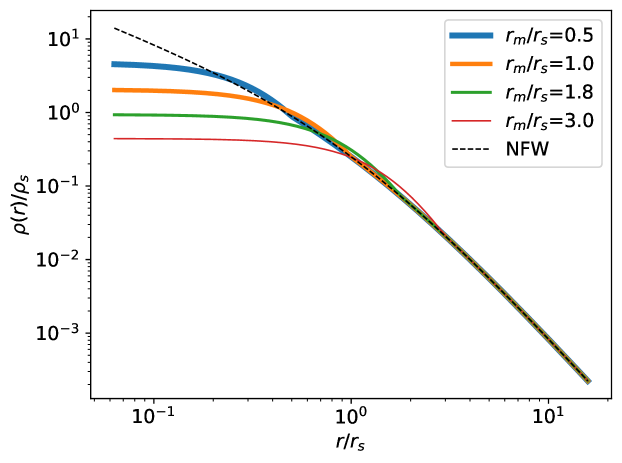
Figure 6: Piecewise density profiles with an inner core ($m=5$ polytrope; $\rho_{5}$ in Eq. [5]) and an outer NFW profile ($\rho_{\rm NFW}$; Eq. [4]). The two pieces coincide at the matching radius $r_{m}$, $\rho_{5}(r_{m})=\rho_{\rm NFW}(r_{m})$, and the total mass is the total mass of $\rho_{\rm NFW}(r)$ (Eq. [8]). The full NFW profile is shown as a black dashed line whereas profiles for different matching radii are shown with different colors as indicated in the inset.

Equations (7) and (9) provide a mapping between the parameters of the NFW profile ($\rho_{s}$ and $r_{s}$) and the parameters defining the core ($\rho_{c}$ and $b$). The continuity at $r_{m}$ forces

$$\frac{\rho_{c}}{(1+(r_{m}/b)^{2})^{5/2}}=\frac{\rho_{s}}{(r_{m}/r_{s})(1+r_{m}/r_{s})^{2}},$$ (10)

whereas mass conservation, Eq. (9), leads to

$$\rho_{c}\,r_{m}^{3}\,\frac{1}{3\,[1+(r_{m}/b)^{2}]^{3/2}}=\rho_{s}\,r_{s}^{3}\,\left[\ln(1+\frac{r_{m}}{r_{s}})-\frac{r_{m}/r_{s}}{1+r_{m}/r_{s}}\right].$$ (11)

After some algrebra, Eqs. (10) and (11) render,

$$1+\left(\frac{r_{m}/r_{s}}{b/r_{s}}\right)^{2}=\frac{3\,(1+r_{m}/r_{s})^{2}}{(r_{m}/r_{s})^{2}}\,\left[\ln(1+\frac{r_{m}}{r_{s}})-\frac{r_{m}/r_{s}}{1+r_{m}/r_{s}}\right],$$ (12)

and

$$\frac{\rho_{c}\,b^{3}}{\rho_{s}\,r_{s}^{3}}=\frac{3\,[1+(r_{m}/b)^{2}]^{3/2}}{(r_{m}/b)^{3}}\,\left[\ln(1+\frac{r_{m}}{r_{s}})-\frac{r_{m}/r_{s}}{1+r_{m}/r_{s}}\right].$$ (13)

We note that once $r_{m}/r_{s}$ is set (i.e., the radius of match in units of $r_{s}$; see Eq. [7]), Eqs. (12) and (13) give the full density profile. Equation (12) provides $b/r_{s}$, which can be used in Eq. (13) to compute $\rho_{c}/\rho_{s}$, and then $\rho(r)/\rho_{s}$. This is the procedure followed to compute the densities shown in Fig. 6.

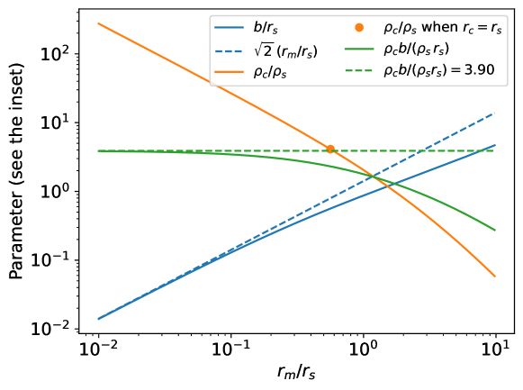
Figure 7: Dependence on $r_{m}/r_{s}$ of $b/r_{s}$, $\rho_{c}/\rho_{s}$, and $\rho_{c}b/(\rho_{s}r_{s})$ as given by Eqs. (12) and (13). The solid lines show the actual variation whereas the dashed lines correspond to the dependence when the transition radius $r_{m}\ll r_{s}$ (Eqs. [15] and [16]). The orange symbol points out when $r_{c}=r_{s}$, which has $r_{m}/r_{s}\simeq 0.56$ and $\rho_{c}/\rho_{s}\simeq 4.11$.

Figure 7 shows the dependence on $r_{m}/r_{s}$ for $b/r_{s}$, $\rho_{c}/\rho_{s}$, and $\rho_{c}b/(\rho_{s}r_{s})$. We note that for $r_{m}\lesssim r_{s}$, $b\sim r_{s}$ and $\rho_{c}b\sim\rho_{s}r_{s}$. These dependences are easy to distill from the above equations in the limit $r_{m}\ll r_{s}$. In this case,

$$\ln(1+\frac{r_{m}}{r_{s}})-\frac{r_{m}/r_{s}}{1+r_{m}/r_{s}}\simeq\frac{(r_{m}/r_{s})^{2}}{2},$$ (14)

so that Eq. (12) renders,

$$b/r_{s}\simeq\sqrt{2}\,(r_{m}/r_{s}).$$ (15)

Similarly, Eq. (13) plus Eq. (15) render

$$\rho_{c}b\simeq\rho_{s}r_{s}\,(3/2)^{2}\sqrt{3}=\rho_{s}r_{s}\times 3.89711\dots.$$ (16)

When $r_{m}=r_{s}$ (i.e., when the matching radius coincides with the characteristic radius defining the NFW profile) then things simplify even further so that,

$$\frac{\rho_{c}r_{c}}{\rho_{s}r_{s}}\simeq 1.0068\dots,$$ (17)

where we have used Eq. (6) to transform $b$ into $r_{c}$ (details in Appendix B).

The NFW halos are given setting $\rho_{s}$ and $r_{s}$. In the context of CDM, these two variables are often replaced by the concentration $c$ and the halo mass $M_{h}$, so that,

$$\rho_{s}=\frac{200\,c^{3}\,\rho_{crit}}{3\big{[}\ln(1+c)-c/(1+c)\big{]}},$$ (18)

and,

$$r_{s}^{3}=\frac{3\,M_{h}}{800\pi\,\rho_{crit}\,c^{3}}.$$ (19)

The symbol $\rho_{crit}$ stands for the critical density of the Universe. Pieced together, Eqs. (18) and (19) render the dependence of the product $\rho_{s}r_{s}$ on $c$ and $M_{h}$,

$$\rho_{s}r_{s}=\frac{10}{3}\,\left(\frac{30}{\pi}\right)^{1/3}\,\frac{\rho_{crit}^{2/3}\,c^{2}\,M_{h}^{1/3}}{\ln(1+c)-c/(1+c)},$$ (20)

a relation that can be found already in the literature (e.g., Lin and Loeb, 2016).

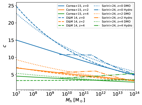
Figure 8: Relation between concentration $c$ and halo mass $M_{h}$ inferred from various CDM only simulations. The three papers cited in the inset are D&M 14 Dutton and Macciò (2014), Correa+15 Correa et al. (2015), and Sorini+24 Sorini et al. (2024). For reference, we also show a relation obtained when baryon feedback is self-consistently treated in the simulation (the dotted dashed lines). Different redshifts ($z$) are included with different colors, whereas the type of line encodes the actual reference (see the inset).

The numerical simulations of CDM predict a relation between $c$ and $M_{h}$, which varies with redshift and is quite tight for $M_{h}>10^{10}\,M_{\odot}$ to become looser at smaller halo mass Dutton and Macciò (2014); Correa et al. (2015); Sorini et al. (2024). Examples of this relation are given in Fig. 8, where we note that the range of variation of $c$ is quite moderate, changing only by a factor of three for halos varying by seven orders of magnitude in mass, from $10^{7}$ to $10^{14}~M_{\odot}$; see the blue lines in Fig. 8. Thus, considering $c$ constant, the dependence of $\rho_{s}r_{s}$ on halo mass predicted by Eq. (20) is quite mild as it scales as $M_{h}^{1/3}$. This fact, together with the approximate equivalence given by Eqs. (6) and (16), indicates that the predicted $\rho_{c}r_{c}$ is expected to vary little with halo mass,

$$\rho_{c}r_{c}\propto\rho_{c}b\propto\rho_{s}r_{s}\propto M_{h}^{1/3},$$ (21)

as it is indeed observed (Sect. 2).

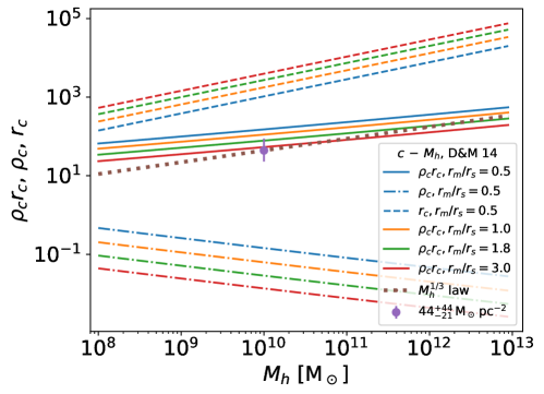
Figure 9: Predicted variation of the central mass surface density $\rho_{c}r_{c}$ as a function of $M_{h}$ for various $r_{m}/r_{s}$ assuming the $c$–$M_{h}$ relation at redshift zero given in Dutton and Macciò (2014) (the solid lines). The figure also includes the variation of $r_{c}$ (the dashed lines) and $\rho_{c}$ (the dashed-dotted lines) to emphasize how the increase of $r_{c}$ with increasing $M_{h}$ is partly balanced by the decrease of $\rho_{c}$ to produce a fairly constant $\rho_{c}r_{c}$. The dotted line shows the approximate dependence of $\rho_{c}r_{c}$ on $M_{h}$ to be expected if $c$ were constant (Eq. [21]). This power law dependence has been anchored to the observed $\rho_{c}r_{c}$ (Eq. [3]) assumed to represent $M_{h}\sim 10^{10}~M_{\odot}$. The core density $\rho_{c}$ and core radius $r_{c}$ are given in units of $M_{\odot}\,{\rm pc}^{-3}$ and ${\rm pc}$, respectively.

The equations above yield $\rho_{c}r_{c}$ as a function of $M_{h}$. The algorithm to compute it is: (1) set $r_{m}/r_{s}$, (2) get $c$ of $M_{h}$ from the literature (Fig. 8), (3) get $\rho_{s}$ and $r_{s}$ as a function of $M_{h}$ from Eqs. (18) and (19), (4) get $b/r_{s}$ of $M_{h}$ from $r_{s}$ and Eq. (12), (5) get $\rho_{c}/\rho_{s}$ of $M_{h}$ from $b/r_{s}$, $r_{m}/r_{s}$, and Eq. (13), (6) get $r_{c}/b$ from Eq. (6) and, finally, (7) compute

$$\rho_{c}r_{c}=\rho_{s}\times r_{s}\times\frac{b}{r_{s}}\times\frac{\rho_{c}}{\rho_{s}}\times\frac{r_{c}}{b}.$$ (22)

Figure 9 shows the predicted variation of $\rho_{c}r_{c}$ as a function of $M_{h}$ for various $r_{m}/r_{s}$ assuming the $c$–$M_{h}$ relation at redshift zero given in Dutton and Macciò (2014) (the solid lines). Qualitatively, the trends for other $c$–$M_{h}$ relations and redshifts look the same. The figure also includes the variation of $r_{c}$ (the dashed lines) and $\rho_{c}$ (the dashed dotted lines) separately. Note how the increase of $r_{c}$ with $M_{h}$ is partly balanced by the decrease of $\rho_{c}$, leaving a fairly constant $\rho_{c}r_{c}$.

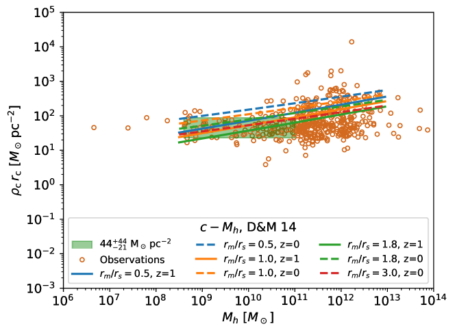
Figure 10: Observed versus predicted $\rho_{c}r_{c}$. The observations are the same as those used in Fig. 1 except that ordinates and abscissae have been forced to span the same eight order of magnitude range. The colored lines represent the theoretical predictions, which depend on the parameter $r_{m}/r_{s}$ and the redshift $z$ from which the $c$–$M_{h}$ relation was taken (see the inset). The range of $\rho_{c}r_{c}$ values for $M_{h}<10^{11}\,M_{\odot}$ given in Eq. (3) is shown as the pale green region.

4 Comparison between observations and theory

Figure 10 shows the observed $\rho_{c}r_{c}$ (the symbols) compared with the prediction using the simple equations worked out in Sect. 3, where the DM cores are assumed to result from the redistribution of mass of the CDM halos. The observed data points in Fig. 10 are those in Fig. 1 but shown in a range spanning the same eight orders of magnitude variation for both $\rho_{c}r_{c}$ and $M_{h}$. This particular scaling evidences how constant $\rho_{c}r_{c}$ is, with the range of values in Eq. (3) highlighted as the pale green region. The colored lines represent the theoretical predictions and they agree well with the observation without any fine tuning. They even reproduce a slight increase of $\rho_{c}r_{c}$ with halo mass, which is probably too large in the theoretical model, although given the observational uncertainties one should not stress this fact further. Note that the prediction depends on the parameter $r_{m}/r_{s}$ and the redshift $z$ from which the relation $c$–$M_{h}$ was taken. The best agreement with observation corresponds to $r_{m}/r_{s}$ between 1 and 2 starting off from halos at $z=0$, and between 0.5 and 1 starting from halos a bit earlier at $z=1$. Figure 10 is based on the theoretical $c$–$M_{h}$ from Dutton and Macciò (2014), but the results are similar for the other theoretical $c$–$M_{h}$ analyzed in Sect. 2 and Figs. 8 and 9.

5 Discussion

Here we analyze the implications of the fair agreement between theory and observation presented in Sect. 4.

5.1 What sets the $c$–$M_{h}$ relation?

Note that so far the answer to the question of what sets $\rho_{c}r_{c}\simeq$ constant is the existence of a $c$–$M_{h}$ relation for the DM halos produced in the $\Lambda$CDM cosmology (see Figs. 8 and 9). Thus, unless we understand in physical terms what sets the $c$–$M_{h}$ relation of the collisionless CDM halos, the above explanation of why $\rho_{c}r_{c}$ is constant sounds circular.

Correa et al. (2015) describe the current understanding in detail, and give a number of relevant references. According to this view, the relation seems to be driven by the inside-out growth of the DM halos combined with the fact that low mass halos collapse first. The build-up of all halos generally consists of an early phase of fast accretion and a late phase where the accretion slows down Zhao et al. (2003); Lu et al. (2006). During the early phase, halos are formed with low concentration, and then the concentration increases during the second phase as the outer halo grows and the mass-accretion rate decreases. The concentration grows during this second phase because the virial radius setting the size of the whole halo increases while $r_{s}$ remains rather constant${}^{\ref{this_footnote}}$. Halos of all masses undergo these two phases, but low mass halos complete the first phase early on and so they show large concentrations at present, whereas the very massive ones are still in the first phase. This process gives rise to the variation predicted by the numerical simulations shown in Fig. 8. Contrary to the low mass halos, the high mass halos show little evolution of the concentration with redshift (or, equivalently, with time). According to this scenario, the actual $c$–$M_{h}$ relation should depend significantly on the cosmological parameters, in particular, on $\sigma_{8}$ that parameterizes the amplitude of the matter density fluctuations in the early Universe, and on $\Omega_{m}$ that quantifies the total amount of matter. The larger $\sigma_{8}$ or $\Omega_{m}$, the earlier the halos assemble and the larger the resulting concentration Correa et al. (2015).

5.2 Relation between DM core mass and stellar core radius

The DM halo mass within the visible stellar core is

$$M_{hc}=\frac{4\pi}{3}\rho_{c}r_{\star c}^{3}=\frac{4\pi g\kappa_{c}}{3}\,r_{\star c}^{2},$$ (23)

with $\kappa_{c}$ the constant $\rho_{c}r_{c}$, $r_{\star c}$ the stellar core radius, and $g=r_{\star c}/r_{c}$. Provided $g\lesssim 1$, Eq. (23) gives the DM mass within the observed stellar core. Even if this is a relationship between the core DM halo mass and the stellar radius, it is encouraging to note that a similar relation is observed to hold between the DM core mass and the DM core radius (Fig. 4), and between the total DM halo mass and the core radius; see the dashed line in Fig. 5, corresponding to $M_{h}\propto r_{c}^{2.5}$. The baryon fraction in the core, defined as

$$f_{bc}=\frac{M_{\star c}}{M_{hc}}=\frac{\rho_{\star c}r_{\star c}}{g\kappa_{c}},$$ (24)

can be inferred from the observed stellar mass surface density, $\rho_{\star c}r_{\star c}$, provided $g$ can be measured or estimated. Thus, if Eq. (1) holds, from the stellar distribution alone one can estimate the DM core mass and the baryon fraction in the core. Using $\kappa_{c}$ from Eq. (3), Eqs. (23) and (24) become,

$$M_{hc}\simeq 1.7^{+1.7}_{-0.8}\times 10^{5}\,M_{\odot}\left(\frac{r_{\star c}}{30\,{\rm pc}}\right)^{2}\,g,$$ (25)

and

$$f_{bc}\simeq 2.2^{+2.1}_{-1.1}\times 10^{-3}\,\frac{\rho_{\star c}r_{\star c}}{0.1\,M_{\odot}\,{\rm pc}^{-2}}\,g^{-1},$$ (26)

respectively. The error bars just consider the scatter in $\kappa_{c}$.

In order to test the reliability of the above equations, we have used existing observations of ultra faint dwarfs (UFDs) and dwarf spheroidal galaxies (dSph) to compare for individual galaxies the values of $M_{hc}$ computed from velocities and from Eq. (25). The dynamical mass of a galaxy within $r_{\star c}$ can be computed from the observed velocity dispersion within the core radius, $\sigma_{\star c}$, as

$$M_{dyn}=\frac{2\ln 2}{G}\sigma_{\star c}^{2}\,r_{\star c},$$ (27)

with $G$ the gravitational constant. In DM dominated systems,

$$M_{hc}\simeq M_{dyn}.$$ (28)

Equation (27) uses the definition in Eq. (2) and assumes spherical symmetry as detailed by, e.g., Kormendy and Freeman (2016). It differs from similar expressions found in the literature by factors of the order of one Richstein et al. (2024). Figure 11 shows the DM halo mass estimated from photometry (Eq. [25]) versus the value estimated from velocity dispersion (Eqs. [27] and [28]). The agreement is quite remarkable; often within the error bars set by Eq. (3). The UFDs have been included to show that the approximation works even in this extremely low mass regime, keeping in mind that part of the observed scatter away from the one-to-one relation is due to uncertainties in their dynamical mass estimate. The dynamical masses of UFDs are particularly uncertain because they are affected by the presence of stellar binaries, which may contribute to the velocity dispersion as much as the gravitational potential (e.g., Pianta et al., 2022). The horizontal error bars in Fig. 11 result from the statistical errors in $\sigma_{\star c}$, which are probably underestimating the real ones since the effect of binaries is not included. We have used $g=1$ for simplicity but the assumption $g\sim 1$ seems to be quite realistic Sánchez Almeida et al. (2024a, b) and, eventually, it could be relaxed and refined if needed.

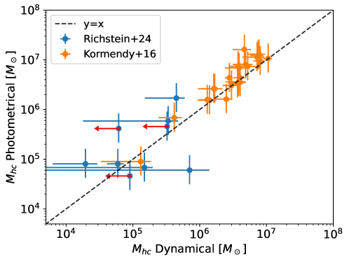
Figure 11: Comparison between the DM halo mass in the core of galaxies computed from the stellar velocity dispersion (horizontal axis) and from photometry alone as described by Eq. (25) (vertical axis). The represented points include UFDs from Richstein+24 Richstein et al. (2024) and dSphs from Kormendy+16 Kormendy and Freeman (2016). The vertical error bars represent the dispersion in $\rho_{c}r_{c}$ (Eq. [3]) whereas the horizontal error bars account for the uncertainties in $\sigma_{\star c}$, as quoted in the original references. The one-to-one line is shown as a dashed black line. The red arrows point out upper limits in the dynamical DM halo masses.

Given the good agreement between the dynamical DM mass and the photometric DM mass represented in Fig. 11, Eq. (25) seems to be a new valuable tool for estimating the DM halo mass from photometry alone. Photometry is much cheaper observationally than the spectroscopy required to determine the dynamical mass. The validity of Eq. (25) implies the validity of Eq. (26), which also provides a new empirical way of estimating the baryon fraction in galaxies only from stellar photometry. Moreover, it tells us that the surface density of stars is a proxy for the baryon fraction in the inner parts of a galaxy.

The above estimate can be extended to the mass of the whole DM halo using a model to represent the DM halo beyond the core (e.g., the piecewise profile in Eq. [7] and Fig. 6). Thus, $M_{hc}$ can be used to estimate $M_{h}$. To have a first idea of the ratio between them, assume that the stelar core radius is not very different from the matching radius $r_{m}$ that separates the inner and outer parts of the piecewise profile (Fig. 6), which is a quite common assumption in the literature (e.g., Lin and Loeb, 2016; Outmezguine et al., 2023). Then, the ratio of masses turns out to be

$$M_{h}/M_{hc}\simeq\frac{\ln(1+r_{\star c}/r_{s})-(r_{\star c}/r_{s})/(1+r_{\star c}/r_{s})}{\ln(1+c)-c/(1+c)},$$ (29)

which varies from a few to a factor of ten when the concentration varies as predicted, from $c\sim 5$ in high mass halos to $c\sim 20$ in low mass halos (Fig. 8, the blue lines).

5.3 Constant DM dynamical pressure

The dynamical pressure in a fluid scales like the density times the square of the characteristic velocity. Thus, for the DM in the core, the effective DM dynamical pressure is

$$P_{c}\propto\rho_{c}\sigma_{c}^{2},$$ (30)

with $\sigma_{c}$ the velocity dispersion of the DM particles in the core. Assuming the DM cores to be virialized (i.e., assuming that Eqs. [27] and [28] hold for the DM particles too), then

$$P_{c}\propto(\rho_{c}\,r_{c})^{2}\simeq{\rm constant},$$ (31)

so that Eq. (1) implies that the dynamical pressure to be exerted by the DM particles if they could collide would be the same in all halos, independently of their total mass or size. But collisionless CDM particles do not collide, and Eq. (31) has to be interpreted as a property that emerges from the existence of the $c$–$M_{h}$ relation.

6 Conclusions

We reviewed the observational evidence for $\rho_{c}r_{c}\simeq$ constant (Eq. [1]; Sect. 2) and then put forward a simple version of the commonly accepted interpretation behind it (Sect. 3). Equation (1) requires the existence of a core in the DM distribution. Halos formed in DM-only CDM cosmological numerical simulations do not have inner cores but cusps (Eq. [4]), however, if any physical process redistributes the DM particles of the expected CDM halos then Eq. (1) is satisfied automatically. It emerges from the relation between concentration and DM halo mass expected in $\Lambda$CDM cosmological simulations. This relation is set by the time of halo formation, so that low mass halos formed earlier and now they present larger concentration (Sect. 5.1). The conventional explanation to understand how the original cuspy CDM halos become cored halos is stellar feedback. This term encapsulates all the baryon driven processes that shuffles gas and mass around (e.g., supernova explosions or stellar winds), modifying the overall potential, including the distribution of DM particles in the center of galaxies Governato et al. (2010); Pontzen and Governato (2014). However, this transformation is not specific to stellar feedback, keeping in mind that any physical process that thermalizes a self gravitating structure tends to form cores Plastino and Plastino (1993); Sánchez Almeida et al. (2020). Thus, any other sensible physical process that redistributes matter without altering the original mass of the CDM halos is able to account for Eq. (1). In other words, the property of $\rho_{c}r_{c}$ to be approximately constant is not specific to CDM but, rather, it is also expected in many alternative DM theories forming cores (e.g., Lin and Loeb, 2016; Kaplinghat et al., 2016; Correa et al., 2022). Theories that only redistribute mass to produce cores have the advantage of leaving the large scale structure of the Universe unchanged, thus being in agreement with the standard $\Lambda$CDM.

The mathematical development in Sect. 3 parallels others existing in the literature, except that the core is modeled with a different expression (e.g., Lin and Loeb, 2016; Kaneda et al., 2024). Here we provide a full account of the derivation of the main equations for the sake of comprehensiveness, which help us to make the qualitative comparison with observations in Sect. 4. However, we could have started off by assuming the relevant Eqs. (12) and (13) and proceed from here. This loose dependence of the results on the actual shape of the core is consistent with the fact that other alternative forms of the piecewise profile with core that we tried (top hat profiles) render qualitatively similar results.

The agreement between the simple theory and observations is notable, keeping in mind that there is no fitting or fine tuning in matching lines and points in Fig. 10. Even more, the theory predicts a moderate increase of $\rho_{c}r_{c}$ with $M_{h}$ similar to the one hinted at by the observations. However, the best fitting $c$–$M_{h}$ relations correspond to large cores (the green dashed line represents $r_{m}/r_{s}=1.8$) or $z\not=0$ (the solid orange and green lines in Fig. 10 correspond to $z=1$). The latter is a result that we do not understand; even if the transformation of cusps to cores requires time and starts at high redshift, the accretion of DM in the outskirts of the halos should continue all the way to the present, a process leading to the $c$–$M_{h}$ relation at $z=0$. As we discuss in Sect. 5.1, the $c$–$M_{h}$ depends on the cosmological parameters $\sigma_{8}$ and $\Omega_{m}$ since they set the assembly time of the DM halos. Varying them may improve the agreement when employing the theoretical $c$–$M_{h}$ relations at $z=0$, but we have not pursued this idea further.

As a byproduct of the effort to compile $\rho_{c}r_{c}$ values, we show that the fact that the product is constant can be used to estimate the mass in the DM halo of a galaxy from the distribution of stars alone. This possibility can be very useful for low stellar mass galaxies where the determination of their DM content using traditional kinematical measurements is technically difficult, whereas their photometry is doable. The same argument allows one to estimate the baryon fraction in the core of these systems. Dwarf galaxies also tend to show a core in the stellar distribution (e.g., Carlsten et al., 2021; Montes et al., 2024), with the radii of the stellar and DM cores expected to scale with each other Sánchez Almeida et al. (2024a, b). This idea plus Eq. (3) allow us to propose specific relations between the observed stellar core radius and the DM core mass (Eq. [25]) and between the observed stellar mass surface density and the baryon fraction in the core (Eq. [26]). The latter tells us that the surface density of stars is a proxy for the baryon fraction in the inner parts of a galaxy. The proposed calibrations are in good agreement with DM masses estimated from dynamical measurements in low mass galaxies (Fig. 11). Note that the numerical coefficients of the proposed scaling laws depend on the definition of core radius, for which we adopted Eq. (2). Other definitions can be trivially recalibrated.

This research has been partly funded through grant PID2022-136598NB-C31 (ESTALLIDOS8) by MCIN/AEI/10.13039/501100011033 and by “ERDF A way of making Europe”. It was also supported by the European Union through the grant ”UNDARK” of the widening participation and spreading excellence programme (project number 101159929).

All the data used in this paper are publicly available in the cited references.

Appendix A Bibliography on the $\rho_{c}r_{c}$ versus $M_{h}$ relation

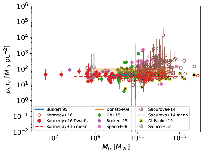
Figure 12: Figure identical to Fig. 1 except that the range of the ordinates ($\rho_{c}r_{c}$) has been expanded to show the same eight orders of magnitude variation as the DM halo mass range ($M_{h}$). For the rest of details, see Fig. 1.

Table 1: References used to constraint $\rho_{c}r_{c}$.

Reference	$\rho_{c}r_{c}$ $[M_{\odot}\,{\rm pc}^{-2}]$ 1	$\log M_{h}$ $[M_{\odot}]$ 2	Comment 3
Burkert (1995) Burkert (1995)	$41.5\pm 5.9$	$10.2\pm 0.4$	Corrected $r_{c}$ & $M_{h}$
Donato et al. (2009) Donato et al. (2009)	$76^{+43}_{-16}$	$8.5$ – $12.5$	Corrected $r_{c}$; $M_{h}$ from $M_{B}$
Burkert (2015) Burkert (2015)	$64^{+56}_{-34}$	$9.0\pm 0.6$	Corrected $r_{c}$
Oh et al. (2015) Oh et al. (2015)	$67\pm 65$	$10.4\pm 0.4$	sigma-clipping in noise
Kormendy and Freeman (2016) Kormendy and Freeman (2016)	$39\pm 17$	$11.5\pm 0.6$	Massive galaxies. Corrected $r_{c}$
Kormendy and Freeman (2016) Kormendy and Freeman (2016)	$40\pm 17$	$9.1\pm 0.8$	Dwarfs. Corrected $r_{c}$
Kormendy and Freeman (2016) Spano et al. (2008)	$230\pm 300$	$11.5\pm 0.5$	Corrected $r_{c}$
Saburova and Del Popolo (2014) Saburova and Del Popolo (2014)	$59\pm 36$	$8.6$ – $11$	Only low mass. Corrected $r_{c}$.
Salucci et al. (2012) Salucci et al. 2012	$71\pm 40$	$9.0\pm 0.4$	dSph only. Corrected $r_{c}$
Di Paolo et al. (2019) Di Paolo et al. 2019	$41\pm 21$	$9.2$ – $13.7$	Corrected $r_{c}$, using their $M_{h}$.

¹ Mean and standard deviation of the values mentioned in the reference.

² Mean and standard deviation or range of values.

³ Further details given in Appendix A.

This appendix details the use of the bibliography leading to Figs. 12, 1, 3, 4, 5, and 10. Since the estimate of the parameters is cumbersome, we discuss the main issues and assumptions in this Appendix and in Table 1. The various references are identified in the figures through the corresponding insets.

• Burkert (1995) Burkert (1995) explicitly gives a relation between central density and core radius and between halo mass and core radius. Pieced together, they provide the relation represented in Fig. 1 with $M_{h}$ within the range represented in his Fig. 3. The original relations have to be corrected to our core radius definition (Eq. [2]) and to the total halo mass (his Eq. [4]).

• Donato et al. (2009) Donato et al. (2009). The value with error bars is directly given in the paper. They conclude that the product $\rho_{c}r_{c}$ is constant for absolute magnitudes $M_{B}$ from -7 to -22. In order to transform these $B$ magnitudes into halo masses, (1) we use a stellar mass to light ratio $M_{\star}/L_{\star}$ of one (in solar units) and then use $M_{\star}$ to estimate $M_{h}$ using the halo to stellar mass ratio at redshift zero from Behroozi et al. (2013). They use the same definition of core radius as Burkert (1995), and so has to be corrected to ours in Eq. (2).

• Burkert (2015) Burkert (2015). We take $\rho_{c}$ and $r_{c}$ from Burkert (2015), and the corresponding $M_{\star}$ from McConnachie (2012). Then $M_{h}$ was estimated using the halo to stellar mass ratio from Behroozi et al. (2013). The conversion between the core radius used in the original work and Eq. (2) was carried out based on Fig. 1 of Burkert (2015).

• Oh et al. (2015) Oh et al. (2015) do not determine the product $\rho_{c}r_{c}$, but they provide $\rho_{c}$ and $r_{c}$ separately. They also provide the absolute $V$ magnitude $M_{V}$ which, assuming a mass to light ratio of one, allows us to estimate $M_{h}$ using the DM halo to stellar mass ratio from Behroozi et al. (2013). The $r_{c}$ used in this reference happens to agree with Eq. (2) and so we do not change it. The averages in Table 1 were computed after removing the $\rho_{c}r_{c}$ values with larger error (see Fig. 1).

• Kormendy and Freeman (2016) Kormendy and Freeman (2016) is the reference with the largest number of galaxies. It gives clear relations between $\rho_{c}$ and $r_{c}$, and $M_{B}$. The galaxies are separated in low and high masses. As for many of the above references, $M_{h}$ is obtained from their $M_{B}$ assuming a stellar mass to light ratio of one, and using the scaling between stellar and halo mass in Behroozi et al. (2013). For the core radius, the authors directly provide the scaling between their core radius and Eq. (2).

• Spano et al. (2008) Spano et al. (2008) also find approximately constant $\rho_{c}r_{c}$. The galaxies are fairly massive (see Table 1). No error bars are given. We transform their $r_{s}$ into ours.

• Saburova and Del Popolo (2014) Saburova and Del Popolo (2014) compile a large list of objects from various sources. The authors compute and provide the product $\rho_{c}r_{c}$. We infer $M_{h}$ from $M_{B}$ as explained above. The points without error bars in Fig. 1 are not points with zero error but points without an estimate of the error. They claim a variation with luminosity so that the more luminous (and so more massive) galaxies have larger $\rho_{s}r_{s}$ (see Fig. 1). The low mass value is consistent with other estimates. They use a Burkert DM halo to define the radius, which we transform to our definition in Eq. (2).

• Salucci et al. (2012) Salucci et al. (2012). We consider only the data for the dwarf spheroidal galaxies (dSph).

• Di Paolo et al. (2019) Di Paolo et al. (2019). These are low surface brightness galaxies, but seem to behave as the rest. Galaxies are stacked in halo mass bins. We take the halo mass from them and then correct $r_{c}$ to accommodate their definition (Burkert profile) into our definition (Eq. [2]).

Appendix B The theoretical value of $\rho_{c}r_{c}$ when $r_{m}=r_{s}$

In the case when the matching radius of the piecewise profile is equal to the characteristic radius of the corresponding NFW profile ($r_{m}/r_{s}=1$ in Fig. 6) then several numerical coincidences happen and $\rho_{c}r_{c}$ and $\rho_{s}r_{s}$ are almost equal,

$$\frac{\rho_{c}r_{c}}{\rho_{s}r_{s}}=\frac{8[3(\ln 2-1/2)]^{5/2}\,[2^{2/5}-1]^{1/2}}{[12(\ln 2-1/2)-1]^{1/2}}\simeq 1.0068\dots.$$ (32)

It follows from Eqs. (6), (12), and (13) when $r_{m}=r_{s}$.

References

References

- Persic et al. (1996) Persic, M.; Salucci, P.; Stel, F. The universal rotation curve of spiral galaxies — I. The dark matter connection. MNRAS 1996, 281, 27–47, [arXiv:astro-ph/astro-ph/9506004]. https://doi.org/10.1093/mnras/278.1.27.
- Oh et al. (2015) Oh, S.H.; Hunter, D.A.; Brinks, E.; Elmegreen, B.G.; Schruba, A.; Walter, F.; Rupen, M.P.; Young, L.M.; Simpson, C.E.; Johnson, M.C.; et al. High-resolution Mass Models of Dwarf Galaxies from LITTLE THINGS. AJ 2015, 149, 180, [arXiv:astro-ph.GA/1502.01281]. https://doi.org/10.1088/0004-6256/149/6/180.
- Salucci (2019) Salucci, P. The distribution of dark matter in galaxies. A&A Rev. 2019, 27, 2, [arXiv:astro-ph.GA/1811.08843]. https://doi.org/10.1007/s00159-018-0113-1.
- Burkert (1995) Burkert, A. The Structure of Dark Matter Halos in Dwarf Galaxies. ApJ 1995, 447, L25–L28, [arXiv:astro-ph/astro-ph/9504041]. https://doi.org/10.1086/309560.
- Salucci and Burkert (2000) Salucci, P.; Burkert, A. Dark Matter Scaling Relations. ApJ 2000, 537, L9–L12, [arXiv:astro-ph/astro-ph/0004397]. https://doi.org/10.1086/312747.
- Spano et al. (2008) Spano, M.; Marcelin, M.; Amram, P.; Carignan, C.; Epinat, B.; Hernandez, O. GHASP: an H kinematic survey of spiral and irregular galaxies - V. Dark matter distribution in 36 nearby spiral galaxies. MNRAS 2008, 383, 297–316, [arXiv:astro-ph/0710.1345]. https://doi.org/10.1111/j.1365-2966.2007.12545.x.