Foliated Asymptotically Safe Gravity
Lorentzian Signature Fluctuations from the Wick Rotation

Abstract

Asymptotic Safety constitutes a promising mechanism for a consistent and predictive high-energy completion of the gravitational interactions. To date, most results on the interacting renormalization group fixed point underlying the construction are obtained for Euclidean signature spacetimes. In this work, we use the Arnowitt-Deser-Misner (ADM) decomposition of the metric degrees of freedom and investigate the relations between the Euclidean and Lorentzian renormalization group flows resulting from the analytic continuation of the lapse function. We discuss the general conditions which guarantee the equivalence of the beta functions. These insights are illustrated based on the flow of the graviton two-point function within the Einstein-Hilbert truncation, demonstrating agreement of the Euclidean and Lorentzian settings. Hence the UV- and IR-completions identified in the Euclidean case are robust when changing spacetime signature. We take this as an important indicator that the Euclidean asymptotic safety mechanism carries over to Lorentzian signature spacetimes.

I Introduction

The construction of a ultraviolet (UV)-complete quantum field theory of gravity is still an open question in modern theoretical physics. One candidate for such a theory is the gravitational asymptotic safety program [1, 2] also reviewed in [3, 4, 5, 6, 7, 8, 9, 10, 11]. Starting from Weinberg’s initial conjecture [12], the Wetterich equation [13, 14] adapted to gravity [15], has provided substantial evidence that the gravitational renormalization group (RG) flow indeed possesses an interacting fixed point which could render gravity asymptotically safe [16, 17, 18, 19, 20, 21, 22, 23, 24, 25]. This fixed point, called the Reuter fixed point, also extends to a variety of gravity-matter systems [26, 27, 28, 29, 30, 31, 32, 33, 34, 35, 36, 37, 38, 39, 40, 41, 42, 43, 44, 45], making the program attractive for a wide range of phenomenological applications including particle physics [46], black hole physics [47, 48], and cosmological applications [49, 50]. Links to other approaches to quantum gravity, including Causal Dynamical Triangulations (CDT) [51, 52], canonical quantization [53, 54], and swampland conjectures [55, 56, 57, 58] have recently been explored as well.

Most investigations related to Asymptotic Safety are carried out in a Euclidean background spacetime. In order to arrive at a more realistic description of nature spacetime should come with Lorentzian signature though. Drawing inspiration from quantum field theory in a curved spacetime [59], this transition introduces a series of new elements

1. As compared to the Euclidean setting, the Lorentzian setup requires a new geometric structure - essentially a preferred direction - which is associated with time. This affects, e.g., the space of fluctuations in the metric field [60].

2. In contrast to the Euclidean case, propagators and the choice of vacuum are no longer unique as soon as the background spacetime is sufficiently generic.

3. In a quantum field theory defined on a flat, non-dynamical Euclidean background, the analytic continuation from a Euclidean to Lorentzian spacetime is implemented by the Wick rotation of the time-coordinate, $\tau^{\rm E}\rightarrow i\tau^{\rm L}$. When it comes to gravity on a general curved spacetime, this prescription could lead to complex and unphysical metrics if $g_{\mu\nu}$ depends on time explicitly [61].

These points posit a clear mandate for investigating the working of the asymptotic safety mechanism also for Lorentzian signature spacetime, leading to the Lorentzian asymptotic safety program.

Starting from [62], the impact of spacetime signature has been explored from various angles. Formally, one can derive the Wetterich equation from a path integral formulated in Lorentzian signature. Borrowing tools developed in the context of algebraic quantum field theory allows to formulate this equation in a background-independent way [63, 64]. This strategy highlights the state-dependence of the Lorentzian construction [65, 66]. On the technical side, these developments have been complemented by developing heat-kernel methods for Lorentzian metrics on real manifolds [67]. Along a different path, the fluctuation approach towards solving the Wetterich equation [4] has started from a flat Minkowski background and constructed the spectral function of the graviton on this background [68, 69]. Based on these results, it was argued that the spectral function comprises a massless one-graviton peak and a multi-graviton continuum with an asymptotically safe scaling for large momenta.

The points discussed above lead to the intriguing question whether there is a canonical relation among RG flows obtained in the Euclidean and Lorentzian settings. From a geometrical perspective, the first step towards such a connection is to equip the Euclidean spacetime with a foliation structure. This can either be done by applying the Arnowitt-Deser-Misner (ADM) decomposition to the metric [77, 78] or adding additional geometric objects to the covariant formulation [79]. Asymptotic Safety based on the ADM formalism has already been investigated in a series of works within the background approximation [62, 80, 81] and also in the fluctuation approach focusing on the graviton propagator [82, 83]. A remarkable insight obtained from this line is that the ADM and covariant formulations give rise to very similar results with respect to the existence of interacting renormalization group fixed points and phase diagrams. This is non-trivial, since the two constructions encode the fluctuating degrees of freedom in different fields so that one should expect to deal with different quantum theories on generic grounds [84].

In this work, we complement our understanding of RG flows within the ADM formalisms by studying the Wick rotation from Euclidean to Lorentzian signature spacetimes through the analytic continuation of the lapse function. This avoids the issues related to complex metrics which arises from the analytic continuation of the time coordinate. Furthermore, this prescription may restore the conventional causal Feynman propagator on a Minkowski spacetime [61]. We then identify generic conditions on the propagators and regulators entering in the evaluation of the Wetterich equation which ensure that RG flows in the Euclidean and Lorentzian settings agree.

As a concrete application, we compute the RG flow of the graviton two-point function using the interaction vertices generated by the Einstein-Hilbert action and show that the resulting beta functions obtained in the Lorentzian case are identical to the Euclidean ones. Based on the RG flow, we then identify a suitable interacting fixed point with two relevant directions. This suggests that also Lorentzian quantum gravity can be UV-complete via the asymptotic safety mechanism and constitutes a key step towards relating the Lorentzian asymptotic safety program to existing Euclidean results.

This paper is organized as follows. In Section II, we introduce the ADM decomposition and review the prescription of Wick rotation via complexifying the lapse function. Section III reviews the Wetterich equation and specifies the setup underlying our computation. Our results for the beta functions are given in Section IV and the resulting fixed-point structure and phase diagrams are constructed in Section V. We close with a discussion of our results and outlook in Section VI. The explicit form of the ghost sector entering our computation is given in Appendix A.

II Foliated spacetime
and Wick rotation

We start by reviewing the ADM formalism [77, 78]. We take the spacetime $\mathcal{M}$ as a $d+1$-dimensional manifold admitting a foliation. This spacetime is equipped with coordinates $x^{\mu}$, $\mu=\{0,\cdot\cdot\cdot,d\}$ and a metric $g_{\mu\nu}$. Subsequently, we introduce a scalar function $\tau(x)$. This function foliates $\mathcal{M}$ into a one-parameter family of hypersurfaces $\Sigma_{\tau}$, containing all points with the same value for $\tau$. The existence of such a foliation is a necessary ingredient for transiting from Euclidean to Lorentzian signature spacetimes and constitutes a geometrical structure which is not necessarily present in the Euclidean signature case.

The foliation structure allows us to introduce a new coordinate system, given by the time-coordinate $\tau$ and coordinates $y^{i}$, $i=1,\cdots,d$ providing a coordinate system on $\Sigma_{\tau}$. Assuming Euclidean signature, the line element written in terms of the coordinates $\{\tau,y^{i}\}$ can be given as

$$ds^{2}=N^{2}d\tau^{2}+\sigma_{ij}(N^{i}d\tau+dy^{i})(N^{j}d\tau+dy^{j}).$$ (1)

This decomposition encodes the metric degrees of freedom in the lapse function $N$, the shift vector $N^{i}$, and the metric $\sigma_{ij}$ measuring distances on $\Sigma_{\tau}$. From Eq. (1), the components of the metric tensor are read off as

$$g_{\mu\nu}=\begin{pmatrix}N^{2}+N^{i}N_{i}~~~&N_{j}\\ N_{i}~~~&\sigma_{ij}\\ \end{pmatrix}.$$ (2)

Now, we consider the transition from Euclidean to Lorentzian signature. One way to implement this on a generic, curved spacetime is the analytic continuation of the lapse function [85, 61],

$$N\mapsto\sqrt{\epsilon_{c}}\,N\,.$$ (3)

Here the parameter $\epsilon_{c}$ encodes the contour $c$ taken in the analytic continuation. Substituting this expression into Eq. (2) leads to

$$g^{(\epsilon_{c})}_{\mu\nu}=\begin{pmatrix}\epsilon_{c}N^{2}+N^{i}N_{i}~~~&N_{j}\\ N_{i}~~~&\sigma_{ij}\\ \end{pmatrix}.$$ (4)

One can easily verify that this parametrized metric interpolates between the Euclidean metric for $\epsilon_{c}=+1$ and the Lorentzian metric for $\epsilon_{c}=-1$. As pointed out by [61], if one treats the parameter $\epsilon_{c}$ as a continuous real number, the inverse of the metric (4) will degenerate at $\epsilon_{c}=0$. This suggests to regard $\epsilon_{c}$ as complex with the analytic continuation either along the unit circle in the complex plane or by shifting the path along the real line by a small imaginary part. We will consider the second option, setting

$$\epsilon_{c}=\epsilon_{s}+i\,c\,\epsilon\,,$$ (5)

with $c$ being a real, positive, and field-dependent normalization factor. The real part $\epsilon_{s}$ takes values in the interval $[-1,1]$. The lower and upper boundary corresponds to the Lorentzian and Euclidean signature metric, respectively. The parameter $\epsilon$ ensures that the metric remains regular along the integration contour and is treated as infinitesimal.

It is instructive to illustrate the effect of this analytic continuation at the level of a free scalar field $\phi$ of mass $m$. Setting $N_{i}=0$ for clarity, the ADM-decomposed action is

$$\begin{split}&S[\phi]=\frac{1}{2}\int d\tau d^{d}y\,\sqrt{\epsilon_{s}}N\sqrt{\sigma}\times\\ &\,\,\left(\frac{1}{\epsilon_{s}N^{2}}(\partial_{\tau}\phi)^{2}+\sigma^{ij}(\partial_{i}\phi)(\partial_{j}\phi)+m^{2}\phi^{2}-i\epsilon\phi^{2}\right).\end{split}$$ (6)

Here we expanded to first order in $\epsilon$ and chose the constant $c$ in (5) to ensure standard normalization.

Based on (6), it is straightforward to show that one recovers the causal Feynman propagator on a flat Lorentzian spacetime by inverting the second functional derivative of $S[\phi]$. Setting $N=1$ and $\sigma^{ij}=\delta^{ij}$ and converting to momentum space, denoting the time- and spatial components of the momentum four-vector by $p_{0}$ and $\vec{p}$, respectively, yields

$$\mathcal{G}=\frac{1}{\sqrt{\epsilon_{s}}\left(\epsilon_{s}^{-1}p_{0}^{2}+\vec{p}^{~2}+m^{2}-i\epsilon\right)}\,.$$ (7)

In the Euclidean signature case where $\epsilon_{s}=1$ the denominator is positive definite and the $i\epsilon$-term can be dropped. In the Lorentzian case, Eq. (7) evaluates to

$$\mathcal{G}=\frac{i}{\left(p_{0}^{2}-\vec{p}^{~2}-m^{2}+i\epsilon\right)}\,,$$ (8)

and one recovers the standard $i\epsilon$ prescription of a massive scalar propagator in mostly-plus signature. Hence the prescription (5) recovers the standard Wick-rotation results in a flat spacetime. At the same time, it also applies to the more general case where spacetime is curved, thereby giving a unique relation between Euclidean and Lorentzian signature results. In the remaining part of this paper, we will apply this analytic continuation to the Wetterich equation adapted to the ADM formalism [62, 85], explicitly relating RG flows obtained for Euclidean and Lorentzian signature backgrounds.

III Wetterich equation and
projection schemes

Investigating the asymptotic safety mechanism in the context of gravity requires a method to compute RG flows. The main tool used in these studies is the Wetterich equation [13, 14],

$$k\partial_{k}\Gamma_{k}=\frac{1}{2}\text{STr}\left[\mathcal{G}_{k}\,k\partial_{k}R_{k}\right].$$ (9)

The Wetterich equation encodes the dependence of the effective average action $\Gamma_{k}$ on the coarse-graining scale $k$. Its right-hand side (rhs) contains the scale-dependent propagator $\mathcal{G}_{k}\equiv\left(\Gamma_{k}^{(2)}+R_{k}\right)^{-1}$ where $\Gamma_{k}^{(2)}$ is the second functional derivative of $\Gamma_{k}$ with respect to the quantum field. The propagator has been supplied by a regulator $R_{k}$ which provides a mass term to fluctuations with momentum $p^{2}\lesssim k^{2}$ and vanishes for $p^{2}\gg k^{2}$. The supertrace STr contains the integral over the internal momenta, a sum over the fields, and depends on the signature of spacetime through $\epsilon_{s}$. The interplay of $R_{k}$ in the propagator and the numerator ensures that the trace contribution is finite and peaked on momenta $p^{2}\approx k^{2}$. In this way, the Wetterich equation realizes Wilson’s idea of renormalization, integrating out quantum fluctuations shell-by-shell in momentum space when lowering the coarse-graining scale. For convenience, we will trade $k$ for the dimensionless RG time $t\equiv\text{ln}(k/k_{0})$ where $k_{0}$ is an arbitrary reference scale.

The goal of this work is to use Eq. (9) to investigate the signature-dependence of the gravitational RG flow. For this purpose, we encode the gravitational degrees of freedom in the ADM fields so that the Euclidean and Lorentzian settings can be connected by the analytic continuation of the lapse function (3). We then employ the background field method, splitting the ADM fields into background fields (conventionally distinguished by a bar) and fluctuations (coming with a hat)

$$\begin{split}\sigma_{ij}=\bar{\sigma}_{ij}+\hat{\sigma}_{ij},\,\,\,N_{i}=\bar{N}_{i}+\hat{N}_{i},\,\,\,N=\bar{N}+\hat{N}.\end{split}$$ (10)

For the present study, it is sufficient to adopt a flat background with $\bar{N}=1$, $\bar{N}_{i}=0$, and $\bar{\sigma}_{ij}=\delta_{ij}$. Correlation functions of the fluctuation fields can then be obtained by taking the functional derivatives of $\Gamma_{k}$ with respect to the fluctuations.

In order to reduce the complexity of the computation, we apply the York decomposition [86] to the fluctuation fields

$$\hat{\sigma}_{ij}=h_{ij}+\partial_{i}\frac{1}{\sqrt{\bar{\Delta}}}v_{j}+\partial_{j}\frac{1}{\sqrt{\bar{\Delta}}}v_{i}+\partial_{i}\partial_{j}\frac{1}{\bar{\Delta}}E+\frac{1}{3}\delta_{ij}E+\frac{1}{3}\delta_{ij}\psi\,.$$ (11)

Here the background Laplacian is defined as $\bar{\Delta}\equiv-\delta^{ij}\partial_{i}\partial_{j}$, and the component fields satisfy

$$\partial^{i}h_{ij}=0,\quad\delta^{ij}h_{ij}=0,\quad\partial^{i}v_{i}=0,\quad\psi=\delta^{ij}\hat{\sigma}_{ij}\,.$$ (12)

The decomposition for the shift vector is

$$\hat{N_{i}}=u_{i}+\partial_{i}\frac{1}{\sqrt{\bar{\Delta}}}B,\quad\partial^{i}u_{i}=0\,.$$ (13)

Note that this decomposition is independent of the lapse function $N$. Hence it is unaffected by the analytic continuation (3).

In order to be able to compute the RG flow explicitly we then approximate $\Gamma_{k}$ by the Einstein-Hilbert (EH) action supplemented by gauge-fixing (gf) and ghost terms,

$$\Gamma_{k}\simeq\Gamma^{\text{EH}}_{k}+\Gamma^{\text{gf}}_{k}+\Gamma^{\text{ghost}}.$$ (14)

The Einstein-Hilbert action written in terms of the ADM fields and the substitution (3) is given by

$$\begin{split}\Gamma^{\text{EH}}_{k}=&\frac{1}{16\pi G_{k}}\int d\tau d^{3}y\,\sqrt{\epsilon_{s}}\,N\sqrt{\sigma}\times\,\\ &\left(\epsilon^{-1}_{s}K^{ij}K_{ij}-\epsilon^{-1}_{s}K^{2}-R+2\Lambda_{k}+i\epsilon\right)\,.\end{split}$$ (15)

Here the extrinsic curvature $K_{ij}$ is defined as

$$K_{ij}\equiv\frac{1}{2N}\left(\partial_{\tau}\sigma_{ij}-D_{i}N_{j}-D_{j}N_{i}\right),$$ (16)

with $D_{i}$ being the covariant derivative defined with respect to the spatial metric $\sigma_{ij}$, $R$ is the Ricci scalar constructed from $\sigma_{ij}$, and the $i\epsilon$ acts as a reminder that for Lorentzian signature poles in the propagator are shifted away from the axis of integration. The approximation (15) tracks the flow of two couplings, Newton’s coupling $G_{k}$ and the cosmological constant $\Lambda_{k}$ which have been promoted to functions of the coarse-graining scale $k$.

Finally, we need to specify gauge-fixing and ghost terms. As pointed out by [80, 87], the two-point vertices generated by the Einstein-Hilbert action in the ADM formalism are non-relativistic in general. This can be fixed by adopting harmonic gauge [81]. Including the terms quadratic in the fluctuations then gives the following gauge-fixing action,

$$\Gamma^{\text{gf}}_{k}=\frac{1}{32\pi G_{k}}\int\mathrm{d}\tau\mathrm{d}^{3}y\sqrt{\epsilon_{s}}\left(\epsilon_{s}F^{2}+\delta^{ij}F_{i}F_{j}\right)\,,$$ (17)

with the gauge-fixing conditions,

$$\begin{split}F&=\frac{1}{{\epsilon_{s}}}\partial_{\tau}\hat{N}+\frac{1}{{\epsilon_{s}}}\partial^{i}\hat{N}_{i}-\frac{1}{{\epsilon_{s}}}\frac{1}{2}\partial_{\tau}\psi\,,\\ F_{i}&=\frac{1}{{\epsilon_{s}}}\partial_{\tau}\hat{N}_{i}-\partial_{i}\hat{N}-\frac{1}{2}\partial_{i}\psi+\partial^{j}\hat{\sigma}_{ij}.\end{split}$$ (18)

The ghost term resulting from this choice is obtained by the standard Faddeev-Popov procedure and is given in Appendix A.

According to [88, 89], the transverse-traceless (TT)-mode $h_{ij}$ encodes the tensor fluctuations in a gauge-invariant way. It is the two-point function of this field which is related to observations. Therefore, we will read off the flow equations for $G_{k}$ and $\Lambda_{k}$ from the propagator of $h_{ij}$. Conceptually, this corresponds to a fluctuation field computation along the lines described in [90, 4]. In general, the scale dependence of an $n$-point vertex is obtained from (9) by taking derivatives with respect to the corresponding fluctuation fields, collectively denoted by $\hat{\chi}$. Schematically,

$$\partial_{t}\Gamma^{(n)}_{k}=\frac{1}{2}\text{STr}\left[\frac{\delta^{n}}{\delta\hat{\chi}^{n}}\,\mathcal{G}_{k}\,\partial_{t}R_{k}\,\right].$$ (19)

For the two-point correlation function of $h_{ij}$ this general expression evaluates to

$$\begin{split}\partial_{t}\Gamma^{(hh)}_{k}=&\;{\rm STr}\Big{[}\mathcal{G}_{k}\;\Gamma_{k}^{(3)}\;\mathcal{G}_{k}\Gamma_{k}^{(3)}\;\mathcal{G}_{k}\;\partial_{t}\mathcal{R}_{k}\Big{]}\\ &-\frac{1}{2}{\rm STr}\left[\mathcal{G}_{k}\;\Gamma_{k}^{(4)}\;\mathcal{G}_{k}\;\partial_{t}\mathcal{R}_{k}\right]\,.\end{split}$$ (20)

Here $\Gamma_{k}^{(3)}$ and $\Gamma_{k}^{(4)}$ denote the three- and four-point vertices obtained from $\Gamma_{k}$. Here, it is tacitly understood that the terms on the rhs come with two external graviton legs and momentum $p^{2}$. In order to close the system, we then generate the interaction vertices from (14). This completes our computational framework.

The first step in evaluating (20) is the construction of the required $n$-point vertices. This can be easily done using computer algebra software [91, 92]. The two-point functions resulting from this procedure are collected in Table 1.

fields	components of $\Gamma_{k}^{(2)}$
$h_{ij}h^{kl}$	$\frac{1}{32\pi G_{k}}\sqrt{\epsilon_{s}}\left(({\epsilon_{s}^{-1}}p_{0}^{2}+\vec{p}^{\,2})-2\Lambda_{k}\right)\,{\Pi_{h}}^{ij}_{~~kl}$
$v_{i}v^{j}$	$\frac{1}{16\pi G_{k}}\sqrt{\epsilon_{s}}\left(({\epsilon_{s}^{-1}}p_{0}^{2}+\vec{p}^{\,2})-2\Lambda_{k}\right){\Pi_{u}}{}^{i}{}_{j}$
$EE$	$\frac{1}{48\pi G_{k}}\sqrt{\epsilon_{s}}\left(({\epsilon_{s}^{-1}}p_{0}^{2}+\vec{p}^{\,2})-2\Lambda_{k}\right)$
$\Psi\Psi$	$-\frac{1}{192\pi G_{k}}\sqrt{\epsilon_{s}}\left({\epsilon_{s}^{-1}}p_{0}^{2}+\vec{p}^{\,2}-2\Lambda_{k}\right)$
$\hat{N}\hat{N}$	$\frac{1}{16\pi G_{k}}\sqrt{\epsilon_{s}}({\epsilon_{s}^{-1}}p_{0}^{2}+\vec{p}^{\,2})$
$\Psi\hat{N}$	$-\frac{1}{16\pi G_{k}}\sqrt{\epsilon_{s}}\left({\epsilon_{s}^{-1}}p_{0}^{2}+\vec{p}^{\,2}-2\Lambda_{k}\right)$
$u^{i}u_{j}$	$\frac{1}{16\pi G_{k}}{\epsilon_{s}^{-1/2}}({\epsilon_{s}^{-1}}p_{0}^{2}+\vec{p}^{\,2}){\Pi_{u}}{}^{i}{}_{j}$
$BB$	$\frac{1}{16\pi G_{k}}{\epsilon_{s}^{-1/2}}\left({\epsilon_{s}^{-1}}p_{0}^{2}+\vec{p}^{\,2}\right)$
$\bar{c}c$	$-\,\sqrt{\epsilon_{s}}(p^{2}_{0}+\epsilon_{s}\vec{p}^{\,2})$
$\bar{b}^{i}b_{i}$	$-\,\sqrt{\epsilon_{s}}({\epsilon_{s}^{-1}}p^{2}_{0}+\vec{p}^{\,2})\,\Pi_{u}{}_{j}{}^{i}$

Table 1: Matrix elements of the two-point functions $\Gamma^{(2)}_{k}$ including the analytic continuation of the lapse function (5). Here $\Pi$ are the standard tensor structures associated with the internal indices of the fluctuation fields [1] and the $i\epsilon$ terms relevant in the Lorentzian setting are suppressed for the sake of readability.

Owed to the gauge choice (17), all two-point functions (and propagators) come with a relativistic dispersion relation. Moreover, the cosmological constant serves as a mass term in some of the two-point functions. This also includes the correlation function for $h$.

Next, we need to specify the regulator $R_{k}$. In the Euclidean setting, the quantity separating the fluctuations into high- and low-momentum modes is taken as the magnitude of the momentum four-vector $p^{2}=p_{0}^{2}+\vec{p}^{2}$ which is positive definite. This leads to an intuitive ordering in which fluctuations with large four-momentum are integrated out first. The Lorentzian signature analogue $p^{2}=-p_{0}^{2}+\vec{p}^{2}$ is no longer positive definite though, making the discrimination of high- and low-momentum modes more subtle. In addition, the regulator may alter the analytic properties of $\mathcal{G}_{k}$, by inducing new poles in the complex momentum plane. Such an improper regularization procedure may then spoil the connection between the evaluation of the trace in (9) in Euclidean and Lorentzian signature backgrounds, also see [93] for a related discussion.

In order to ameliorate these subtleties, we opt for a regulator which discriminates high- and low-momentum modes according to their spatial momentum $\vec{p}^{\,2}$. Based on this choice, we follow [62, 66] and implement the Type I regularization by replacing

$$\vec{p}^{\,2}\mapsto\vec{p}^{\,2}+R_{k}(\vec{p}^{\,2}).$$ (21)

The regulator function $R_{k}(\vec{p}^{\,2})$ is taken of Litim-type $R_{k}(\vec{p}^{\,2})=(k^{2}-\vec{p}^{\,2})\Theta(k^{2}-\vec{p}^{\,2})$, with $\Theta$ being the Heaviside step function [94, 95]. This is sufficient to render the momentum integrals in the STr finite, thus meeting the finiteness criterion (finiteness). It also guarantees that there are no additional poles appearing in the complex $p_{0}$-plane as this choice also acts as a mass term in the Lorentzian signature setting (analyticity). These features come at the expense that the regulator breaks Lorentz invariance explicitly though. Thus, the structural features of the choice (21) are summarized as follows

$$\begin{array}[]{c|c|c}&\quad{\rm yes}&\quad{\rm no}\\ \hline\cr\Big{.}{\rm finiteness}&{\bf X}&\\ \Big{.}{\rm analyticity}&{\bf X}&\\ \Big{.}\quad{\rm Lorentz\;symmetry}&&{\bf X}\\ \hline\cr\end{array}$$ (22)

Currently, there is no known regularization function which meets all three criteria simultaneously. It is the trade between analyticity and Lorentz symmetry which then distinguishes the present analysis from the previous work [82] and also the regularization procedures employed in the fluctuation computations in the covariant setting [4].

Finally, we specify our projection scheme. Our goal is to determine the flow of the two-point function $\Gamma_{k}^{(hh)}$ given in the first line of Table 1. Hence we project onto

$$\Gamma^{(hh)}_{k}=\frac{1}{32\pi G_{k}}\sqrt{\epsilon_{s}}\left((\epsilon^{-1}_{s}p^{2}_{0}+\vec{p}^{\,2})-2\Lambda_{k}\right){\Pi_{h}}^{ij}_{kl}\,.$$ (23)

In this way $-2\Lambda_{k}\equiv\mu_{k}^{2}$ acquires the interpretation as the graviton mass while $G_{k}$ has the status of a wave-function renormalization. Substituting $\Gamma_{k}^{(hh)}$ into the left-hand side of the Wetterich equation yields

$$\partial_{t}\Gamma^{(hh)}_{k}=\frac{1}{32\pi}\sqrt{\epsilon_{s}}\left((\epsilon^{-1}_{s}p^{2}_{0}+\vec{p}^{\,2})\partial_{t}\frac{1}{G_{k}}-2\partial_{t}\frac{\Lambda_{k}}{G_{k}}\right){\Pi_{h}}^{ij}_{kl},$$ (24)

where $\Pi_{h}$ is the projection tensor which projects a rank two symmetric tensor onto its TT component. The beta function for $\Lambda_{k}$ can then be read off from the momentum-independent part of the two-point function. In order to obtain the beta function of $G_{k}$, one can either project onto the $p^{2}_{0}$ or $\vec{p}^{\,2}$ component of (24). We refer to these projections as the $p_{0}$- and $\vec{p}$-projection, respectively. The comparison between two projections gives an estimate for the size of Lorentz symmetry breaking effects.

IV Beta functions

The computation of the beta functions encoding the $k$-dependence of the two-point function (20) can be organized along the lines taken in [82]. When evaluating the momentum integrals on the rhs, the real part of the parameter $\epsilon_{s}$ is fixed to $1$ and $-1$, corresponding to Euclidean and Lorentzian signature, respectively. In addition, we retain the $i\epsilon$-prescription for the momentum integration in the Lorentzian setting. The loop integrals are then evaluated in each case. As the main result of this work, this computation shows that the Euclidean and Lorentzian RG flows are identical. This feature follows from the analyticity property of the regulator (21) which leads to identical values for the loop integral under the transformation (3). As a consequence, there is no need to distinguish between the Euclidean and Lorentzian signature RG flows in the sequel and all our results apply to both cases.

The $k$-dependence of the dimensionless couplings $g_{k}\equiv G_{k}k^{2}$ and $\lambda_{k}\equiv\Lambda_{k}/k^{2}$ is encoded in the beta functions

$$\partial_{t}\lambda_{k}=\beta_{\lambda}(g_{k},\lambda_{k})\,,\qquad\partial_{t}g_{k}=\beta_{g}(g_{k},\lambda_{k})\,.$$ (25)

The explicit computation yields

$$\begin{split}\beta_{g}=&\,\left(2+\eta_{N}\right)g\,,\\ \beta_{\lambda}=&\,(\eta_{N}-2)\lambda+\frac{g}{4725\,\lambda^{2}\,\pi}\\ &\bigg{(}w^{1}_{\lambda}+\eta_{N}\tilde{w}^{1}_{\lambda}+\frac{w^{2}_{\lambda}+\eta_{N}\tilde{w}^{2}_{\lambda}}{(1-2\lambda)^{5/2}}+\frac{w^{3}_{\lambda}+\eta_{N}\tilde{w}^{3}_{\lambda}}{(1-\frac{3}{2}\lambda)^{5/2}}\bigg{)}\,.\end{split}$$ (26)

The $w_{\lambda}^{i}$ and $\tilde{w}_{\lambda}^{i}$ are polynomials in $\lambda$ and listed in the first block of Table 2.

$\bigg{.}w^{1}_{\lambda}$	$15525\lambda^{2}+8652\lambda-2324$
$\bigg{.}\tilde{w}^{1}_{\lambda}$	$135\lambda^{2}-1236\lambda+332$
$\bigg{.}w^{2}_{\lambda}$	$-6\left(300545\lambda^{4}-527933\lambda^{3}+383491\lambda^{2}-127872\lambda+16546\right)$
$\bigg{.}\tilde{w}^{2}_{\lambda}$	$2\left(180327\lambda^{4}-296517\lambda^{3}+198772\lambda^{2}-60696\lambda+7178\right)$
$\bigg{.}w^{3}_{\lambda}$	$2\left(375795\lambda^{4}-912849\lambda^{3}+822489\lambda^{2}-330252\lambda+50800\right)$
$\bigg{.}\tilde{w}^{3}_{\lambda}$	$-150318\lambda^{4}+344733\lambda^{3}-288828\lambda^{2}+105928\lambda-14688$
$\bigg{.}w^{4}_{\lambda}$	$-135\lambda^{4}+34776\lambda^{3}+132216\lambda^{2}-433664\lambda+71120$
$\bigg{.}w^{5}_{\lambda}$	$164498565\lambda^{6}-500454234\lambda^{5}+641684601\lambda^{4}-443566412\lambda^{3}+174167272\lambda^{2}-36783720\lambda+3259992$
$\bigg{.}w^{6}_{\lambda}$	$-4329575145\lambda^{6}+15697970316\lambda^{5}-23841861804\lambda^{4}+19445619456\lambda^{3}-8995973376\lambda^{2}+2240897024\lambda-235003904$
$\bigg{.}\tilde{w}^{4}_{\lambda}$	$-\left(2025\lambda^{4}+4968\lambda^{3}+18888\lambda^{2}-61952\lambda+10160\right)$
$\bigg{.}\tilde{w}^{5}_{\lambda}$	$-98699139\lambda^{6}+285744222\lambda^{5}-347335841\lambda^{4}+227082460\lambda^{3}-84266056\lambda^{2}+16831752\lambda-1413816$
$\bigg{.}\tilde{w}^{6}_{\lambda}$	$865915029\lambda^{6}-3011887260\lambda^{5}+4362687516\lambda^{4}-3374371584\lambda^{3}+1473101568\lambda^{2}-345042944\lambda+33972224$
$\bigg{.}w^{7}_{\lambda}$	$-3699\lambda^{3}+9360\lambda^{2}+8532\lambda-30016$
$\bigg{.}w^{8}_{\lambda}$	$-1272480\lambda^{6}+20671730\lambda^{5}-46807002\lambda^{4}+45990965\lambda^{3}-23327508\lambda^{2}+6039068\lambda-634560$
$\bigg{.}w^{9}_{\lambda}$	$31978800\lambda^{6}-559973655\lambda^{5}+1544967540\lambda^{4}-1848096396\lambda^{3}+1141774848\lambda^{2}-361502976\lambda+46888960$
$\bigg{.}\tilde{w}^{7}_{\lambda}$ $(\lambda)$	$-4\left(135\lambda^{2}+780\lambda-497\right)$
$\bigg{.}\tilde{w}^{8}_{\lambda}$	$-212080\lambda^{4}+113424\lambda^{3}+119699\lambda^{2}-103028\lambda+20244$
$\bigg{.}\tilde{w}^{9}_{\lambda}$	$-394800\lambda^{3}+129321\lambda^{2}+299328\lambda-125440$

Table 2: Polynomials $w^{i}_{\lambda}$ and $\tilde{w}^{i}_{\lambda}$ introduced in the beta functions (26) (top block), the anomalous dimension (27) for the $p_{0}$-projection (middle block), and $\vec{p}$-projection (lower block).

The anomalous dimension can be cast into the form

$$\eta_{N}=\frac{g\,B_{1}(\lambda)}{1-g\,B_{2}(\lambda)}\,.$$ (27)

The functions $B_{1}(\lambda)$ and $B_{2}(\lambda)$ can be evaluated by projecting onto either the set $\{p^{2}_{0}~\Pi_{h},\Pi_{h}\}$ ($p_{0}$-projection) or $\{{\vec{p}}^{~2}\Pi_{h},\Pi_{h}\}$ ($\vec{p}$-projection). In a Lorentz-covariant setting, these projections would give identical results. Owed to the Lorentz-symmetry breaking contributions, the two projections lead to different results. For the $p_{0}$-projection we find

$$\begin{split}B_{1}^{p_{0}}=&\frac{1}{1575\pi\lambda^{4}}\Bigg{(}\frac{w^{4}_{\lambda}}{18}+\frac{w^{5}_{\lambda}}{(1-2\lambda)^{7/2}}+\frac{w^{6}_{\lambda}}{72(1-\frac{3}{2}\lambda)^{7/2}}\Bigg{)}\,,\\ B_{2}^{p_{0}}=&\frac{1}{4725\pi\lambda^{4}}\Bigg{(}\frac{\tilde{w}^{4}_{\lambda}}{6}+\frac{\tilde{w}^{5}_{\lambda}}{(1-2\lambda)^{7/2}}+\frac{\tilde{w}^{6}_{\lambda}}{24(1-\frac{3}{2}\lambda)^{7/2}}\Bigg{)}\,,\end{split}$$ (28)

while the $\vec{p}$-projection leads to

$$\begin{split}B_{1}^{\vec{p}}=&\frac{1}{315\pi\lambda^{3}}\Bigg{(}\frac{w^{7}_{\lambda}}{9}+\frac{w^{8}_{\lambda}}{5(1-2\lambda)^{7/2}}+\frac{w^{9}_{\lambda}}{360(1-\frac{3}{2}\lambda)^{7/2}}\Bigg{)},\\ B_{2}^{\vec{p}}=&\frac{1}{1575\pi\lambda^{2}}\Bigg{(}\frac{\tilde{w}^{7}_{\lambda}}{3}+\frac{\tilde{w}^{8}_{\lambda}}{(1-2\lambda)^{5/2}}+\frac{\tilde{w}^{9}_{\lambda}}{6(1-\frac{3}{2}\lambda)^{3/2}}\Bigg{)}\,.\end{split}$$ (29)

The polynomials $w^{i}_{\lambda}$ and $\tilde{w}^{i}_{\lambda}$ are given in the second and third block of Table 2, respectively.

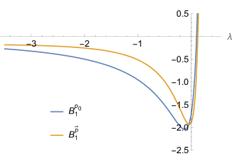
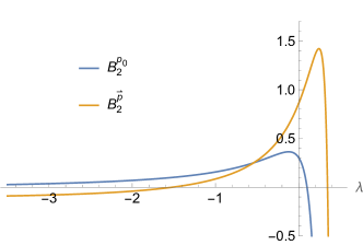
Figure 1: Plots of the functions $B_{1}(\lambda)$ (left) and $B_{2}(\lambda)$ (right) given in Eqs. (28) and (29).

At this stage, a number of observations are in order. First, the functions $B_{1}(\lambda)$ and $B_{2}(\lambda)$ are shown in Fig. 1. From these plots, we find that two projection methods give qualitatively similar results. This suggests that even though the spatial momentum regulator breaks Lorentz symmetry, the qualitative properties of the RG flow are projection independent.

In addition, the analytic structure of $\beta_{\lambda}$ and $\beta_{g}$ warrants a detailed discussion. We start with the locus $\lambda=0$. Fig. 1 shows that $B_{1}(\lambda)$ and $B_{2}(\lambda)$ are regular at $\lambda=0$, despite the poles shown in Eqs. (28) and (29). This feature can also be confirmed analytically by explicitly evaluating the limits of the functions at this point. This property also extends to $\beta_{\lambda}$. As a consequence, the line $\lambda=0$ is regular with respect to the RG flow for generic values $g$. A brief inspection of the numerators appearing in $\beta_{\lambda}$, $B_{1}(\lambda)$, and $B_{2}(\lambda)$ shows that the beta functions exhibit poles of finite order at

$$\begin{split}\gamma_{1}^{\rm sing}\;:&\;\left\{(g,\lambda)\;|\;(\lambda=1/2,g\not=0)\right\}\,,\\ \gamma_{2}^{\rm sing}\;:&\;\left\{(g,\lambda)\;|\;(\lambda=2/3,g\not=0)\right\}\,.\end{split}$$ (30)

These lines constitute singularities of the flow equation that cannot be crossed by its solutions. In addition, there is a singular locus caused by the divergence of $\eta_{N}$. This occurs when the denominator in $\eta_{N}$ vanishes

$$\gamma^{\rm sing}_{3}\;:\;\left\{(g,\lambda)\;|\;g=1/B_{2}(\lambda)\,\right\}\,.$$ (31)

Finally, we observe that $\beta_{\lambda}$, $B_{1}$, and $B_{2}$ contain the combination $(1-2\lambda)$ (and also $(1-3/2\lambda)$) with half-integer powers. This leads to branch cuts

$$\gamma^{\rm cut}\;:\;\left\{(g,\lambda)\;|\;\lambda>1/2\,\right\}\,.$$ (32)

In this region, the arguments of the square roots turn negative so that the beta functions take complex values. The comparison with the beta functions computed in [82] shows that this feature originates from the use of the spatial regulator (21). For a covariant regulator the square roots are absent and there is a well-defined RG flow for $\lambda>1/2$ as well.

V Fixed points and phase diagrams

We proceed by constructing the phase diagrams resulting from the beta functions (26). In addition to the singular lines and branch cuts (30)-(32), the flow is governed by the interplay of its fixed points $(g_{*},\lambda_{*})$ where, by definition $\beta_{g}(g_{*},\lambda_{*})=\beta_{\lambda}(g_{*},\lambda_{*})=0$. The properties of the flow in the vicinity of such a fixed point are then encoded in the stability matrix

$$B_{j}{}^{i}\equiv\left.\frac{\partial\beta_{u^{i}}}{\partial u^{j}}\right|_{u=u_{*}}\,.$$ (33)

Defining the stability coefficients $\theta_{i}$ as minus the eigenvalues of $B$, eigendirections where Re($\theta_{i})>0$ (Re($\theta_{i})<0$) are attracted towards (repelled by) the fixed point as $k\rightarrow\infty$. Hence, UV-attractive eigendirections come with Re($\theta_{i})>0$.

Investigating the fixed points of (26), we first encounter the Gaussian fixed point (GFP),

$$\text{GFP:}\qquad(g_{*},\lambda_{*})=(0,0)\,,\quad(\theta_{1},\theta_{2})=(2,-2).$$ (34)

The stability properties of this fixed point coincide with canonical power counting, warranting its classification as a Gaussian (or non-interacting) fixed point. The GFP is a saddle point. Its UV-repulsive direction is associated with the coupling $g_{k}$, so that trajectories with $g_{k}>0$ are repelled by this fixed point as $k\rightarrow\infty$. In addition to the GFP, the system also possesses a number of non-Gaussian fixed points (NGFPs). These are tabulated in Table 3. One finds three candidate fixed points for the $p_{0}$-projection while the $\vec{p}$-projection gives rise to two roots only. Remarkably, both projection schemes give rise to a NGFP situated at a positive Newton’s coupling coming with two UV-attractive eigendirections. This solution is labeled NGFP₁. Although the numerical values of its position and stability coefficients differ significantly for the two projection schemes, this fixed point shares all properties required for a UV-completion of gravity. NGFP₂ and NGFP₃ are located at $g_{*}<0$. Hence their flow is disconnected from the physically interested region where Newton’s coupling is positive. Thus, these solutions will not play any role in the subsequent discussion.

Projection	. Fixed Points	Couplings		Critical Exponents
		$g_{*}$	. $\lambda_{*}$	$\theta_{1}$	$\theta_{2}$
$p_{0}$	. NGFP1	$0.89$	$-0.40$	$5.44$	$1.25$
	. NGFP2	$-0.17$	$0.21$	$1.96\pm 5.70i$
	. NGFP3	$-818.39$	$-21.94$	$-31.73$	$0.33$
$\vec{p}$	. NGFP1	$301.53$	$-12.55$	$14.11$	$0.30$
	. NGFP2	$-0.14$	$0.25$	$-0.40\pm 5.61i$

Table 3: The fixed-point structures for the analytically continued Einstein-Hilbert truncation with $|\epsilon_{s}|=1$. The relevant fixed point NGFP₁ persists for all projection schemes. While the numerical values of its position and critical exponents differ substantially, all schemes agree on its existence and its two relevant directions. The solutions NGFP₂ and NGFP₃ are added for completeness.

We proceed by presenting the phase diagrams arising from the $p_{0}$- and $\vec{p}$-projections. The focus is on the region $g\geq 0$, $\lambda\leq 1/2$ which is bounded by $\gamma_{2}^{\rm sing}$ to its right. The flow in this region is governed by the interplay of the GFP, NGFP₁, and the singular locus $\gamma_{3}^{\rm sing}$. For the $p_{0}$-projection, the resulting phase diagram is shown in Fig. 2.

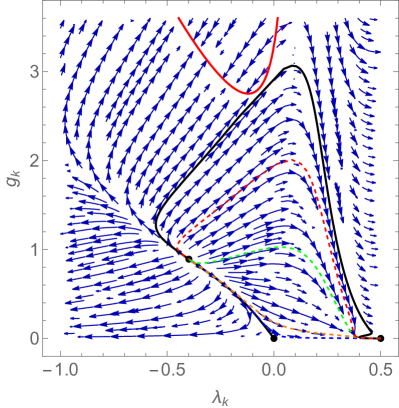
Figure 2: Phase diagram for the Lorentzian Einstein-Hilbert truncation arising from the beta functions of the $p_{0}$-projection. The arrows point towards the lower values of the coarse-graining scale $k$. We mark the GFP (34), the NGFP₁ from Table 3, and the IR-FP (35) with black dots. The red line denotes the singular locus $\gamma^{\rm sing}_{3}$ while the thick black lines label the separatrix and the boundary of the region with RG trajectories connecting NGFP₁ to the IR-FP. The colored dashed lines correspond to the RG trajectories along which we analyze the scaling of the couplings. The scaling behavior along these trajectories can be found in the left column of Fig. 4.

The most remarkable feature revealed by the phase diagram is the presence of an IR-FP

$$\text{IR-FP}:\quad(g_{*}^{\rm IR},\lambda_{*}^{\rm IR})=(0,1/2)\,.$$ (35)

This fixed point escapes the standard search for fixed points since the beta functions are degenerate for these specific values of the couplings. The presence of the fixed point is then concluded based on scaling properties of RG trajectories in its vicinity. A numerical investigation shows that these indeed follow a power-law scaling

$$\text{IR-FP:}\quad\lambda_{*}^{\rm IR}-\lambda_{k}\sim c_{1}e^{1.15t}\,,\;g_{k}-g_{*}^{\rm IR}\sim c_{2}e^{4t}\,.$$ (36)

Here the constants $c_{1}$ and $c_{2}$ specify the RG trajectory and the symbol $\sim$ indicates that Eq. (36) holds in the vicinity of the IR-FP only. Converting back to the dimensionful graviton mass $\mu_{k}^{2}\equiv-2\lambda_{k}\,k^{2}$ shows that this IR-FP entails a vanishing graviton mass in the limit $k\rightarrow 0$.

In the next step, we identify two special RG trajectories, the separatrix connecting the NGFP₁ to the GFP, and the boundary for the trajectories connecting the NGFP₁ to the IR-FP. These are highlighted by the thick black lines. They bound the region in phase space where the trajectories end up in the IR-FP as $k\rightarrow 0$. These trajectories then exhibit a vanishing renormalized graviton mass. In addition to this phase, there is a set of RG trajectories to the left of the separatrix. These either terminate in $\gamma_{3}^{\rm sing}$ at a finite value of $k$ or reach the endpoint $(g,\lambda)=(0,-\infty)$ at $k=0$. The latter correspond to RG trajectories with a positive renormalized graviton mass.

The analogous analysis for the $\vec{p}$-projection is summarized in Fig. 3.

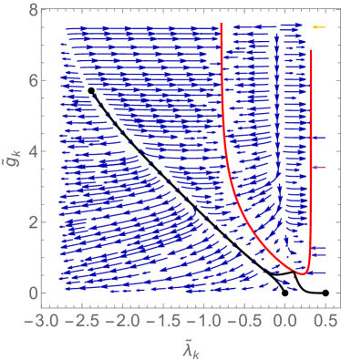
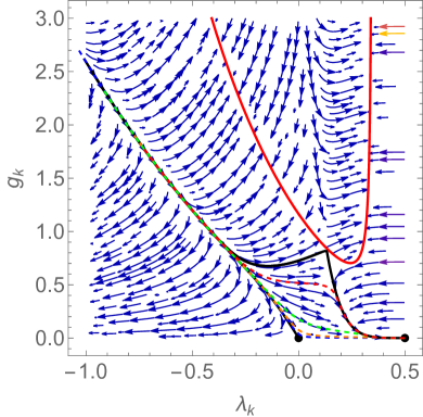
Figure 3: Phase diagrams for the Lorentzian Einstein-Hilbert truncation based on the $\vec{p}$-projection. The left diagram shows the global properties of the flow, utilizing the map (37). The right diagram zooms into the part showing the interplay of the GFP, IR-FP, together with RG trajectories emanating from the NGFP₁. The arrows point towards the lower values of the coarse-graining scale $k$. The GFP (34), the NGFP₁ from Table 3, and the IR-FP are marked by black dots. The red line denotes the singular locus $\gamma^{\rm sing}_{3}$ while the thick black lines label the separatrix and the boundary of the region with RG trajectories connecting NGFP₁ to the IR-FP. The colored dashed lines correspond to the RG trajectories along which we analyze the scaling of the couplings displayed in the right column of Fig. 4.

In this case, the NGFP₁ is located at $(g_{*},\lambda_{*})=(301.53,-12.55)$. In order to be able to capture all relevant features of the phase diagram, we use the following redefinition of the couplings

$$\tilde{g}_{k}=\text{ln}(g_{k}+1),\quad\tilde{\lambda}_{k}=-\text{ln}(\lambda_{c}-\lambda_{k})+\text{ln}\lambda_{c}\,.$$ (37)

The constant $\lambda_{c}$ is chosen as $\lambda_{c}=1/(2-2~e^{-1/2})$ which ensures that the positions of the GFP and IR-FP remain the same also in the new couplings. The phase diagram for the global flow is then obtained from the beta functions $(\beta_{\tilde{g}}(\tilde{g},\tilde{\lambda}),\beta_{\tilde{\lambda}}(\tilde{g},\tilde{\lambda}))$ and shown in the left panel of Fig. 3. The right panel uses the original coordinates $(g_{k},\lambda_{k})$ and zooms into the lower-right corner thereby highlighting the interplay between the GFP, IR-FP and $\gamma_{3}^{\rm sing}$. Notably, the phase diagram is qualitatively identical to the one shown in Fig. 2. In particular, the IR-FP is again located at (35) and induces the characteristic scaling (36) for RG trajectories in its vicinity. The new feature is the long funnel connecting the lower-right region to the NGFP₁. Essentially, the RG trajectories emanating from NGFP₁ and reaching this region are squeezed into an extremely narrow shape which can be almost regarded as a line.

We complete the discussion of the phase diagrams by displaying the dependence of $\lambda_{k}$ on the RG time $t=\text{ln}(k/k_{0})$ along the RG trajectories highlighted in Figs. 2 and 3. The result is shown in Fig. 4. All curves interpolate between the NGFP₁ in the limit $t\rightarrow\infty$ and the IR-FP as $t\rightarrow-\infty$. The logarithmic plots showing the $k$-dependence of the dimensionful coupling $\Lambda_{k}$ establish that the IR-FP implies $\lim_{t\rightarrow-\infty}\Lambda_{k}=0$. The scaling laws (36) can be verified by tracking the convergence of $\lambda_{k}$ towards $\lambda_{*}^{\rm IR}$ using a logarithmic scale for the difference.

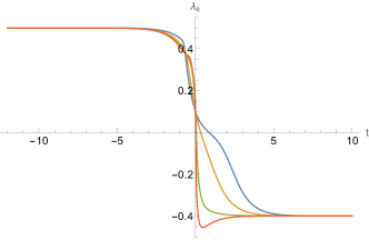
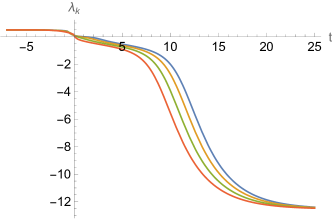
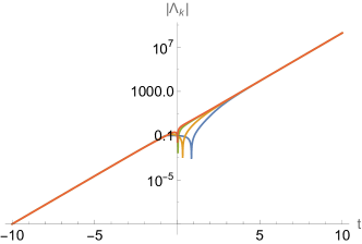
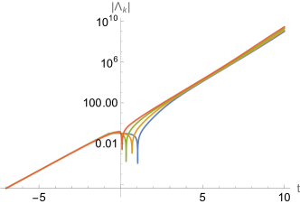
Figure 4: Examples illustrating the $t$-dependence of the dimensionless coupling $\lambda_{k}$ (top line) and its dimensionful counterpart $\Lambda_{k}$ (bottom line) along the colored RG trajectories shown in Fig. 2 ($p_{0}$-projection; left column) and Fig. 3 ($\vec{p}$-projection; right column). For $t\gg 1$ the flow is controlled by the NGFP₁ and $\lambda_{k}$ converges to its fixed point value $\lambda_{*}$ as $t\rightarrow\infty$. As $t$ decreases, we find a region near the GFP where the dimensionful coupling $\Lambda_{k}$ behaves like a constant. In this region one also observes the spikes in $|\Lambda_{k}|$ which reflect the change of its sign in a logarithmic representation. For $t\rightarrow-\infty$, the trajectories approach the IR-FP. The feature that the IR-FP drives the dimensionful $\Lambda_{k}$ to zero is then readily seen from the diagrams in the bottom row.

We close this section with an important remark. We recall [96, 3] that predictions based on the asymptotic safety mechanism should be based on renormalized couplings. These are obtained at the endpoint of an RG trajectory in the limit $k=0$ where all quantum corrections have been taken into account. Applying this philosophy to the phase diagrams obtained from the $p_{0}$-projection and the $\vec{p}$-projection reveals an astonishing feature: despite the apparent differences in Figs. 2 and 3 their predictions are actually identical: the values for $\Lambda_{k}$ compatible with Asymptotic Safety provided by NGFP₁ are

$$\Lambda_{0}\leq 0\,,$$ (38)

with $\Lambda_{0}=0$ related to the IR-FP attractor. In other words, the squared mass appearing in the Lorentzian graviton propagator given in the first line of Table 1 may either be positive or zero. The latter case arises from an attractor mechanism without the need of fine-tuning initial conditions to a fixed value. We find it remarkable that both Lorentzian and Euclidean signature computations carried out in this work agree on this feature.

VI Summary and Outlook

The transition from Euclidean to Lorentzian signature is a key step in developing the gravitational asymptotic safety program. In comparison to the Euclidean setting, Lorentzian signature computations require an additional geometric structure: a preferred direction which serves as time. Our work implements this structure via the ADM decomposition of the metric field. Our focus is then on the connection of the Euclidean and Lorentzian settings through the analytic continuation of the lapse function (3). This setting is used to determine the flow of the graviton two-point function with the propagator and interactions extracted from the gauge-fixed Einstein-Hilbert action. We explicitly establish that the Lorentzian two-point function resulting from the analytic continuation has the causal structure of the Feynman propagator. Moreover, it is shown that the beta functions obtained from the Lorentzian and Euclidean signature computations are identical. A key ingredient underlying these results is the choice of a spatial regulator (21) which renders loop-computations finite without introducing new poles in the complex momentum plane. These properties come at the expense that the regulator breaks Lorentz covariance explicitly. Notably, this is the first time that a two-point function of an ADM field has been computed in the Lorentzian signature setting.

The phase diagrams determining the flow of the graviton mass with respect to the coarse-graining scale are given in Figs. 2 and 3. Since the ADM decomposition allows to distinguish between spatial and time-components of the external momentum, the flow diagram can be constructed by reading off the wave function renormalization from the time-part ($p_{0}$-projection) or the spatial components ($\vec{p}$-projection) of the external four-momentum. Both projections give rise to a non-Gaussian renormalization group fixed point suitable for Asymptotic Safety. In the $\vec{p}$-projection the position of the fixed point is shifted substantially. A direct comparison with the fixed point results reported for a covariant regulator [82] indicates that this shift is due to the spatial momentum regulator adopted in this work. Nevertheless, the phase diagrams are qualitatively similar and agree on their predictions for the graviton mass compatible with Asymptotic Safety. Moreover, the phase diagrams capturing the flow at Lorentzian signature agree with the ones found for the ADM decomposition [82] and the covariant setting [19], carried out in a Euclidean background. In particular, the IR-attractor driving the graviton mass to zero dynamically operates in all cases.

It would be interesting to extend the results reported in this work in various ways. First, one could extend the momentum dependence of the graviton two-point function tracked in our work by promoting the $p^{2}$-term to a form factor $f(p^{2})$, capturing the full momentum dependence along the lines [97, 98, 5, 99, 68, 69]. The flow equation should then determine the analytic structure of the propagator including potential poles in the complex momentum plane. Equivalence of the Euclidean and Lorentzian setting at the level of form factors then requires that this generalization does not lead to new poles in the complex momentum plane with are crossed when performing the analytic continuation of the lapse function. This property is highly non-trivial and should be established based on explicit computations.

Second, it would be interesting to find a Lorentz-covariant way to carry out computations within the ADM formalism. Notably, the spatial momentum regulator is not the only ingredient giving rise to Lorentz symmetry breaking contributions to the RG flow [82]. At this stage, the construction of a Lorentz-covariant flow on a foliated spacetime, using a covariant regulator, would be desirable. Such a construction requires a non-linear field redefinition of the ADM fields [83]. Similarly to the definition of the fluctuation field based on the linear and exponential split in covariant computations [100], such a redefinition of the fluctuation field may lead to new properties in the RG flow that signal that ultimately, one is quantizing a different theory. We will return to this point in future work [101].

Finally, the present computation is readily generalized to other two-point functions. In this context, the two-point function of the trace mode may be of special interest since this may be related to correlation functions measured within the Causal Dynamical Triangulations program [102, 103] along the lines [104]. Considering that the trace correlator may depend on the gauge condition, one may need the method developed in [105] combining the Quantum Master Equation and Wilsonian RG flow equation to extract the BRST-invariant flow. This will also be considered in future work.

Appendix A The ghost sector

The ghost term appearing in Eq. (14) is conveniently split into a scalar and vector part

$$\Gamma^{\text{ghost}}=\Gamma_{\text{scalar}}^{\text{ghost}}+\Gamma_{\text{vec}}^{\text{ghost}}\,.$$ (39)

The Faddeev-Popov procedure yields

$$\begin{split}\Gamma_{\text{scalar}}^{\text{ghost}}=&\int d\tau d^{3}y\,\sqrt{\epsilon_{s}}\,\bar{c}\,[\partial_{\tau}^{2}cN+\partial_{\tau}b^{k}\partial_{k}N-\partial_{\tau}NN_{j}\sigma^{ij}\partial_{i}c\\ &+\partial^{i}\partial_{\tau}N_{i}c+\partial^{i}b^{k}\partial_{k}N_{i}+\partial^{i}N_{k}\partial_{i}b^{k}+\partial^{i}\sigma_{ki}\partial_{\tau}b^{k}\\ &-\partial_{\tau}\sigma_{ik}\partial^{i}b^{k}+\partial^{i}\sigma^{kl}N_{k}N_{l}\partial_{i}c+\epsilon_{s}\partial^{i}N^{2}\partial_{i}c\\ &-\frac{1}{{2}}~\partial_{\tau}c\partial_{\tau}\bar{\sigma}^{ij}\sigma_{ij}-\frac{1}{{2}}\partial_{\tau}b^{k}\partial_{k}\bar{\sigma}^{ij}\sigma_{ij}-\partial_{\tau}N^{i}\partial_{i}c],\end{split}$$ (40)

and

$$\begin{split}\Gamma_{\text{vec}}^{\text{ghost}}=&\int d\tau d^{3}y\,\sqrt{\epsilon_{s}}\,\bar{b}^{i}\,\Big{[}\frac{1}{\epsilon_{s}}\partial^{2}_{\tau}N_{i}c+\frac{1}{\epsilon_{s}}\partial_{\tau}\sigma^{kl}N_{k}N_{l}\partial_{i}c\\ &+\partial_{\tau}N^{2}\partial_{i}c-\partial_{i}\partial_{\tau}Nc-\partial_{i}N_{m}\partial^{m}c\\ &+\partial_{i}NN_{k}\sigma^{kl}\partial_{l}c+\partial^{j}N_{i}\partial_{j}c+\partial^{j}N_{j}\partial_{i}c\\ &-\frac{1}{2}\partial_{i}c\partial_{\tau}\delta^{mn}\sigma_{mn}+\partial^{j}c\partial_{\tau}\sigma_{ij}+\frac{1}{\epsilon_{s}}\partial_{\tau}b^{k}\partial_{k}N_{i}\\ &+\frac{1}{\epsilon_{s}}\partial_{\tau}N_{k}\partial_{i}b^{k}+\frac{1}{\epsilon_{s}}\partial_{\tau}\sigma_{ki}\partial_{\tau}b^{k}-\partial_{i}b^{k}\partial_{k}N\\ &-\frac{1}{2}\partial_{i}b^{k}\partial_{k}\delta^{mn}\sigma_{mn}-\partial_{i}\sigma_{jk}\partial^{j}b^{k}+\partial^{j}b^{k}\partial_{k}\sigma_{ij}\\ &+\partial^{j}\sigma_{jk}\partial_{i}b^{k}+\partial^{j}\sigma_{ik}\partial_{j}b^{k}\Big{]}.\end{split}$$ (41)

Here all derivatives act on the right, for instance, $\partial_{\tau}N_{i}c=N_{i}(\partial_{\tau}c)+(\partial_{\tau}N_{i})c$. In addition, all indices are raised and lowered with the flat background metric $\delta_{ij}$.

References

- [1] R. Percacci, An Introduction to Covariant Quantum Gravity and Asymptotic Safety, Vol. 3 of 100 Years of General Relativity, World Scientific, 2017. doi:10.1142/10369.
- [2] M. Reuter, F. Saueressig, Quantum Gravity and the Functional Renormalization Group: The Road towards Asymptotic Safety, Cambridge University Press, 2019.
- [3] F. Saueressig, The Functional Renormalization Group in Quantum Gravity, 2023. arXiv:2302.14152, doi:10.1007/978-981-19-3079-9_16-1.
- [4] J. M. Pawlowski, M. Reichert, Quantum Gravity from dynamical metric fluctuations (9 2023). arXiv:2309.10785.
- [5] B. Knorr, C. Ripken, F. Saueressig, Form Factors in Asymptotically Safe Quantum Gravity, 2024. arXiv:2210.16072, doi:10.1007/978-981-19-3079-9_21-1.
- [6] T. R. Morris, D. Stulga, The Functional f(R) Approximation, 2023. arXiv:2210.11356, doi:10.1007/978-981-19-3079-9_19-1.
- [7] R. Martini, G. P. Vacca, O. Zanusso, Perturbative Approaches to Nonperturbative Quantum Gravity, 2024, pp. 1–46. arXiv:2210.13910, doi:10.1007/978-981-19-3079-9_25-1.
- [8] C. Wetterich, Quantum Gravity and Scale Symmetry in Cosmology, 2023. arXiv:2211.03596, doi:10.1007/978-981-19-3079-9_26-1.
- [9] A. Codello, R. Percacci, C. Rahmede, Investigating the Ultraviolet Properties of Gravity with a Wilsonian Renormalization Group Equation, Annals Phys. 324 (2009) 414–469. arXiv:0805.2909, doi:10.1016/j.aop.2008.08.008.
- [10] S. Nagy, Lectures on renormalization and asymptotic safety, Annals Phys. 350 (2014) 310–346. arXiv:1211.4151, doi:10.1016/j.aop.2014.07.027.
- [11] M. Reichert, Lecture notes: Functional Renormalisation Group and Asymptotically Safe Quantum Gravity, PoS 384 (2020) 005. doi:10.22323/1.384.0005.
- [12] S. Weinberg, Ultraviolet divergences in quantum theories of gravitation, General Relativity: An Einstein centenary survey, Eds. Hawking, S.W., Israel, W; Cambridge University Press (1979) 790–831.
- [13] C. Wetterich, Exact evolution equation for the effective potential, Phys. Lett. B 301 (1993) 90–94. arXiv:1710.05815, doi:10.1016/0370-2693(93)90726-X.
- [14] T. R. Morris, The Exact renormalization group and approximate solutions, Int. J. Mod. Phys. A 9 (1994) 2411–2450. arXiv:hep-ph/9308265, doi:10.1142/S0217751X94000972.
- [15] M. Reuter, Nonperturbative evolution equation for quantum gravity, Phys. Rev. D 57 (1998) 971–985. arXiv:hep-th/9605030, doi:10.1103/PhysRevD.57.971.
- [16] N. Christiansen, K. Falls, J. M. Pawlowski, M. Reichert, Curvature dependence of quantum gravity, Phys. Rev. D 97 (4) (2018) 046007. arXiv:1711.09259, doi:10.1103/PhysRevD.97.046007.
- [17] T. Denz, J. M. Pawlowski, M. Reichert, Towards apparent convergence in asymptotically safe quantum gravity, Eur. Phys. J. C 78 (4) (2018) 336. arXiv:1612.07315, doi:10.1140/epjc/s10052-018-5806-0.
- [18] N. Christiansen, B. Knorr, J. Meibohm, J. M. Pawlowski, M. Reichert, Local Quantum Gravity, Phys. Rev. D 92 (12) (2015) 121501. arXiv:1506.07016, doi:10.1103/PhysRevD.92.121501.
- [19] N. Christiansen, B. Knorr, J. M. Pawlowski, A. Rodigast, Global Flows in Quantum Gravity, Phys. Rev. D 93 (4) (2016) 044036. arXiv:1403.1232, doi:10.1103/PhysRevD.93.044036.
- [20] A. Eichhorn, The Renormalization Group flow of unimodular f(R) gravity, JHEP 04 (2015) 096. arXiv:1501.05848, doi:10.1007/JHEP04(2015)096.
- [21] H. Gies, A. S. Salek, Asymptotically safe Hilbert–Palatini gravity in an on-shell reduction scheme, Eur. Phys. J. C 83 (2) (2023) 173. arXiv:2209.10435, doi:10.1140/epjc/s10052-023-11324-1.
- [22] H. Gies, B. Knorr, S. Lippoldt, F. Saueressig, Gravitational Two-Loop Counterterm Is Asymptotically Safe, Phys. Rev. Lett. 116 (21) (2016) 211302. arXiv:1601.01800, doi:10.1103/PhysRevLett.116.211302.
- [23] G. P. de Brito, A. D. Pereira, A. F. Vieira, Exploring new corners of asymptotically safe unimodular quantum gravity, Phys. Rev. D 103 (10) (2021) 104023. arXiv:2012.08904, doi:10.1103/PhysRevD.103.104023.
- [24] G. P. De Brito, N. Ohta, A. D. Pereira, A. A. Tomaz, M. Yamada, Asymptotic safety and field parametrization dependence in the truncation, Phys. Rev. D 98 (2) (2018) 026027. arXiv:1805.09656, doi:10.1103/PhysRevD.98.026027.
- [25] Y. Kluth, D. F. Litim, Functional renormalization for f(R) quantum gravity, Phys. Rev. D 106 (10) (2022) 106022. arXiv:2202.10436, doi:10.1103/PhysRevD.106.106022.
- [26] A. Pastor-Gutiérrez, J. M. Pawlowski, M. Reichert, The Asymptotically Safe Standard Model: From quantum gravity to dynamical chiral symmetry breaking, SciPost Phys. 15 (3) (2023) 105. arXiv:2207.09817, doi:10.21468/SciPostPhys.15.3.105.
- [27] B. Bürger, J. M. Pawlowski, M. Reichert, B.-J. Schaefer, Curvature dependence of quantum gravity with scalars (12 2019). arXiv:1912.01624.
- [28] J. M. Pawlowski, M. Reichert, C. Wetterich, M. Yamada, Higgs scalar potential in asymptotically safe quantum gravity, Phys. Rev. D 99 (8) (2019) 086010. arXiv:1811.11706, doi:10.1103/PhysRevD.99.086010.
- [29] A. Eichhorn, S. Lippoldt, J. M. Pawlowski, M. Reichert, M. Schiffer, How perturbative is quantum gravity?, Phys. Lett. B 792 (2019) 310–314. arXiv:1810.02828, doi:10.1016/j.physletb.2019.01.071.
- [30] A. Eichhorn, P. Labus, J. M. Pawlowski, M. Reichert, Effective universality in quantum gravity, SciPost Phys. 5 (4) (2018) 031. arXiv:1804.00012, doi:10.21468/SciPostPhys.5.4.031.
- [31] N. Christiansen, D. F. Litim, J. M. Pawlowski, M. Reichert, Asymptotic safety of gravity with matter, Phys. Rev. D 97 (10) (2018) 106012. arXiv:1710.04669, doi:10.1103/PhysRevD.97.106012.
- [32] J. Meibohm, J. M. Pawlowski, Chiral fermions in asymptotically safe quantum gravity, Eur. Phys. J. C 76 (5) (2016) 285. arXiv:1601.04597, doi:10.1140/epjc/s10052-016-4132-7.
- [33] J. Meibohm, J. M. Pawlowski, M. Reichert, Asymptotic safety of gravity-matter systems, Phys. Rev. D 93 (8) (2016) 084035. arXiv:1510.07018, doi:10.1103/PhysRevD.93.084035.
- [34] G. P. de Brito, A. Eichhorn, Nonvanishing gravitational contribution to matter beta functions for vanishing dimensionful regulators, Eur. Phys. J. C 83 (2) (2023) 161. arXiv:2201.11402, doi:10.1140/epjc/s10052-023-11172-z.
- [35] A. Eichhorn, J. H. Kwapisz, M. Schiffer, Weak-gravity bound in asymptotically safe gravity-gauge systems, Phys. Rev. D 105 (10) (2022) 106022. arXiv:2112.09772, doi:10.1103/PhysRevD.105.106022.
- [36] G. P. de Brito, A. Eichhorn, R. R. L. d. Santos, The weak-gravity bound and the need for spin in asymptotically safe matter-gravity models, JHEP 11 (2021) 110. arXiv:2107.03839, doi:10.1007/JHEP11(2021)110.
- [37] G. P. de Brito, A. Eichhorn, M. Schiffer, Light charged fermions in quantum gravity, Phys. Lett. B 815 (2021) 136128. arXiv:2010.00605, doi:10.1016/j.physletb.2021.136128.
- [38] A. Eichhorn, A. Platania, M. Schiffer, Lorentz invariance violations in the interplay of quantum gravity with matter, Phys. Rev. D 102 (2) (2020) 026007. arXiv:1911.10066, doi:10.1103/PhysRevD.102.026007.
- [39] A. Eichhorn, S. Lippoldt, M. Schiffer, Zooming in on fermions and quantum gravity, Phys. Rev. D 99 (8) (2019) 086002. arXiv:1812.08782, doi:10.1103/PhysRevD.99.086002.
- [40] A. Eichhorn, A. Held, Mass difference for charged quarks from asymptotically safe quantum gravity, Phys. Rev. Lett. 121 (15) (2018) 151302. arXiv:1803.04027, doi:10.1103/PhysRevLett.121.151302.
- [41] A. Eichhorn, Y. Hamada, J. Lumma, M. Yamada, Quantum gravity fluctuations flatten the Planck-scale Higgs potential, Phys. Rev. D 97 (8) (2018) 086004. arXiv:1712.00319, doi:10.1103/PhysRevD.97.086004.
- [42] A. Eichhorn, A. Held, Top mass from asymptotic safety, Phys. Lett. B 777 (2018) 217–221. arXiv:1707.01107, doi:10.1016/j.physletb.2017.12.040.
- [43] P. Donà, A. Eichhorn, P. Labus, R. Percacci, Asymptotic safety in an interacting system of gravity and scalar matter, Phys. Rev. D 93 (4) (2016) 044049, [Erratum: Phys.Rev.D 93, 129904 (2016)]. arXiv:1512.01589, doi:10.1103/PhysRevD.93.129904.
- [44] B. Knorr, Safe essential scalar-tensor theories (4 2022). arXiv:2204.08564.
- [45] G. P. De Brito, Y. Hamada, A. D. Pereira, M. Yamada, On the impact of Majorana masses in gravity-matter systems, JHEP 08 (2019) 142. arXiv:1905.11114, doi:10.1007/JHEP08(2019)142.
- [46] A. Eichhorn, M. Schiffer, Asymptotic safety of gravity with matter (12 2022). arXiv:2212.07456.
- [47] A. Eichhorn, A. Held, Black holes in asymptotically safe gravity and beyond (12 2022). arXiv:2212.09495.
- [48] A. Platania, Black Holes in Asymptotically Safe Gravity, 2023. arXiv:2302.04272, doi:10.1007/978-981-19-3079-9_24-1.
- [49] A. Bonanno, F. Saueressig, Asymptotically safe cosmology – A status report, Comptes Rendus Physique 18 (2017) 254–264. arXiv:1702.04137, doi:10.1016/j.crhy.2017.02.002.
- [50] A. Bonanno, Asymptotic Safety and Cosmology, 2024. doi:10.1007/978-981-19-3079-9_23-1.
- [51] J. Ambjørn, J. Gizbert-Studnicki, A. Gőrlich, D. Németh, Is lattice quantum gravity asymptotically safe? Making contact between causal dynamical triangulations and the functional renormalization group, Phys. Rev. D 110 (12) (2024) 126006. arXiv:2408.07808, doi:10.1103/PhysRevD.110.126006.
- [52] J. Ambjorn, J. Gizbert-Studnicki, A. Goerlich, D. Nemeth, IR and UV limits of CDT and their relations to FRG (11 2024). arXiv:2411.02330.
- [53] T. Thiemann, Asymptotically safe — canonical quantum gravity junction, JHEP 10 (2024) 013. arXiv:2404.18220, doi:10.1007/JHEP10(2024)013.
- [54] R. Ferrero, T. Thiemann, Relational Lorentzian Asymptotically Safe Quantum Gravity: Showcase Model, Universe 10 (11) (2024) 410. arXiv:2404.18224, doi:10.3390/universe10110410.
- [55] I. Basile, A. Platania, Asymptotic Safety: Swampland or Wonderland?, Universe 7 (10) (2021) 389. arXiv:2107.06897, doi:10.3390/universe7100389.
- [56] B. Knorr, A. Platania, Unearthing the intersections: positivity bounds, weak gravity conjecture, and asymptotic safety landscapes from photon-graviton flows (5 2024). arXiv:2405.08860.
- [57] A. Eichhorn, A. O. Pedersen, M. Schiffer, Application of positivity bounds in asymptotically safe gravity (5 2024). arXiv:2405.08862.
- [58] A. Eichhorn, A. Hebecker, J. M. Pawlowski, J. Walcher, The Absolute Swampland (5 2024). arXiv:2405.20386.
- [59] N. D. Birrell, P. C. W. Davies, Quantum Fields in Curved Space, Cambridge Monographs on Mathematical Physics, Cambridge University Press, Cambridge, UK, 1982. doi:10.1017/CBO9780511622632.
- [60] M. Demmel, A. Nink, Connections and geodesics in the space of metrics, Phys. Rev. D 92 (10) (2015) 104013. arXiv:1506.03809, doi:10.1103/PhysRevD.92.104013.
- [61] A. Baldazzi, R. Percacci, V. Skrinjar, Wicked metrics, Class. Quant. Grav. 36 (10) (2019) 105008. arXiv:1811.03369, doi:10.1088/1361-6382/ab187d.
- [62] E. Manrique, S. Rechenberger, F. Saueressig, Asymptotically Safe Lorentzian Gravity, Phys. Rev. Lett. 106 (2011) 251302. arXiv:1102.5012, doi:10.1103/PhysRevLett.106.251302.
- [63] E. D’Angelo, N. Drago, N. Pinamonti, K. Rejzner, An Algebraic QFT Approach to the Wetterich Equation on Lorentzian Manifolds, Annales Henri Poincare 25 (4) (2024) 2295–2352. arXiv:2202.07580, doi:10.1007/s00023-023-01348-4.
- [64] E. D’Angelo, K. Rejzner, A Lorentzian renormalisation group equation for gauge theories (3 2023). arXiv:2303.01479.
- [65] E. D’Angelo, Asymptotic safety in Lorentzian quantum gravity, Phys. Rev. D 109 (6) (2024) 066012. arXiv:2310.20603, doi:10.1103/PhysRevD.109.066012.
- [66] R. Banerjee, M. Niedermaier, The spatial Functional Renormalization Group and Hadamard states on cosmological spacetimes, Nucl. Phys. B 980 (2022) 115814. arXiv:2201.02575, doi:10.1016/j.nuclphysb.2022.115814.
- [67] R. Banerjee, M. Niedermaier, Wick rotation in the lapse: admissible complex metrics and the associated heat kernel (6 2024). arXiv:2406.06047.
- [68] A. Bonanno, T. Denz, J. M. Pawlowski, M. Reichert, Reconstructing the graviton, SciPost Phys. 12 (1) (2022) 001. arXiv:2102.02217, doi:10.21468/SciPostPhys.12.1.001.
- [69] J. Fehre, D. F. Litim, J. M. Pawlowski, M. Reichert, Lorentzian Quantum Gravity and the Graviton Spectral Function, Phys. Rev. Lett. 130 (8) (2023) 081501. arXiv:2111.13232, doi:10.1103/PhysRevLett.130.081501.
- [70] J. Ambjorn, A. Goerlich, J. Jurkiewicz, R. Loll, Nonperturbative Quantum Gravity, Phys. Rept. 519 (2012) 127–210. arXiv:1203.3591, doi:10.1016/j.physrep.2012.03.007.
- [71] R. Loll, Quantum Gravity from Causal Dynamical Triangulations: A Review, Class. Quant. Grav. 37 (1) (2020) 013002. arXiv:1905.08669, doi:10.1088/1361-6382/ab57c7.
- [72] J. Ambjørn, R. Loll, Causal Dynamical Triangulations: Gateway to Nonperturbative Quantum Gravity, 2024. arXiv:2401.09399.
- [73] P. Horava, Quantum Gravity at a Lifshitz Point, Phys. Rev. D 79 (2009) 084008. arXiv:0901.3775, doi:10.1103/PhysRevD.79.084008.
- [74] A. O. Barvinsky, D. Blas, M. Herrero-Valea, S. M. Sibiryakov, C. F. Steinwachs, Renormalization of Hořava gravity, Phys. Rev. D 93 (6) (2016) 064022. arXiv:1512.02250, doi:10.1103/PhysRevD.93.064022.
- [75] A. O. Barvinsky, A. V. Kurov, S. M. Sibiryakov, Beta functions of (3+1)-dimensional projectable Hořava gravity, Phys. Rev. D 105 (4) (2022) 044009. arXiv:2110.14688, doi:10.1103/PhysRevD.105.044009.
- [76] A. O. Barvinsky, A. V. Kurov, S. M. Sibiryakov, Asymptotic freedom in (3+1)-dimensional projectable Hořava gravity: Connecting the ultraviolet and infrared domains, Phys. Rev. D 108 (12) (2023) L121503. arXiv:2310.07841, doi:10.1103/PhysRevD.108.L121503.
- [77] R. L. Arnowitt, S. Deser, C. W. Misner, The Dynamics of general relativity, Gen. Rel. Grav. 40 (2008) 1997–2027. arXiv:gr-qc/0405109, doi:10.1007/s10714-008-0661-1.
- [78] E. Gourgoulhon, 3+1 formalism and bases of numerical relativity (3 2007). arXiv:gr-qc/0703035.
- [79] B. Knorr, Lorentz symmetry is relevant, Phys. Lett. B 792 (2019) 142–148. arXiv:1810.07971, doi:10.1016/j.physletb.2019.01.070.
- [80] J. Biemans, A. Platania, F. Saueressig, Quantum gravity on foliated spacetimes: Asymptotically safe and sound, Phys. Rev. D 95 (8) (2017) 086013. arXiv:1609.04813, doi:10.1103/PhysRevD.95.086013.
- [81] J. Biemans, A. Platania, F. Saueressig, Renormalization group fixed points of foliated gravity-matter systems, JHEP 05 (2017) 093. arXiv:1702.06539, doi:10.1007/JHEP05(2017)093.
- [82] F. Saueressig, J. Wang, Foliated asymptotically safe gravity in the fluctuation approach, JHEP 09 (2023) 064. arXiv:2306.10408, doi:10.1007/JHEP09(2023)064.
- [83] G. Korver, F. Saueressig, J. Wang, Global flows of foliated gravity-matter systems, Phys. Lett. B 855 (2024) 138789. arXiv:2402.01260, doi:10.1016/j.physletb.2024.138789.
- [84] C. Wetterich, Simplified functional flow equation (3 2024). arXiv:2403.17523.
- [85] S. Rechenberger, F. Saueressig, A functional renormalization group equation for foliated spacetimes, JHEP 03 (2013) 010. arXiv:1212.5114, doi:10.1007/JHEP03(2013)010.
- [86] J. W. York, Jr., Conformally invariant orthogonal decomposition of symmetric tensors on Riemannian manifolds and the initial value problem of general relativity, J. Math. Phys. 14 (1973) 456–464. doi:10.1063/1.1666338.
- [87] W. B. Houthoff, A. Kurov, F. Saueressig, Impact of topology in foliated Quantum Einstein Gravity, Eur. Phys. J. C 77 (2017) 491. arXiv:1705.01848, doi:10.1140/epjc/s10052-017-5046-8.
- [88] J. M. Bardeen, Gauge Invariant Cosmological Perturbations, Phys. Rev. D 22 (1980) 1882–1905. doi:10.1103/PhysRevD.22.1882.
- [89] B. Craps, T. De Jonckheere, A. S. Koshelev, Cosmological perturbations in non-local higher-derivative gravity, JCAP 11 (2014) 022. arXiv:1407.4982, doi:10.1088/1475-7516/2014/11/022.
- [90] J. M. Pawlowski, M. Reichert, Quantum Gravity: A Fluctuating Point of View, Front. in Phys. 8 (2021) 551848. arXiv:2007.10353, doi:10.3389/fphy.2020.551848.
- [91] J. M. Martin-Garcia, t. . et. al.,̈ http://xact.es/ (2002-2013).
- [92] T. Nutma, xTras : A field-theory inspired xAct package for mathematica, Comput. Phys. Commun. 185 (2014) 1719–1738. arXiv:1308.3493, doi:10.1016/j.cpc.2014.02.006.
- [93] J. Braun, et al., Renormalised spectral flows, SciPost Phys. Core 6 (2023) 061. arXiv:2206.10232, doi:10.21468/SciPostPhysCore.6.3.061.
- [94] D. F. Litim, Optimization of the exact renormalization group, Phys. Lett. B 486 (2000) 92–99. arXiv:hep-th/0005245, doi:10.1016/S0370-2693(00)00748-6.
- [95] D. F. Litim, Optimized renormalization group flows, Phys. Rev. D 64 (2001) 105007. arXiv:hep-th/0103195, doi:10.1103/PhysRevD.64.105007.
- [96] A. Bonanno, A. Eichhorn, H. Gies, J. M. Pawlowski, R. Percacci, M. Reuter, F. Saueressig, G. P. Vacca, Critical reflections on asymptotically safe gravity, Front. in Phys. 8 (2020) 269. arXiv:2004.06810, doi:10.3389/fphy.2020.00269.
- [97] L. Bosma, B. Knorr, F. Saueressig, Resolving Spacetime Singularities within Asymptotic Safety, Phys. Rev. Lett. 123 (10) (2019) 101301. arXiv:1904.04845, doi:10.1103/PhysRevLett.123.101301.
- [98] B. Knorr, C. Ripken, F. Saueressig, Form Factors in Asymptotic Safety: conceptual ideas and computational toolbox, Class. Quant. Grav. 36 (23) (2019) 234001. arXiv:1907.02903, doi:10.1088/1361-6382/ab4a53.
- [99] B. Knorr, C. Ripken, F. Saueressig, Form Factors in Quantum Gravity: Contrasting non-local, ghost-free gravity and Asymptotic Safety, Nuovo Cim. C 45 (2) (2022) 28. arXiv:2111.12365, doi:10.1393/ncc/i2022-22028-5.
- [100] N. Ohta, R. Percacci, A. D. Pereira, Gauges and functional measures in quantum gravity I: Einstein theory, JHEP 06 (2016) 115. arXiv:1605.00454, doi:10.1007/JHEP06(2016)115.
- [101] F. Saueressig, J. Wang, Covariant fluctuations on foliated spacetime, in preparation.
- [102] J. Ambjorn, A. Gorlich, J. Jurkiewicz, R. Loll, The Nonperturbative Quantum de Sitter Universe, Phys. Rev. D 78 (2008) 063544. arXiv:0807.4481, doi:10.1103/PhysRevD.78.063544.
- [103] J. Ambjørn, Z. Drogosz, J. Gizbert-Studnicki, A. Görlich, J. Jurkiewicz, D. Nemeth, Impact of topology in causal dynamical triangulations quantum gravity, Phys. Rev. D 94 (4) (2016) 044010. arXiv:1604.08786, doi:10.1103/PhysRevD.94.044010.
- [104] B. Knorr, F. Saueressig, Towards reconstructing the quantum effective action of gravity, Phys. Rev. Lett. 121 (16) (2018) 161304. arXiv:1804.03846, doi:10.1103/PhysRevLett.121.161304.
- [105] Y. Igarashi, K. Itoh, T. R. Morris, BRST in the exact renormalization group, PTEP 2019 (10) (2019) 103B01. arXiv:1904.08231, doi:10.1093/ptep/ptz099.