Strong Gravitational Lensing by Compact Object without Cauchy Horizons in Effective Quantum Gravity

Abstract

In this work, we study strong gravitational lensing effects of a static, spherically symmetric solution in the context of effective quantum gravity (EQG). Among the three types of solutions proposed in EQG backgrounds, this is the third type without having Cauchy horizons. This solution gives rise to black hole as well as horizonless wormhole solutions depending on the range of values of the quantum parameter. Based on the data from SgrA* and M87* observations, possible bounds on the quantum parameter are obtained. It is found that the horizonless wormhole solutions are rule out by SgrA* observations but allowed by M87* observations. We analyze the lensing features of light in the strong deflection limit and evaluate various lensing observables both in the context of black hole and wormhole cases, and specifically study the effects of the quantum parameter on the them. It is shown that with increase of the quantum parameter, time delay between the first two relativistic images increases. Since its value comes out to be of the order of several days in the context of M87*, futuristic precision measurements of time delay may become important to specify parameters of background geometry more accurately.

I Introduction

General Relativity (GR) [1], as a classical theory of gravity, has been remarkably successful in describing gravitational effects on macroscopic scales in weak field regime like our solar system. However, it faces some fundamental challenges in strong field regime, such as the presence of singularities and its incompatibility with quantum physics [2, 3, 4]. This has spurred extensive research on various modified theories of gravity, including elusive quantum theories of gravity [5, 6, 7, 8]. Though it is believed that a full quantum theory of gravity should resolve the singularity problem, in the absence it, various phenomenological approaches have been proposed in recent years to resolve the singularity issue. Some of these include generating singularity-free regular black hole solutions [9, 10], considering non-commutative geometry [11, 12], formulating Effective field theory of gravity [13, 14], using frameworks like Loop Qunatum Gravity (LQG) [15, 16, 17, 18, 19, 20, 21], etc. Recently, following general covariance in the Hamiltonian constraint approach within Effective Quantum Gravity (EQG) framework, two distinct types of static solutions were first derived in Ref. [22] and later a third one in Ref. [23]. The first two types of solutions of Ref. [22] have spurred a plethora of studies in black hole physics, such as quasinormal modes [24, 25], gravitational lensing [26, 27], shadows [28], accretion disk imaging [29] and cosmic censorship conjecture [30]. In addition, similar studies have also come up on the rotating version of the solutions [31, 32, 33] applying modified Newman-Janis algorithm [34, 35]. However, the third type of solution in Ref. [23] remains relatively unexplored, apart from a very recent study on light rings and shadows in Ref. [36]. Therefore, it is imperative to carry out investigations on this third type, specially its strong lensing characteristics. This establishes the motivation for the present work.

Ever since the very first expedition to observe deflection of light by the Sun during a solar eclipse in 1919 [37], gravitational lensing has become a pioneering tool to test GR. Usually, gravitational lensing are categorized into weak and strong field regimes. When the amount of deflection of light while passing nearby celestial bodies, for example the Sun or planets in our Solar system, are relatively small, we call it Weak lensing. On the other hand, when light rays go nearby compact astrophysical objects where gravitational effects are quite strong, the amount deflection becomes very large. This type of lensing is termed as strong lensing. In light of the recent imaging of black holes of M87* [38, 39, 40] and SgrA* [41, 42, 43] by the Event Horizon Telescope (EHT) collaboration, a new era of high precision observational astronomy to dig deeper into the strong gravity regime has opened up. Since then, studies of strong gravitational lensing, shadows, accretion disk images etc. have become ubiquitous to estimate various parameters associated with such compact objects. It is believed that centers of galaxies are inhibited by supermassive black holes, which make them the best candidates to probe strong gravity phenomena. Accordingly, a substantive amount of research about strong gravitational lensing in the backgrounds of black holes have enriched the literature [44, 45, 46, 47, 48, 50, 49] (for a comprehensive review, see also Ref. ([51])).

To this end, it should be noted that it is the presence of photon sphere that mostly governs the strong lensing characteristics, shadows etc. of compact objects, not the event horizon. A photon sphere (in spherically symmetric solutions) consists of unstable light rings such that a small perturbation can cause them to either get trapped inside the spherical surface without ever coming out of it, or to move towards asymptotic infinity. It was first formulated by Bozza in Ref. ([47]) and later refined by Tsukamoto in Ref. ([52]) that the deflection angle of light diverges logarithmically in the vicinity of a photon sphere, and analytic expressions of bending angle parameters were derived. Nevertheless, the presence of photon sphere is not limited to black holes only. Horizonless compact objects too can posses photon spheres. As a result, they may exhibit identical strong lensing features as that by black holes, making them behave like black hole mimickers. Therefore, horizonless compact objects have also attracted much attention in recent times [53, 54, 55]. Accordingly, various aspects of strong lensing by horizonless objects such as wormholes, naked singularities, gravastars, etc. have been investigated in detail [56, 57, 58, 59, 60, 61, 62, 63, 64, 65, 66, 67, 68, 69, 70, 71]. In addition, another line of study appeared in Refs. ([72, 76]) where strong lensing features due to the presence of anti-photon sphere (stable light rings) were analyzed, and a new analytic formulation of logarithmic divergence of bending angle due to anti-photon sphere were derived. Moreover, a novel case of strong lensing by null naked singularity has been analyzed in Ref. ([77]) where analytic expression of non-logarithmic divergence of light bending has been computed, despite the fact that it does not contain any photon or anti-photon sphere (see Ref. ([78]) also, for another case of non-logarithmic divergence). A general overview of these studies is that, while strong lensing features of black holes and horizonless objects may sometimes become similar, they usually exhibit dramatically different characteristics.

In this paper, we extend our research along similar line with an in depth study of strong lensing considering both black hole and wormhole cases in the context of the third type of solution of Ref. ([23]) and exemplified our analysis with SgrA* and M87* observations. This paper is organized as per the following outline: section (II) starts with a brief recapitulation of the nature and properties of the spacetime. Then in Sec. (III), we discuss the geodesic structure of light rays and obtained the location of photon sphere from the corresponding effective potential. Next, in Sec. (IV), we put forward possible bounds on the quantum parameter using observational data of SgrA* and M87*. Section (V) deals with the study of light deflection in the strong field regime. After that, we compute various lensing observables and discuss upon possible scenarios for futuristic observation in Sec. (VI). Finally, the paper is concluded with a brief summary of the results and discussion on possible future research prospects in Sec. (VII). Unless specifically mentioned, we have considered $c=G=1$ units throughout.

II Properties of the Spacetime

We begin with a new class of quantum-corrected static, spherically-symmetric spacetimes without Cauchy horizons in effective quantum gravity (EQG), recently proposed by Zhang et al. in [23], given by the following line element

$$ds^{2}=-A^{(n)}(r)dt^{2}+\frac{dr^{2}}{\mu(r)A^{(n)}(r)}+C(r)(d\theta^{2}+\sin^{2}\theta d\phi^{2})$$ (1)

where

$$A^{(n)}(r)=1-(-1)^{n}\frac{r^{2}}{\zeta^{2}}\arcsin\left(\frac{2M\zeta^{2}}{r^{3}}\right)-\frac{n\pi r^{2}}{\zeta^{2}},~~~\mu(r)=1-\frac{4M^{2}\zeta^{4}}{r^{6}},~~~\text{and}~~~C(r)=r^{2}.$$ (2)

Here, $M$ is the mass and $\zeta$, $n$ are the quantum parameters. For $n=0$, the metric function $A^{(0)}(r)$ takes the form

$$A^{(0)}(r)=1-\frac{r^{2}}{\zeta^{2}}\arcsin\left(\frac{2M\zeta^{2}}{r^{3}}\right).$$ (3)

Therefore, for $n=0$, the spacetime is asymptotically flat for any finite value of $\zeta$, and reduces to the Schwarzschild geometry, i.e., $A^{(0)}(r)=1-\frac{2M}{r}$ and $\mu(r)=1$ in the limit $\zeta\to 0$. So $\zeta$ is the deviation parameter from the Schwarzschild geometry for $n=0$. The $\arcsin$ function yields finite value if its argument remains within the range $[-1,1]$, giving $r\geq(2M\zeta^{2})^{1/3}$. This puts a lower limit on the value of $r$ with $r_{\text{min}}=(2M\zeta^{2})^{1/3}$ and $\mu$ satisfying $0\leq\mu\leq 1$.
Let us now delve into the horizon structure of this spacetime. Since $\mu$ is non-zero and positive for $r>r_{\text{min}}$, the location of horizons will be determined by the positive real roots of the equation $A^{(0)}(r)=0$. As $r\to\infty$, $A^{(0)}$ tends to $1$ (a positive value) for any finite value of $\zeta$. On the other hand, for $r=r_{\text{min}}$, $A^{(0)}(r_{\text{min}})=1-\frac{\pi}{2}\left(\frac{2M}{\zeta}\right)^{2/3}$ which is always less than $1$. Moreover, $\frac{dA^{(0)}(r)}{dr}>0$ for all values of $r$ within the range $[r_{\text{min}},\infty)$, i.e., $A^{(0)}(r)$ monotonically increases from a value less than unity to a value equal to unity as $r$ increases from $r_{\text{min}}$ to $\infty$ without having any extremum in between. Therefore, the sign of $A^{(0)}(r_{\text{min}})$ will decide if the equation $A^{(0)}(r)=0$ will have any real positive root or not.
If it is positive, i.e., $1-\frac{\pi}{2}\left(\frac{2M}{\zeta}\right)^{2/3}>0$, or $\zeta>2M\left(\frac{\pi}{2}\right)^{3/2}$, the function $A^{(0)}(r)$ remains positive throughout, yielding no real root. Hence, the spacetime does not have any horizon when $\zeta>2M\left(\frac{\pi}{2}\right)^{3/2}$.
On the other hand, if $A^{(0)}(r_{\text{min}})\leq 0$, i.e., $1-\frac{\pi}{2}\left(\frac{2M}{\zeta}\right)^{2/3}\leq 0$, or $\zeta\leq 2M\left(\frac{\pi}{2}\right)^{3/2}$, the function either starts from $A^{(0)}(r)=0$ line or intersects the $A^{(0)}(r)=0$ line once, resulting in one real positive root. Therefore, the spacetime does have an event horizon when $\zeta\leq 2M\left(\frac{\pi}{2}\right)^{3/2}$, with $\zeta=2M\left(\frac{\pi}{2}\right)^{3/2}$ being the extremal case. A plot of $A^{(0)}(r)$ as a function of $r$ (in units of $M$) for different values of $\zeta$ (in units of $M$) is shown in Fig. (1).

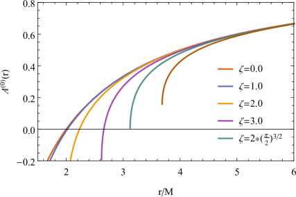
Figure 1: Plot of $A^{(0)}(r)$ as a function of $r$ (in units of $M$) for different values of $\zeta$ (in units of $M$). For $\zeta/M=0.0,1.0,2.0,3.0$ & $2\left(\frac{\pi}{2}\right)^{3/2}$, there exist event horizons, with $\zeta/M=2\left(\frac{\pi}{2}\right)^{3/2}$ representing the extremal case. However, for $\zeta=5.0$, no horizon exists.

Let us now consider the other function $\mu(r)=1-\frac{4M^{2}\zeta^{4}}{r^{6}}$ in the denominator of the $dr^{2}$-term of Eq. (1). As stated earlier, $\mu(r)$ at $r=r_{\text{min}}=(2M\zeta^{2})^{1/3}$ becomes null, and it approaches unity as $r\to\infty$. Moreover, if the conditions $\mu(r)=0$ and $A^{(0)}(r)\neq 0$ are simultaneously satisfied, then the metric component $g_{rr}$ will diverge, whereas $g_{tt}$ will remain finite. This particular situation resembles the throat of a wormhole. Therefore, we have two different kinds of radii – $r_{h}$ representing the position of an event horizon (satisfying the condition $A^{(0)}(r)=0$) and $r_{0}=r_{\text{min}}=(2M\zeta^{2})^{1/3}$ corresponding to the location of a possible wormhole throat (satisfying the condition $\mu(r)=0$). For the extremal case, both $A^{(0)}(r_{h})=0$ and $\mu(r_{0})=0$ are simultaneously satisfied yielding $r_{h}=r_{0}=M\pi$. A combined plot of $r_{h}$ and $r_{0}$ (in units of $M$) versus $\zeta$ (in units $M$) is shown in Fig.(2), for convenience.

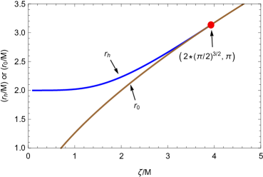
Figure 2: Combined plot of $r_{h}$ and $r_{0}$ (in units of $M$) versus $\zeta$ (in units $M$). It can be seen that $r_{h}>r_{0}$ for $\zeta/M<2\left(\frac{\pi}{2}\right)^{3/2}$ representing a black hole. The extremal case is denoted by the red dot having coordinates $\left(2\left(\frac{\pi}{2}\right)^{3/2},\pi\right)$. Beyond this point, $r_{h}$ does not exist signifying a wormhole spacetime with $r_{0}$ being the throat.

From this plot, it can be seen that $r_{h}>r_{0}$ for $\zeta/M<2\left(\frac{\pi}{2}\right)^{3/2}$, i.e., the event horizon is located outside the minimum radius or throat $r_{0}$ representing a black hole. The extremal case is denoted in the figure by the red dot having coordinates $\left(2\left(\frac{\pi}{2}\right)^{3/2},\pi\right)$. Beyond this point, $r_{h}$ does not exist, which signifies that the spacetime no longer represents a black hole when $\zeta/M>2\left(\frac{\pi}{2}\right)^{3/2}$. The Penrose diagrams for all the three cases viz. $\zeta/M>2\left(\frac{\pi}{2}\right)^{3/2}$, $\zeta/M=2\left(\frac{\pi}{2}\right)^{3/2}$ and $\zeta/M<2\left(\frac{\pi}{2}\right)^{3/2}$ have been shown in Figs. (1), (2) and (3) respectively in [22]. From the Penrose diagrams, it can be seen that the spacetime does represent a wormhole with $r_{0}$ being the throat for $\zeta/M>2\left(\frac{\pi}{2}\right)^{3/2}$ where $r_{h}$ cease to exist. To elaborate more on this aspect, let us consider the line element of a general static, spherically-symmetric wormhole of Morris-Thorne class as [79]

$$ds^{2}=-e^{2\Phi(r)}dt^{2}+\frac{dr^{2}}{1-\frac{\mathcal{B}(r)}{r}}+r^{2}\left(d\theta^{2}+\sin^{2}\theta d\phi^{2}\right)$$ (4)

where $\Phi(r)$ is called the red-shift function and $\mathcal{B}(r)$ is known as the shape function. The wormhole throat ($r_{0}$) establishes the connection between two different regions and satisfies the condition $\left(1-\frac{\mathcal{B}(r)}{r}\right)|_{r_{0}}=0$, i.e., $\mathcal{B}(r_{0})=r_{0}$. Additionally, $\mathcal{B}(r)$ satisfies the flare-out condition $\mathcal{B}^{\prime}(r_{0})<1$ also [79]. Moreover, $\Phi(r)$ must remain finite throughout (from the throat to infinity). If we compare the above line element with the line element of Eq. (1) for $n=0$, we see that the function $\left(1-\frac{\mathcal{B}(r)}{r}\right)$ can be equated to the function $\mu(r)=1-\frac{4M^{2}\zeta^{4}}{r^{6}}$, as $\mu(r)|_{r_{0}}=0$. Therefore, we obtain $\mathcal{B}(r)=\frac{4M^{2}\zeta^{4}}{r^{5}}$, which implies that $\mathcal{B}^{\prime}(r_{0})=-5<1$. Hence, the flare-out condition is also satisfied for this spacetime. The other function in the denominator of the $g_{rr}$-term of Eq. (1) with $n=0$ is $A^{(0)}(r)$ which always remains finite from $r_{0}$ to infinity, making the $g_{tt}$-term also finite. Therefore, this spacetime satisfies all the required conditions of a wormhole for $\zeta/M>2\left(\frac{\pi}{2}\right)^{3/2}$.
To summarize, it has been found that the spacetime given by Eq. (1) admits either a black hole or a wormhole corresponding to three possible scenarios as given below.

• Case-1: $\zeta/M<2\left(\frac{\pi}{2}\right)^{3/2}$ $\implies$ $r_{h}>r_{0}$ $\to$ Black Hole

• Case-2: $\zeta/M=2\left(\frac{\pi}{2}\right)^{3/2}$ $\implies$ $r_{h}=r_{0}=M\pi$ $\to$ Extremal Black Hole or Wormhole

• Case-3: $\zeta/M>2\left(\frac{\pi}{2}\right)^{3/2}$ $\implies$ $r_{h}$ does not exist $\to$ Wormhole

III Structure of Null Geodesics

We now consider the geodesic motion of photons in this spacetime. The line element of Eq. (1) being spherically-symmetric, we can choose $\theta=\frac{\pi}{2}$ without any loss of generality. Therefore, the Lagrangian describing the motion of photon in this geometry can be written as

$$2\mathcal{L}=-A^{(n)}(r)\dot{t}^{2}+\frac{\dot{r}^{2}}{\mu(r)A^{(n)}(r)}+C(r)\dot{\phi}^{2}$$ (5)

where an ‘overdot’ represents a derivative with respect to the affine parameter along the geodesic. The above Lagrangian admits two constants of motion, namely

$$\frac{\partial\mathcal{L}}{\partial\dot{t}}=-A^{(n)}(r)\dot{t}=-E~,~\frac{\partial\mathcal{L}}{\partial\dot{\phi}}=C(r)\dot{\phi}=L,$$ (6)

where $E$ and $L$ represent the magnitudes of energy and angular momentum of a photon with respect to an asymptotic observer. From normalization of the four velocity vectors, $g_{\mu\nu}\dot{x}^{\mu}\dot{x}^{\nu}=0$, we obtain

$$\frac{\dot{r}^{2}}{\mu(r)}+V_{eff}(r)=E^{2},\hskip 14.22636ptV_{eff}(r)=L^{2}\frac{A^{(n)}(r)}{C(r)},$$ (7)

where $V_{eff}(r)$ is the effective potential corresponding to radial motion.
A light ray coming from a source at infinity may pass through a turning point at some radial distance $r_{\text{tp}}$ and then escapes to an asymptotically faraway observer. When the ray travels from infinity towards the turning point, $\dot{r}<0$, and when it moves away from the turning point, $\dot{r}>0$. Therefore, at the turning point, $\dot{r}|_{r_{\text{tp}}}=0$, or $V_{eff}(r_{\text{tp}})=E^{2}$. From this expression, we obtain a relation of the impact parameter $b$ $(=L/E)$ (which is a constant of motion) in terms of the turning point ($r_{\text{tp}}$) of light trajectory as, $b(r_{\text{tp}})=\sqrt{C(r_{\text{tp}})/A^{(n)}(r_{\text{tp}})}$.

In case of circular photon orbits, $\dot{r}=\ddot{r}=0$, which yield $V_{eff}=E^{2}$ and $dV_{eff}/dr=0$ respectively. The second condition implies that circular orbits correspond to the maxima or minima of the effective potential. In case of maxima ($d^{2}V_{eff}/dr^{2}<0$), the light rings are unstable which we generally call as photon spheres; and minima of the effective potential ($d^{2}V_{eff}/dr^{2}>0$) give rise to stable light rings, termed as anti-photon spheres [76]. Therefore, a photon sphere (or an anti-photon sphere) at $r=r_{m}$ corresponds to $V_{eff}|_{r_{m}}=E^{2}$ and $(dV_{eff}/dr)|_{r_{m}}=0$ which respectively result in

$$b_{m}=\sqrt{C(r_{m})/A^{(n)}(r_{m})}~~~~\text{and}~~~~\frac{C^{\prime}(r_{m})}{C(r_{m})}-\frac{A^{(n)^{\prime}}(r_{m})}{A^{(n)}(r_{m})}=0,$$ (8)

where a prime denotes derivative with respect to $r$ and $b_{m}(=b|_{r_{m}})$ is called as the critical impact parameter corresponding to a photon sphere.
Putting the expressions of $A^{(n)}(r)$ and $C(r)$ in the second expression of Eq. (8) and simplifying, we obtain the following equation for photon sphere,

$$r_{m}^{6}-9M^{2}r_{m}^{4}-4M^{2}\zeta^{4}=0.$$ (9)

Interestingly, it is found that the above photon sphere equation does not depend on the parameter $n$. It depends only on $\zeta$. Therefore, the radius of the photon sphere will depend on the quantum parameter $\zeta$ only, as given below

$$r_{m}=M\sqrt{3+9\eta^{-1/3}+\eta^{1/3}}~~~~\text{where}~~~~\eta=27+2\tilde{\zeta}^{4}+2\tilde{\zeta}^{2}\sqrt{27+\tilde{\zeta}^{4}}~~~\text{and}~~~\tilde{\zeta}=\zeta/M.$$ (10)

It can be easily verified from the above equation that $r_{m}=3M$ for $\zeta=0$, i.e., we recover the radius of the photon sphere in Schwarzschild spacetime. The critical impact parameter ($b_{m}$) due to the photon sphere is obtained from the first expression of Eq. (8) as given below

$$b_{m}=\left[\frac{1}{r_{m}^{2}}-\frac{n\pi}{\zeta^{2}}-\frac{(-1)^{n}}{\zeta^{2}}\arcsin\left(\frac{2M\zeta^{2}}{r_{m}^{3}}\right)\right]^{-1/2},$$ (11)

where $r_{m}$ is given by Eq. (10).
Plots of $V_{eff}/L^{2}$ as functions of (a) $r/M$ (Black hole) and (b) $l/M$ (Wormhole) with $n=0$ for different values of $\zeta$ (in units of $M$) are shown in Figs. (3(a)) and (3(b)) respectively. In Fig. (3(a)) for the black hole case, the radii of photon spheres increase with increasing value of $\zeta$. Since minimum of the effective potential does not exist, there will no anti-photon sphere, which is usually the case for black holes. On the other hand, in Fig. (3(b)) for the wormhole case, $V_{eff}$ is plotted against the proper radial coordinate $l$ which is defined as

$$l(r)=\pm\int_{r_{0}}^{r}\frac{dr}{1-\frac{\mathcal{B}(r)}{r}}=\pm\int_{r_{0}}^{r}\frac{dr}{1-\frac{4M^{2}\zeta^{4}}{r^{6}}}.$$ (12)

In terms of this, the wormhole throat is at $l(r_{0})=0$ and the two signs correspond to the two regions connected by the throat. In the present case, $1-\frac{\mathcal{B}(r)}{r}=\mu(r)=1-\frac{4M^{2}\zeta^{4}}{r^{6}}$, as discussed before.

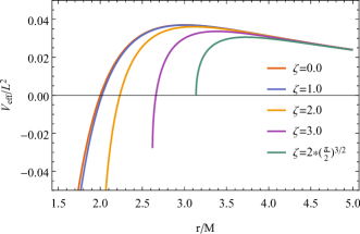
(a) Black hole

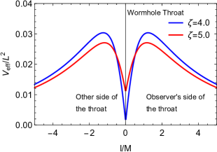
(b) Wormhole

Figure 3: Plots of $V_{eff}/L^{2}$ as functions of (a) $r/M$ (Black hole) and (b) $l/M$ (Wormhole) with $n=0$ for different values of $\zeta$. The maxima of $V_{eff}$ correspond to the locations of photon spheres. In figure (a) for the black hole case, the radii of photon spheres increase with increasing value of $\zeta$. In figure (b) for the wormhole case, $V_{eff}$ is plotted against the proper radial coordinate $l$, such that at the throat $l(r_{0})=0$.

IV Constraints on $\zeta$ from Observations

In this section, bounds on the quantum parameter $\zeta$ are provided for $n=0$ based on the observational results by the EHT Collaboration of shadows of the central objects of the M87* and SgrA* galaxies. A recent study on the shadows and light rings for this spacetime can be found in [36]. A discussion on the possible bounds on $\zeta$ are also provided there. However, since this aspect is crucial for the rest of our discussion, we shall briefly elaborate upon it for completeness.
Radius of the shadow with respect to the observer’s sky (which is equivalent to the corresponding critical impact parameter) for $n=0$ is evaluated from Eq. (11) as

$$R_{\text{sh}}=b_{m}=\left[\frac{1}{r_{m}^{2}}-\frac{1}{\zeta^{2}}\arcsin\left(\frac{2M\zeta^{2}}{r_{m}^{3}}\right)\right]^{-1/2}.$$ (13)

Recent observation by the EHT Collaboration for M87* galaxy provide a mass of $M=(6.5\pm 0.7)\times 10^{9}M_{\odot}$, a distance of $D=(16.8\pm 0.8)$ Mpc from the observer and the angular diameter of the shadow to be $\Delta\theta_{\text{sh}}=42\pm 3$ $\mu$as [38], where $\Delta\theta_{\text{sh}}=2R_{\text{sh}}/D$. The observed value of the shadow diameter $d_{\text{sh}}(=2R_{\text{sh}})$, in dimensionless unit, is found to be [38]

$$\frac{d_{\text{sh}}}{M}=11.0\pm 1.5.$$ (14)

Therefore, from the M87* observation, we obtain the following range of $R_{\text{sh}}$:

$$4.75M\leq R_{\text{sh}}\leq 6.25M.$$ (15)

On the other hand, observations on the SgrA* have reported a fractional deviation parameter $\delta$, which measures the fractional deviation of the observed shadow diameter from that of the Schwarzschild one, given by

$$\delta=\frac{d_{\text{sh}}}{d_{\text{sh,Sch}}}-1=\frac{R_{\text{sh}}}{R_{\text{sh,Sch}}}-1=\frac{R_{\text{sh}}}{3\sqrt{3}M}-1\implies R_{\text{sh}}=3\sqrt{3}(\delta+1)M$$ (16)

The EHT collaboration has provided two sets of values of $\delta$ from the Keck and the Very Large Telescope Interferometer (VLTI) observations, as given below [41, 42, 43]

$$\delta=\begin{cases}-0.04^{+0.09}_{-0.10}&\text{(Keck)}\\ -0.08^{+0.09}_{-0.09}&\text{(VLTI)}.\end{cases}$$ (17)

Therefore, the values of $\delta$ lie in the range $-0.14\leq\delta\leq+0.05$ (Keck) and $-0.17\leq\delta\leq+0.01$ (VLTI). From Eq. (16), the corresponding ranges of the shadow radius of SgrA* can be evaluated as,

$$4.47M\leq R_{\text{sh}}\leq 5.46M~~~\text{(Keck)}~~~~~\text{and}~~~~~4.31M\leq R_{\text{sh}}\leq 5.25M~~~\text{(VLTI)}.$$ (18)

Plots of $R_{\text{sh}}$ (units of $M$) as functions of $\zeta$ (in units of $M$), along with allowed ranges from observations, are shown in Fig. (4(a)) for SgrA* and in Fig. (4(b)) for M87*.

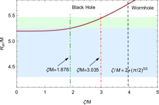
(a) SgrA*

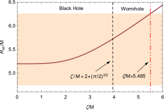
(b) M87*

Figure 4: Plots of $R_{\text{sh}}$ (in units of $M$) as a function of $\zeta$ (in units of $M$). The shaded regions represent the observational ranges of $R_{\text{sh}}/M$ for (a) SgrA* and (b) M87*. The values of $\zeta/M$ that fall within these shaded regions should be allowed. In (a), the ‘light blue’ shaded region represents VLTI and ‘light green’ region corresponds to Keck observations. Constraints on $\zeta$ have been shown with vertical lines: green dot-dashed for VLTI and red dot-dashed for Keck. In (b), the ‘light orange’ shaded region represents M87* observational range. Constraints on $\zeta$ have been shown with vertical red dot-dashed line. The black-dashed vertical lines in both the plots correspond to the extremal value of $\zeta$.

The shaded regions in both the plots represent the observational ranges of $R_{\text{sh}}/M$. The deep brown curve represents the variation of $R_{\text{sh}}/M$ as a function of $\zeta/M$. The black-dashed vertical line in both the plots in Fig. (4) correspond to $\zeta/M=2\left(\frac{\pi}{2}\right)^{3/2}\approx 3.937$. The left side of this line ,i.e., $\zeta/M<2\left(\frac{\pi}{2}\right)^{3/2}$ represents the black hole and the right side of it stands for the wormhole. In case of M87* observations, it can be seen from Fig. (4(b)) that the maximum allowed value of $\zeta$ is $5.485M$ (denoted by the red dot-dashed vertical line). So the observational constraint on $\zeta$ from M87* observations turns out be $\zeta/M\in[0,5.485]$. Therefore, both the black hole and the wormhole cases are allowed in this scenario.
On the other hand, in case of SgrA* observations shown in Fig. (4(a)), the ‘light blue’ shaded region represents the observational range of $\zeta/M$ for VLTI and ‘light green’ shaded region corresponds to the Keck observation. In case of VLTI, the maximum allowed value of $\zeta$ is found out to be $1.878M$ (denoted by the green dot-dashed vertical line) and in case of Keck, it is $3.035M$ (denoted by the red dot-dashed vertical line). So, the observational constraints form SgrA* results come out to be $\zeta/M\in[0,1.878]$ for VLTI and $\zeta/M\in[0,3.035]$ for Keck. Since both the maximum allowed values of $\zeta$ are less than $2M\left(\frac{\pi}{2}\right)^{3/2}\approx 3.937M$, they fall within the black hole case only. Hence, M87* observations support both black hole and wormhole cases; whereas SgrA* observations put more stringent constraints supporting black hole case only. We shall now explore the strong lensing features of this spacetime considering both black hole and wormhole cases in the following sections.

V Lensing of Light in the Strong Deflection Limit

To study the strong lensing of light, let us consider a general static, spherically symmetric spacetime represented by the following line element

$$ds^{2}=-F(r)dt^{2}+G(r)dr^{2}+C(r)\left(d\theta^{2}+\sin^{2}\theta d\phi^{2}\right).$$ (19)

A ray of light having impact parameter $b>b_{m}$, where $b_{m}$ refers to the critical impact parameter corresponding to a photon sphere, starts from a distant source, moves towards the central lensing object, takes a turn at $r_{\text{tp}}$ (where $\dot{r}|_{r_{\text{tp}}}=0$) and finally escapes to a distant observer. The bending angle $\alpha(r_{\text{tp}})$ for such a light ray can be obtained as [47, 52]

$$\alpha(r_{\text{tp}})=I(r_{\text{tp}})-\pi,$$ (20)

where

$$I(r_{\text{tp}})=2\int^{\infty}_{r_{\text{tp}}}\frac{dr}{\sqrt{\frac{R(r)C(r)}{G(r)}}}~,~R(r)=\left(\frac{F(r_{\text{tp}})C(r)}{F(r)C(r_{\text{tp}})}-1\right).$$ (21)

Again, it has been discussed earlier that the impact parameter ($b$) for such a ray having a turning point at $r_{\text{tp}}$ is given as, $b(r_{\text{tp}})=\sqrt{C(r_{\text{tp}})/F(r_{\text{tp}})}$. Eliminating $r_{\text{tp}}$ from $\alpha(r_{\text{tp}})$ and $b(r_{\text{tp}})$, the bending angle can be expressed as a function of the impact parameter, i.e., $\alpha(b)$. In a spacetime having photon sphere ($r_{m}$) only, the bending angle diverges logarithmically as $r_{\text{tp}}\to r_{m}$ or $b\to b_{m}$ when the light ray approaches the photon sphere from $b>b_{m}$ side. A comprehensive study of strong lensing due to a photon sphere can be found in [47, 52]. The corresponding divergence of bending angle due to photon sphere (for both black holes and wormholes) in the strong deflection limit, i.e., $r_{\text{tp}}\to r_{m}$ or $b\to b_{m}$, is given as [52]

$$\alpha(b)=-\bar{a}\log\left(\frac{b}{b_{m}}-1\right)+\bar{b}+\mathcal{O}((b-b_{m})\log(b-b_{m})),$$ (22)

where $\bar{a}$ and $\bar{b}$ are given by

$$\bar{a}=\sqrt{\frac{2G(r)F(r)}{C^{{}^{\prime\prime}}(r)F(r)-C(r)F^{{}^{\prime\prime}}(r)}}\Biggr{\rvert}_{r_{m}}~,~\bar{b}=\bar{a}\log\left[r^{2}\left(\frac{C^{{}^{\prime\prime}}(r)}{C(r)}-\frac{F^{{}^{\prime\prime}}(r)}{F(r)}\right)\right]\Biggr{\rvert}_{r_{m}}+I_{R}(r_{m})-\pi.$$ (23)

Here, prime denotes a derivative with respect to $r$, and $I_{R}(r_{m})$ is a constant [52]. Plots of $\bar{a}$ and $\bar{b}$ as functions of $\zeta/M$ for $n=0$ are shown in Figs. (5(a)) and (5(b)) respectively. Markers are provided with vertical lines for $\zeta=1.878M$ (VLTI), $\zeta=3.035M$ (Keck), $\zeta=2\left(\frac{\pi}{2}\right)^{3/2}M$ and $\zeta=5.485M$ (M87*).

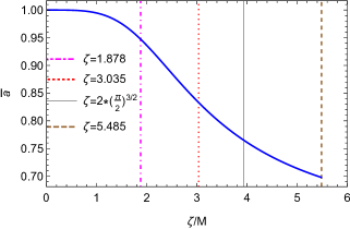
(a) Variation of $\bar{a}$ with $\zeta/M$

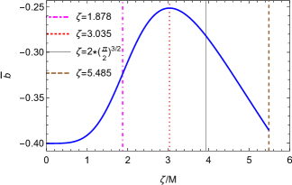
(b) Variation of $\bar{b}$ with $\zeta/M$

Figure 5: Plots of (a) $\bar{a}$ and (b) $\bar{b}$ as functions of $\zeta$ (in units of $M$) for $n=0$. Markers are provided with vertical lines for $\zeta=1.878M$ (VLTI), $\zeta=3.035M$ (Keck), $\zeta=2\left(\frac{\pi}{2}\right)^{3/2}M$ and $\zeta=5.485M$ (M87*).

The specific values of $\bar{a}$ and $\bar{b}$ are also provided in Table (1) for the above set of values of $\zeta$.

Table 1: Values of $\bar{a}$ and $\bar{b}$ for different values of $\zeta$ (in units of $M$). The second column is for $\zeta=0.0$ corresponding to the Schwarzschild black hole. The third and fourth columns are for $\zeta=1.878M$ and $\zeta=3.035M$ respectively, which represent the maximum allowable values of $\zeta$ constrained from the VLTI and Kcck observations of SgrA* respectively. The fifth column corresponds to the extremal black hole for $\zeta=2\left(\frac{\pi}{2}\right)^{3/2}M$. And the last column stands for $\zeta=5.485M$ which represents the maximum allowable value of $\zeta$ from M87* observation. The last column represents the wormhole case, and rest of the others represent black hole cases. Numerical values are obtained in natural units.

	$\zeta=0$	$~\zeta=1.878M~$	$~\zeta=3.035M~$	$~\zeta=2\left(\frac{\pi}{2}\right)^{3/2}M~$	$~\zeta=5.485M~$
	(Schwarzschild)	(VLTI)	(Keck)	(Extremal)	(M87*)
$~\bar{a}~$	1	0.9473	0.8330	0.7649	0.6979
$~\bar{b}~$	-0.40023	-0.3238	-0.2514	-0.2822	-0.3856

Plots of bending angle ($\alpha$) versus impact parameter ($b$) (in units of $M$) are shown in Fig. (6) for the set of values of $\zeta$ as considered in Table (1), i.e., $\zeta=\{0.0,~1.878M,~3.035M,~2\left(\frac{\pi}{2}\right)^{3/2}M,~5.485M\}$. Here, plots are obtained from the exact expression of $\alpha$ using Eqs. (20) and (21). It can be seen from the figure that the Schwarzschild and VLTI plots almost merge with each other. So, if $\zeta$ is constrained according to the VLTI observation, it will be difficult to distinguish this black hole from the Schwarzschild one, making it a candidate for Schwarzschild black hole mimicker. With increase of $\zeta$, the deviations from the Schwarzschild black hole become larger for the Keck and extremal black hole cases. On the other hand, if $\zeta$ is constrained according to the M87* observations, the deviations for the wormhole cases are found out to be significant from the Schwarzschild black hole.

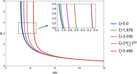
Figure 6: Plots of bending angle ($\alpha$) versus impact parameter ($b$) (in units of $M$) for $\zeta=\{0.0,~1.878M,~3.035M,~2\left(\frac{\pi}{2}\right)^{3/2}M,~5.485M\}$.

VI Strong Lensing Observables

In this section, we shall discuss about various observables corresponding to the relativistic images formed due to photon sphere in the context of strong gravitational lensing of the quantum gravity spacetime under consideration. Expressions of most of these observables for the relativistic images formed just outside the photon sphere have been obtained in Ref. [47]. The lens equation in the strong deflection limit, considering the source, lensing object and observer to be nearly aligned (thin lens approximation), is given as [46]

$$\delta=\theta-\frac{D_{LS}}{D_{OS}}\Delta\alpha_{n},$$ (24)

where $\delta$ is the angular separation between the light source and the lensing object, $\theta$ is the angular separation between the image and the lensing object, $D_{LS}$ is the distance between the lensing object and the light source, $D_{OS}$ is the distance between the observer and the light source. Since light rays take a number of turns (say, $n$) before reaching the observer in the strong field limit, the corresponding offset of deflection angle is represented by $\Delta\alpha_{n}=\alpha(\theta)-2\pi n$. Note that $D_{OS}=D_{OL}+D_{LS}$, where $D_{OL}$ is the distance between the observer and the lensing object.

The angular position of $n$-th relativistic image formed just outside the photon sphere can be approximated by [46, 47]

$$\theta_{n}\approx\theta_{n}^{0}+\frac{b_{m}e_{n}(\delta-\theta_{n}^{0})D_{OS}}{\bar{a}D_{LS}D_{OL}},\quad e_{n}=e^{\frac{\bar{b}-2n\pi}{\bar{a}}},$$ (25)

where $\theta_{n}^{0}=\frac{b_{m}}{D_{OL}}(1+e_{n})$ is the image position corresponding to $\alpha\left(\theta_{n}^{0}\right)=2n\pi$. It is to be noted that the second term in the above equation is negligible as compared to $\theta_{n}^{0}$. Therefore, for practical purposes, we can roughly take

$$\theta_{n}=\theta_{n}^{0}=\frac{b_{m}}{D_{OL}}(1+e_{n})=\theta_{\infty}(1+e_{n}),$$ (26)

where $\theta_{\infty}=b_{m}/D_{OL}$ is the angular position of the relativistic image formed at the photon sphere. Moreover, the magnification of the $n$-th relativistic image is given as [47]

$$\mu_{n}=\left(\frac{\delta}{\theta}\frac{\partial\delta}{\partial\theta}\right)^{-1}\bigg{\rvert}_{\theta^{0}_{n}}=\frac{b_{m}^{2}e_{n}(1+e_{n})D_{OS}}{\bar{a}\delta D_{OL}^{2}D_{LS}}.$$ (27)

It should be noted that $\theta_{1}$ corresponding to $n=1$ represents the angular position of the outermost relativistic image just outside the photon sphere, and $\theta_{\infty}$ corresponds to the innermost one at the photon sphere. This implies that the angular positions of the relativistic images decrease with increasing $n$. It is usually observed that the inner images are closely packed together with the innermost one; leaving only the first (outermost) one ($n=1$) to be resolved from the rest. Therefore, two more lensing observables can be defined, namely $s_{1}$ representing the angular separation between first and the rest (effectively the innermost one), and $r_{1}$ denoting the relative magnification of the outermost image, defined by the ratio of the magnification of the first image and the sum of magnifications of the rest. They are given by [47]

$$s_{1}=\theta_{1}-\theta_{\infty}=\theta_{\infty}e_{1},$$ (28)

$$r_{1}=\frac{\mu_{1}}{\sum\limits_{m=2}^{\infty}\mu_{m}}\approx e^{\frac{2\pi}{\bar{a}}}.$$ (29)

Moreover, since light rays forming relativistic images in the strong deflection limit may take turn around the lensing object multiple times before coming to the observer, travel time of photons through different light paths may be significantly different for different relativistic images. The difference of travel time for different images may produce detectable effects, giving rise to another important lensing observable, namely Time Delay. Substantive discussion on this observable can be found in Ref. ([80]). In case of a general static, spherically symmetric spacetime represented by the line element in Eq. (19), the time delay ($\Delta T$) between $n$-th and $m$-th relativistic images is given as [80]

$$\Delta T^{s}_{n,m}=2\pi(n-m)b_{m}+2\sqrt{\frac{G_{m}}{F_{m}}}\sqrt{\frac{b_{m}}{p}}~e^{\frac{\bar{b}}{2\bar{a}}}\left(e^{-\frac{2m\pi\mp\delta}{2\bar{a}}}-e^{-\frac{2n\pi\mp\delta}{2\bar{a}}}\right),$$ (30)

when the two images are on the same side of the optic axis (line joining lens and observer) with the upper negative sign before $\delta$ signifying both the images and the source (all three together) on the same side of the optic axis, and the lower positive sign before $\delta$ signifying both the images together on the same side of the optic axis and the source on the opposite side of the optic axis, whereas

$$\Delta T^{o}_{n,m}=[2\pi(n-m)-2\delta]b_{m}+2\sqrt{\frac{G_{m}}{F_{m}}}\sqrt{\frac{b_{m}}{p}}~e^{\frac{\bar{b}}{2\bar{a}}}\left(e^{-\frac{2m\pi-\delta}{2\bar{a}}}-e^{-\frac{2n\pi+\delta}{2\bar{a}}}\right),$$ (31)

when the two images are on the opposite side of the optic axis, i.e., one of the image and the source are on one side together and the other image is on the opposite side of the optic axis. Here, $p=\frac{C_{m}^{\prime\prime}F_{m}-C_{m}F_{m}^{\prime\prime}}{4\sqrt{F_{m}^{3}C_{m}}}$. When the source is almost aligned with the optic axis ($\delta\ll 2\pi$), it can be shown that $\Delta T^{o}_{n,n}\ll\Delta T^{s}_{n,m\neq n}\approx\Delta T^{o}_{n,m\neq n}$ [80]. Moreover, the second terms on the RHS of the above equations are much smaller than the first terms ($\sim 1\%$ contribution). Therefore, considering thin lens approximation, the expression for $\Delta T$ considered for the present analysis is

$$\Delta T_{n,m}=2\pi(n-m)b_{m}=2\pi(n-m)\theta_{\infty}D_{OL},\quad[m\neq n].$$ (32)

Upon describing the necessary formalism, we are now in a position to analyze the observables in the context of the effective gravity spacetime under consideration, considering both the SgrA* and M87* observations. For the present analysis, we have restored $G$ and $c$ to replace $M$ by $\frac{GM}{c^{2}}$ where in the last expression $M$ represents the actual mass obtained from observation. The observer-lens distance ($M_{OL}$) has also been taken from observational data. Moreover, we have set $M_{LS}=M_{OL}=\frac{1}{2}M_{OS}$.
In case of SgrA*, the values we have considered are, $M=4.0\times 10^{6}M_{\odot}$ and $D_{OL}=8.35$ Kpc [41, 42, 43]. Whereas, for M87*, the corresponding values are, $M=6.5\times 10^{9}M_{\odot}$ and $D_{OL}=16.8$ Mpc [38]. In addition, we have considered $\delta=5^{\circ}$ for all the computations. The results have been depicted through figures and tabular forms, considering both SgrA* and M87* observations.

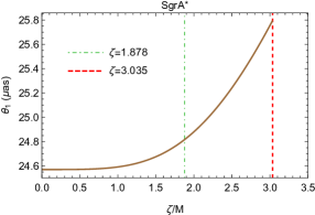
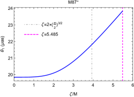
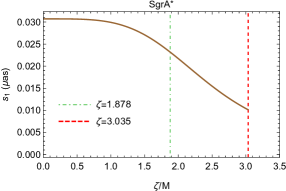
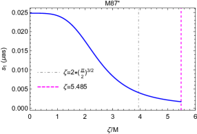
Figure 7: Plots of $\theta_{1}$ (top panel) and $s_{1}$ (bottom panel) as functions of $\zeta/M$. All angles are in ‘micro-arcsecond’. The left panel corresponds to SgrA* and the right panel represents M87* observations. In left panel, markers with vertical lines are provided signifying VLTI (green, dot-dashed line at $\zeta=1.878M$) and Keck (red, dashed line at $\zeta=3.035M$) observations. In right panel, black dot-dashed vertical line at $\zeta=2\left(\frac{\pi}{2}\right)^{3/2}M$ represents the transition between black hole and wormhole cases, and the magenta dashed line at $\zeta=5.485M$ stands for the maximum allowed limit of $\zeta$ for wormhole case from M87* observation.

In Fig. (7), the angular position ($\theta_{1}$) of the first (outermost) image just outside the photon sphere (top panel) and the separation ($s_{1}=\theta_{1}-\theta_{\infty}$) of it from the innermost image at the photon sphere (bottom panel) are plotted as functions of $\zeta/M$. The left panel corresponds to the SgrA* and the right panel represents the M87* observations. It can be seen from the plots that $\theta_{1}$ rises with increasing values of $\zeta$, but $s_{1}$ decreases. This clearly signifies that it will become increasingly difficult to resolve the first image from the rest with higher values of $\zeta$. Importantly, relativistic images for the wormhole (region in the right side of the black-dashed vertical line in the right panel of M87*) turn out to be more difficult to resolve than the black hole counterpart.

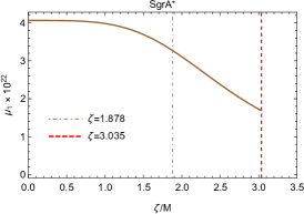
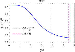
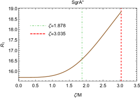
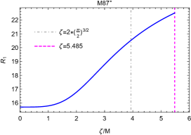
Figure 8: Plots of $\mu_{1}$ (top panel) and $\mathcal{R}_{1}$ (bottom panel) as functions of $\zeta/M$. The left panel corresponds to SgrA* and the right panel represents M87* observations. The markers with vertical lines carry the same meaning as described in the caption of Fig. (7).

Similarly, in Fig. (8), the absolute magnification $\mu_{1}$ and the relative flux, converted to magnitude using $\mathcal{R}_{1}=2.5\log r_{1}$, of the first (outermost) image are plotted against $\zeta/M$. It can be seen that the images get increasingly de-magnified with increase of $\zeta$, but $\mathcal{R}_{1}$ increases. Here also, relativistic images for wormhole will have much lower magnification as compared to black hole.

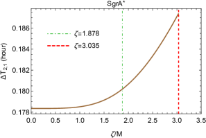
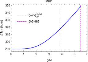
Figure 9: Plots of time delay $\Delta T_{2,1}$ (in hour) as functions of $\zeta/M$. The left panel corresponds to SgrA* and the right panel represents M87* observations. The markers with vertical lines carry the same meaning as described in the caption of Fig. (7).

In Fig. (9), the time delay between the first and second relativistic images ($\Delta T_{2,1}$) is plotted against $\zeta/M$. It is evident from the figure that the time delay comes out to be of the orders of minutes for SgrA* and around several days for M87*. Such short time delays in SgrA* provide little chance of observation, whereas it yields measurable time delay in case of M87* observation. While most of the other observables provide negligible opportunity for detection and distinction between black hole and wormhole cases, time delay may become crucial in this aspect, at least for ultra compact objects having masses of the order of M87*. Specific values of these lensing observables have also been presented in Table (2) for convenience.

Table 2: Specific values of lensing observables for both SgrA* and M87*. All angles are in ‘micro-arcsecond’ and $r_{n}$ is converted to magnitude using $\mathcal{R}_{n}=2.5\log r_{n}$. Here, we have considered $M=4.0\times 10^{6}M_{\odot}$, $D_{OL}=D_{LS}=8.35$ Kpc for SgrA* and $M=6.5\times 10^{9}M_{\odot}$, $D_{OL}=D_{LS}=16.8$ Mpc for M87*, and $\delta=5^{\circ}$ for both. The second, third and fourth columns correspond to the SgrA* black hole cases and the last column represents the M87* wormhole case. Since the extremal case (fifth column) falls outside the domain of SgrA* observation, its values are obtained using the M87* data.

	$\zeta=0$	$\zeta=1.878M$	$\zeta=3.035M$	$\zeta=2\left(\frac{\pi}{2}\right)^{3/2}M$	$\zeta=5.485M$
	(Schwarzschild)	(VLTI)	(Keck)	(Extremal)	(M87*)
$\theta_{1}$ ($\mu$as)	24.5701	24.8167	25.7955	21.8191	23.8410
$\theta_{\infty}$ ($\mu$as)	24.5394	24.7935	25.7854	21.8150	23.8393
$s_{1}$ ($\mu$as)	0.0307	0.0232	0.0101	0.0041	0.0017
$\mu_{1}\times 10^{22}$	4.0647	3.2725	1.6861	0.6276	0.3105
$\mathcal{R}_{1}$	15.7064	16.5811	18.8558	20.5355	22.5085
$\Delta T_{2,1}$ (hour)	0.1784	0.1802	0.1874	319.001	348.602

VII Conclusion

In this work, we study gravitational lensing in the strong deflection limit by the third type of EQG solution proposed in Ref. ([23]). The line element of the spacetime depends on two free parameters $n$ and $\zeta$. Our whole calculation is performed for $n=0$. It has been found that the spacetime is asymptotically flat for any finite value of $\zeta$ and reduces to the Schwarzschild black hole in the limit $\zeta\to 0$. So, $\zeta$ acts as the modified quantum parameter of the theory for $n=0$. For a specific range of values of $\zeta\in[0,2\left(\frac{\pi}{2}\right)^{3/2}]$ (in units of $M$), the spacetime contains event horizon. Whereas beyond this range, there exists a minimum value of the radial coordinate which is shown to act like a wormhole throat. Hence, the spacetime contains both black hole and wormhole solutions with $\zeta=2\left(\frac{\pi}{2}\right)^{3/2}M\approx$ being the transition or extremal case. Using EHT data from SgrA* and M87* observations, the allowable ranges of $\zeta$ are obtained as $\zeta\in[0,1.878M]$ (VLTI), $\zeta\in[0,3.035M]$ (Keck), and $\zeta\in[0,5.485M]$ (M87*). It signifies that the wormhole case is ruled out by SgrA* observations, while both black hole and wormhole cases are possible by M87* observations.

We, then, obtain the deflection angle parameters in the strong field regime following [47, 52], generated their plots as functions of $\zeta$ and compared them with the Schwarzschild case. In addition, we analyze the strong lensing observables and described the effects of the quantum parameter $\zeta$ on them through their representative plots. It is found that, with increase of $\zeta$, it becomes difficult to resolve and detect the relativistic images outside the photon sphere. However, time delay between the first two relativistic images comes out to be of the order of several days in case of M87* observation, which may have the potential for detection in future observations.

To conclude, our theoretical study suggests that the quantum parameter plays an important role in the strong lensing characteristics and observables.The present analysis are also important in the sense that it opens up multiple exciting research prospects such as studying the strong lensing features of this spacetime when $n\neq 0$, analyzing the physics of accretion disks in this background and generating its image etc. We intend to envisage them in future.

References

- [1] A. Einstein, “Die Grundlage der allgemeinen Relativitatstheorie”, Ann. Phys. 49 (1916) 769–822.
- [2] R. Penrose, “Gravitational collapse and space-time singularities”, Phys. Rev. Lett. 14, 57 (1965).
- [3] S. W. Hawking and G. F. Ellis, “The large scale structure of space-time”, Cambridge University Press, 2023.
- [4] A. Ashtekar, B. K. Berger, J. Isenberg, and M. MacCallum, “General Relativity and Gravitation: A Centennial Perspective”, Cambridge University Press, 2015.
- [5] T. Clifton, P. G. Ferreira, A. Padilla, and C. Skordis, “Modified gravity and cosmology”, Physics Reports 513, 1 (2012); arXiv:1106.2476 [astro-ph.CO].
- [6] S. Mukohyama and K. Noui, “Minimally modified gravity: a Hamiltonian construction”, JCAP 07, 049 (2019), arXiv:1905.02000 [gr-qc].
- [7] C. Rovelli, “Quantum gravity”, Cambridge Monographs on Mathematical Physics, Cambridge University Press, 2004.
- [8] T. Thiemann, “Modern Canonical Quantum General Relativity”, Cambridge Monographs on Mathematical Physics, Cambridge University Press, 2007.
- [9] H. Maeda, “Quest for realistic non-singular black-hole geometries: regular-center type”, JHEP 11 (2022), 108; arXiv:2107.04791 [gr-qc].
- [10] C. Lan, H. Yang, Y. Guo and Y. G. Miao, “Regular black holes: A short topic review”, Int J Theor Phys 62, 202 (2023); arXiv:2303.11696 [gr-qc].
- [11] P. Nicolini, A. Smailagic, and E. Spallucci, “Noncommutative geometry inspired Schwarzschild black hole”, Phys. Lett. B 632, 547 (2006); arXiv:grqc/0510112.
- [12] F. Nasseri, “Schwarzschild black hole in noncommutative spaces”, Gen. Rel. and Grav. 37, 2223 (2005); arXiv:hep-th/0508051.
- [13] J. F. Donoghue, “General relativity as an effective field theory: The leading quantum corrections”, Phys. Rev. D 50, 3874 (1994); arXiv:gr-qc/9405057.
- [14] C. P. Burgess, “Quantum Gravity in Everyday Life: General Relativity as an Effective Field Theory”, Living Rev. Rel. 7, 5 (2004); arXiv:gr-qc/0311082.
- [15] A. Ashtekar and E. Bianchi, “A Short Review of Loop Quantum Gravity”, Rept. Prog. Phys. 84, 042001 (2021); arXiv:2104.04394 [gr-qc].
- [16] A. Perez, “Black Holes in Loop Quantum Gravity”, Rept. Prog. Phys. 80, 126901 (2017); arXiv:1703.09149 [gr-qc].
- [17] M. Bojowald, “Absence of Singularity in Loop Quantum Cosmology”, Phys. Rev. Lett. 86, 5227 (2001); arXiv:gr-qc/0102069.
- [18] C. G. Bohmer and K. Vandersloot, “Loop quantum dynamics of the Schwarzschild interior”, Phys. Rev. D 76, 104030 (2007); arXiv:0709.2129 [gr-qc].
- [19] D. W. Chiou, “Phenomenological loop quantum geometry of the Schwarzschild black hole”, Phys. Rev. D 78, 064040 (2008); arXiv:0807.0665 [gr-qc].
- [20] S. Saini and P. Singh, “Generic absence of strong singularities in loop quantum Bianchi-IX spacetimes”, Class. Quant. Grav. 35, 065014 (2018); arXiv:1712.09474 [gr-qc].
- [21] N. Bodendorfer, F. M. Mele, and J. Munch, “Effective Quantum Extended Spacetime of Polymer Schwarzschild Black Hole”, Class. Quant. Grav. 36, 195015 (2019); arXiv:1902.04542 [gr-qc].
- [22] C. Zhang, J. Lewandowski, Y. Ma and J. Yang, “Black Holes and Covariance in Effective Quantum Gravity,” arXiv:2407.10168 [gr-qc].
- [23] C. Zhang, J. Lewandowski, Y. Ma and J. Yang, “Black Holes and Covariance in Effective Quantum Gravity: A solution without Cauchy horizons,” arXiv:2412.02487 [gr-qc].
- [24] R.A. Konoplya and O.S. Stashko, “Probing the Effective Quantum Gravity via Quasinormal Modes and Shadows of Black Holes”, arXiv:2408.02578.
- [25] Z. Malik, “Perturbations and Quasinormal Modes of the Dirac Field in Effective Quantum Gravity”, arXiv:2409.01561.
- [26] H. Liu, M.Y. Lai, X.Y. Pan, H. Huang and D.C. Zou, “Gravitational lensing effect of black holes in effective quantum gravity”, Phys. Rev. D 110, 104039 (2024); arXiv:2408.11603 [gr-qc].
- [27] Y. Wang, A. Vachher, Q. Wu, T. Zhu and S. G. Ghosh, “Strong Gravitational Lensing by Static Black Holes in Effective Quantum Gravity”, arXiv:2410.12382.
- [28] W. Liu, D. Wu and J. Wang, “Light rings and shadows of static black holes in effective quantum gravity”, Phys. Lett. B 858, 139052 (2024); arXiv:2408.05569 [gr-qc].
- [29] Y.H. Shu and J.H. Huang, “Circular orbits and thin accretion disk around a quantum corrected black hole”, arXiv:2412.05670.
- [30] J. Lin, X. Zhang and M. Bravo-Gaete, “Mass inflation and strong cosmic censorship conjecture in covariant quantum gravity black hole”, arXiv:2412.01448.
- [31] Z. Ban, J. Chen and J. Yang, “Shadows of rotating black holes in effective quantum gravity”, arXiv:2411.09374.
- [32] G.P. Li, H.B. Zheng, K.J. He and Q.Q. Jiang, “The shadow and observational images of the non-singular rotating black holes in loop quantum gravity”, arXiv:2410.17295.
- [33] A. Vachher, S.G. Ghosh, “Strong Gravitational Lensing by Rotating Quantum-Corrected Black Holes: Insights and Constraints from EHT Observations of M87* and SgrA*”, arxiv:2410.11332 [gr-qc].
- [34] M. Azreg-Aınou, “From static to rotating to conformal static solutions: Rotating imperfect fluid wormholes with(out) electric or magnetic field”, Eur. Phys. J. C 74, 2865 (2014); arXiv:1401.4292 [gr-qc].
- [35] M. Azreg-Aınou, “Generating rotating regular black hole solutions without complexification”, Phys. Rev. D 90, 064041 (2014); arXiv:1405.2569 [gr-qc].
- [36] W. Liu, D. Wu and J. Wang, “Light rings and shadows of static black holes in effective quantum gravity II: A new solution without Cauchy horizons”, arXiv:2412.18083 [gr-qc].
- [37] F.W. Dyson, A. S. Eddington, and C. Davidson, “IX. A determination of the deflection of light by the Sun’s gravitational field, from observations made at the total eclipse of May 29, 1919”, Phil. Trans. R. Soc. A 220, 291 (1920).
- [38] The Event Horizon Telescope Collaboration et al, “First M87 Event Horizon Telescope Results. I. The Shadow of the Supermassive Black Hole”, ApJL 875, L1 (2019); arXiv:1906.11238 [astro-ph.GA].
- [39] The Event Horizon Telescope Collaboration et al, “First M87 Event Horizon Telescope Results. V. Physical origin of the asymmetric ring”, ApJL 875, L5 (2019); arXiv:1906.11242 [astro-ph.GA].
- [40] The Event Horizon Telescope Collaboration et al, “First M87 Event Horizon Telescope Results. VI. The Shadow and Mass of the Central Black Hole”, ApJL 875, L6 (2019); arXiv:1906.11243 [astro-ph.GA].
- [41] The Event Horizon Telescope Collaboration et al, “First Sagittarius A* Event Horizon Telescope Results. I. The Shadow of the Supermassive Black Hole in the Center of the MilkyWay”, ApJL 930, L12 (2022); arXiv:2311.08680 [astro-ph.HE].
- [42] The Event Horizon Telescope Collaboration et al, “First Sagittarius A* Event Horizon Telescope Results. IV. Variability, Morphology, and Black Hole Mass”, ApJL 930, L15 (2022); arXiv:2311.08680 [astro-ph.HE].
- [43] The Event Horizon Telescope Collaboration et al, “First Sagittarius A* Event Horizon Telescope Results. VI. Testing the Black Hole Metric, ApJL 930, L17 (2022); arXiv:2311.09484 [astro-ph.HE].
- [44] K. S. Virbhadra and G. F. R. Ellis, “Schwarzschild black hole lensing,” Phys. Rev. D 62, 084003 (2000); arXiv:astro-ph/9904193.
- [45] S. Frittelli, T. P. Kling, and E. T. Newman, “Spacetime perspective of Schwarzschild lensing”, Phys. Rev. D 61, 064021 (2000); arXiv:grqc/0001037.
- [46] V. Bozza, S. Capozziello, G. Iovane, and G. Scarptta, “Strong field limit of black hole gravitational lensing,” Gen. Rel. Grav. 33, 1535 (2001); arXiv:gr-qc/0102068.
- [47] V. Bozza, “Gravitational lensing in the strong field limit,” Phys. Rev. D 66, 103001 (2002); arXiv:gr-qc/0208075.
- [48] E. F. Eiroa, G. E. Romero, and D. F. Torres, “Reissner-Nordstrom black hole lensing”, Phys. Rev. D 66, 024010 (2002); arXiv:grqc/0203049.
- [49] T. Hsieh, D.-S. Lee, and C.-Y. Lin, “Strong gravitational lensing by Kerr and Kerr-Newman black holes”, Phys. Rev. D 103, 104063 (2021); arXiv:2101.09008 [gr-qc].
- [50] C. Ding, S. Kang, C. Chen, S. Chen, J. Jing, “Strong gravitational lensing in a noncommutative black-hole spacetime”, Phys. Rev D 83, 084005 (2011); arXiv:1012.1670 [gr-qc].
- [51] V. Bozza, “Gravitational lensing by black holes,” Gen. Rel. Grav. 42, 2269 (2010); arXiv:0911.2187 [gr-qc].
- [52] N. Tsukamoto, “Deflection angle in the strong deflection limit in a general asymptotically flat, static, spherically symmetric space-time”, Phys. Rev. D 95, 064035 (2017); arXiv:1612.08251 [gr-qc].
- [53] V. Cardoso, E. Franzin, and P. Pani, “Is the Gravitational-Wave Ringdown a Probe of the Event Horizon?”, Phys. Rev. Lett. 116, 171101 (2016); Erratum: [Phys. Rev. Lett. 117, 089902 (2016)]; arXiv:1602.07309 [gr-qc].
- [54] P. V. P. Cunha, C. A. R. Herdeiro, and M. J. Rodriguez, “Does the black hole shadow probe the event horizon geometry?”, Phys. Rev. D 97, 084020 (2018); arXiv:1802.02675 [gr-qc].
- [55] R. A. Konoplya, Z. Stuchlik, and A. Zhidenko, “Echoes of compact objects: new physics near the surface and matter at a distance”, Phys. Rev. D 99, 024007 (2019); arXiv:1810.01295 [gr-qc].
- [56] K. K. Nandi, Y. -Z. Zhang, and A. V. Zakharov, “Gravitational lensing by wormholes”, Phys. Rev. D 74, 024020 (2006); arXiv:gr-qc/0602062.
- [57] K. Nakajima and H. Asada, “Deflection angle of light in an Ellis wormhole geometry”, Phys. Rev. D 85, 107501 (2012); arXiv:1204.3710 [gr-qc].
- [58] N. Tsukamoto, T. Harada, and K. Yajima, “Can we distinguish between black holes and wormholes by their Einstein-ring systems?”, Phys. Rev. D 86, 104062 (2012); arXiv:1207.0047 [gr-qc].
- [59] C. Bambi, “Can the supermassive objects at the centers of galaxies be traversable wormholes? The first test of strong gravity for mm/sub-mm very long baseline interferometry facilities”, Phys. Rev. D 87, 107501 (2013); arXiv:1304.5691 [gr-qc].
- [60] N. Tsukamoto, “Strong deflection limit analysis and gravitational lensing of an Ellis wormhole”, Phys. Rev. D 94, 124001 (2016); arXiv:1607.07022 [gr-qc].
- [61] N. Tsukamoto and T. Harada, “Light curves of light rays passing through a wormhole”, Phys. Rev. D 95, 024030 (2017); arXiv:1607.01120 [gr-qc].
- [62] R. Shaikh and S. Kar, “Gravitational lensing by scalar-tensor wormholes and the energy conditions”, Phys. Rev. D 96, 044037 (2017); arXiv:1705.11008 [gr-qc].
- [63] K. Jusufi and A. Ovgun, “Gravitational lensing by rotating wormholes”, Phys. Rev. D 97, 024042 (2018); arXiv:1708.06725 [gr-qc].
- [64] K. K. Nandi, R. N. Izmailov, E. R. Zhdanov, and A. Bhattacharya, “Strong field lensing by Damour-Solodukhin wormhole”, JCAP 07 (2018) 027; arXiv:1805.04679 [gr-qc].
- [65] R. Shaikh, P. Banerjee, S. Paul, and T. Sarkar, “A novel gravitational lensing feature by wormholes”, Phys. Lett. B 789, 270 (2019); arXiv:1811.08245 [gr-qc].
- [66] R. Shaikh, P. Banerjee, S. Paul, and T. Sarkar, “Strong gravitational lensing by wormholes”, JCAP 07 (2019) 028; arXiv:1905.06932 [gr-qc].
- [67] K. S. Virbhadra and G. F. R. Ellis, “Gravitational lensing by naked singularities”, Phys. Rev. D 65, 103004 (2002).
- [68] K. S. Virbhadra and C. R. Keeton, “Time delay and magnification centroid due to gravitational lensing by black holes and naked singularities”, Phys. Rev. D 77, 124014 (2008).
- [69] G. N. Gyulchev and S. S. Yazadjiev, “Gravitational lensing by rotating naked singularities”, Phys. Rev. D 78, 083004 (2008); arXiv:0710.2333 [gr-qc].
- [70] S. Sahu, M. Patil, D. Narasimha, and P. S. Joshi, “Can strong gravitational lensing distinguish naked singularities from black holes?”, Phys. Rev. D 86, 063010 (2012); arXiv:1206.3077 [gr-qc].
- [71] T. Kubo and N. Sakai, “Gravitational lensing by gravastars”, Phys. Rev. D 93, 084051 (2016).
- [72] M. Patil, P. Mishra, and D. Narasimha, “Curious case of gravitational lensing by binary black holes: a tale of two photon spheres, new relativistic images and caustics”, Phys. Rev. D 95, 024026 (2017); arXiv:1610.04863 [gr-qc].
- [73] P. V. P. Cunha, E. Berti, and C. A. R. Herdeiro, “Light-Ring Stability for Ultracompact Objects”, Phys. Rev. Lett. 119, 251102 (2017); arXiv:1708.04211 [gr-qc].
- [74] P. V. P. Cunha and C. A. R. Herdeiro, “Shadows and strong gravitational lensing: A brief review”, Gen. Rel. Grav. 50, 42 (2018); arXiv:1801.00860 [gr-qc].
- [75] S. Hod, “On the number of light rings in curved space-times of ultracompact objects”, Phys. Lett. B 776, 1 (2018), arXiv:1710.00836 [gr-qc].
- [76] R. Shaikh, P. Banerjee, S. Paul, and T. Sarkar, “Analytical approach to strong gravitational lensing from ultracompact objects”, Phys. Rev. D 99, 104040 (2019); arXiv:1903.08211 [gr-qc].
- [77] S. Paul, “Strong gravitational lensing by a strongly naked null singularity”, Phys. Rev. D. 102, 064045 (2020); arXiv:2007.05509 [gr-qc].
- [78] N. Tsukamoto, “Nonlogarithmic divergence of a deflection angle by a marginally unstable photon sphere of the Damour-Solodukhin wormhole in a strong deflection limit”, Phys. Rev. D 101, 104021 (2020); arXiv:2004.00822 [gr-qc].
- [79] M.S. Morris, K.S. Thorne, “Wormholes in spacetime and their use for interstellar travel: a tool for teaching general relativity”, Am. J. Phys. 56 (1988) 395.
- [80] V. Bozza, L. Mancini, “Time Delay in Black Hole Gravitational Lensing as a Distance Estimator”, Gen. Rel. Grav. 36, 435 (2004); arXiv:gr-qc/0305007.