Reinvestigating the semileptonic $B\to D^{(\ast)}\tau\bar{\nu}_{\tau}$ decays in the model independent scenarios and leptoquark models

Abstract

In this work, we revisit the possible new physics (NP) solutions by analyzing the observables associated with $B\to D^{(\ast)}\tau\bar{\nu}_{\tau}$ decays. To explore the structure of new physics, the form factors of $B\to D^{(\ast)}$ decays play a crucial role. In this study, we utilize the form factor results obtained from a simultaneous fit to Belle data and lattice QCD calculations. Using these form factors, we conduct a global fit of the new physics Wilson coefficients, incorporating the most recent experimental data. Additionally, we use the form factors and Wilson coefficients to make predictions for physical observables, including the lepton flavor universality ratio $R_{D^{(\ast)}}$, polarized observables, and the normalized angular coefficients $\langle I\rangle$’s related to the four-fold decays $B\to D^{\ast}(\to D\pi,D\gamma)\tau\bar{\nu}_{\tau}$. These predictions are calculated in both model-independent scenarios and for three different leptoquark models.

1 Introduction

The observables associated with $B\to D^{(\ast)}\tau\bar{\nu}_{\tau}$ semileptonic decay have attracted a lot of attention, particularly the lepton flavor universality (LFU) ratio, $R_{D^{(\ast)}}$, since it has been reported that the global average measurements by different experiments such as Babar [1, 2], Belle[3, 4, 5, 6], LHCb Run 1 and Run 2  [7, 8, 9], and very recently by Belle II collaboration show a departure from the Standard Model (SM) prediction by about $3.3\sigma$ (for review of the anomalies, see for instance  [10, 11, 12]). Many efforts have been made to address these anomalies both in model independent and model dependent ways. As the predicted SM values of the ratio $R(D^{(\ast)})$ are smaller than the measured ones, the adopted model independent [13, 14] and model dependent approaches [15] tend to enhance the $B\to D^{(\ast)}\tau\bar{\nu}_{\tau}$ rate. Among the models used to address these anomalies are two-Higgs-doublet models (2HDM) [16, 17, 18, 19, 20], $W^{\prime}$ models  [21, 22, 23], and leptoquark (LQ) models [24, 25, 26]. Furthermore, the measured values are also used to constrain the values of new physics Wilson coefficients [27].

In this work, we explore the signatures of NP following the model independent approach and LQ models. To explore the said NP approaches, we consider both lepton flavor dependent (LFD) and LFU observables associated with $B\to D^{(\ast)}\tau\bar{\nu}_{\tau}$ decays. Moreover, we also explore the NP through the angular coefficients which appear in the four-fold distribution of $B\to D^{\ast}(\to D\pi,D\gamma)\tau\bar{\nu}_{\tau}$ decays[28, 29, 30, 31]. The framework which we use to analyze the structure of NP is the low energy effective field theory which contains the four fermion operators assuming the neutrinos to be left handed. For the case of model independent scenarios the various Dirac structures of four fermion operators contribute in the effective Hamiltonian. These structures can be originated in different NP models, for instance, the right-handed contribution appears in left-right symmetric models[32, 33, 34, 35, 36, 37, 38, 39]. However the scalar contributions appears in a model with extra charged scalar particles[40, 41, 42], and tensor operators arise after Fierz rearrangement on scalar operators[43]. To analyze the structure of NP through model independent scenarios and LQ models, angular distributions are expected to be a useful tool.

Belle has utilized the angular distribution data from the $B\to D^{\ast}\ell\bar{\nu}_{\ell}$ decay to perform a simultaneous fit of both CKM matrix $|V_{cb}|$ and the relevant transition form factors[44, 45]. The four-fold angular distribution can be expressed in terms of four kinematical variables, the dilepton invariant mass squared, $q^{2}$, and the three angles. The expression of four-fold distributions for $B\to D^{\ast}(\to D\pi,D\gamma)\tau\bar{\nu}_{\tau}$ will be presented in Section 4. In the analysis of the said decay, the CKM parameter $|V_{cb}|$ is multiplied with a scaling parameter $\mathcal{F}(\omega)\eta_{\text{EW}}$ at zero recoil of the form factors, and at the zero recoil $\mathcal{F}(1)=h_{A_{1}}$[31]. It is important to mention here that with the inclusion of NP effects, the number of parameters gets increased such that the experimental data by itself cannot fit the form factors, CKM parameter $V_{cb}$, and NP parameters simultaneously.

In our analysis, we use the “Lattice+ experiment” form factors obtained recently in [46], to first update the constraints on the NP Wilson coefficients and later to analyze the implications of the obtained NP patterns on the observables associated with $B\to D^{(\ast)}\tau\bar{\nu}_{\tau}$ decays. For $B\to D\ell\bar{\nu}$ decay, the Belle collaboration[47], provided measurements for differential decay width for the kinematical variable $w$ in 10 bins for both neutral and charged $B$ mesons with the muon or electron as a final state lepton. Later on the results on angular distribution appearing in four-fold $B\to D^{\ast}\ell\bar{\nu}$ decay were also presented[45, 48].

The organization of the paper is as follows: In Sec. 2, we present the effective Hamiltonian within the SM and beyond it for $B\to D^{(\ast)}\ell\bar{\nu}_{\ell}$ decays. In Sec. 3, we discuss the parameterization of form factors for these decays. The numerical expressions for the observables associated with $B\to D^{(\ast)}\ell\bar{\nu}_{\ell}$ decays are presented in Sec. 4. In Sec. 5, we present the input parameters such as BGL parameterization of the form factors and our phenomenological analysis of the observables in these decays both in the model independent and Leptoquark (LQ) scenarios. Finally, we conclude our study in Sec. 6.

2 Effective Hamiltonian for $B\to D^{(\ast)}\tau\bar{\nu}_{\tau}$ Decay in SM and Beyond

To investigate the structure of NP through $B\to D^{(\ast)}\tau\bar{\nu}_{\tau}$, a framework of low energy effective field theory has been used. In this framework the heavy degrees of freedom are integrated out and the effective Hamiltonian emerges in the form of Wilson coefficients and four fermion operators.

At quark level, the decay modes $B\to D^{(\ast)}\tau\bar{\nu}_{\tau}$ are governed by $b\to c\tau\bar{\nu}_{\tau}$ transition, the effective Hamiltonian in SM and beyond can be written as:

$$\mathcal{H}_{\text{eff}}=\frac{4G_{F}}{\sqrt{2}}V_{cb}\left[(1+C_{V_{1}})O_{V_{1}}+C_{V_{2}}O_{V_{2}}+C_{S_{1}}O_{S_{1}}+C_{S_{2}}O_{S_{2}}+C_{T}O_{T}\right]+\text{h.c.}\,,$$ (1)

where $G_{F}$ is the Fermi coupling constant, $C_{X}(X=V_{1},V_{2},S_{1},S_{2},T)$ represents the Wilson coefficients and $O_{X}$ are four fermion operators with different Chiral and Lorentz structure. The explicit form the operators $O_{X}$ with left and right handed chiralities can be expressed as,

$$O_{S_{1}}=(\bar{c}_{L}b_{R})(\bar{\tau}_{R}\nu_{L})\,,\,\,\,O_{S_{2}}=(\bar{c}_{R}b_{L})(\bar{\tau}_{R}\nu_{L})\,,$$

$$O_{V_{1}}=(\bar{c}_{L}\gamma^{\mu}b_{L})(\bar{\tau}_{L}\gamma_{\mu}\nu_{L})\,,\,\,\,O_{V_{2}}=(\bar{c}_{R}\gamma^{\mu}b_{R})(\bar{\tau}_{L}\gamma_{\mu}\nu_{L})\,,$$

$$O_{T}=(\bar{c}_{R}\sigma^{\mu\nu}b_{L})(\bar{\tau}_{R}\sigma_{\mu\nu}\nu_{L})\,.$$ (2)

It is important to note here that the operator $O_{V_{1}}$ is present only in SM and the Wilson coefficients of $O_{X}$ can get modified at the short-distance scale. The effective Hamiltonian given in Eq.(1) can be used to calculate the physical observables such as lepton flavor universality ratio $R_{D^{(\ast)}}$, lepton polarization asymmetry $P_{\tau}(D^{(\ast)})$, longitudinal helicity fraction $F^{D^{\ast}}_{L}$ of $D^{\ast}$ meson, forward backward asymmetry $\mathcal{A}^{\text{FB}}_{D^{(\ast)}}$, and normalized angular coefficients $\langle I\rangle$’s associated with $B\to D^{\ast}(\to D\pi,D\gamma)\tau\bar{\nu}_{\tau}$ decays. These observbles can be expressed in terms of Wilson coefficients $C_{X}$ and hadronic matrix elements of $B\to D^{(\ast)}$ decay modes. The hadronic matrix element of the concerned decay can be evaluated in the Helicity framework as[49, 50]

$$\begin{split}H^{\lambda_{M}}_{V_{1,2,\lambda}}(q^{2})=&\varepsilon^{\ast}_{\mu}(\lambda)\langle M(\lambda_{M})|\bar{c}\gamma^{\mu}(1\mp\gamma_{5})b|B\rangle\,,\\ H^{\lambda_{M}}_{S_{1,2,\lambda}}(q^{2})=&\langle M(\lambda_{M})|\bar{c}(1\pm\gamma_{5})b|B\rangle\,,\\ H^{\lambda_{M}}_{T,\lambda\lambda^{\prime}}(q^{2})=-&H^{\lambda_{M}}_{T,\lambda^{\prime}\lambda}(q^{2})=\varepsilon^{\ast}_{\mu}(\lambda)\varepsilon^{\ast}_{\nu}(\lambda^{\prime})\langle M(\lambda_{M})|\bar{c}\sigma^{\mu\nu}(1-\gamma_{5})b|B\rangle\,,\end{split}$$ (3)

where $\lambda_{M}$ and $\lambda$ represent the final state vector $D^{\ast}$ meson and exchange particle helicities. The amplitudes given in Eq.(3) can be expressed in terms of transition form factors and can be used to analyze the above mentioned physical observables. In next section we will briefly discuss the form factors of $B\to D^{(\ast)}$ used to investigate the structure of NP.

3 $B\to D$ and $B\to D^{\ast}$ Transition Form Factors

For $B\to D$ and $B\to D^{\ast}$ decays, we use Boyd, Grinstein and Lebed (BGL) parametrization[51] for hadronic form factors, and we use them as our numerical inputs to investigate the structure of NP. For these two decays the vector and axial-vector operators are through the matrix elements:

$$\langle D(k)|\bar{c}\gamma_{\mu}b|B(p)\rangle =\left[(p+k)_{\mu}-\frac{m_{B}^{2}-m_{D}^{2}}{q^{2}}q_{\mu}\right]F_{1}(q^{2})+q_{\mu}\frac{m_{B}^{2}-m_{D}^{2}}{q^{2}}F_{0}(q^{2})\,,$$ (4)

$$\langle D^{\ast}(k)|\bar{c}\gamma^{\mu}b|B(p)\rangle =-\frac{2iV(q^{2})}{m_{B}+m_{D^{\ast}}}\,\varepsilon^{\mu\nu\rho\sigma}\,\epsilon_{\nu}^{*}\,{p}_{\rho}\,{k}_{\sigma}\,,$$ (5)

$$\langle D^{\ast}(k)|\bar{c}\gamma^{\mu}\gamma^{5}b|B(p)\rangle =2m_{D^{\ast}}A_{0}(q^{2})\frac{\epsilon^{*}\cdot q}{q^{2}}q^{\mu}+(m_{B}+m_{D^{\ast}})A_{1}(q^{2})\left[\epsilon^{*\mu}-\frac{\epsilon^{*}\cdot q}{q^{2}}q^{\mu}\right]$$

$$~~~-A_{2}(q^{2})\frac{\epsilon^{*}\cdot q}{m_{B}+m_{D^{\ast}}}\left[p^{\mu}+k^{\mu}-\frac{m_{B}^{2}-m_{D^{\ast}}^{2}}{q^{2}}q^{\mu}\right]\,,$$ (6)

For the same decays the matrix elements through tensor operators can be defined as:

$$\langle D(k)|\bar{c}\sigma_{\mu\nu}b|B(p)\rangle =-i(p_{\mu}k_{\nu}-k_{\mu}p_{\nu})\frac{2F_{T}(q^{2})}{m_{B}+m_{D}}\,,$$ (7)

$$\langle D^{\ast}(k)|\bar{c}\sigma^{\mu\nu}q_{\nu}b|B(p)\rangle =-2T_{1}(q^{2})\,\varepsilon^{\mu\nu\rho\sigma}\epsilon_{\nu}^{*}\,{p}_{\rho}\,{k}_{\sigma}\,,$$ (8)

$$\langle D^{\ast}(k)|\bar{c}\sigma^{\mu\nu}\gamma_{5}q_{\nu}b|B(p)\rangle =-T_{2}(q^{2})\Big{[}(m_{B}^{2}-m_{D^{\ast}}^{2})\epsilon^{*\mu}-(\epsilon^{*}\cdot q)(p+k)^{\mu}\Big{]}$$

$$~~~-T_{3}(q^{2})(\epsilon^{*}\cdot q)\left[q^{\mu}-\frac{q^{2}}{m_{B}^{2}-m_{D^{\ast}}^{2}}(p+k)^{\mu}\right]\,.$$ (9)

The form factors given in Eqs.(4) to (9) can be expressed by using BGL parametrization.

4 Physical Observables

As aforementioned in Sec. 2, the physical observables which we use to test NP in this work are $R_{D^{(\ast)}}$, $P_{\tau}(D^{(\ast)})$, $F^{D^{\ast}}_{L}$ of $D^{\ast}$ meson, $\mathcal{A}^{\text{FB}}_{D^{(\ast)}}$, and normalized angular coefficients $\langle I\rangle$’s for $B\to D^{\ast}(\to D\pi,D\gamma)\tau\bar{\nu}_{\tau}$ decays. The expressions for these observables in terms of the NP Wilson coefficients can be written as

$$R_{D} =R_{D}^{SM}\Bigl{\{}\big{|}1+C_{V_{1}}+C_{V_{2}}\big{|}^{2}+1.09\big{|}C_{S_{1}}+C_{S_{2}}\big{|}^{2}+1.54\rm Re\big{[}\left(1+C_{V_{1}}+C_{V_{2}}\right)$$

$$\left(C_{S_{1}}+C_{S_{2}}\right)^{*}\big{]}+0.41\big{|}C_{T}\big{|}^{2}+0.77\rm Re\big{[}\left(1+C_{V_{1}}+C_{V_{2}}\right)C_{T}^{*}\big{]}\Bigl{\}},$$ (10)

$$R_{D^{*}} =R_{D^{*}}^{SM}\Bigl{\{}\big{|}1+C_{V_{1}}\big{|}^{2}+\big{|}C_{V_{2}}\big{|}^{2}+0.04\big{|}C_{S_{1}}-C_{S_{2}}\big{|}^{2}+13.6\big{|}C_{T}\big{|}^{2}$$

$$-1.82\rm Re\big{[}\left(1+C_{V_{1}}\right)C_{V_{2}}^{{*}}\big{]}+6.21\rm Re[\left(C_{V_{2}}\right)C_{T}^{*}\big{]}-5.0\rm Re\big{[}\left(1+C_{V_{1}}\right)C_{T}^{*}\big{]}$$

$$+0.12\rm Re\big{[}\left(1+C_{V_{1}}-C_{V_{2}}\right)\left(C_{S_{1}}-C_{S_{2}}\right)^{*}\big{]}\Bigl{\}},$$ (11)

$$P_{\tau}(D) =\Bigl{(}\frac{R_{D}}{R_{D}^{SM}}\Bigl{)}^{-1}\Bigl{\{}0.32\big{|}1+C_{V_{1}}+C_{V_{2}}\big{|}^{2}+1.07\big{|}C_{S_{1}}+C_{S_{2}}\big{|}^{2}+0.02\big{|}C_{T}\big{|}^{2}$$

$$-0.25\rm Re\big{[}\left(1+C_{V_{1}}+C_{V_{2}}\right)C_{T}^{*}\big{]}+4.76\rm Re\big{[}\left(1+C_{V_{1}}+C_{V_{2}}\right)\left(C_{S_{1}}+C_{S_{2}}\right)^{*}\big{]}\Bigl{\}},$$ (12)

$$\mathcal{A}^{\text{FB}}_{D} =\Bigl{(}\frac{R_{D}}{R_{D}^{SM}}\Bigl{)}^{-1}\Bigl{\{}0.36\big{|}1+C_{V_{1}}+C_{V_{2}}\big{|}^{2}+0.61\rm Re\big{[}\left(1+C_{V_{1}}+C_{V_{2}}\right)C_{T}^{*}\big{]}$$

$$+0.44\rm Re\big{[}\left(1+C_{V_{1}}+C_{V_{2}}\right)\left(C_{S_{1}}+C_{S_{2}}\right)^{*}\big{]}+0.81\rm Re\big{[}\left(C_{S_{1}}+C_{S_{2}}\right)C_{T}^{*}\big{]}\Bigl{\}},$$ (13)

$$P_{\tau}(D^{\ast}) =\Bigl{(}\frac{R_{D}}{R_{D}^{SM}}\Bigl{)}^{-1}\Bigl{\{}-0.50\left[\big{|}1+C_{V_{1}}\big{|}^{2}+\big{|}C_{V_{2}}\big{|}^{2}\right]+0.04\big{|}C_{S_{1}}-C_{S_{2}}\big{|}^{2}+0.85\big{|}C_{T}\big{|}^{2}$$

$$+1.65\rm Re\big{[}\left(1+C_{V_{1}}\right)\left(C_{T}\right)^{*}\big{]}+0.11\rm Re\big{[}\left(1+C_{V_{1}}-C_{V_{2}}\right)\left(C_{S_{1}}-C_{S_{2}}\right)^{*}\big{]}$$

$$-2.04\rm Re\big{[}C_{V_{2}}C_{T}^{\ast}\big{]}+0.88\rm Re\big{[}(1+C_{V_{1}})C_{V_{2}}^{*}\bigl{]}\Bigl{\}},$$ (14)

$$\mathcal{A}^{\text{FB}}_{D^{\ast}} =\Bigl{(}\frac{R_{D}}{R_{D}^{SM}}\Bigl{)}^{-1}\Bigl{\{}-0.051\big{|}1+C_{V_{1}}\big{|}^{2}+0.17\big{|}C_{V_{2}}\big{|}^{2}+3.00\big{|}C_{T}\big{|}^{2}$$

$$-0.87\rm Re\big{[}\left(1+C_{V_{1}}\right)C_{T}^{*}\big{]}+0.09\rm Re\big{[}\left(1+C_{V_{1}}-C_{V_{2}}\right)\left(C_{S_{1}}-C_{S_{2}}\right)^{*}\big{]}$$

$$+1.99\rm Re\big{[}C_{V_{2}}C_{T}^{\ast}\big{]}-0.12\left(\rm Re\big{[}(1+C_{V_{1}})C_{V_{2}}^{*}\bigl{]}+\rm Re\big{[}(1+C^{\ast}_{V_{1}})C_{V_{2}}\bigl{]}\right)\Bigl{\}},$$ (15)

$$F_{L}^{D^{\ast}} =\Bigl{(}\frac{R_{D}}{R_{D}^{SM}}\Bigl{)}^{-1}\Bigl{\{}0.45\big{|}1+C_{V_{1}}-C_{V_{2}}\big{|}^{2}+0.04\big{|}C_{S_{1}}-C_{S_{2}}\big{|}^{2}+2.83\big{|}C_{T}\big{|}^{2}$$

$$+0.117\rm Re\big{[}\left(1+C_{V_{1}}-C_{V_{2}}\right)\left(C_{S_{1}}-C_{S_{2}}\right)^{*}\big{]}-0.185\rm Re[\left(1+C_{V_{1}}-C_{V_{2}}\right)C^{\ast}_{T}]\Bigl{\}}.$$ (16)

For $B\to D^{\ast}(\to D\pi)\tau\bar{\nu}_{\tau}$ decay, the four fold distributions can be written as,

$$\frac{d^{4}\Gamma\left(B\to D^{\ast}\,(\to D\pi)\tau\bar{\nu}_{\tau}\right)}{dq^{2}\ d\cos{\theta_{\tau}}\ d\cos{\theta}_{D^{\ast}}\ d\phi} = \frac{9}{32\pi}\mathcal{B}(D^{\ast}\to D\pi)\bigg{[}I^{\pi}_{1s}\sin^{2}\theta_{D^{\ast}}+I^{\pi}_{1c}\cos^{2}\theta_{D^{\ast}}$$ (17)

$$+ \Big{(}I^{\pi}_{2s}\sin^{2}\theta_{D^{\ast}}+I^{\pi}_{2c}\cos^{2}\theta_{D^{\ast}}\Big{)}\cos{2\theta_{\tau}}$$

$$+ \Big{(}I^{\pi}_{6s}\sin^{2}\theta_{D^{\ast}}+I^{\pi}_{6c}\cos^{2}\theta_{D^{\ast}}\Big{)}\cos{\theta_{\tau}}$$

$$+ \Big{(}I^{\pi}_{3}\cos{2\phi}+I^{\pi}_{9}\sin{2\phi}\Big{)}\sin^{2}\theta_{D^{\ast}}\sin^{2}\theta_{\tau}$$

$$+ \Big{(}I^{\pi}_{4}\cos{\phi}+I^{\pi}_{8}\sin{\phi}\Big{)}\sin 2\theta_{D^{\ast}}\sin 2\theta_{\tau}$$

$$+ \Big{(}I^{\pi}_{5}\cos{\phi}+I^{\pi}_{7}\sin{\phi}\Big{)}\sin 2\theta_{D^{\ast}}\sin\theta_{\tau}\bigg{]},$$

where the expressions of normalized angular coefficients, defined as $\langle I^{\pi}\rangle=\frac{\mathcal{B}(D^{\ast}\to D\pi)I^{\pi}}{d\Gamma\left(B\to D^{\ast}\,(\to D\pi)\tau\bar{\nu}_{\tau}\right)/dq^{2}}$, can be written in terms of NP Wilson coefficients as,

$$\langle I^{\pi}_{1s}\rangle =\langle I_{1s}^{\pi SM}\rangle\left(\frac{d\Gamma^{\text{NP}}}{dq^{2}}\right)^{-1}\Bigl{\{}\big{|}1+C_{V_{1}}\big{|}^{2}+\big{|}C_{V_{2}}\big{|}^{2}+20.0\big{|}C_{T}\big{|}^{2}+7.99\rm Re\big{[}C_{V_{2}}C^{\ast}_{T}\big{]}$$

$$-5.65\rm Re\big{[}\left(1+C^{\ast}_{V_{1}}\right)C_{T}\big{]}-1.65\rm Re\big{[}\left(1+C^{\ast}_{V_{1}}\right)C_{V_{2}}\big{]}\Bigl{\}},$$ (18)

$$\langle I^{\pi}_{1c}\rangle =\langle I_{1c}^{\pi SM}\rangle\left(\frac{d\Gamma^{\text{NP}}}{dq^{2}}\right)^{-1}\Bigl{\{}\big{|}1+C_{V_{1}}\big{|}^{2}+\big{|}C_{V_{2}}\big{|}^{2}+0.108\big{|}C_{P}\big{|}^{2}+11.50\big{|}C_{T}\big{|}^{2}$$

$$+0.31\rm Re\big{[}\left(1+C^{\ast}_{V_{1}}\right)C_{P}\big{]}-0.065\rm Re\big{[}C_{P}C^{\ast}_{V_{2}}\big{]}+5.45\rm Re\big{[}C_{V_{2}}C_{T}^{\ast}\big{]}$$

$$-5.45\rm Re\big{[}\left(1+C^{\ast}_{V_{1}}\right)C_{T}\big{]}-2.0\rm Re\big{[}\left(1+C^{\ast}_{V_{1}}\right)C_{V_{2}}\big{]}\Bigl{\}},$$ (19)

$$\langle I^{\pi}_{2s}\rangle =\langle I_{2s}^{\pi SM}\rangle\left(\frac{d\Gamma^{\text{NP}}}{dq^{2}}\right)^{-1}\Bigl{\{}\big{|}1+C_{V_{1}}\big{|}^{2}+\big{|}C_{V_{2}}\big{|}^{2}-24.0\big{|}C_{T}\big{|}^{2}-1.71\rm Re\big{[}\left(1+C^{\ast}_{V_{1}}\right)C_{V_{2}}\big{]}\Bigl{\}},$$ (20)

$$\langle I^{\pi}_{2c}\rangle =\langle I_{2c}^{\pi SM}\rangle\left(\frac{d\Gamma^{\text{NP}}}{dq^{2}}\right)^{-1}\Bigl{\{}\big{|}1+C_{V_{1}}\big{|}^{2}+\big{|}C_{V_{2}}\big{|}^{2}-14.85\big{|}C_{T}\big{|}^{2}-2.0\rm Re\big{[}\left(1+C^{\ast}_{V_{1}}\right)C_{V_{2}}\big{]}\Bigl{\}},$$ (21)

$$\langle I^{\pi}_{3}\rangle =\langle I_{3}^{\pi SM}\rangle\left(\frac{d\Gamma^{\text{NP}}}{dq^{2}}\right)^{-1}\Bigl{\{}\big{|}1+C_{V_{1}}\big{|}^{2}+\big{|}C_{V_{2}}\big{|}^{2}-17.86\big{|}C_{T}\big{|}^{2}-2.33\rm Re\big{[}\left(1+C^{\ast}_{V_{1}}\right)C_{V_{2}}\big{]}\Bigl{\}},$$ (22)

$$\langle I^{\pi}_{4}\rangle =\langle I_{4}^{\pi SM}\rangle\left(\frac{d\Gamma^{\text{NP}}}{dq^{2}}\right)^{-1}\Bigl{\{}\big{|}1+C_{V_{1}}\big{|}^{2}+\big{|}C_{V_{2}}\big{|}^{2}-17.94\big{|}C_{T}\big{|}^{2}-2.00\rm Re\big{[}\left(1+C^{\ast}_{V_{1}}\right)C_{V_{2}}\big{]}\Bigl{\}},$$ (23)

$$\langle I^{\pi}_{5}\rangle =\langle I_{5}^{\pi SM}\rangle\left(\frac{d\Gamma^{\text{NP}}}{dq^{2}}\right)^{-1}\Bigl{\{}\big{|}1+C_{V_{1}}\big{|}^{2}+\big{|}C_{V_{2}}\big{|}^{2}-8.73\big{|}C_{T}\big{|}^{2}-3.01\rm Re\big{[}C_{P}C^{\ast}_{T}\big{]}$$

$$+0.41\rm Re\big{[}\left(1+C^{\ast}_{V_{1}}\right)C_{P}\big{]}-2.08\rm Re\big{[}\left(1+C^{\ast}_{V_{1}}\right)C_{T}\big{]}-0.41\rm Re\big{[}C_{P}C^{\ast}_{V_{2}}\big{]}$$

$$-0.65\rm Re\big{[}C_{V_{2}}C^{\ast}_{T}\big{]}-1.00\rm Re\big{[}\left(1+C^{\ast}_{V_{1}}\right)C_{V_{2}}\big{]}\Bigl{\}},$$ (24)

$$\langle I^{\pi}_{6s}\rangle =\langle I_{6s}^{\pi SM}\rangle\left(\frac{d\Gamma^{\text{NP}}}{dq^{2}}\right)^{-1}\Bigl{\{}\big{|}1+C_{V_{1}}\big{|}^{2}-\big{|}C_{V_{2}}\big{|}^{2}-21.9\big{|}C_{T}\big{|}^{2}+2.05\rm Re\big{[}\left(1+C^{\ast}_{V_{1}}\right)C_{T}\big{]}$$

$$-9.1\rm Re\big{[}C_{V_{2}}C^{\ast}_{T}\big{]}\Bigl{\}},$$ (25)

$$\langle I^{\pi}_{6c}\rangle =\langle I_{6c}^{\pi SM}\rangle\left(\frac{d\Gamma^{\text{NP}}}{dq^{2}}\right)^{-1}\Bigl{\{}\big{|}1+C_{V_{1}}\big{|}^{2}+\big{|}C_{V_{2}}\big{|}^{2}-4.24\rm Re\big{[}C_{P}C^{\ast}_{T}\big{]}+0.77\rm Re\big{[}\left(1+C^{\ast}_{V_{1}}\right)C_{P}\big{]}$$

$$-5.23\rm Re\big{[}\left(1+C_{V_{1}}\right)C^{\ast}_{T}\big{]}-0.77\rm Re\big{[}C_{P}C^{\ast}_{V_{2}}\big{]}+5.23\rm Re\big{[}C_{V_{2}}C^{\ast}_{T}\big{]}$$

$$-2.0\rm Re\big{[}\left(1+C^{\ast}_{V_{1}}\right)C_{V_{2}}\big{]}\Bigl{\}}.$$ (26)

Similarly, the four fold distribution for $B\to D^{\ast}(\to D\gamma)\tau\bar{\nu}_{\tau}$ can be expressed as follows,

$$\frac{d^{4}\Gamma\left(B\to D^{\ast}\,(\to D\gamma)\tau\bar{\nu}_{\tau}\right)}{dq^{2}\ d\cos{\theta_{\tau}}\ d\cos{\theta}_{D^{\ast}}\ d\phi} = \frac{9}{32\pi}\mathcal{B}(D^{\ast}\to D\gamma)\bigg{[}I^{\gamma}_{1s}\sin^{2}\theta_{D^{\ast}}+I^{\gamma}_{1c}\cos^{2}\theta_{D^{\ast}}$$ (27)

$$+\Big{(}I^{\gamma}_{2s}\sin^{2}\theta_{D^{\ast}}+I^{\gamma}_{2c}\cos^{2}\theta_{D^{\ast}}\Big{)}\cos{2\theta_{\tau}}$$

$$+\Big{(}I^{\gamma}_{6s}\sin^{2}\theta_{D^{\ast}}+I^{\gamma}_{6c}\cos^{2}\theta_{D^{\ast}}\Big{)}\cos{\theta_{\tau}}$$

$$+\Big{(}I^{\gamma}_{3}\cos{2\phi}+I^{\gamma}_{9}\sin{2\phi}\Big{)}\sin^{2}\theta_{D^{\ast}}\sin^{2}\theta_{\tau}$$

$$+\Big{(}I^{\gamma}_{4}\cos{\phi}+I^{\gamma}_{8}\sin{\phi}\Big{)}\sin 2\theta_{D^{\ast}}\sin 2\theta_{\tau}$$

$$+\Big{(}I^{\gamma}_{5}\cos{\phi}+I^{\gamma}_{7}\sin{\phi}\Big{)}\sin 2\theta_{D^{\ast}}\sin\theta_{\tau}\bigg{]},$$

where the normalized angular coefficients, defined as $\langle I^{\gamma}\rangle=\frac{\mathcal{B}(D^{\ast}\to D\gamma)I^{\gamma}}{d\Gamma\left(B\to D^{\ast}\,(\to D\gamma)\tau\bar{\nu}_{\tau}\right)/dq^{2}}$, can be written in terms of NP Wilson coefficients as,

$$\langle I^{\gamma}_{1s}\rangle =\langle I_{1s}^{\gamma SM}\rangle\left(\frac{d\Gamma^{\text{NP}}}{dq^{2}}\right)^{-1}\Bigl{\{}\big{|}1+C_{V_{1}}\big{|}^{2}+\big{|}C_{V_{2}}\big{|}^{2}+0.144\big{|}C_{P}\big{|}^{2}+11.48\big{|}C_{T}\big{|}^{2}$$

$$+0.36\rm Re\big{[}\left(1+C^{\ast}_{V_{1}}\right)C_{P}\big{]}-0.37\rm Re\big{[}C_{P}C^{\ast}_{V_{2}}\big{]}-5.44\rm Re\big{[}\left(1+C^{\ast}_{V_{1}}\right)C_{T}\big{]}$$

$$+5.44\rm Re\big{[}C_{V_{2}}C^{\ast}_{T}\big{]}-2.00\rm Re\big{[}\left(1+C^{\ast}_{V_{1}}\right)C_{V_{2}}\big{]}\Bigl{\}},$$ (28)

$$\langle I^{\gamma}_{1c}\rangle =\langle I_{1c}^{\gamma SM}\rangle\left(\frac{d\Gamma^{\text{NP}}}{dq^{2}}\right)^{-1}\Bigl{\{}\big{|}1+C_{V_{1}}\big{|}^{2}+\big{|}C_{V_{2}}\big{|}^{2}+15.80\big{|}C_{T}\big{|}^{2}-5.64\rm Re\big{[}\left(1+C^{\ast}_{V_{1}}\right)C_{T}\big{]}$$

$$+7.94\rm Re\big{[}C_{V_{2}}C_{T}^{\ast}\big{]}-1.66\rm Re\big{[}\left(1+C^{\ast}_{V_{1}}\right)C_{V_{2}}\big{]}\Bigl{\}},$$ (29)

$$\langle I^{\gamma}_{2s}\rangle =\langle I_{2s}^{\gamma SM}\rangle\left(\frac{d\Gamma^{\text{NP}}}{dq^{2}}\right)^{-1}\Bigl{\{}\big{|}1+C_{V_{1}}\big{|}^{2}+\big{|}C_{V_{2}}\big{|}^{2}-14.86\big{|}C_{T}\big{|}^{2}-2.00\rm Re\big{[}\left(1+C^{\ast}_{V_{1}}\right)C_{V_{2}}\big{]}\Bigl{\}},$$ (30)

$$\langle I^{\gamma}_{2c}\rangle =\langle I_{2c}^{\gamma SM}\rangle\left(\frac{d\Gamma^{\text{NP}}}{dq^{2}}\right)^{-1}\Bigl{\{}\big{|}1+C_{V_{1}}\big{|}^{2}+\big{|}C_{V_{2}}\big{|}^{2}-24.03\big{|}C_{T}\big{|}^{2}-1.71\rm Re\big{[}\left(1+C^{\ast}_{V_{1}}\right)C_{V_{2}}\big{]}\Bigl{\}},$$ (31)

$$\langle I^{\gamma}_{3}\rangle =\langle I_{3}^{\gamma SM}\rangle\left(\frac{d\Gamma^{\text{NP}}}{dq^{2}}\right)^{-1}\Bigl{\{}\big{|}1+C_{V_{1}}\big{|}^{2}+\big{|}C_{V_{2}}\big{|}^{2}-17.82\big{|}C_{T}\big{|}^{2}-2.33\rm Re\big{[}\left(1+C^{\ast}_{V_{1}}\right)C_{V_{2}}\big{]}\Bigl{\}},$$ (32)

$$\langle I^{\gamma}_{4}\rangle =\langle I_{4}^{\gamma SM}\rangle\left(\frac{d\Gamma^{\text{NP}}}{dq^{2}}\right)^{-1}\Bigl{\{}\big{|}1+C_{V_{1}}\big{|}^{2}+\big{|}C_{V_{2}}\big{|}^{2}-17.90\big{|}C_{T}\big{|}^{2}-2.00\rm Re\big{[}\left(1+C^{\ast}_{V_{1}}\right)C_{V_{2}}\big{]}\Bigl{\}},$$ (33)

$$\langle I^{\gamma}_{5}\rangle =\langle I_{5}^{\gamma SM}\rangle\left(\frac{d\Gamma^{\text{NP}}}{dq^{2}}\right)^{-1}\Bigl{\{}\big{|}1+C_{V_{1}}\big{|}^{2}+\big{|}C_{V_{2}}\big{|}^{2}-8.67\big{|}C_{T}\big{|}^{2}-3.02\rm Re\big{[}C_{P}C^{\ast}_{T}\big{]}$$

$$+0.41\rm Re\big{[}\left(1+C^{\ast}_{V_{1}}\right)C_{P}\big{]}-2.08\rm Re\big{[}\left(1+C^{\ast}_{V_{1}}\right)C_{T}\big{]}-0.40\rm Re\big{[}C_{P}C^{\ast}_{V_{2}}\big{]}$$

$$-0.66\rm Re\big{[}C_{V_{2}}C^{\ast}_{T}\big{]}-1.002\rm Re\big{[}\left(1+C^{\ast}_{V_{1}}\right)C_{V_{2}}\big{]}\Bigl{\}},$$ (34)

$$\langle I^{\gamma}_{6s}\rangle =\langle I_{6s}^{\gamma SM}\rangle\left(\frac{d\Gamma^{\text{NP}}}{dq^{2}}\right)^{-1}\Bigl{\{}\big{|}1+C_{V_{1}}\big{|}^{2}+\big{|}C_{V_{2}}\big{|}^{2}-4.26\rm Re\big{[}C_{P}C^{\ast}_{T}\big{]}+0.77\rm Re\big{[}\left(1+C^{\ast}_{V_{1}}\right)C_{P}\big{]}$$

$$-5.24\rm Re\big{[}\left(1+C_{V_{1}}\right)C^{\ast}_{T}\big{]}+0.76\rm Re\big{[}C_{P}C^{\ast}_{V_{2}}\big{]}+5.24\rm Re\big{[}C_{V_{2}}C^{\ast}_{T}\big{]}$$

$$-2.00\rm Re\big{[}\left(1+C^{\ast}_{V_{1}}\right)C_{V_{2}}\big{]}\Bigl{\}},$$ (35)

$$\langle I^{\gamma}_{6c}\rangle =\langle I_{6c}^{\gamma SM}\rangle\left(\frac{d\Gamma^{\text{NP}}}{dq^{2}}\right)^{-1}\Bigl{\{}\big{|}1+C_{V_{1}}\big{|}^{2}-\big{|}C_{V_{2}}\big{|}^{2}-21.8\big{|}C_{T}\big{|}^{2}+2.04\rm Re\big{[}\left(1+C^{\ast}_{V_{1}}\right)C_{T}\big{]}$$

$$-9.09\rm Re\big{[}C_{V_{2}}C_{T}^{\ast}\big{]}\Bigl{\}}.$$ (36)

5 Numerical Analysis

5.1 Input Parameters

In this section, we investigate the NP solutions through the observables associated with $B\to D^{(\ast)}\tau\bar{\nu}_{\tau}$ decays. To analyze the signatures of NP the main input parameters are hadronic form factors, which were obtained by using lattice and experimental data[46]. The form factors for the decays under consideration can be expanded in terms of BGL parametrization.

For $B\to D$ decay mode, the form factors can be expanded in terms of BGL parametrization as[51, 46]

$$\mathcal{F}_{i}(z)=\frac{1}{P_{i}(z)\phi_{i}(z)}\sum_{j=0}^{N}a_{j}^{i}z^{j},$$ (37)

where the parameter $z$ can be related with factor $w$ as

$$z=\frac{\sqrt{w+1}-\sqrt{2}}{\sqrt{w+1}+\sqrt{2}}.$$ (38)

The factor $w$ can be related with kinematical variable $q^{2}$ as

$$q^{2}=m_{B}^{2}+m_{D}^{2}-2m_{B}m_{D}w$$ (39)

The function $P_{i}(z)$ given in Eq. (37) is known as Blasche factor, and its analytical expression can be written as

$$P_{i}(z)=\prod_{p}\frac{z-z_{p}}{1-zz_{p}}.$$ (40)

The function $P_{i}(z)$ can be used to eliminate the poles at $z=z_{p}$[46]. The function $\phi_{i}(z)$ given in Eq. (37) can be analytic function of $q^{2}$ and can be written for form factors $F_{1}(q^{2})$ and $F_{0}(q^{2})$ as

$$\phi_{F_{1}} = \frac{8r^{2}}{m_{B}}\sqrt{\frac{8n_{I}}{3\pi\tilde{\chi}_{1^{-}}^{T}(0)}}\frac{(1+z)^{2}(1-z)^{1/2}}{\left[(1+r)(1-z)+2\sqrt{r}(1+z)\right]^{5}},$$

$$\phi_{F_{0}} = r(1-r^{2})\sqrt{\frac{8n_{I}}{\pi\tilde{\chi}_{1^{-}}^{L}(0)}}\frac{(1-z^{2})(1-z)^{1/2}}{\left[(1+r)(1-z)+2\sqrt{r}(1+z)\right]^{4}},$$ (41)

where $r=m_{D}/m_{B}$.

For $B\to D^{\ast}$ transition, we first convert the form factors given in Eq. (5), Eq. (6), Eq. (8), and Eq. (9) into HQET parametrization[24] and use the HQET parametrization in the form of BGL parametrization of form factors as,

$$h_{V}=gm_{B}\sqrt{r_{\ast}},$$ (42)

$$h_{A_{1}}=\frac{f}{m_{B}\sqrt{r_{\ast}}(w+1)},$$ (43)

$$h_{A_{2}}=\frac{(w-r_{\ast})F_{1}-m_{B}[(1+r^{2}_{\ast}-2r_{\ast}w)f+m_{B}r_{\ast}(w^{2}-1)F_{2}]}{m^{2}_{B}\sqrt{r_{\ast}}(w^{2}-1)(1+r^{2}_{\ast}-2r_{\ast}w)},$$ (44)

$$h_{A_{3}}=\frac{m_{B}[w(1+r^{2}_{\ast}-2r_{\ast}w)f+m_{B}r^{2}_{\ast}(w^{2}-1)F_{2}]+(r_{\ast}w-1)F_{1}}{m^{2}_{B}\sqrt{r_{\ast}}(w^{2}-1)(1+r^{2}_{\ast}-2r_{\ast}w)}$$ (45)

where $r_{\ast}=m_{D^{\ast}}/m_{B}$. The function $\phi_{i}(z)$ for the $B\to D^{\ast}$ transition form factors can be written as[52]

$$\phi_{f}=\frac{4r_{\ast}}{m_{B}^{2}}\sqrt{\frac{n_{I}}{6\pi\chi_{1^{+}}^{T}(0)}}\frac{(1+z)(1-z)^{3/2}}{\left[(1+r_{\ast})(1-z)+2\sqrt{r_{\ast}}(1+z)\right]^{4}},$$

$$\phi_{g}=16r_{\ast}^{2}\sqrt{\frac{n_{I}}{3\pi\tilde{\chi}_{1^{-}}^{T}(0)}}\frac{(1+z)^{2}(1-z)^{-1/2}}{\left[(1+r_{\ast})(1-z)+2\sqrt{r_{\ast}}(1+z)\right]^{4}},$$

$$\phi_{{F}_{1}}=\frac{4r_{\ast}}{m_{B}^{3}}\sqrt{\frac{n_{I}}{6\pi\chi_{1^{+}}^{T}(0)}}\frac{(1+z)(1-z)^{5/2}}{\left[(1+r_{\ast})(1-z)+2\sqrt{r_{\ast}}(1+z)\right]^{5}},$$

$$\phi_{{F}_{2}}=8\sqrt{2}r_{\ast}^{2}\sqrt{\frac{n_{I}}{\pi\tilde{\chi}_{1^{+}}^{L}(0)}}\frac{(1+z)^{2}(1-z)^{-1/2}}{\left[(1+r_{\ast})(1-z)+2\sqrt{r_{\ast}}(1+z)\right]^{4}}.$$ (46)

Furthermore to constrain the values of NP Wilson coefficients, we take into account the results of $R_{D^{(*)}}$ reported by BaBar, Belle and LHCb, $R_{J/\psi}$ by LHCb, and the longitudinal polarization fractions $P_{\tau}(D^{*})$ and $F_{L}^{D^{*}}$ by Belle. All the data and references are presented in Table 1.

Table 1: Experimental data used in the fits.

	$R_{D}$	$R_{D^{*}}$	Correlation	$P_{\tau}(D^{*})$
BaBar [53, 54]	$0.440(58)(42)$	$0.332(24)(18)$	$-0.27$	$-$
Belle [55]	$0.375(64)(26)$	$0.293(38)(15)$	$-0.49$	$-$
Belle [56]	$-$	$0.302(30)(11)$	$-$	$-$
Belle [57]	$-$	$0.270(35)(_{-0.025}^{+0.028})$	$0.33$	$-0.38(51)(_{-0.16}^{+0.21})$
LHCb [58, 59, 60]	$-$	$0.257(12)(18)$	$-$	$-$
Belle [61]	$0.307(37)(16)$	$0.283(18)(14)$	$-0.54$	$-$
LHCb [62, 63]	$0.281(18)(24)$	0.441(60)(66)	-0.43	$-$
Belle II [64]	$-$	$0.262(_{-0.039}^{+0.041})(_{-0.032}^{+0.035})$	$-$	$-$
LHCb [65]	$0.249(43)(47)$	$0.402(81)(85)$	$-0.39$	$-$

	$R_{J/\psi}$	$F_{L}^{D^{*}}$	$R_{\Lambda_{c}}$
LHCb [66]	$0.71(17)(18)$	$-$	$-$
Belle [67, 68]	$-$	$0.60(8)(4)$	$-$
LHCb [69]	$-$	$-$	$0.242(26)(40)(59)$
LHCb [70]	$-$	$0.43(6)(3)$	$-$
CMS [71]	$0.17(_{-0.17}^{+0.18})(_{-0.22}^{+0.21})(_{-0.18}^{+0.19})$	$-$	$-$

In this work, NP is investigated via model independent approach as well as in the leptoquark model. In both scenarios effective field theory has been used to find the signatures of NP.

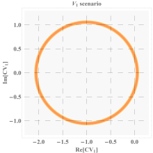
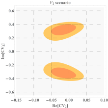
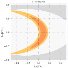
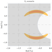
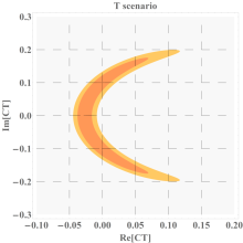
Figure 1: Constraints on the Wilson coefficients by the $b\to c\tau\nu$ data at $1\sigma$ and $2\sigma$, and the limit on $\mathcal{B}(B_{c}\to\tau\nu)$. The forbidden regions by $\mathcal{B}(B_{c}\to\tau\nu)<30\%$ are in dark grey.

5.2 Analysis of Physical Observables using Model independent Approach

In this section, we present our predictions of the observables involved in $B\to D^{(\ast)}\tau\bar{\nu}_{\tau}$, such as LFU ratio $R_{D^{(\ast)}}$, longitudinal $\tau$ polarization $P_{\tau}(D^{(\ast)})$, longitudinal polarization of final state $D^{\ast}$ meson $F_{L}^{D^{\ast}}$, and $\mathcal{A}^{\text{FB}}_{D^{(\ast)}}$, all within model independent scenario. Furthermore, we also provide the predictions using normalized angular coefficients $\langle I\rangle$’s in $B\to D^{\ast}(\to D\pi,D\gamma)\tau\bar{\nu}_{\tau}$ decays in the model-independent approach. In a model-independent approach, a global fit is performed on the Wilson coefficients of specific operators without assuming a particular type of new physics (NP) at the high-energy scale. The resulting Wilson coefficients in model-independent scenarios with and without imposing $\mathcal{B}(B_{c}\to\tau\nu)<30\%$ are presented in Table 2 and Table 3. Besides the values of Wilson coefficients obtained through global fit, we also present the plots of Wilson coefficients allowed by different measurements within $1\sigma$ and $2\sigma$ ranges in Figure 1. Furthermore, we use the best-fit values of the Wilson coefficients to give the predictions on the physical observables.

Table 2: Best-fit values of the Wilson coefficients in different NP scenarios without $\mathcal{B}(B_{c}\to\tau\nu)<0.3$.

NP scenario	value (without $\mathcal{B}(B_{c}\to\tau\nu)<0.3$)	$\chi^{2}/dof$	Correlation
$V_{1}$	$(1+\rm Re[C_{V_{1}}])^{2}+(\rm Im[C_{V_{1}}])^{2}=1.116(31)$	$23.56/17$	–
$V_{2}$	$-0.015(23)\pm 0.329(51)i$	$23.13/17$	$\pm 0.39$
$S_{1}$	$0.093(35)+0.000(433)i$	$31.24/17$	0
$S_{2}$	$-0.671(229)\pm 0.758(38)i$	$23.25/17$	$\pm 0.06$
$T$	$-0.009(52)\pm 0.086(113)i$	$25.50/17$	$\pm 0.99$

Table 3: Best-fit values of the Wilson coefficients in different NP scenarios with $\mathcal{B}(B_{c}\to\tau\nu)<0.3$.

NP scenario	value (with $\mathcal{B}(B_{c}\to\tau\nu)<0.3$)	$\chi^{2}/dof$	Correlation
$V_{1}$	$(1+\rm Re[C_{V_{1}}])^{2}+(\rm Im[C_{V_{1}}])^{2}=1.116(31)$	$23.56/17$	–
$V_{2}$	$-0.015(23)\pm 0.329(51)i$	$23.13/17$	$\pm 0.39$
$S_{1}$	$0.093(35)+0.000(433)i$	$31.24/17$	0
$S_{2}$	$-0.301(327)\pm 0.655(189)i$	$25.95/17$	$\mp 0.97$
$T$	$-0.009(52)\pm 0.086(113)i$	$25.50/17$	$\pm 0.99$

The predicted numerical values of the above mentioned physical observables are presented in Tables 4-7. The errors given in these tables arise due to hadronic uncertainties as well as from Wilson coefficients. Compared to that of SM, each of the NP scenarios except $S_{1}$ can explain the data of $R_{D^{(\ast)}}$. The polarization observables $P_{\tau}(D),P_{\tau}(D^{\ast})$, $F^{D^{\ast}}_{L}$, $\mathcal{A}^{\text{FB}}_{D^{(\ast)}}$, and the normalized angular coefficients $\langle I\rangle$’s arising from the four-fold distributions given in Eqs. (17) and (27), will be useful to discriminate different NP scenarios at the incoming and future collider experiments, such as Belle-II and LHCb. Among the above observables, $P_{\tau}(D^{\ast})$ and $F^{D^{\ast}}_{L}$ have already been measured at Belle [57, 67, 68] as listed in Table 1, while $P_{\tau}(D)$ and $\mathcal{A}^{\text{FB}}_{D^{(\ast)}}$ have not been measured yet.

Table 4: Predictions for $R_{D}$, $R_{D^{*}}$, $P_{\tau}(D)$ and $P_{\tau}(D^{*})$. The first and second uncertainties result from the form factors and the fitted Wilson coefficients.

Scenario	$R_{D}$	$R_{D^{*}}$	$P_{\tau}(D)$	$P_{\tau}(D^{*})$
SM	$0.300(3)(0)$	$0.251(1)(0)$	$0.325(3)(0)$	$-0.507(3)(0)$
$V_{1}$	$0.335(3)(10)$	$0.280(1)(8)$	$0.325(3)(0)$	$-0.507(3)(0)$
$V_{2}$	$0.324(3)(20)$	$0.285(1)(11)$	$0.325(3)(0)$	$-0.507(3)(0)$
$S_{2}$	$0.330(3)(73)$	$0.266(1)(15)$	$0.386(3)(82)$	$-0.422(5)(77)$
$T$	$0.299(3)(14)$	$0.289(1)(71)$	$0.328(3)(28)$	$-0.449(3)(92)$

Table 5: Predictions for $F_{L}^{D^{*}}$, $\mathcal{A}^{\text{FB}}_{D}$ and $\mathcal{A}^{\text{FB}}_{D^{\ast}}$. The first and second uncertainties result from the input parameters and the fitted Wilson coefficients.

Scenario	$F_{L}^{D^{*}}$	$\mathcal{A}^{\text{FB}}_{D}$	$\mathcal{A}^{\text{FB}}_{D^{\ast}}$
SM	$0.453(3)(0)$	$0.360(0)(0)$	$-0.052(4)(0)$
$V_{1}$	$0.453(3)(0)$	$0.360(0)(0)$	$-0.052(4)(0)$
$V_{2}$	$0.454(3)(2)$	$0.360(0)(0)$	$-0.013(3)(9)$
$S_{2}$	$0.484(3)(28)$	$0.205(0)(99)$	$-0.022(4)(30)$
$T$	$0.428(3)(38)$	$0.356(0)(16)$	$-0.018(3)(35)$

In most NP scenarios, the predictions for $P_{\tau}(D)$ are closer to that of SM, but in the scenario $S_{2}$, we predict the larger value of $P_{\tau}(D)$ compared to that of SM. Similarly, in most scenarios, the predictions of $P_{\tau}(D^{*})$ are also close to SM prediction, but for scenarios $S_{2}$ and $T$, the predicted value of $P_{\tau}(D^{\ast})$ is large compared to that of SM prediction, and hence the precise measurements on longitudinal $\tau$ polarizations will be useful to discriminate different NP scenarios. For the longitudinal $D^{*}$ polarization, predictions of SM and most scenarios are close to $0.46$, but in $T$ scenario the prediction is smaller than that of SM value, while in $S_{2}$ scenario the value is bigger than that of SM value. In SM and NP scenarios $V_{1}$, $V_{2}$, $\mathcal{A}^{\text{FB}}_{D}$ is predicted to be close to $0.36$, except for scenarios $S_{2}$ and $T$, where the predicted values of $\mathcal{A}^{\text{FB}}_{D}$ are smaller than the SM value. For $\mathcal{A}^{\text{FB}}_{D^{\ast}}$ only the scenario $V_{1}$ merges with SM, with the predicted value of $\mathcal{A}^{\text{FB}}_{D^{\ast}}\simeq-0.052$. However, the value of $\mathcal{A}^{\text{FB}}_{D^{\ast}}$ in other scenarios $V_{2}$, $S_{2}$, and $T$ shows departure from SM prediction. For both observables $\mathcal{A}^{\text{FB}}_{D}$ and $\mathcal{A}^{\text{FB}}_{D^{\ast}}$ the numerical values are presented in Table 5, where the predicted scenarios can be discriminated in the future and current colliders.

Table 6: Predictions of averaged values of angular observables for the $B\to D^{\ast}(\to D\pi)\tau\bar{\nu}_{\tau}$ decay, for ${V_{1}}$, ${V_{2}}$, ${P}$ and ${T}$. The first and second errors presented arise from the uncertainties of the form factors and Wilson coefficients, respectively.

	SM	${V_{1}}$	${V_{2}}$	${P}$	${T}$
$\langle I^{\pi}_{1s}\rangle$	$0.364(6)(0)$	$0.364(7)(0)$	$0.363(6)(11)$	$0.373(6)(10)$	$0.372(8)(13)$
$\langle I^{\pi}_{1c}\rangle$	$0.594(12)(0)$	$0.594(12)(0)$	$0.595(12)(1)$	$0.573(12)(20)$	$0.579(16)(27)$
$\langle I^{\pi}_{2s}\rangle$	$0.058(0)(0)$	$0.058(0)(0)$	$0.058(0)(0)$	$0.060(0)(1)$	$0.035(0)(30)$
$\langle I^{\pi}_{2c}\rangle$	$-0.151(2)(0)$	$-0.151(2)(0)$	$-0.151(2)(0)$	$-0.155(2)(4)$	$-0.10(4)(60)$
$\langle I^{\pi}_{3}\rangle$	$-0.100(2)(0)$	$-0.100(2)(0)$	$-0.101(2)(0)$	$-0.103(1)(3)$	$-0.065(1)(45)$
$\langle I^{\pi}_{4}\rangle$	$-0.127(0)(0)$	$-0.127(0)(0)$	$-0.127(0)(0)$	$-0.130(0)(3)$	$-0.082(1)(58)$
$\langle I^{\pi}_{5}\rangle$	$0.284(6)(0)$	$0.284(6)(0)$	$0.280(6)(4)$	$0.248(7)(18)$	$0.212(8)(90)$
$\langle I^{\pi}_{6s}\rangle$	$-0.217(10)(0)$	$-0.217(10)(0)$	$-0.170(10)(12)$	$-0.223(10)(6)$	$-0.134(6)(95)$
$\langle I^{\pi}_{6c}\rangle$	$0.40(11)(0)$	$0.40(9)(0)$	$0.40(9)(1)$	$0.30(8)(65)$	$0.344(9)(81)$

Table 7: Predictions of averaged values of angular observables for the $B\to D^{\ast}(\to D\gamma)\tau\bar{\nu}_{\tau}$ decay, for ${V_{1}}$, ${V_{2}}$, ${P}$ and ${T}$. The first and second errors presented arise from the uncertainties of the form factors and Wilson coefficients, respectively.

	SM	${V_{1}}$	${V_{2}}$	${P}$	${T}$
$\langle I^{\gamma}_{1s}\rangle$	$0.542(2)(0)$	$0.542(2)(0)$	$0.542(2)(5)$	$0.536(3)(8)$	$0.547(3)(8)$
$\langle I^{\gamma}_{1c}\rangle$	$0.165(5)(0)$	$0.165(5)(0)$	$0.164(5)(0)$	$0.173(5)(10)$	$0.171(5)(11)$
$\langle I^{\gamma}_{2s}\rangle$	$-0.137(1)(0)$	$-0.137(1)(0)$	$-0.137(1)(0)$	$-0.144(1)(9)$	$-0.110(3)(17)$
$\langle I^{\gamma}_{2c}\rangle$	$0.026(0)(0)$	$0.026(0)(0)$	$0.026(0)(0)$	$0.027(0)(1)$	$0.020(0)(11)$
$\langle I^{\gamma}_{3}\rangle$	$0.091(3)(0)$	$0.091(3)(0)$	$0.091(3)(0)$	$0.096(3)(5)$	$0.072(2)(38)$
$\langle I^{\gamma}_{4}\rangle$	$0.115(2)(0)$	$0.115(2)(0)$	$0.115(2)(0)$	$0.121(2)(7)$	$0.091(2)(43)$
$\langle I^{\gamma}_{5}\rangle$	$-0.257(7)(0)$	$-0.257(7)(0)$	$-0.253(7)(4)$	$-0.228(7)(17)$	$-0.221(9)(68)$
$\langle I^{\gamma}_{6s}\rangle$	$0.367(5)(0)$	$0.367(5)(0)$	$0.367(5)(0)$	$0.273(4)(62)$	$0.342(7)(50)$
$\langle I^{\gamma}_{6c}\rangle$	$-0.098(5)(0)$	$-0.098(5)(0)$	$-0.08(4)(6)$	$-0.103(5)(6)$	$-0.074(5)(44)$

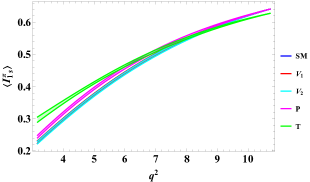
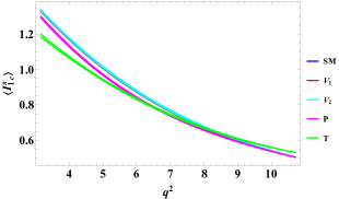
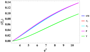
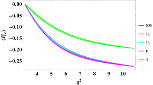
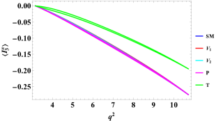
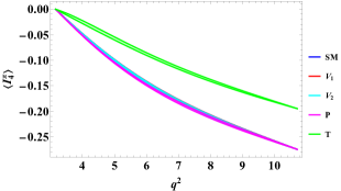
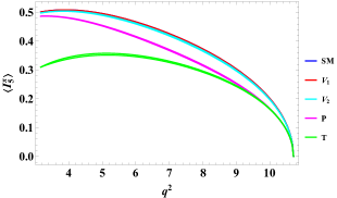
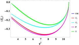
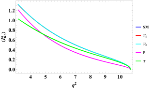
Figure 2: Angular observables $\langle I^{\pi}_{1s}\rangle$, $\langle I^{\pi}_{1c}\rangle$, $\langle I^{\pi}_{2s}\rangle$, $\langle I^{\pi}_{2c}\rangle$, $\langle I^{\pi}_{3}\rangle$, $\langle I^{\pi}_{4}\rangle$, $\langle I^{\pi}_{5}\rangle$, $\langle I^{\pi}_{6s}\rangle$, and $\langle I^{\pi}_{6c}\rangle$ for the decay $B\to D^{\ast}(\to D\pi)\tau^{-}\bar{\nu}$, in SM and in the model independent scenarios.

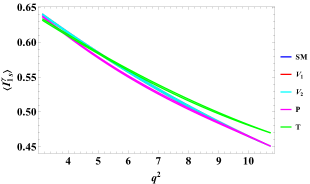
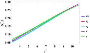
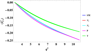
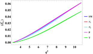
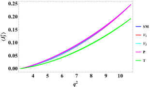
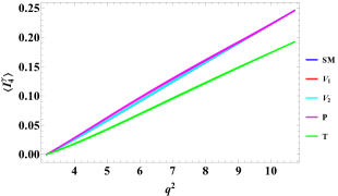
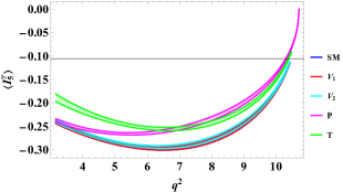
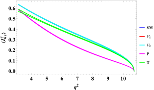
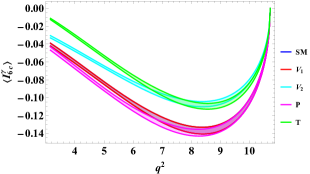
Figure 3: Angular observables $\langle I^{\gamma}_{1s}\rangle$, $\langle I^{\gamma}_{1c}\rangle$, $\langle I^{\gamma}_{2s}\rangle$, $\langle I^{\gamma}_{2c}\rangle$, $\langle I^{\gamma}_{3}\rangle$, $\langle I^{\gamma}_{4}\rangle$, $\langle I^{\gamma}_{5}\rangle$, $\langle I^{\gamma}_{6s}\rangle$, and $\langle I^{\gamma}_{6c}\rangle$ for the decay $B\to D^{\ast}(\to D\gamma)\tau^{-}\bar{\nu}$, in SM and in the model independent scenarios.

Now, we turn to discuss the phenomenological analysis of the normalized angular coefficients of $B\to D^{\ast}(\to D\pi,D\gamma)\tau\bar{\nu}_{\tau}$ decays. In Figures 2 and 3, we have plotted the normalized angular coefficients as a function of $q^{2}$ for SM and the model independent NP scenarios, whereas the averaged values of these observables are presented in Tables 6 and 7. In Figure 2, we present the angular observables $\langle I_{1s}^{\pi}\rangle$, $\langle I_{1c}^{\pi}\rangle$, $\langle I_{2s}^{\pi}\rangle$, $\langle I_{2c}^{\pi}\rangle$, $\langle I^{\pi}_{3}\rangle$, $\langle I^{\pi}_{4}\rangle$, $\langle I^{\pi}_{5}\rangle$, $\langle I_{6s}^{\pi}\rangle$ and $\langle I_{6c}^{\pi}\rangle$ for the decay $B\to D^{\ast}(\to D\pi)\tau\bar{\nu}_{\tau}$ in SM and NP model independent scenarios that exhibit vectors $V_{1}$, $V_{2}$, pseudoscalar $P$ and tensor $T$ type couplings. It is evident that the angular coefficients predictions of $\langle I_{1s}^{\pi}\rangle$, $\langle I_{1c}^{\pi}\rangle$, $\langle I_{2s}^{\pi}\rangle$, $\langle I_{2c}^{\pi}\rangle$, $\langle I^{\pi}_{3}\rangle$, $\langle I^{\pi}_{4}\rangle$, $\langle I^{\pi}_{5}\rangle$, and $\langle I_{6c}^{\pi}\rangle$ overlap with the predictions of the SM in the presence of vector-type NP couplings, $V_{1}$ and $V_{2}$. However, NP contributions from pseudoscalar ($P$) and tensor ($T$) couplings deviate significantly from the SM predictions. For the observables $\langle I_{1s}^{\pi}\rangle$ and $\langle I_{1c}^{\pi}\rangle$, the NP couplings $P$ and $T$ show significant overlap at higher $q^{2}$ values but exhibit deviations at lower $q^{2}$ values. For the angular coefficients $\langle I_{2s}^{\pi}\rangle$, $\langle I_{2c}^{\pi}\rangle$, $\langle I_{3}^{\pi}\rangle$, and $\langle I_{4}^{\pi}\rangle$, it is clear that all scenarios are closer to SM values except for the coupling $T$ which is distinguishable from SM. Furthermore, for the angular coefficients $\langle I^{\pi}_{5}\rangle$ and $\langle I^{\pi}_{6c}\rangle$, $P$ and $T$ scenarios show significant deviations from the SM predictions for almost the entire range of $q^{2}$. Lastly, for $\langle I^{\pi}_{6s}\rangle$, $V_{2}$, $P$ and $T$ scenarios predictions vary from the SM values, whereas scenario, $V_{1}$ lies very close to the SM predictions.

Figure 3, presents the angular observables $\langle I_{1s}^{\gamma}\rangle$, $\langle I_{1c}^{\gamma}\rangle$, $\langle I_{2s}^{\gamma}\rangle$, $\langle I_{2c}^{\gamma}\rangle$, $\langle I_{3}^{\gamma}\rangle$, $\langle I_{4}^{\gamma}\rangle$, $\langle I_{5}^{\gamma}\rangle$, $\langle I_{6s}^{\gamma}\rangle$ and $\langle I_{6c}^{\gamma}\rangle$ for the $B\to D^{\ast}(\to D\gamma)\tau\bar{\nu}_{\tau}$ decay in SM and model independent scenarios $V_{1}$, $V_{2}$, $P$ and $T$. For all angular observables, it is observed that the scenario $V_{1}$ and $V_{2}$ completely overlap with the SM except $\langle I_{6c}^{\gamma}\rangle$, where $V_{2}$ scenario is distinct from the SM and $V_{1}$ scenario predictions. The values within scenario $T$ are observed to be clearly distinct from SM and all other scenarios, for all angular observables, except for $\langle I^{\gamma}_{1s}\rangle$ and $\langle I^{\gamma}_{1c}\rangle$. However, for certain angular observables such as $\langle I^{\gamma}_{5}\rangle,\langle I^{\gamma}_{6s}\rangle$ and $\langle I^{\gamma}_{6c}\rangle$, scenario $T$ partially overlaps with $P$ and $V_{2}$ scenarios, respectively. Furthermore, scenario $P$ shows a clear departure from all other scenarios for the angular coefficient $\langle I^{\gamma}_{6s}\rangle$, whereas in $\langle I^{\gamma}_{6c}\rangle$ the scenarios $V_{2}$ and $T$ overlap at high $q^{2}$, while the scenarios $V_{1}$ and $P$ almost overlap for all values of $q^{2}$.

5.3 Analysis of Physical Observables Using Leptoquark Models

In this section, we analyze the physical observables for $B\to D^{\ast}(\to D\pi,D\gamma)\tau\bar{\nu}_{\tau}$ decay in SM and Leptoquark (LQ) models. There are 10 LQ models [72, 73, 74], that provide UV completion for SM fermions with left-handed neutrinos. Among them, three LQ models, namely $R_{2}$, $S_{1}$, and $U_{1}$, are presented in Table 8, along with their quantum numbers, which can possibly explain the $b\to c\tau\nu$ anomalies as discussed in Refs. [24, 75, 73, 76].

Table 8: Quantum numbers and couplings of the leptoquarks which can explain the $b\rightarrow c\tau\nu$ anomalies. Here $F\equiv 3B+L$.

	SM quantum number $[\textrm{SU}(3)\times\textrm{SU}(2)\times\textrm{U}(1)]$	$F$	Spin	Fermions coupled to
$R_{2}$	$(3,2,7/6)$	$0$	$0$	$\bar{c}_{R}\nu_{L},\bar{b}_{L}\tau_{R}$
$S_{1}$	$(\bar{3},1,1/3)$	$-2$	$0$	$\bar{b}_{L}^{c}\nu_{L},\bar{c}_{L}^{c}\tau_{L},\bar{c}_{R}^{c}\tau_{R}$
$U_{1}$	$(3,1,2/3)$	$0$	$1$	$\bar{c}_{L}\gamma_{\mu}\nu_{L},\bar{b}_{L}\gamma_{\mu}\tau_{L},\bar{b}_{R}\gamma_{\mu}\tau_{R}$

In a LQ model, the best-fit values of the NP couplings with and without imposing $\mathcal{B}(B_{c}\to\tau\nu_{\tau})$ constraint are presented in Table 9. In addition to that, we have also plotted the allowed values of Wilson coefficients, by different measurements, within $1\sigma$ and $2\sigma$ ranges, that are shown in Figure 4. The predicted values of the observables such as, $R_{D^{(\ast)}}$, $P_{\tau}(D^{(\ast)})$, $F_{L}^{D^{\ast}}$, $\mathcal{A}^{\text{FB}}_{D^{(\ast)}}$, and the normalized angular coefficients $\langle I\rangle$’s, in the three LQ models, are presented in Tables 10-13. Furthermore, the plots of the normalized angular coefficients $\langle I\rangle$’s as a function of $q^{2}$, in SM and in the LQ Models, are also presented in Figures 5-8.

Table 9: Best-fit values of the NP couplings in the leptoquark models.

LQ Type	value (with and without $\mathcal{B}(B_{c}\to\tau\nu)<0.3$)	$\chi^{2}/dof$	Correlation
$R_{2}$	$({\rm Re}[y_{L}^{c\tau}(y_{R}^{b\tau})^{*}],{\rm Im}[y_{L}^{c\tau}(y_{R}^{b\tau})^{*}])=(-0.415(166),\pm 1.271(74))$	22.45/17	$\pm 0.35$
$S_{1}$	$(y_{L}^{b\tau}(Vy_{L}^{*})^{c\tau}),y_{L}^{b\tau}(y_{R}^{c\tau})^{*})=(0.498(223),0.209(291))$	$23.01/17$	0.91
$S_{1}$	$(y_{L}^{b\tau}(Vy_{L}^{*})^{c\tau}),y_{L}^{b\tau}(y_{R}^{c\tau})^{*})=(-12.787(223),-0.209(291))$	$23.01/17$	0.91
$U_{1}$	$((Vx_{L})^{c\tau}(x_{L}^{b\tau})^{*},(Vx_{L})^{c\tau}(x_{R}^{b\tau})^{*})=(0.206(71),0.030(52))$	$23.22/17$	0.77
$U_{1}$	$((Vx_{L})^{c\tau}(x_{L}^{b\tau})^{*},(Vx_{L})^{c\tau}(x_{R}^{b\tau})^{*})=(-6.350(71),-0.030(52))$	$23.22/17$	0.77

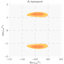
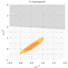
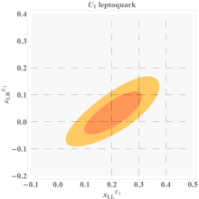
Figure 4: Constraints on the leptoquark couplings by the $b\to c\tau\nu$ data at $1\sigma$ and $2\sigma$, and the limit on $\mathcal{B}(B_{c}\to\tau\nu)$. The forbidden regions by $\mathcal{B}(B_{c}\to\tau\nu)<30\%$ are in dark grey.

Table 10: Predictions for $R_{D}$, $R_{D^{*}}$, $P_{\tau}(D)$ and $P_{\tau}(D^{*})$ in the leptoquark models. The first and second uncertainties result from the form factors and the best-fit leptoquark couplings.

LQ type	$R_{D}$	$R_{D^{*}}$	$P_{\tau}(D)$	$P_{\tau}(D^{*})$
$S_{1}$	$0.314(5)(21)$	$0.299(10)(13)$	$0.131(7)(122)$	$-0.464(7)(19)$
$R_{2}$	$0.235(4)(38)$	$0.284(11)(19)$	$0.222(3)(10)$	$-0.410(7)(21)$
$U_{1}$	$0.318(5)(20)$	$0.296(10)(13)$	$0.255(4)(73)$	$-0.509(4)(12)$

Table 11: Predictions for $F_{L}^{D^{*}}$, $\mathcal{A}^{\text{FB}}_{D}$ and $\mathcal{A}^{\text{FB}}_{D^{\ast}}$ in the leptoquark models. The first and second uncertainties result from the form factors and the best-fit leptoquark couplings.

LQ type	$F_{L}^{D^{*}}$	$\mathcal{A}^{\text{FB}}_{D}$	$\mathcal{A}^{\text{FB}}_{D^{\ast}}$
$S_{1}$	$0.485(4)(10)$	$0.377(1)(9)$	$-0.063(5)(4)$
$R_{2}$	$0.470(6)(2)$	$0.325(3)(9)$	$0.011(8)(19)$
$U_{1}$	$0.461(4)(4)$	$0.368(1)(4)$	$-0.067(6)(7)$

Table 12: Predictions of averaged values of angular observables for the $B\to D^{\ast}(\to D\pi)\tau\bar{\nu}_{\tau}$ decay in the three Leptoquark models. The first and second errors presented arise from the uncertainties of the form factors and Wilson coefficients, respectively.

	SM	${R_{2}}$ LQ model	${S_{1}}$ LQ model	${U}_{1}$ LQ model
$\langle I^{\pi}_{1s}\rangle$	$0.364(6)(0)$	$0.368(6)(4)$	$0.366(6)(3)$	$0.361(6)(3)$
$\langle I^{\pi}_{1c}\rangle$	$0.594(12)(0)$	$0.585(10)(3)$	$0.588(11)(10)$	$0.598(11)(0)$
$\langle I^{\pi}_{2s}\rangle$	$0.0583(0)(0)$	$0.0482(0)(1)$	$0.0617(0)(4)$	$0.0583(0)(0)$
$\langle I^{\pi}_{2c}\rangle$	$-0.151(2)(0)$	$-0.127(3)(4)$	$-0.159(2)(11)$	$-0.1503(2)(1)$
$\langle I^{\pi}_{3}\rangle$	$-0.099(2)(0)$	$-0.083(1)(2)$	$-0.105(2)(7)$	$-0.099(2)(0)$
$\langle I^{\pi}_{4}\rangle$	$-0.126(0)(0)$	$-0.106(1)(3)$	$-0.133(1)(9)$	$-0.126(1)(1)$
$\langle I^{\pi}_{5}\rangle$	$0.284(6)(0)$	$0.229(7)(8)$	$0.286(6)(5)$	$0.284(7)(4)$
$\langle I^{\pi}_{6s}\rangle$	$-0.217(10)(0)$	$-0.175(8)(8)$	$-0.232(11)(20)$	$-0.217(9)(2)$
$\langle I^{\pi}_{6c}\rangle$	$0.404(11)(0)$	$0.334(8)(10)$	$0.389(9)(18)$	$0.410(9)(14)$

Table 13: Predictions of averaged values of angular observables for the $B\to D^{\ast}(\to D\gamma)\tau\bar{\nu}_{\tau}$ decay, in the three LQ models. The first and second errors presented arise from the uncertainties of the form factors and Wilson coefficients, respectively.

	SM	${R_{2}}$ LQ model	${S_{1}}$ LQ model	${U}_{1}$ LQ model
$\langle I^{\gamma}_{1s}\rangle$	$0.542(2)(0)$	$0.544(2)(0)$	$0.540(3)(5)$	$0.543(3)(2)$
$\langle I^{\gamma}_{1c}\rangle$	$0.165(5)(0)$	$0.170(5)(2)$	$0.167(6)(5)$	$0.163(5)(3)$
$\langle I^{\gamma}_{2s}\rangle$	$-0.137(1)(0)$	$-0.124(1)(2)$	$-0.145(2)(10)$	$-0.136(1)(2)$
$\langle I^{\gamma}_{2c}\rangle$	$0.026(0)(0)$	$0.023(0)(0)$	$0.028(0)(0)$	$0.026(0)(0)$
$\langle I^{\gamma}_{3}\rangle$	$0.091(3)(0)$	$0.081(2)(1)$	$0.096(4)(7)$	$0.090(3)(2)$
$\langle I^{\gamma}_{4}\rangle$	$0.115(2)(0)$	$0.103(2)(2)$	$0.121(3)(8)$	$0.114(2)(2)$
$\langle I^{\gamma}_{5}\rangle$	$-0.257(7)(0)$	$-0.217(7)(7)$	$-0.260(7)(5)$	$-0.257(7)(2)$
$\langle I^{\gamma}_{6s}\rangle$	$0.367(5)(0)$	$0.311(5)(10)$	$0.00(0)(0)$	$0.373(5)(9)$
$\langle I^{\gamma}_{6c}\rangle$	$-0.098(5)(0)$	$-0.084(4)(3)$	$-0.104(5)(9)$	$-0.097(5)(2)$

From Tables 10 and 11, it is found that the most of the observables shows a departure from SM predictions. In $S_{1}$ LQ type model, the values of $R_{D}$, $R_{D^{\ast}}$, $F^{D^{\ast}}_{L}$, and $\mathcal{A}^{\text{FB}}_{D}$ indicate slight departure from SM predictions. However the values of $P_{\tau}(D),P_{\tau}(D^{\ast})$ and $\mathcal{A}^{\text{FB}}_{D^{\ast}}$ in $S_{1}$ LQ type model show a significant deviation from SM predictions. For $R_{2}$ LQ type model, the values of $R_{D}$, $P_{\tau}(D)$, $P_{\tau}(D^{\ast})$, and $\mathcal{A}^{\text{FB}}_{D^{\ast}}$ show a significant departure from SM predictions, but the values of observables such as $R_{D^{\ast}}$, $F^{D^{\ast}}_{L}$, and $\mathcal{A}^{\text{FB}}_{D^{\ast}}$ are close to SM predictions. In $U_{1}$ LQ type model, the values of observables $R_{D}$, $R_{D^{\ast}}$, $P_{\tau}(D^{\ast})$, $F^{D^{\ast}}_{L}$, and $\mathcal{A}^{\text{FB}}_{D}$ are similar to the SM values, whereas the observables $P_{\tau}(D)$ and $\mathcal{A}^{\text{FB}}_{D^{\ast}}$ deviate from SM predictions.

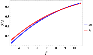
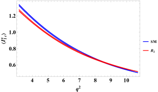
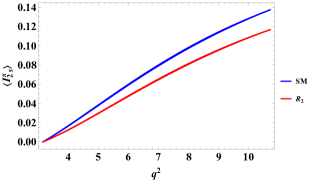
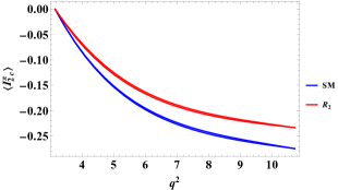
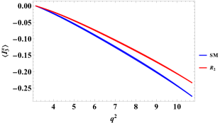
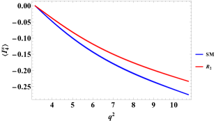
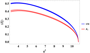
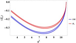
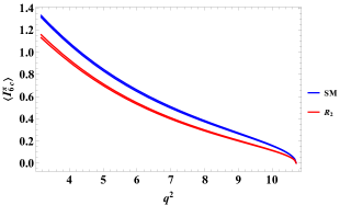
Figure 5: Angular observables $\langle I^{\pi}_{1s}\rangle$, $\langle I^{\pi}_{1c}\rangle$, $\langle I^{\pi}_{2s}\rangle$, $\langle I^{\pi}_{2c}\rangle$, $\langle I^{\pi}_{3}\rangle$, $\langle I^{\pi}_{4}\rangle$, $\langle I^{\pi}_{5}\rangle$, $\langle I^{\pi}_{6s}\rangle$, and $\langle I^{\pi}_{6c}\rangle$ for the decay $B\to D^{\ast}(\to D\pi)\tau^{-}\bar{\nu}$, in SM and in the $R_{2}$ Leptoquark model.

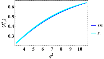
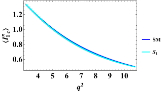
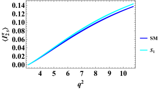
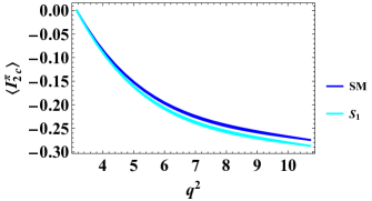
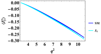
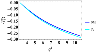
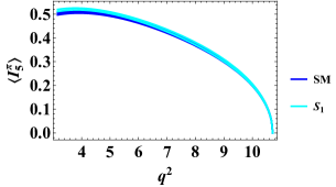
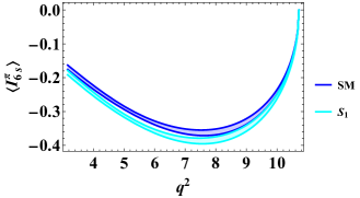
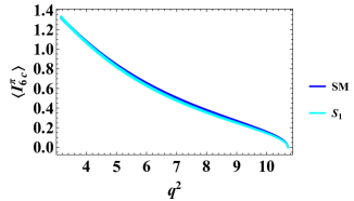
Figure 6: Angular observables $\langle I^{\pi}_{1s}\rangle$, $\langle I^{\pi}_{1c}\rangle$, $\langle I^{\pi}_{2s}\rangle$, $\langle I^{\pi}_{2c}\rangle$, $\langle I^{\pi}_{3}\rangle$, $\langle I^{\pi}_{4}\rangle$, $\langle I^{\pi}_{5}\rangle$, $\langle I^{\pi}_{6s}\rangle$, and $\langle I^{\pi}_{6c}\rangle$ for the decay $B\to D^{\ast}(\to D\pi)\tau^{-}\bar{\nu}$, in SM and in the $S_{1}$ Leptoquark model.

Now, we shall discuss the phenomenological analysis of the normalized angular coefficients $\langle I\rangle$’s for the $B\to D^{\ast}(\to D\pi)\tau\bar{\nu}_{\tau}$ decay in SM and LQ models. The angular observables $\langle I_{1s}^{\pi}\rangle$, $\langle I_{1c}^{\pi}\rangle$, $\langle I_{2s}^{\pi}\rangle$, $\langle I_{2c}^{\pi}\rangle$, $\langle I^{\pi}_{3}\rangle$, $\langle I^{\pi}_{4}\rangle$, $\langle I^{\pi}_{5}\rangle$, $\langle I_{6s}^{\pi}\rangle$ and $\langle I_{6c}^{\pi}\rangle$ in SM and in $R_{2}$ LQ model are presented in Figure 5. From the figure, it can be seen that there is a minimal discrimination between the values calculated in the SM and in $R_{2}$ LQ model for the observables $\langle I^{\pi}_{1s}\rangle$ and $\langle I^{\pi}_{1c}\rangle$ for all $q^{2}$ range. However, for the observables $\langle I^{\pi}_{2s}\rangle,\langle I^{\pi}_{2c}\rangle,\langle I^{\pi}_{3}\rangle,\langle I^{\pi}_{4}\rangle,\langle I^{\pi}_{5}\rangle,\langle I^{\pi}_{6s}\rangle$, and $\langle I^{\pi}_{6c}\rangle$, there is a significant deviation between the values calculated in the SM and the $R_{2}$ LQ model over the entire $q^{2}$ range.

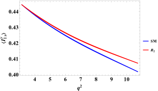
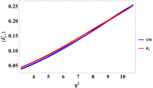
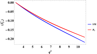
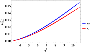
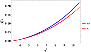
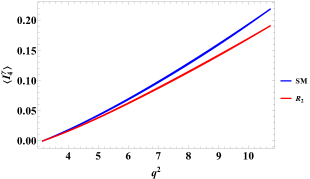
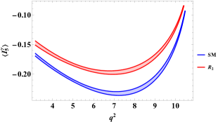
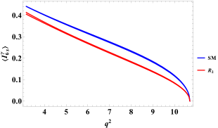
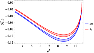
Figure 7: Angular observables $\langle I^{\gamma}_{1s}\rangle$, $\langle I^{\gamma}_{1c}\rangle$, $\langle I^{\gamma}_{2s}\rangle$, $\langle I^{\gamma}_{2c}\rangle$, $\langle I^{\gamma}_{3}\rangle$, $\langle I^{\gamma}_{4}\rangle$, $\langle I^{\gamma}_{5}\rangle$, $\langle I^{\gamma}_{6s}\rangle$, and $\langle I^{\gamma}_{6c}\rangle$ for the decay $B\to D^{\ast}(\to D\gamma)\tau^{-}\bar{\nu}$, in SM and in the $R_{2}$ Leptoquark model.

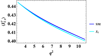
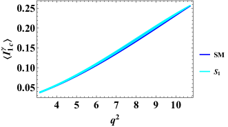
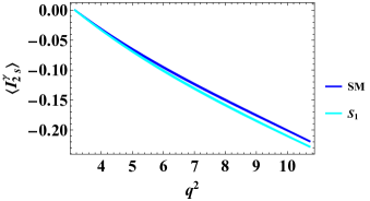
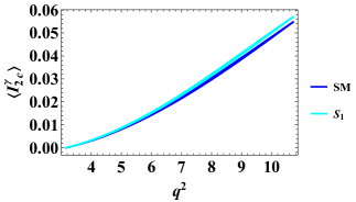
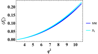
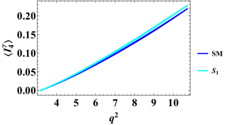
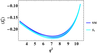
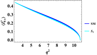
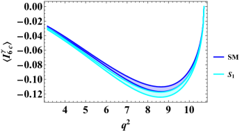
Figure 8: Angular observables $\langle I^{\gamma}_{1s}\rangle$, $\langle I^{\gamma}_{1c}\rangle$, $\langle I^{\gamma}_{2s}\rangle$, $\langle I^{\gamma}_{2c}\rangle$, $\langle I^{\gamma}_{3}\rangle$, $\langle I^{\gamma}_{4}\rangle$, $\langle I^{\gamma}_{5}\rangle$, $\langle I^{\gamma}_{6s}\rangle$, and $\langle I^{\gamma}_{6c}\rangle$ for the decay $B\to D^{\ast}(\to D\gamma)\tau^{-}\bar{\nu}$, in SM and in the $S_{1}$ Leptoquark model.

Figure 6, presents results in SM and in the $S_{1}$ LQ model. For observables $\langle I_{1s}^{\pi}\rangle$ and $\langle I_{1c}^{\pi}\rangle$, it is observed that there is a very small distinction between the values calculated within the SM and the $S_{1}$ LQ model for the whole range $q^{2}$. For observables $\langle I_{2s}^{\pi}\rangle$, $\langle I_{2c}^{\pi}\rangle$, $\langle I^{\pi}_{3}\rangle$ and $\langle I^{\pi}_{4}\rangle$, overlapping is seen between the values calculated in the SM and in the $S_{1}$ LQ model for the lower range of $q^{2}$. On the other hand, for higher $q^{2}$ values both models show small discrimination among each other. For observables $\langle I^{\pi}_{5}\rangle$ and $\langle I_{6s}^{\pi}\rangle$, the values calculated within the SM and in the $S_{1}$ LQ model overlap for the upper $q^{2}$ range, while the values are distinguishable for the lower range of $q^{2}$. The observable $\langle I_{6c}^{\pi}\rangle$ shows less or no deviation between the values calculated in the SM and $S_{1}$ LQ model. For $U_{1}$ LQ model, all the angular observables show no or small deviations from the SM predictions, therefore, we have not presented their plots, however the numerical results of the averaged angular coefficients are presented in Tables 12-13.

At last, we discuss the phenomenological analysis of the angular observables of the decay $B\to D^{\ast}(\to D\gamma)\tau\bar{\nu}$ in SM and LQ models. The results of $\langle I_{1s}^{\gamma}\rangle$, $\langle I_{1c}^{\gamma}\rangle$, $\langle I_{2s}^{\gamma}\rangle$, $\langle I_{2c}^{\gamma}\rangle$, $\langle I_{3}^{\gamma}\rangle$, $\langle I_{4}^{\gamma}\rangle$, $\langle I_{5}^{\gamma}\rangle$, $\langle I_{6s}^{\gamma}\rangle$ and $\langle I_{6c}^{\gamma}\rangle$ in SM and in $R_{2}$ LQ model, are given in Figure 7. It is found that the predictions of angular observables $\langle I_{1s}^{\gamma}\rangle$, $\langle I_{2s}^{\gamma}\rangle$, $\langle I_{2c}^{\gamma}\rangle$, $\langle I^{\gamma}_{3}\rangle$, and $\langle I^{\gamma}_{4}\rangle$, in $R_{2}$ LQ model overlap with the SM values, in the low $q^{2}$ range, however, they start deviating from the SM predictions after $q^{2}\approx 5$ $\text{GeV}^{2}$ and become more and more distinct as the $q^{2}$ range increases towards higher values. On the other hand, observable $\langle I_{1c}^{\gamma}\rangle$, in $R_{2}$ LQ model, shows no or slight deviation from the SM in the entire range of $q^{2}$. Furthermore, $R_{2}$ LQ model predictions, for the observables $\langle I^{\gamma}_{5}\rangle$, $\langle I_{6s}\rangle$, and $\langle I_{6c}^{\gamma}\rangle$, in the whole $q^{2}$ range, show identical but distinct pattern as compared to SM values, where the predictions in both models get closer to each other for the higher $q^{2}$ range and tend to merge there. Similarly, the angular observables in SM and in $S_{1}$ LQ model are presented in Figure 8. Observable $\langle I_{1s}^{\gamma}\rangle$, and $\langle I_{2s}^{\gamma}\rangle$ start to show discrimination between the values calculated within SM and $S_{1}$ LQ model from $q^{2}\sim 6$ $\text{GeV}^{2}$ and onward. For observables $\langle I_{1c}^{\gamma}\rangle$, $\langle I_{2c}^{\gamma}\rangle$, $\langle I^{\gamma}_{3}\rangle$, $\langle I^{\gamma}_{4}\rangle$, and $\langle I^{\gamma}_{6s}\rangle$, it can be seen that the values calculated within the SM and $S_{1}$ LQ model are very close to each other for the lower range of $q^{2}$. In contrast, they do indicate slight deviation from each other for the higher range of $q^{2}$. For observables $\langle I^{\gamma}_{5}\rangle$ and $\langle I_{6c}^{\gamma}\rangle$, it is observed that for lower and higher range of $q^{2}$, the values calculated within the SM and $S_{1}$ LQ model overlap but for mid range they tend to deviate from each other.

6 Conclusions

The study of $B$ meson decays provides an opportunity to probe new physics (NP) while testing the parameters of the Standard Model (SM). In particular, several semileptonic decays involving $b\to c$ transitions exhibit significant deviations from SM predictions. In this work, we analyze the $B\to D^{(*)}\tau\bar{\nu}_{\tau}$ decay within model independent framework as well as in the context of three leptoquark models. We calculate the physical observables, including the lepton flavor universality ratio $R_{D^{(*)}}$, the lepton polarization asymmetry $P_{\tau}(D^{(\ast)})$, the longitudinal helicity fraction $F^{D^{\ast}}_{L}$ of the $D^{*}$ meson, the forward-backward asymmetry $\mathcal{A}^{\text{FB}}_{D^{(*)}}$, and the normalized angular coefficients $\langle I\rangle$’s associated with the decay $B\to D^{*}(\to D\pi,D\gamma)\tau\bar{\nu}_{\tau}$. These observables are evaluated using the effective Hamiltonian formalism. We present numerical predictions for these observables within SM, model independent scenarios, and the three leptoquark models. Our findings offer valuable insights into potential new physics effects in semileptonic $b\to c$, charged current $B$-meson decays.

Based on this study, the findings reveal significant deviations in new physics scenarios from the predictions of SM for the analyzed physical observables. In model independent scenarios, it is observed that scenarios $S_{2}$ and $T$ exhibit the largest deviations from SM predictions for the observables $P_{\tau}(D)$, $P_{\tau}(D^{*})$, $F_{L}^{D^{*}}$, and $\mathcal{A}^{FB}_{D}$. For the observable $\mathcal{A}^{FB}_{D^{\ast}}$, also scenario $V_{2}$, along with $S_{2}$ and $T$, show notable deviation from SM. Regarding the normalized angular coefficients in the decay $B\to D^{\ast}(\to D\pi,D\gamma)\tau^{-}\bar{\nu}$, scenarios $P$ and $T$ show significant deviations from SM predictions. Also, Leptoquark models, $R_{2}$ and $S_{1}$, demonstrate substantial deviations from SM for various angular observables in both decay channels, $B\to D^{\ast}(\to D\pi)\tau^{-}\bar{\nu}$ and $B\to D^{\ast}(\to D\gamma)\tau^{-}\bar{\nu}$. Among these models, the $R_{2}$ leptoquark model exhibit more profound difference, whereas the $S_{1}$ model shows mild deviation from the SM prediction, in comparison. Lastly, $U_{1}$ model mostly indicates an overlap or less deviations compared to SM predictions. Future measurements of these observables at the LHC and upcoming colliders will be crucial for exploring potential new physics effects associated with these decays.

References

• [1] BaBar Collaboration, J. P. Lees et al., Evidence for an excess of $\bar{B}\to D^{(*)}\tau^{-}\bar{\nu}_{\tau}$ decays, Phys. Rev. Lett. 109 (2012) 101802, [arXiv:1205.5442].
• [2] BaBar Collaboration, J. P. Lees et al., Measurement of an Excess of $\bar{B}\to D^{(*)}\tau^{-}\bar{\nu}_{\tau}$ Decays and Implications for Charged Higgs Bosons, Phys. Rev. D 88 (2013), no. 7 072012, [arXiv:1303.0571].
• [3] Belle Collaboration, M. Huschle et al., Measurement of the branching ratio of $\bar{B}\to D^{(\ast)}\tau^{-}\bar{\nu}_{\tau}$ relative to $\bar{B}\to D^{(\ast)}\ell^{-}\bar{\nu}_{\ell}$ decays with hadronic tagging at Belle, Phys. Rev. D 92 (2015), no. 7 072014, [arXiv:1507.03233].
• [4] Belle Collaboration, S. Hirose et al., Measurement of the $\tau$ lepton polarization and $R(D^{*})$ in the decay $\bar{B}\to D^{*}\tau^{-}\bar{\nu}_{\tau}$, Phys. Rev. Lett. 118 (2017), no. 21 211801, [arXiv:1612.00529].
• [5] Belle Collaboration, S. Hirose et al., Measurement of the $\tau$ lepton polarization and $R(D^{*})$ in the decay $\bar{B}\rightarrow D^{*}\tau^{-}\bar{\nu}_{\tau}$ with one-prong hadronic $\tau$ decays at Belle, Phys. Rev. D 97 (2018), no. 1 012004, [arXiv:1709.00129].
• [6] Belle Collaboration, G. Caria et al., Measurement of $\mathcal{R}(D)$ and $\mathcal{R}(D^{*})$ with a semileptonic tagging method, Phys. Rev. Lett. 124 (2020), no. 16 161803, [arXiv:1910.05864].
• [7] LHCb Collaboration, R. Aaij et al., Measurement of the ratio of branching fractions $\mathcal{B}(\bar{B}^{0}\to D^{*+}\tau^{-}\bar{\nu}_{\tau})/\mathcal{B}(\bar{B}^{0}\to D^{*+}\mu^{-}\bar{\nu}_{\mu})$, Phys. Rev. Lett. 115 (2015), no. 11 111803, [arXiv:1506.08614]. [Erratum: Phys.Rev.Lett. 115, 159901 (2015)].
• [8] LHCb Collaboration, R. Aaij et al., Measurement of the ratio of the $B^{0}\to D^{*-}\tau^{+}\nu_{\tau}$ and $B^{0}\to D^{*-}\mu^{+}\nu_{\mu}$ branching fractions using three-prong $\tau$-lepton decays, Phys. Rev. Lett. 120 (2018), no. 17 171802, [arXiv:1708.08856].
• [9] LHCb Collaboration, R. Aaij et al., Test of Lepton Flavor Universality by the measurement of the $B^{0}\to D^{*-}\tau^{+}\nu_{\tau}$ branching fraction using three-prong $\tau$ decays, Phys. Rev. D 97 (2018), no. 7 072013, [arXiv:1711.02505].
• [10] B. Capdevila, A. Crivellin, and J. Matias, Review of semileptonic $B$ anomalies, Eur. Phys. J. ST 1 (2023) 20, [arXiv:2309.01311].
• [11] S. Bifani, S. Descotes-Genon, A. Romero Vidal, and M.-H. Schune, Review of Lepton Universality tests in $B$ decays, J. Phys. G 46 (2019), no. 2 023001, [arXiv:1809.06229].
• [12] Y. Li and C.-D. Lü, Recent Anomalies in B Physics, Sci. Bull. 63 (2018) 267–269, [arXiv:1808.02990].
• [13] Z.-R. Huang, Y. Li, C.-D. Lu, M. A. Paracha, and C. Wang, Footprints of New Physics in $b\to c\tau\nu$ Transitions, Phys. Rev. D 98 (2018), no. 9 095018, [arXiv:1808.03565].
• [14] Z.-R. Huang, E. Kou, C.-D. Lü, and R.-Y. Tang, Un-binned Angular Analysis of $B\to D^{*}\ell\nu_{\ell}$ and the Right-handed Current, Phys. Rev. D 105 (2022), no. 1 013010, [arXiv:2106.13855].
• [15] K. Cheung, Z.-R. Huang, H.-D. Li, C.-D. Lü, Y.-N. Mao, and R.-Y. Tang, Revisit to the $b\to c\tau\nu$ transition: In and beyond the SM, Nucl. Phys. B 965 (2021) 115354, [arXiv:2002.07272].
• [16] A. Crivellin, C. Greub, and A. Kokulu, Explaining $B\to D\tau\nu$, $B\to D^{*}\tau\nu$ and $B\to\tau\nu$ in a 2HDM of type III, Phys. Rev. D 86 (2012) 054014, [arXiv:1206.2634].
• [17] A. Celis, M. Jung, X.-Q. Li, and A. Pich, Sensitivity to charged scalars in ${B\to D^{(*)}\tau\nu_{\tau}}$ and ${B\to\tau\nu_{\tau}}$ decays, JHEP 01 (2013) 054, [arXiv:1210.8443].
• [18] A. Crivellin, J. Heeck, and P. Stoffer, A perturbed lepton-specific two-Higgs-doublet model facing experimental hints for physics beyond the Standard Model, Phys. Rev. Lett. 116 (2016), no. 8 081801, [arXiv:1507.07567].
• [19] M. Wei and Y. Chong-Xing, Charged Higgs bosons from the 3-3-1 models and the $\mathcal{R}(D^{(*)})$ anomalies, Phys. Rev. D 95 (2017), no. 3 035040, [arXiv:1702.01255].
• [20] C.-H. Chen and T. Nomura, Charged-Higgs on $R_{D^{(*)}}$, $\tau$ polarization, and FBA, Eur. Phys. J. C 77 (2017), no. 9 631, [arXiv:1703.03646].
• [21] P. Asadi, M. R. Buckley, and D. Shih, It’s all right(-handed neutrinos): a new $W^{\prime}$ model for the ${R}_{D^{{\left(\ast\right)}}}$ anomaly, JHEP 09 (2018) 010, [arXiv:1804.04135].
• [22] A. Greljo, D. J. Robinson, B. Shakya, and J. Zupan, $R(D^{(\ast)})$ from W${}^{\,\prime}$ and right-handed neutrinos, JHEP 09 (2018) 169, [arXiv:1804.04642].
• [23] J. D. Gómez, N. Quintero, and E. Rojas, Charged current $b\to c\tau\bar{\nu}_{\tau}$ anomalies in a general $W^{\prime}$ boson scenario, Phys. Rev. D 100 (2019), no. 9 093003, [arXiv:1907.08357].
• [24] Y. Sakaki, M. Tanaka, A. Tayduganov, and R. Watanabe, Testing leptoquark models in $\bar{B}\to D^{(*)}\tau\bar{\nu}$, Phys. Rev. D 88 (2013), no. 9 094012, [arXiv:1309.0301].
• [25] X.-Q. Li, Y.-D. Yang, and X. Zhang, Revisiting the one leptoquark solution to the R(D(∗)) anomalies and its phenomenological implications, JHEP 08 (2016) 054, [arXiv:1605.09308].
• [26] S. Bansal, R. M. Capdevilla, and C. Kolda, Constraining the minimal flavor violating leptoquark explanation of the $R_{D^{(*)}}$ anomaly, Phys. Rev. D 99 (2019), no. 3 035047, [arXiv:1810.11588].
• [27] S. Iguro, T. Kitahara, and R. Watanabe, Global fit to $b\to c\tau\nu$ anomalies as of Spring 2024, Phys. Rev. D 110 (2024), no. 7 075005, [arXiv:2405.06062].
• [28] P. Colangelo, F. De Fazio, F. Loparco, and N. Losacco, New physics couplings from angular coefficient functions of $\bar{B}\to D^{*}(D\pi)\ell^{-}\bar{\nu}_{\ell}$, Phys. Rev. D 109 (2024), no. 7 075047, [arXiv:2401.12304].
• [29] P. Colangelo, F. De Fazio, and F. Loparco, Probing New Physics with $\bar{B}\to\rho(770)\,\ell^{-}\bar{\nu}_{\ell}$ and $\bar{B}\to a_{1}(1260)\,\ell^{-}\bar{\nu}_{\ell}$, Phys. Rev. D 100 (2019), no. 7 075037, [arXiv:1906.07068].
• [30] P. Colangelo, F. De Fazio, and F. Loparco, Role of $B_{c}^{+}\to B_{s,d}^{(*)}\,\bar{\ell}\,\nu_{\ell}$ in the Standard Model and in the search for BSM signals, Phys. Rev. D 103 (2021), no. 7 075019, [arXiv:2102.05365].
• [31] T. Kapoor, Z.-R. Huang, and E. Kou, New physics search via angular distribution of $B\rightarrow D^{*}\ell{\nu}_{\ell}$ decay in the light of the new lattice data, [arXiv:2401.11636].
• [32] E. Kou, C.-D. Lü, and F.-S. Yu, Photon Polarization in the $b\to s\gamma$ processes in the Left-Right Symmetric Model, JHEP 12 (2013) 102, [arXiv:1305.3173].
• [33] J. C. Pati and A. Salam, Lepton Number as the Fourth Color, Phys. Rev. D 10 (1974) 275–289. [Erratum: Phys.Rev.D 11, 703–703 (1975)].
• [34] R. N. Mohapatra and J. C. Pati, Left-Right Gauge Symmetry and an Isoconjugate Model of CP Violation, Phys. Rev. D 11 (1975) 566–571.
• [35] R. N. Mohapatra and J. C. Pati, A Natural Left-Right Symmetry, Phys. Rev. D 11 (1975) 2558.
• [36] R. N. Mohapatra and G. Senjanovic, Neutrino Masses and Mixings in Gauge Models with Spontaneous Parity Violation, Phys. Rev. D 23 (1981) 165.
• [37] M. Blanke, A. J. Buras, K. Gemmler, and T. Heidsieck, Delta F = 2 observables and $B\to X_{q}\gamma$ decays in the Left-Right Model: Higgs particles striking back, JHEP 03 (2012) 024, [arXiv:1111.5014].
• [38] G. Barenboim, J. Bernabeu, J. Prades, and M. Raidal, Constraints on the $W_{R}$ mass and CP violation in left-right models, Phys. Rev. D 55 (1997) 4213–4221, [hep-ph/9611347].
• [39] K. Kiers, J. Kolb, J. Lee, A. Soni, and G.-H. Wu, Ubiquitous CP violation in a top inspired left-right model, Phys. Rev. D 66 (2002) 095002, [hep-ph/0205082].
• [40] J. Kalinowski, Semileptonic Decays of $B$ Mesons into $\tau\nu_{\tau}$ in a Two Higgs Doublet Model, Phys. Lett. B 245 (1990) 201–206.
• [41] W.-S. Hou, Enhanced charged Higgs boson effects in $B\to\tau\bar{\nu},\mu\bar{\nu}$ and $b\to\tau\bar{\nu}+X$, Phys. Rev. D 48 (1993) 2342–2344.
• [42] A. Crivellin, A. Kokulu, and C. Greub, Flavor-phenomenology of two-Higgs-doublet models with generic Yukawa structure, Phys. Rev. D 87 (2013), no. 9 094031, [arXiv:1303.5877].
• [43] M. Fedele, M. Blanke, A. Crivellin, S. Iguro, U. Nierste, S. Simula, and L. Vittorio, Discriminating $B\to D^{*}\ell\nu$ form factors via polarization observables and asymmetries, Phys. Rev. D 108 (2023), no. 5 055037, [arXiv:2305.15457].
• [44] Belle Collaboration, A. Abdesselam et al., Precise determination of the CKM matrix element $\left|V_{cb}\right|$ with $\bar{B}^{0}\to D^{*\,+}\,\ell^{-}\,\bar{\nu}_{\ell}$ decays with hadronic tagging at Belle, [arXiv:1702.01521].
• [45] Belle Collaboration, E. Waheed et al., Measurement of the CKM matrix element $|V_{cb}|$ from $B^{0}\to D^{*-}\ell^{+}\nu_{\ell}$ at Belle, Phys. Rev. D 100 (2019), no. 5 052007, [arXiv:1809.03290]. [Erratum: Phys.Rev.D 103, 079901 (2021)].
• [46] I. Ray and S. Nandi, Test of new physics effects in $\overline{B}\to\left({D}^{\left(\ast\right)},\pi\right){\ell}^{-}{\overline{\nu}}_{\ell}$ decays with heavy and light leptons, JHEP 01 (2024) 022, [arXiv:2305.11855].
• [47] Belle Collaboration, R. Glattauer et al., Measurement of the decay $B\to D\ell\nu_{\ell}$ in fully reconstructed events and determination of the Cabibbo-Kobayashi-Maskawa matrix element $|V_{cb}|$, Phys. Rev. D 93 (2016), no. 3 032006, [arXiv:1510.03657].
• [48] Belle Collaboration, M. T. Prim et al., Measurement of differential distributions of $B\to D^{*}\ell\bar{\nu}_{\ell}$ and implications on $|V_{cb}|$, Phys. Rev. D 108 (2023), no. 1 012002, [arXiv:2301.07529].
• [49] M. Tanaka and R. Watanabe, New physics in the weak interaction of $\bar{B}\to D^{(*)}\tau\bar{\nu}$, Phys. Rev. D 87 (2013), no. 3 034028, [arXiv:1212.1878].
• [50] Y. Sakaki, M. Tanaka, A. Tayduganov, and R. Watanabe, Probing New Physics with $q^{2}$ distributions in $\bar{B}\to D^{(*)}\tau\bar{\nu}$, Phys. Rev. D 91 (2015), no. 11 114028, [arXiv:1412.3761].
• [51] C. G. Boyd, B. Grinstein, and R. F. Lebed, Constraints on form-factors for exclusive semileptonic heavy to light meson decays, Phys. Rev. Lett. 74 (1995) 4603–4606, [hep-ph/9412324].
• [52] C. G. Boyd, B. Grinstein, and R. F. Lebed, Precision corrections to dispersive bounds on form-factors, Phys. Rev. D 56 (1997) 6895–6911, [hep-ph/9705252].
• [53] BaBar Collaboration, J. P. Lees et al., Evidence for an excess of $\bar{B}\to D^{(*)}\tau^{-}\bar{\nu}_{\tau}$ decays, Phys. Rev. Lett. 109 (2012) 101802, [arXiv:1205.5442].
• [54] BaBar Collaboration, J. P. Lees et al., Measurement of an Excess of $\bar{B}\to D^{(*)}\tau^{-}\bar{\nu}_{\tau}$ Decays and Implications for Charged Higgs Bosons, Phys. Rev. D88 (2013), no. 7 072012, [arXiv:1303.0571].
• [55] Belle Collaboration, M. Huschle et al., Measurement of the branching ratio of $\bar{B}\to D^{(\ast)}\tau^{-}\bar{\nu}_{\tau}$ relative to $\bar{B}\to D^{(\ast)}\ell^{-}\bar{\nu}_{\ell}$ decays with hadronic tagging at Belle, Phys. Rev. D92 (2015), no. 7 072014, [arXiv:1507.03233].
• [56] Belle Collaboration, Y. Sato et al., Measurement of the branching ratio of $\bar{B}^{0}\rightarrow D^{*+}\tau^{-}\bar{\nu}_{\tau}$ relative to $\bar{B}^{0}\rightarrow D^{*+}\ell^{-}\bar{\nu}_{\ell}$ decays with a semileptonic tagging method, Phys. Rev. D94 (2016), no. 7 072007, [arXiv:1607.07923].
• [57] Belle Collaboration, S. Hirose et al., Measurement of the $\tau$ lepton polarization and $R(D^{*})$ in the decay $\bar{B}\to D^{*}\tau^{-}\bar{\nu}_{\tau}$, Phys. Rev. Lett. 118 (2017), no. 21 211801, [arXiv:1612.00529].
• [58] LHCb Collaboration, R. Aaij et al., Measurement of the ratio of the $B^{0}\to D^{*-}\tau^{+}\nu_{\tau}$ and $B^{0}\to D^{*-}\mu^{+}\nu_{\mu}$ branching fractions using three-prong $\tau$-lepton decays, Phys. Rev. Lett. 120 (2018), no. 17 171802, [arXiv:1708.08856].
• [59] LHCb Collaboration, R. Aaij et al., Test of Lepton Flavor Universality by the measurement of the $B^{0}\to D^{*-}\tau^{+}\nu_{\tau}$ branching fraction using three-prong $\tau$ decays, Phys. Rev. D97 (2018), no. 7 072013, [arXiv:1711.02505].
• [60] LHCb Collaboration, R. Aaij et al., Test of lepton flavor universality using $B^{0}\to D^{*\,-}{\tau}^{+}{\nu}_{\tau}$ decays with hadronic ${\tau}$ channels, Phys. Rev. D 108 (2023), no. 1 012018, [arXiv:2305.01463]. [Erratum: Phys.Rev.D 109, 119902 (2024)].
• [61] Belle Collaboration, A. Abdesselam et al., Measurement of $\mathcal{R}(D)$ and $\mathcal{R}(D^{\ast})$ with a semileptonic tagging method, [arXiv:1904.08794].
• [62] LHCb Collaboration, R. Aaij et al., Measurement of the ratio of branching fractions $\mathcal{B}(\bar{B}^{0}\to D^{*+}\tau^{-}\bar{\nu}_{\tau})/\mathcal{B}(\bar{B}^{0}\to D^{*+}\mu^{-}\bar{\nu}_{\mu})$, Phys. Rev. Lett. 115 (2015), no. 11 111803, [arXiv:1506.08614]. [Erratum: Phys. Rev. Lett.115,no.15,159901(2015)].
• [63] LHCb Collaboration, R. Aaij et al., Measurement of the ratios of branching fractions $\mathcal{R}(D^{*})$ and $\mathcal{R}(D^{0})$, Phys. Rev. Lett. 131 (2023) 111802, [arXiv:2302.02886].
• [64] Belle-II Collaboration, I. Adachi et al., A test of lepton flavor universality with a measurement of $R(D^{*})$ using hadronic $B$ tagging at the Belle II experiment, [arXiv:2401.02840].
• [65] LHCb Collaboration, C. Chen, $b\to cl\bar{\nu}$ decays at LHCb, in 58th Rencontres de Moriond on QCD and High Energy Interactions, 5, 2024. arXiv:2405.08953.
• [66] LHCb Collaboration, R. Aaij et al., Measurement of the ratio of branching fractions $\mathcal{B}(B_{c}^{+}\,\to\,J/\psi\tau^{+}\nu_{\tau})$/$\mathcal{B}(B_{c}^{+}\,\to\,J/\psi\mu^{+}\nu_{\mu})$, Phys. Rev. Lett. 120 (2018), no. 12 121801, [arXiv:1711.05623].
• [67] Belle, Belle-II Collaboration, K. Adamczyk, Semitauonic $B$ decays at Belle/Belle II, in 10th International Workshop on the CKM Unitarity Triangle (CKM 2018) Heidelberg, Germany, September 17-21, 2018, 2019. arXiv:1901.06380.
• [68] Belle Collaboration, A. Abdesselam et al., Measurement of the $D^{\ast-}$ polarization in the decay $B^{0}\to D^{\ast-}\tau^{+}\nu_{\tau}$, in 10th International Workshop on the CKM Unitarity Triangle (CKM 2018) Heidelberg, Germany, September 17-21, 2018, 2019. arXiv:1903.03102.
• [69] LHCb Collaboration, R. Aaij et al., Observation of the decay $\Lambda_{b}^{0}\rightarrow\Lambda_{c}^{+}\tau^{-}\overline{\nu}_{\tau}$, Phys. Rev. Lett. 128 (2022), no. 19 191803, [arXiv:2201.03497].
• [70] LHCb Collaboration, R. Aaij et al., Measurement of the $D^{*}$ longitudinal polarization in $B^{0}\to D^{*-}\tau^{+}\nu_{\tau}$ decays, [arXiv:2311.05224].
• [71] CMS Collaboration, F. Riti, Recent CMS results on flavor anomalies and lepton flavor violation, PoS EPS-HEP2023 (2024) 334.
• [72] Particle Data Group Collaboration, M. Tanabashi et al., Review of Particle Physics, Phys. Rev. D98 (2018), no. 3 030001.
• [73] I. Dor$\check{\textrm{s}}$ner, S. Fajfer, A. Greljo, J. F. Kamenik, and N. Ko$\check{\textrm{s}}$nik, Physics of leptoquarks in precision experiments and at particle colliders, Phys. Rept. 641 (2016) 1–68, [arXiv:1603.04993].
• [74] W. Buchmuller, R. Ruckl, and D. Wyler, Leptoquarks in Lepton - Quark Collisions, Phys. Lett. B191 (1987) 442–448. [Erratum: Phys. Lett.B448,320(1999)].
• [75] A. Angelescu, D. Becirevic, D. A. Faroughy, and O. Sumensari, Closing the window on single leptoquark solutions to the $B$-physics anomalies, JHEP 10 (2018) 183, [arXiv:1808.08179].
• [76] S. Iguro, T. Kitahara, Y. Omura, R. Watanabe, and K. Yamamoto, D polarization vs. ${R}_{D^{\left(\ast\right)}}$ anomalies in the leptoquark models, JHEP 02 (2019) 194, [arXiv:1811.08899].