11email: jsanz@cab.inta-csic.es 22institutetext: Instituto de Astrofísica de Andalucía (IAA-CSIC), Glorieta de la Astronomía s/n, E-18008 Granada, Spain 33institutetext: Thüringer Landessternwarte Tautenburg, Sternwarte 5, D-07778 Tautenburg, Germany 44institutetext: Institut für Astrophysik und Geophysik, George-August-Universität, Friedrich-Hund-Platz 1, D-37077 Göttingen, Germany 55institutetext: Instituto de Astrofísica de Canarias (IAC), E-38205 La Laguna, Tenerife, Spain 66institutetext: Departamento de Astrofísica, Universidad de La Laguna (ULL), E-38206 La Laguna, Tenerife, Spain 77institutetext: Landessternwarte, Zentrum für Astronomie der Universität Heidelberg, Königstuhl 12, D-69117 Heidelberg, Germany 88institutetext: Institut de Ciències de l’Espai (ICE, CSIC), Campus UAB, Can Magrans s/n, E-08193 Bellaterra, Barcelona, Spain 99institutetext: Institut d’Estudis Espacials de Catalunya (IEEC), E-08860 Castelldefels, Barcelona, Spain
Connection between planetary He i 10830 Å absorption and extreme-ultraviolet emission of planet-host stars
Abstract
Context. The detection of the He i 10830 Å triplet in exoplanet atmospheres has opened a new window for probing planetary properties, including atmospheric escape. Unlike Lyman , the triplet is significantly less affected by interstellar medium (ISM) absorption. Sufficient X-ray and extreme ultraviolet (XUV) stellar irradiation may trigger the formation of the He i triplet via photoionization and posterior recombination processes in the planet atmospheres. Only a weak trend between stellar XUV emission and the planetary He i strength has been observed so far.
Aims. We aim to confirm this mechanism for producing near-infrared He i absorption in exoplanetary atmospheres by examining a substantial sample of planetary systems.
Methods. We obtained homogeneous measurements of the planetary He i line equivalent width and consistently computed the stellar XUV ionizing irradiation. Our first step was to derive new coronal models for the planet-host stars. We used updated data from the X-exoplanets database, archival X-ray spectra of M-type stars (including AU Mic and Proxima Centauri), and new XMM-Newton X-ray data recently obtained for the CARMENES project. These data were complemented at longer wavelengths with publicly available HST, FUSE, and EUVE spectra. A total of 75 stars are carefully analyzed to obtain a new calibration between X-ray and extreme ultraviolet (EUV) emission.
Results. Two distinct relationships between stellar X-ray emission (5–100 Å) and EUVH (100–920 Å) or EUVHe (100–504 Å) radiation are obtained to scale the emission from late-type (F to M) stellar coronae. A total of 48 systems with reported planetary He i 10830 Å studies, including 21 positive detections and 27 upper limits, exhibit a robust relationship between the strength of the planetary He i feature and the ionizing XUVHe received by the planet, corrected by stellar and planetary radii, as well as the planet’s gravitational potential. Some outliers could be explained by a different atmospheric composition or the lack of planetary gaseous atmospheres. This relation may serve as a guide to predict the detectability of the He i 10830 Å absorption in exoplanet atmospheres.
Key Words.:
planetary systems – stars: coronae – X-rays: stars – planets and satellites: atmospheres1 Introduction
The detection of atmospheric features in transiting exoplanets has become the best approach to understanding the composition and evolution of their atmospheres. The earliest detection reports were made for Na i (Charbonneau et al., 2002) and H i Lyman (Vidal-Madjar et al., 2003), both in HD~209458~b. A number of atomic and molecular species have been detected since then (e.g., Madhusudhan, 2019, and references therein). It is remarkable that helium, the second most abundant element in stars and in Solar System planets such as Jupiter or Saturn, was not detected until 2018. Theoretical works (Seager & Sasselov, 2000) have predicted the possibility to detect the He i infrared triplet at 10830 Å in the atmosphere of transiting exoplanets. An attempt to detect this feature was made by Sasselov & Sanz-Forcada in 2000 and 2001, using the NASA Infrared Telescope Facility (IRTF), but no feature was detected due to bad weather conditions in both campaigns combined with insufficient instrument sensitivity. Moutou et al. (2003) used VLT/ISAAC to search for the same feature, but no detection was made either. During the following years the search for atmospheric features focused on other species. The idea of observing exoplanet atmospheres using the He i 10830 line was resurrected by Oklopčić & Hirata (2018). The line was soon detected independently by three different groups (Spake et al., 2018; Nortmann et al., 2018; Allart et al., 2018), and two more detections were reported in the same year (Mansfield et al., 2018; Salz et al., 2018). Nortmann et al. (2018) also identified, as proposed by Seager & Sasselov (2000), that in exoplanet atmospheres the line formation is directly related to the incoming stellar irradiation in the XUV band at Å, with 504 Å being the wavelength corresponding to the first ionization energy of He.
The neutral helium atom possesses two types of configurations, namely, orthohelium, and parahelium, corresponding to different sets of energy levels. In orthohelium, the most conspicuous line is actually a triplet, at 10830 Å111Lines at 10829.09, 10830.25, 10830.34 Å in the air, and 10832.06, 10833.22, 10833.31 Å in vacuum.. This triplet is associated with a less intense optical triplet at 5876 Å. The formation of these triplets has long been studied in both massive or low-mass stars. Two mechanisms have been proposed to explain the formation of the triplets: (i) collisional excitation from the singlet (parahelium) levels may populate the ground level of the triplet (orthohelium), allowing for the formation of the triplet lines at 10830 and 5876 Å. A high temperature ( K) is required for this mechanism to operate. Alternatively, in a colder environment, (ii) the He i atom can be radiatively ionized with EUV photons ( Å) that would soon recombine into neutral atoms, some of them populating the triplet lower levels in a de-excitation cascade (photoionization-recombination mechanism). Examples of the first mechanism are present in stellar winds observed in the G2 I supergiant Aqr (Dupree et al., 1992). The second mechanism is thought to be responsible for the formation of the line in stellar chromospheres of late-type stars (e.g., Zarro & Zirin, 1986), which receive EUV photons from their coronae. In this case, a balance of the two mechanisms could occur in dwarfs because of the high temperatures and density reached in their chromospheres (Andretta & Giampapa, 1995; Sanz-Forcada & Dupree, 2008).
In the case of planet atmospheres, the photoionization-recombination mechanism is likely responsible for producing this line, given their cold environment. Hence, we would expect to see a relation between the ionizing XUV irradiation of the planets and the observed He i triplet in their atmospheres. A small sample of five objects reported by Nortmann et al. (2018) seems to follow this trend, but a recent compilation of all published data on He i 10830 in exoplanets (Fossati et al., 2022) could not find such relation. Fossati et al. (2022) used the (H-ionizing) radiation in the range 5–920 Å (XUVH) as a proxy of the He-ionizing radiation. Similar non-conclusive results were found by Kirk et al. (2022), Fossati et al. (2023), and Allart et al. (2023). A further study was carried out by Zhang et al. (2023a), using a relationship between planetary mass-loss rates estimated from observations and the theoretical energy-limited mass-loss rates. These authors were able to find a rather good correlation between the XUV flux in the same range and the observed He i triplet absorption.
In this paper, we attempt to probe the correlation between ionizing stellar XUVHe (in the range 5–504 Å) irradiation and the He i triplet in exoplanets. Since high-energy photons are easily absorbed by the interstellar medium (ISM), no direct observations of spectra in the range 400–504 Å are available for stars other than the Sun and most stars do not have reliable data in the 100–400 Å range either. A coronal model is needed to estimate the stellar spectral energy distribution (SED) in the range not covered by the actual data. It is thus necessary to calculate accurate coronal models of the exoplanet host stars and to calibrate a relation allowing us to easily calculate the broadband XUVHe stellar flux. Details of the X-ray and UV observations used to prepare these models, as well as on the method employed, are described in Sects. 2 and 3. The results obtained for the objects in the sample are given in Sect. 4, together with a new scaling law to easily calculate the broadband EUV emission in the H- and He-ionizing ranges, provided that the X-ray flux is available. The different parametrizations to relate the XUVHe flux and the He i line are explored, too. In Sect. 5, we discuss the results as compared with actual He i detections observed in exoplanet atmospheres, along with the implications that they have for research on the planet atmospheres. The conclusions are given in Sect. 6. We then provide appendices to further discuss the comparison with other XUV scaling laws (Appendix A) and the relation between the He i 10830 equivalent width and the XUVHe flux (Appendix B). Tables with the observing logs and main results are found in Appendix C. In Appendix D we include the tables with X-rays and UV line fluxes, along with the figures and tables providing results of the coronal models.
2 Observations
We were granted XMM-Newton Director Discretionary Time (DDT, prop. IDs #101704 and #106917, PI Sanz-Forcada), and Guest Observer time (prop. ID #092312, PI Sanz-Forcada) to observe a sample of planet-hosting stars suitable for a search of the He i 10830 triplet with the Calar Alto high-Resolution search for M dwarfs with Exoearths with Near-infrared and optical Echelle Spectrographs (CARMENES Quirrenbach et al., 2014). XMM-Newton simultaneously operates two high-spectral resolution detectors (RGS, 6–38 Å, /100–500, den Herder et al., 2001) and three European Photon Imaging Camera (EPIC-PN and EPIC-MOS) detectors (sensitivity range 0.1–15 keV and 0.2–10 keV, respectively, 20–50, Turner et al., 2001; Strüder et al., 2001). XMM-Newton also includes an optical monitor (OM). We did not use the OM data in this work because the light in its UV filters is severely contaminated with stellar photospheric emission (Orell-Miquel et al., 2023). The data were reduced using the XMM-Newton Science Analysis Software (SAS) v20.0, and analyzed following standard procedures within the Interactive Spectral Interpretation System (ISIS, Houck & Denicola, 2000) package. Most targets did not have enough statistics to use RGS, so EPIC data were used to obtain a discrete (one to three temperatures) fit to the spectra.
Some objects were also observed with the Chandra X-ray observatory (Weisskopf et al., 2002). The High Energy Transmission Grating Spectrograph (HETGS) contains two gratings, HEG (High Energy Grating, 1.5–15 Å, 120–1200), and MEG (Medium Energy Grating 3–30 Å, 60–1200), which operate simultaneously, permitting the further analysis of the data with different spectral resolutions. The Low Energy Transmission Grating Spectrograph (LETGS, 3–175 Å, 60–1000) was used in combination with the High Resolution Camera (HRC-S). The positive and negative orders were summed for the flux measurements. Lines formed in the first dispersion order, but contaminated with contribution from higher dispersion orders, were not employed in the analysis. We also used the Advanced CCD Imaging Spectrometer (ACIS, 20–50) with no grating. Standard reduction tasks present in the CIAO v4.14 package were employed in the reduction of data retrieved from the Chandra archive and the extraction of the HEG and MEG spectra. All objects observed in X-rays are listed in Table 3. We complemented our sample with the objects in the database X-exoplanets222http://sdc.cab.inta-csic.es/xexoplanets/jsp/homepage.jsp (Sanz-Forcada et al. 2011, hereafter SF11, ), which were reanalyzed for this work as explained in Sect. 3. New XMM-Newton observations were included for a few targets of the X-exoplanets original sample (Table 3): GJ~436, GJ~674, HD~27442, HD~75289, HD~108147, HD~189733, and HD~190360. In targets with more than one XMM-Newton observation, we combined all the data to improve the quality of the EPIC spectra used in the fitting. Two objects formerly detected only with ROSAT, or with lower quality Chandra spectra, have now XMM-Newton observations (GJ~832, and $υ$~And). In the case of $ι$~Hor we used the coronal model from Sanz-Forcada et al. (2019). A few more targets were added to the sample, either because they are interesting M stars hosting exoplanets (e.g., TRAPPIST-1) because they have been surveyed searching for the He i 10830 triplet or because they can be used to establish a better relation between X-rays and EUV, such as V1298 Tau (Maggio et al., 2023).
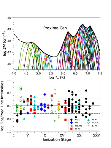
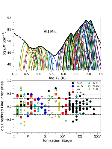
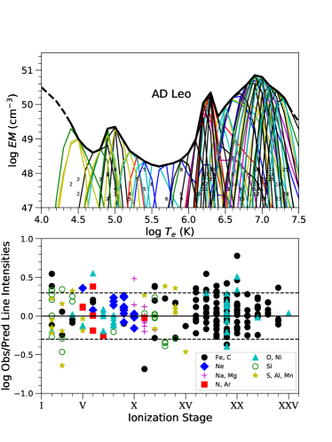
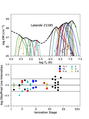
Five special cases of M dwarfs, Proxima~Cen, AU~Mic, AD Leo, Lalande 21185 (GJ~411, HD 95735), and GJ 674, were analyzed in detail using high-resolution X-ray spectra from the XMM-Newton or the Chandra archives. The use of information from individual spectral lines greatly improves the quality of the coronal models, as shown by Sanz-Forcada et al. (2003b). In these cases, we also included UV spectra (see below). Although the light curves of these targets indicate the possible presence of stellar flares, we preferred to use the combined data of quiescent and flaring states, as we understand that this reflects better the average activity of the star. In the case of Proxima Cen, it was necessary to correct for the radial velocity of the different datasets to co-add the RGS spectra333The XMM-Newton pointings were not always properly corrected for the proper motion of the star, resulting in small radial velocity shifts between different datasets.. Besides these five stars, a few targets for which we have only low-resolution XMM-Newton/EPIC or Chandra/ACIS spectra were analyzed including high-resolution UV spectra from: Hubble Space Telescope (HST) Space Telescope Imaging Spectrograph (STIS, Kimble et al., 1998)444Sensitivity ranges and resolution of the gratings: E140M 1144–1710 Å, ; G140L 1150–1730 Å, 960–1440; G140M 1140–1740 Å, 11,400–17,400 or Cosmic Origins Spectrograph (COS, Osterman et al., 2011)555Sensitivity ranges and resolution in the gratings: G130M 900–1450 Å, 12,000–17,000; G160M 1360–1775 Å, 13,000–20,000; Far Ultraviolet Spectroscopic Explorer (FUSE, 905–1187 Å, 15,000–20,000, Moos et al., 2000); and Extreme Ultraviolet Explorer (EUVE, 70–750 Å, 200–400, Haisch et al., 1993), as listed in Table 4. Extracted spectra from HST and FUSE were obtained through the Mikulski Archive for Space Telescopes (MAST), while EUVE spectra were reduced from the raw data to improve data quality, using the Image Reduction and Analysis Facility (IRAF) EUV standard tools. We also add to this list the X-ray measurements from $τ$~Boo (Maggio et al., 2011), now complemented with HST/STIS line fluxes, to extend the coronal model to transition region temperatures (down to K).
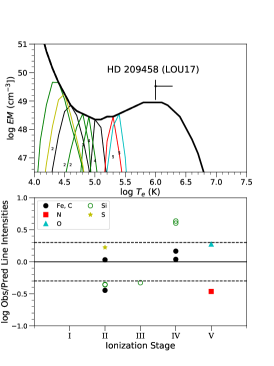
The HD 209458 and HD 189733 data were reanalyzed since Sanz-Forcada et al. (2010) to improve the results. In both cases, all the available XMM-Newton/EPIC data are combined. In the case of HD 209458 the data analysis was limited to the spectral range 0.3–8 keV to improve the statistics of the spectral fitting, which is now characterized by S/N=3.2. The data of both stars were complemented with HST/COS, as detailed by Lampón et al. (2020, 2021). In the latter case, we also fixed a software bug that led us to overestimate the flux in the EUV range and further made a more accurate analysis of the abundance pattern in the entire temperature range. New updated values of broadband EUV fluxes are made available in Table 5. All these new fluxes supersede measurements formerly reported in CARMENES papers (e.g., Nortmann et al., 2018; Lampón et al., 2021, 2023) or in Chadney et al. (2015) for the cases of AU Mic and AD Leo.
3 Methodology
We made use of coronal models to produce synthetic XUV spectra. To do so, we first calculated the volume emission measure () at different coronal temperatures using the X-ray spectra, with as defined by Brickhouse & Dupree (1998), where and are electron and hydrogen densities, respectively. The ISIS package and the Astrophysics Plasma Emission Database (APED, Smith et al., 2001) were used to fit the low resolution spectra, and to measure spectral line fluxes in high resolution spectra. We reanalyzed all the X-ray spectra included in SF11 to account for the updated stellar distances provided by Gaia DR3 (Gaia Collaboration et al., 2023) and used ATOMDB v3.0.9 in the spectral fitting and further coronal modeling. The flux of the C iii multiplet at Å is measured as one line, and its theoretical flux is evaluated using Raymond (1988) atomic data instead of ATOMDB666The fluxes of this multiplet, calculated with current version of ATOMDB, do not match those of the observed counterparts. The X-ray luminosity was calculated in the 0.12–2.48 keV band (5–100 Å), similar to the ROSAT/PSPC standard band, by global fitting of the XMM-Newton/EPIC or Chandra/ACIS low resolution spectra. The spectral fit was used to calculate a coronal model (Table ). The interstellar medium (ISM) hydrogen column density was fixed, using values from ISMTool777https://heasarc.gsfc.nasa.gov/cgi-bin/Tools/w3nh/w3nh.pl adapted to the stellar distances. The X-ray to bolometric luminosities ratio gives an indication of the activity level of the star (e.g., Pizzolato et al., 2003; Wright et al., 2011). The bolometric luminosity of the stars was calculated using the calibration by Pecaut & Mamajek (2013) based on and magnitudes888https://www.pas.rochester.edu/~emamajek/EEM_dwarf_UBVIJHK_colors_Teff.txt (accessed in March 2023), for stars with spectral types earlier than K5. The calibration from Cifuentes et al. (2020) was used for later spectral types, based on the and magnitudes.
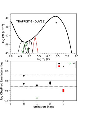
In cases with X-ray high-resolution spectra, individual line fluxes were measured considering the point spread function (PSF) of the instrument, as described by Sanz-Forcada et al. (2003b). The EUVE line fluxes were measured using standard IRAF software. The X-ray or EUV line fluxes were used to build the coronal model – namely, the emission measure distribution (EMD) – in the range of (K)5.8–7.4, while the UV line fluxes are employed for the transition region range, (K)4–5.7, including a few cases in which coronal lines were measured in the UV. The spectral line fluxes measured in the spectra and the observed-to-predicted line fluxes ratio with the resulting EMD are listed in Tables –. The EMDs are listed in Tables 12 and 13 and shown in Figs. 1–2 and 15–22. In cases where no UV spectra are available, the coronal model is extended to the transition region assuming larger error bars for this temperature range, following SF11 . The technique employed to build the EMD is described in detail by Sanz-Forcada et al. (2003b) and references therein. The basic idea is that an initial EMD is proposed, with emission measure values at each temperature in a grid of 0.1 dex in the (K) 4.0–7.5 range, and an initial set of atomic abundances; the EM is convolved with the emissivity function of each observed spectral line. The same operation is performed for any eventual blends that the observed line could have. The predicted line fluxes are then compared to the observed line fluxes and from this comparison, we changed the EMD to better match the observations in an iterative process. The abundances are calculated by doing this process for the lines of only one element (frequently, Fe) and incorporating the lines of other elements trying to partially overlap the temperature range covered by the new element and the former ones. The solution found through this process is then probed with a Monte Carlo method and modified when needed, to calculate the error bars associated with the EM at each temperature, letting the observed fluxes vary by up to in a large number of iterations.
We considered stellar abundances in the corona and transition region in the preparation of the coronal models (Tables , , ). In stars with low statistics X-ray spectra, solar photospheric abundances were used by default, except for the stellar photospheric [Fe/H] when available. In the case of abundances obtained from the global fit and the EMD, we used Fe from the global fit, and the other elements from the EMD. The level of the EMD was then based on either C or Si. In the case of HD 189733, there is a Fe iii line formed at transition region temperatures that could be used to fix the EMD level with coronal Fe abundance. As we were not confident in the quality of this line, instead we used the coronal abundances of Si, Ne, and O to fix the level of the EMD. Finally, we made use of coronal models to produce synthetic XUV SED, as detailed by SF11 , using the ISIS software. These SEDs in the 1–2800 Å range are made available in the X-exoplanets database, and in Table 1 as described in Sect. Data availability. Although some individual line fluxes may not be correct given the actual level of accuracy of ATOMDB, we are confident on the overall correctness of these SEDs in the range covered; namely, 5–920 Å. The extension to longer wavelengths should be done with care because ATOMDB has not been sufficiently tested for some of the lines at these wavelengths (e.g., the multiplet of C iii at 1176 Å). An additional difficulty may arise for stars with substantial photospheric contribution in the UV, which becomes more important for F and G stars. Emission from plasma with photospheric temperatures is not generally covered by ATOMDB.
4 Results
We calculated the broadband stellar luminosity in two different EUV bands, affecting the H ionization (EUVH, 100–920 Å) and He ionization (EUVHe, 100–504 Å), as listed in Table 5. The summed flux in the XUV bands; namely, X-rays (5–100 Å) as well as EUVH and EUVHe, were calculated at the planet orbital separation. We also calculated as a reference the mass loss rates, multiplied by the planet density (), assuming the energy-limited approach and ignoring effects related to the mass transfer through the Roche lobe:
| (1) |
where stands for the flux density in the 5–912 Å spectral range, G is the gravitational constant, and is the planet bulk density, following SF11 and references therein. Table 5 includes both the stars in the sample of Table 3 and those available in X-exoplanets as listed by SF11 . The latest were updated using new Gaia distances, as well as the new ATOMDB atomic models, as described above.
Details on some individual targets are provided, and the newly calibrated relation between X-rays and EUV flux is described next. We also explored the relation between XUVHe stellar irradiation onto the planet atmosphere and the observation of the helium infrared triplet (see Sect. 4.4).
4.1 Notes on individual targets
The sample studied in this work pays special attention to M dwarfs, the main focus of the CARMENES survey. We included some of the brightest M stars in X-rays, such as AU Mic, Proxima Cen, and AD Leo, to obtain the best possible coronal models, so that they can be widely employed in planet atmospheric modeling. The brightest objects have plenty of lines to perform an adequate coronal model and calculate the coronal abundances. Some targets are faint in X-rays and their coronal abundance analysis is more complicated, introducing some uncertainty in the balance between the EM at lower (transition region) and higher (coronal) temperatures. Some details to be considered in individual cases are discussed here. In a few stars (WASP-77, GJ~357, GJ~486, HD~149026, and TOI-836), due to the scarcity of bright spectral lines in the COS and STIS ranges, we had to include lines with S/N 3 to prepare the transition region model. We included the candidate planets AD Leo b and Barnard’s star b (Tuomi et al., 2018; Ribas et al., 2018) in the sample, although their detection has been questioned afterwards (Carleo et al., 2020; Lubin et al., 2021; Kossakowski et al., 2022).
The Barnard’s star (GJ 699) coronal model, in its high temperature component, is based on the Chandra/ACIS spectral fit, rather than on the two coronal lines measured with HST/STIS. Ne and N abundances are uncertain because we could not disentangle them from the EM values within the temperature range of line formation. Also, no relative abundances relative to Fe were calculated. Thus, the actual level of the EM in the transition region could be different. However, the observed coronal Fe lines are in agreement with the 1- fit to the Chandra value, supporting an Fe abundance that should not deviate substantially from solar photospheric values. The problem of uncertain abundances affects also GJ~1214 in N and O, in a similar temperature range.
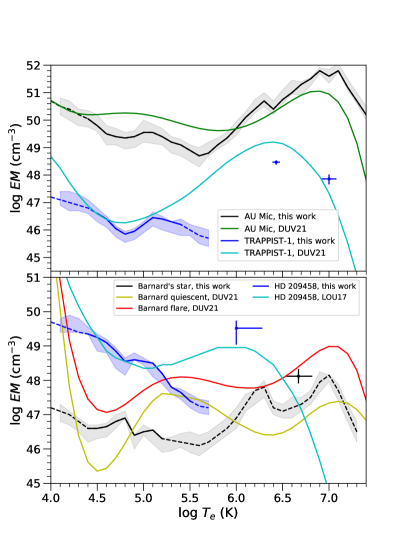
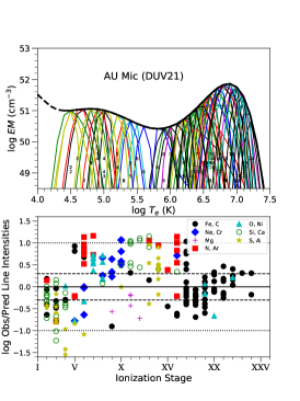
Some of the X-ray fluxes calculated in this paper differ from former publications (e.g., Louden et al., 2017; King et al., 2018). Sometimes this is due to the assumption of a different ISM absorption or coronal metallicity. We also avoid the fit of X-ray spectra below 0.3 keV, used in the mentioned work, to avoid instrumental problems such as noise in the low-energy end of EPIC spectra. Our EMD results can also be compared with those by Duvvuri et al. (2021), based on a technique that uses smooth polynomials and solar photospheric abundances to fit a differential emission measure (DEM). Their results are discrepant with ours, as discussed in Appendix A. The use of global fits to get the DEM (or EMD) from high-resolution spectra was argued against the analysis of similar data from EUVE spectra (Bowyer et al., 2000; Favata & Micela, 2003; Güdel, 2004) because it tended to produce artificial features not supported by observed line fluxes or continuum (e.g., Fig. 13 of Schrijver et al., 1995). This is a variant of the technique used by Duvvuri et al. (2021). A similar approach was adopted by Louden et al. (2017). The use of smooth polynomials imposes constrains to the DEM shape, which may not correspond to the actual DEM of the star. Another discrepancy arises when the XMM-Newton/OM UV signal is used to scale the SED modeled at UV wavelengths (Zhang et al., 2023b): the UV filters of this instrument are contaminated by stellar photospheric emission from longer wavelengths. Therefore, they cannot be used to set the UV level of emission of late-type main sequence stars (King et al., 2018; Orell-Miquel et al., 2023).
4.2 X-exoplanets 1.1: New calibration
Although it is generally advisable to calculate an individual coronal model for each stellar target, the use of scaling laws is being extensively used in the literature as a first order approach to the problem of planet photoevaporation. We thus consider it important to update the relation of X-exoplanets (SF11, ) with a better coverage of the different stellar activity regimes.
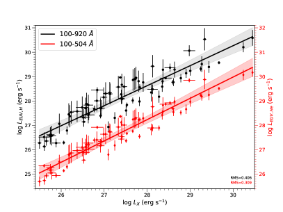
We calculated a new relation for the EUVH and EUVHe against X-ray flux. This relation allows for a fast and reliable calculation of the flux in the EUV spectral ranges, where real data are not available. The first relation of this kind was provided by SF11 , who fitted a linear relation between and , with some deviation from the linear fit at higher values. Such deviation is more evident for higher activity stars (Maggio et al., 2023). When applying a similar linear fit to out current sample, this behavior is confirmed, yielding some data dispersion. The resulting linear fits are:
| (2) |
| (3) |
where , and they are valid in the range . These fits have a Pearson’s correlation factor and 0.957, and a standard deviation of the residuals (RMS) of 0.406 and 0.309, respectively.
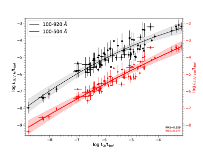
The X-ray or EUV luminosities depend on the stellar activity, as well as on the stellar size. To remove the latter dependence, we may use the stellar surface flux, with the associated uncertainties of the stellar radius (Appendix A). Instead, we fit a relation between and (Fig. 3). The use of removes the effect of the stellar size. Linear fits to these data have and 0.960, and RMS=0.380 and 0.281, respectively. A substantial bremsstrahlung continuum contribution has an increasing importance with stellar activity, and this continuum is more relevant in X-rays than at EUV wavelengths. A linear fit does not account for the dependence of broadband fluxes on this continuum. Thus a better result is found when applying a quadratic fit:
| (4) | |||||
| (5) | |||||
where . These results are valid for to , although the application of the equation for values lower than should be done with caution. Although some dispersion still exists, this approach shows a better fit (RMS=0.359 and 0.277, respectively). The remaining data dispersion might be related to deficiencies in the coronal models, such as a lack of high-resolution spectral data or problems in the calculations of stellar abundances in the corona and transition region temperature range. These problems can be mitigated by using only stars with good high-resolution spectra, both in the X-ray and UV bands. This will be subject of a future work. An intrinsic problem is also the presence of coronal activity cycles, with an X-ray amplitude that can range from a factor of to a factor of , depending on stellar activity levels. The two extreme cases observed to date are: Hor (; Sanz-Forcada et al., 2019) and the solar cycle ( to ; Orlando et al., 2001). The problem of stellar cycles can only be solved by using the average value of an already known cycle, which is the case in very few stars. The problem is also mitigated if the UV data are taken contemporaneously to the X-ray data.
4.3 Equivalent widths of the He i 10830 detections
To carry out a homogeneous analysis, we needed to revise some of the equivalent widths (s) of the previously published He detected planets with CARMENES. However, these changes were marginal. The s of planets HD 209458 b, HD 189733 b, GJ~3470~b, GJ 1214 b, WASP-69~b, and HAT-P-32~b were not changed and, thus, they were taken from Table 3 of Lampón et al. (2023). The s were integrated in the range 10831.010834.5 Å (wavelengths in vacuum). For the of WASP-76~b, the upper limit of 21.3 mÅ reported by Casasayas-Barris et al. (2021) was adopted instead of the value of 12.4 mÅ reported by Lampón et al. (2023). The latter value was obtained by integrating in a wider range, 10831.010835.5 Å, as the signal of this planet was significantly broadened and red-shifted. Except as noted, the same procedure was used for the planets with detected signal.
For WASP-52~b, the was calculated from the model fit to the data performed by Kirk et al. (2022). That fit shows an offset of 0.1%, which was subtracted. Kirk et al. (2022) also detected a small and rather noisy signal of WASP-177~b and used it to fit their model. The for the measured spectrum integrated in their spectral range is 5.8 mÅ, while that for the model is 7.5 mÅ. We took the mean value of 6.65 mÅ. For HAT-P-18~b, the was obtained from the absorption depth of 0.46% reported by Paragas et al. (2021) integrated over their bandpass of 6.35 Å. The of HD 235088 b (TOI-1430 b) was reported by Orell-Miquel et al. (2023) with a value of 9.51.1 mÅ, while our value obtained by integrating over the usual 10831.0–10834.5 Å spectral range is slightly larger, 11.1 mÅ. Zhang et al. (2023b) reported a value of 6.60.5 mÅ in a different observation.
Zhang et al. (2022a) reported a value for the of 8.60.6 mÅ in HD~73583~b (TOI 560 b). From their figures, by integrating over the spectral range described above, we obtained 7.43 mÅ. In the case of TOI-1268~b, we faced a similar problem. The by Orell-Miquel et al. (2024) is 19.1 mÅ. The value obtained with the method described above is 17.7 mÅ. We note that in this case the upper limit of the integration was slightly smaller, 10834.2 Å, due to a lack of data. The same remarks apply to TOI-2018~b, where we calculated 6.8 mÅ instead of the value of 7.8 mÅ from Orell-Miquel et al. (2024).
HAT-P-67 b seems to show a rather variable He(23S) absorption (see, e.g., Bello-Arufe et al. 2023 and Gully-Santiago et al. 2024). The CARMENES measurement, reported by Bello-Arufe et al. (2023) in their Fig. 6b, seems to have a problem as the absorption profile shows an unrealistic emission-like feature at wavelengths shorter than 10832.5 Å. That feature was likely caused by their lack of a realistic out-of-transit baseline, which prevented them from making an appropriate normalization. That is, it could be due to an increased He i absorption at bluer wavelengths towards the end of the transit. This planet was observed with a longer baseline by Gully-Santiago et al. 2024. Hence, we decided to include these measurements in our analysis. By using our method for calculating the EW, we derived from their measurements shown in Fig. 13 (the in-transit mean taken in the visit of May 2020) a value of 147 mÅ. In this case, we consider the larger value of 25 mÅ that covers the significant variability shown by the planet as “error” of the EW and not the real measured uncertainty (see the mid-transit values in Fig. 9 of the work cited above). It is worth noting that Gully-Santiago et al. 2024 measured a rather large EW of 330 mÅ at the mid transit, as well as a significant pre-transit absorption of 200 mÅ (see their Fig. 9). They stated, however, that “only a small fraction of the He i excess signal would be expected to trace the planet’s motion.” Here we focus on the absorption of the He(23S) that is being ejected from the atmosphere, not in the He(23S) that has already been ejected and forms the cloud around the planet. Then, we can estimate this absorption by taking the difference of the EW at the mid transit, from that of the material already expelled (pre-transit). This results in an absorption of 130 mÅ, which is very close to the adopted value of 147 mÅ for the mid-transit measured in May 2020.
For HAT-P-26 b, the was obtained from the absorption depth of 0.31% reported by Vissapragada et al. (2022) integrated over their full width half maximum (FWHM) bandpass of 6.35 Å. We obtained a value of 19.76.4 mÅ. The warm super-puffy TOI-1420 b planet was observed by Vissapragada et al. (2024), who obtained a high (8.5) He triplet signal, with an absorption depth of 0.671%0.079%. With those values and taking the bandwidth of their filter of 6.4 Å, we obtained an of 42.95.1 mÅ.
4.4 The relation between He i 10830 and XUV ionizing irradiation
It is expected that the formation of the He i 10830 triplet in an exoplanet atmosphere is related to the stellar irradiation on the planet by photons capable of ionizing the neutral helium atoms; namely, those with Å. The actual process of formation of these lines requires also that electrons are available in the plasma for the recombination of He atoms after the radiative ionization, and the main origin of these electrons is the radiative ionization of H atoms by photons with Å (we used 920 Å as ionization edge in our model to cover a slightly wider range). Furthermore, the stellar irradiation in this wavelength range also affects the He triplet concentration through the total density. As that radiation is responsible for the ionization of the H atmosphere, it changes the mean molecular weight and, hence, through the hydrodynamic equations, it affects the density. The stellar irradiation also affects the state of the upper atmosphere through the cooling and heating processes, which, in turn, affect the temperature and hence the hydrodynamic and the density. In addition, a third variable must be considered: the ionization of the ground level of orthohelium atoms, which takes place for Å (Kramida et al., 2023) and thus depends on the photospheric emission of the star. Although a combination of these three stellar fluxes should be considered, the right balance between the effects of the fluxes in the three bands is difficult to establish in a general way for all stars. Thus, we took the flux in the XUV range up to 504 Å (XUVHe) as a proxy of these three processes, as it is expected to be the dominant term and, in a large number of stars, this flux is well correlated with XUVH. Some attempts to derive such dependence have been undertaken999https://zenodo.org/records/13986513.
To further test this hypothesis, we collected information on the detections of the He i 10830 triplet reported to date (see below) to compare them with the XUVHe flux (Table 4). However, not all the targets in the list have a complete coronal model to calculate the XUV contribution. For those cases we calculated the flux by indirect means. The quality of the XUVHe fluxes calculated decreases in this order (as noted in Fig. 4): (1) cases with both X-ray and UV spectra, resulting in a complete coronal model; (2) targets with X-ray spectra, but no UV spectra (the coronal model with lower temperature section is extrapolated); (3) X-ray bulk flux available, such as ROSAT fluxes, and the XUVHe flux is calculated using the scaling law in Eq. 5; (4) X-ray flux determined from the rotation period and the X-ray vs. rotation relation by Wright et al. (2011), with subsequent calculation of XUVHe flux; and (5) calculation of the XUVHe flux based on blackbody emission of the stellar photosphere, for a star with unlikely or negligible coronal emission (KELT-9)101010We are more confident on our calculation assuming a blackbody emission than on the X-ray flux upper limit provided in Table 5. The XUVH flux in this star is more than four orders of magnitude higher than XUVHe flux if we assume a blackbody emission.. We also included upper limits for both the He detection and XUV flux. In case (2) the low temperature part of the coronal model is extrapolated from the high temperature section (SF11, ); upper and lower boundaries are considered during this extrapolation; thus, the XUV upper limits are based on the upper boundary coronal model, rather than on the central value used to evaluate the SED in different contexts, such as the case of WASP-12 of Czesla et al. (2024). The separate fits for the positive detections in the groups (1), (2), and (4) show consistency within the error bars with the general fit. In addition to the expected dependence of the He absorption on the stellar XUV irradiation as discussed above, we also empirically evaluated its dependence on other star-planet system parameters. The detailed discussion is found in Appendix B. Here, we include a summary of that formulation and the results.
The first point is that we choose as a proxy of the He(23S) absorption the of the absorption profile, instead of the depth (peak) of such profile, as chosen in some previous studies. The reason is that we are interested in relating the bulk He(23S) absorption by the planet atmosphere, and the is a better proxy since it is independent of the width of the absorption profile; namely, it is independent of its potential broadening by Doppler temperature and by the radial outflows of the escaping atmosphere.
The second aspect is the star’s surface. The transmission (or, equivalently, the ) is measured as a ratio of the equivalent He(23S) absorbing area of the planet atmosphere (usually expressed as the surface of a ring) and the area of the stellar disk (). If we are interested in the properties of the He(23S) absorption of a given planet atmosphere independently of the size of its host star, it seems reasonable to de-scale the measured by the stellar disk area; that is, to consider instead of just .
An additional parameter that we considered is the planet gravitational potential, , as suggested by, for instance, the theoretical model of Salz et al. (2016) and the analysis of the He(23S) absorption in diverse planets carried out by Lampón et al. (2023). According to those studies the is expected to be inversely proportional to the gravitational field because for a planet with a weaker gravitational potential, the atmosphere is escaping more easily, leading to a more extended atmosphere and, hence, a larger absorption.
A further parameter that we considered is a geometric factor related to the planet size (see Appendix B), included in a general way with , where is likely to vary between 1 and 3 depending on the star-planet system. For planets with very compressed atmospheres as, for example, the case of HD 189733 b (Salz et al., 2018; Lampón et al., 2023), the is expected to be proportional to (=1). However, for those with very extended and flat He(23S) distributions, for instance, GJ 1214 b (Lampón et al., 2023), the exponent could be larger than 2. Thus, the relationship that we considered generally takes the form (see Eq. 23):
| (6) |
We performed several tests for different relationships between and XUV fluxes, as well as for Eq. 6, using different values of the exponent of (Table ). The values collected for all planets with detected He(23S) signal and the XUVHe fluxes and other parameters listed in Table 4 were used. The stellar spectral type is also listed in the Table to alert for the possible photospheric contribution at wavelengths below 2600 Å.
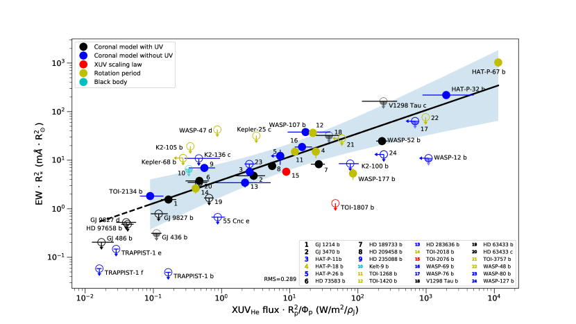
The results for the simple relationship between and (see Fig. 12) yields a decent Pearson’s correlation coefficient of , but clearly inferior to other tests described below. The correlation coefficient of the fit largely improves to a value of when scaling the by the area of the star’s disk (see Fig. 13). A further test was performed by using Eq. 6 with a value of = 1, namely, proportional to (see Fig. 13). The correlation coefficient obtained in this case is even better, reaching the value of . A subsequent test was performed by considering = 2, namely, proportional to (see Fig. 4), yielding a slightly better correlation than in the previous case, . We then proceeded to use the latter fit, which resulted in an empirical equation, excluding upper limits, of
| (7) |
where and . The is given in m, the stellar radius, , in units, in W/m2, and , which is equivalent to the inverse planet density, , in Jovian units. Error bars include the uncertainties in all of these quantities.
5 Discussion
The effects of high-energy stellar irradiation on the exoplanet atmospheres has been subject of increasing interest in recent years. The effects on the planet atmospheres are not limited to the formation of lines such as the He i 10830 triplet, but they also affect large scale phenomena such as atmospheric mass loss (atmospheric escape). The actual mass loss rate of a planet depends also on other variables different from stellar irradiation, such as atmospheric composition, stellar winds, or presence of planetary magnetic fields, and it requires an individualized approach to every case (e.g., Kubyshkina et al., 2018). However Eq. 1 is widely used to roughly compare the expected planet evolution of different cases. Since atmospheric photoevaporation should lead to atmospheric instability, a planet with a current high mass loss rate is unlikely to be habitable. The approach in Eq. 1 assumes that the atmosphere is based mainly on H, which can be appropriate for Jovian-like planets, but it may not be applicable in the case of rocky planets such as Teegarden's star b or TRAPPIST-1 b. In any case, modeling or analyzing planet atmospheres requires (as accurate as possible) knowledge of XUV stellar irradiation. With this work, we are providing new XUV synthetic SEDs for planet-hosting stars, which represents an improvement with respect to the X-exoplanets first release (SF11, ) by updating the stellar coronal models and the atomic data used to model the emission from corona and transition region. However, the number of planets hosting stars that have accurate X-ray spectra is quite limited. For those cases that do not, we include new XUV scaling laws that can be easily applied even in absence of an X-ray detection (e.g., by using the rotation period of the star, as explained in Sect. 4). For more in-depth studies, we advise users to select a star with a similar stellar spectral type and as a proxy. A more detailed work providing a grid of models of this kind will be released in the near future.
5.1 XUV scaling laws
Early works dealing with the planet photoevaporation problem assumed that the XUV emission from exoplanet host stars would be similar to the solar spectrum, scaled by the size of the star (Lecavelier Des Etangs, 2007). Alternatively, they have made use of the UV flux from the Sun and a young star for their calculations (Murray-Clay et al., 2009). A slight variation was applied by Linsky et al. (2014), France et al. (2016), and Sreejith et al. (2020), who used the solar EUV SED scaled by the overall emission in X-rays and UV of the stars. Their models were subsequently used, for instance, in Vissapragada et al. (2022), but their XUV fluxes are discrepant with ours by up to a factor of six. This approach is deficient, given that EUV spectra of active stars can be very different from those of quiet stars like the Sun (e.g., Sanz-Forcada et al., 2003a). Namekata et al. (2023) used the stellar magnetic flux and the solar spectra to extrapolate the XUV flux in active solar-like stars. The relation is calibrated mainly based on solar data, with some data coming from more active stars, along with additional uncertainties as the stellar magnetic flux is required.
A different approach was introduced by SF11 , including coronal models built with X-rays and UV data to create synthetic SEDs in the non-observed EUV spectral range. A relation between the transition region and the corona was calibrated using coronal models based on EUVE and International Ultraviolet Explorer (IUE) data, then used to complement the coronal models of stars with no UV data available. One of the results of this approach was a scaling law between X-rays and EUV luminosity that could be applied for cases where only a broadband X-ray flux is known. Chadney et al. (2015) tried to apply a more physical relation between X-rays and EUV emission by considering the activity level of the star (using the surface stellar flux, and ) in six stars, one of them based on actual solar data. King et al. (2018) followed a similar approach (without defining the used) using the same stellar data from three stars, along with solar data with some corrections applied with respect to Chadney et al. (2015). In both cases the sample was small, with most information taken from the Sun and a few very active stars. In addition, the use of stellar radius introduces further uncertainties to the problem. Johnstone et al. (2021) calibrated a relation between X-rays (5–124 Å) and the EUV surface flux in the range 100–360 Å in a sample dominated by active stars, where a new set of solar data was included. The stellar data in this case came from EUVE spectra, but with some spectra having a low quality above 180 Å (Sanz-Forcada et al., 2003a), and being usually contaminated by geocoronal emission around the He ii 304 Å line. As in the other cases, this calibration also propagates the uncertainties of the stellar radii. For the rest of the EUV range, 360–920 Å, Johnstone et al. (2021) extrapolated the ratio between these two EUV bands in the Sun to the entire range of stellar activity. While plasma in X-rays and in the EUV 100–360 Å range is mainly made of spectral lines (and continuum) formed above K, the 360–920 Å flux has a substantial contribution of lines formed at lower temperatures. Thus, it is not evident that the solar spectrum paradigm can be used for the active stars. The range of activity levels explored by Johnstone et al. (2021) included only a few low-activity stars, which are, nonetheless, still more active than some of our stars. Further comparison with these three relations is shown in Appendix A. More recently Krishnamurthy & Cowan (2024) made use of the relation between age and X-ray luminosity applied by SF11 to calculate the accumulated XUV flux over time on a planet atmosphere. While the X-ray luminosity can be used, in general terms, to estimate an approximate stellar age, the opposite is not advisable. Obtaining an accurate measurement of a stellar age is a difficult task in astrophysics; thus, using a poorly determined stellar age to calculate the X-ray and EUV fluxes may end up accumulating large uncertainties. We prefer to calculate the X-rays flux from stellar rotation if no actual measurement is available.
The new scaling law that we provide in Eq. 4 and Fig. 3 solves the limitations of past works by using coronal models for the calibration of the relation. It also uses variables that also depend on the stellar activity level to sample better the different ranges of activity. This new relation overcomes the observed problems with high activity stars (Maggio et al., 2023) and covers a wide range of activity levels. We also calculated a new relation in the range that affects the neutral helium ionization, namely, Å (Eq. 5). This allows us to better estimate the impact of the stellar high-energy irradiation on the line formation of the planetary He i 10830 triplet. Further comparisons with other recent works in the literature are provided in Appendix A.
5.2 The empirical relation between XUV and He i 10830
Earlier attempts to find an empirical relation between He i 10830 equivalent width and XUV (either at the H or the He ionization edges) have only indicated a trend, but not a clear relation (Nortmann et al., 2018; Fossati et al., 2022; Kirk et al., 2022; Allart et al., 2023). To evaluate the relation, these authors used , which is the amplitude of excess helium absorption observed, in units of the planets’ atmospheric scale heights, against the XUV stellar flux at the planet. A further study by Zhang et al. (2023a) used a different approach. They did not use the atmospheric scale height, which strictly speaking, corresponds to hydrostatic but not to hydrodynamic conditions. Instead, they plotted the mass-loss rate estimated from observations versus the theoretical energy-limited mass-loss rate (i.e., assuming a heating efficiency of 1), where the former were assumed proportional to and the latter to , where is the density of the planet calculated with the planet radius of XUV absorption (). In that way, they reached a rather good correlation.
To reduce the data dispersion in those relationships, we sought alternative parametrizations. The He i 10830 equivalent width and the XUVHe irradiation cannot directly be related with each other, as this relation neglects the impact of the stellar radius on the depth of any absorption signals measured, and the impact of the planet radius on the irradiation energy received by the planet. We therefore used the multiplied by stellar area, and the XUVHe flux multiplied by the planetary disk area and divided by the planetary gravitational potential (equivalent to a division by the planet density; see Sect. 4.4, Fig. 4, and Table 4).
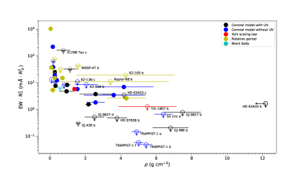
Although the observed empirical trend is clear, some dispersion is still present in the data. One reason could be the contribution of photospheric flux with Å, which ionizes the ground level of the He triplet, diminishing the expected absorption of the line. However, no deviation related to the spectral type is evident. Other relevant factors are likely related to the atmospheric composition, whether there is a primordial atmosphere, mainly composed of H and He, or the current He content is lower. Some outliers (the TRAPPIST-1 planets, 55 Cnc~e, TOI-1807~b, GJ 486 b, GJ~9827~b) lie below the He level that would be expected for their XUV irradiation: because of their Earth- and super-Earth size and high densities (Fig. 5, Table 4), they may be fully rocky without an atmosphere or they may have an atmosphere that is rather tenuous; otherwise, it may be thick, but with a high mean molecular weight. Some upper limits correspond to sub-Neptunian planets (GJ 9827 d, GJ 436 b, HD~97658~b, K2-100~b), which might have atmospheric conditions and chemical compositions that complicate the helium detection with current instrumentation. From Figs. 4 and 5, we identify that among planets with density lower than 2 g cm-3, 15 out of 28 planets were detected (%). Yet another physical reason that could explain the dispersion observed is stellar variability. The ionization levels of He i depend on the stellar XUV emission, which is highly variable, especially during flares. However, the XUV level is based on X-ray observations that are not simultaneous to the He i 10830 observations. An issue that is more related to the data acquisition and analysis is the difficulties in the measurements of exoplanets orbiting distant (i.e., faint) stars. In the particular case of WASP-177 b, Kirk et al. (2022) had some problems with systematics in the measurement of the He triplet. Another source of dispersion could be the actual dependence on the planet radius or surface, as explained in Appendix B.
6 Conclusions
Planet atmospheric photoevaporation takes place due to XUV () stellar irradiation. The He i 10830 Å triplet is used to study this phenomenon. The formation of the line in a planet atmospheric environment follows a process of ionization by photons with ¡504 Å, followed by a recombination with electrons that are mainly the result of hydrogen ionization (by photons with ¡912 Å). The main problem to evaluate the stellar flux at those wavelengths is the absorption of these photons by the ISM. To overcome this problem, we constructed coronal (and transition region) models of the star. We then calculated a synthetic SED in the whole XUV range ( Å).
We analyzed new XMM-Newton, Chandra, and EUV spectra of 50 stars, either from proprietary or archival observations. We also used high-resolution spectra to measure individual lines formed at these temperatures in 5 stars. In the case of 26 stars, we extended the analysis to the transition region temperatures by measuring UV lines in high-resolution spectra from HST and FUSE. We built detailed emission measure distributions (EMDs) for this group. We also updated the analysis of the spectra in X-exoplanets (SF11, ) using the latest Gaia distances, and the latest version of ATOMDB. The overall sample includes 100 stars hosting 163 planets, of which 75 stars have S/N, and the rest are considered upper limits. The whole sample, excluding upper limits, was then used to calculate new scaling laws for an easier calculation of the broadband fluxes that matter for the He and H ionization. A new approach to the problem was introduced by using the X-ray and EUV luminosity weighted by the bolometric luminosity. This allows us to remove effects related to stellar size, while closely considering the behavior of the scaling laws with the stellar activity. Future improvements will include more coronal high quality EMDs to reduce the dispersion observed in the data when the low-resolution X-ray spectra alone are used to model the coronae.
The newly calculated scaling laws are then used to evaluate the stellar He-ionizing irradiation in 48 exoplanets for which the He i 10830 Å triplet has been measured, including upper limits. In the cases with no X-rays measurements, we used an X-ray luminosity based on the stellar rotation period. We then checked the expected trend of the formation of this line in exoplanet atmospheres with the XUVHe stellar irradiation. A clear relation is observed, once the planet gravitational potential, along with the stellar and planetary surface are included. The remaining dispersion observed in the data can be attributed to the He content in the planet atmospheres. Some outliers, such as the TRAPPIST-1 b, e, and f planets, as well as 55 Cnc e, could be explained by the lack of planetary gaseous atmospheres. The stellar variability and the difficulties to measure the He i 10830 Å triplet in the transmission spectrum of the planet also contribute to the data dispersion. The observed relation can be used to predict the detectability of the He i 10830 Å triplet in a transiting planet.
Data availability
The SEDs modeled are listed in Table 1, only available in electronic form at the CDS via anonymous ftp to cdsarc.u-strasbg.fr (130.79.128.5) or via http://cdsweb.u-strasbg.fr/cgi-bin/qcat?J/A+A/.
Acknowledgements.
We thank the anonymous referee for the useful comments that helped improve the manuscript. We acknowledge financial support from the Agencia Estatal de Investigación (AEI/10.13039/501100011033) of the Ministerio de Ciencia e Innovación and the ERDF “A way of making Europe” through projects PID2022-137241NB-C4[1:4], PID2022-141216NB-I00, PID2021-125627OB-C31, and the Centre of Excellence “Severo Ochoa” and “María de Maeztu” awards to the Instituto de Astrofísica de Canarias (CEX2019-000920-S), Instituto de Astrofísica de Andalucía (CEX2021-001131-S) and Institut de Ciències de l’Espai (CEX2020-001058-M). We also acknowledge the support of the DFG priority program SPP 1992 “Exploring the Diversity of Extrasolar Planets” (CZ 222/5-1). We acknowledge Norbert Schartel for the observations granted as XMM-Newton Director Discretionary Time (DDT). This research has made use of the NASA’s High Energy Astrophysics Science Archive Research Center (HEASARC), and it is based on observations made with HST, FUSE, EUVE, XMM-Newton and Chandra, and obtained from the MAST data archive at the Space Telescope Science Institute, and the public archives of XMM-Newton and Chandra. CARMENES is an instrument at the Centro Astronómico Hispano en Andalucía (CAHA) at Calar Alto (Almería, Spain), operated jointly by the Junta de Andalucía and the Instituto de Astrofísica de Andalucía (CSIC). CARMENES was funded by the Max-Planck-Gesellschaft (MPG), the Consejo Superior de Investigaciones Científicas (CSIC), the Ministerio de Economía y Competitividad (MINECO) and the European Regional Development Fund (ERDF) through projects FICTS-2011-02, ICTS-2017-07-CAHA-4, and CAHA16-CE-3978, and the members of the CARMENES Consortium (Max-Planck-Institut für Astronomie, Instituto de Astrofísica de Andalucía, Landessternwarte Königstuhl, Institut de Ciències de l’Espai, Institut für Astrophysik Göttingen, Universidad Complutense de Madrid, Thüringer Landessternwarte Tautenburg, Instituto de Astrofísica de Canarias, Hamburger Sternwarte, Centro de Astrobiología and Centro Astronómico Hispano-Alemán), with additional contributions by the MINECO, the Deutsche Forschungsgemeinschaft (DFG) through the Major Research Instrumentation Programme and Research Unit FOR2544 “Blue Planets around Red Stars”, the Klaus Tschira Stiftung, the states of Baden-Württemberg and Niedersachsen, and by the Junta de Andalucía.References
- Agol et al. (2021) Agol, E., Dorn, C., Grimm, S. L., et al. 2021, PSJ, 2, 1
- Allart et al. (2019) Allart, R., Bourrier, V., Lovis, C., et al. 2019, A&A, 623, A58
- Allart et al. (2018) Allart, R., Bourrier, V., Lovis, C., et al. 2018, Science, 362, 1384
- Allart et al. (2023) Allart, R., Lemée-Joliecoeur, P. B., Jaziri, A. Y., et al. 2023, A&A, 677, A164
- Alonso-Floriano et al. (2019) Alonso-Floriano, F. J., Snellen, I. A. G., Czesla, S., et al. 2019, A&A, 629, A110
- Anders & Grevesse (1989) Anders, E. & Grevesse, N. 1989, Geochim. Cosmochim. Acta., 53, 197
- Anderson et al. (2014) Anderson, D. R., Collier Cameron, A., Delrez, L., et al. 2014, MNRAS, 445, 1114
- Anderson et al. (2017) Anderson, D. R., Collier Cameron, A., Delrez, L., et al. 2017, A&A, 604, A110
- Andretta & Giampapa (1995) Andretta, V. & Giampapa, M. S. 1995, ApJ, 439, 405
- Barragán et al. (2019) Barragán, O., Aigrain, S., Kubyshkina, D., et al. 2019, MNRAS, 490, 698
- Barragán et al. (2022) Barragán, O., Armstrong, D. J., Gandolfi, D., et al. 2022, MNRAS, 514, 1606
- Bello-Arufe et al. (2023) Bello-Arufe, A., Knutson, H. A., Mendonça, J. M., et al. 2023, AJ, 166, 69
- Bennett et al. (2023) Bennett, K. A., Redfield, S., Oklopčić, A., et al. 2023, AJ, 165, 264
- Bonomo et al. (2017) Bonomo, A. S., Desidera, S., Benatti, S., et al. 2017, A&A, 602, A107
- Borsa et al. (2019) Borsa, F., Rainer, M., Bonomo, A. S., et al. 2019, A&A, 631, A34
- Bowyer et al. (2000) Bowyer, S., Drake, J. J., & Vennes, S. 2000, ARA&A, 38, 231
- Brickhouse & Dupree (1998) Brickhouse, N. S. & Dupree, A. K. 1998, ApJ, 502, 918
- Caballero et al. (2022) Caballero, J. A., González-Álvarez, E., Brady, M., et al. 2022, A&A, 665, A120
- Carleo et al. (2020) Carleo, I., Malavolta, L., Lanza, A. F., et al. 2020, A&A, 638, A5
- Carleo et al. (2021) Carleo, I., Youngblood, A., Redfield, S., et al. 2021, AJ, 161, 136
- Casasayas-Barris et al. (2021) Casasayas-Barris, N., Orell-Miquel, J., Stangret, M., et al. 2021, A&A, 654, A163
- Chadney et al. (2015) Chadney, J. M., Galand, M., Unruh, Y. C., Koskinen, T. T., & Sanz-Forcada, J. 2015, Icarus, 250, 357
- Charbonneau et al. (2002) Charbonneau, D., Brown, T. M., Noyes, R. W., & Gilliland, R. L. 2002, ApJ, 568, 377
- Cifuentes et al. (2020) Cifuentes, C., Caballero, J. A., Cortés-Contreras, M., et al. 2020, A&A, 642, A115
- Cloutier et al. (2021) Cloutier, R., Charbonneau, D., Deming, D., Bonfils, X., & Astudillo-Defru, N. 2021, AJ, 162, 174
- Crida et al. (2018) Crida, A., Ligi, R., Dorn, C., & Lebreton, Y. 2018, ApJ, 860, 122
- Czesla et al. (2024) Czesla, S., Lampón, M., Cont, D., et al. 2024, A&A, 683, A67
- Czesla et al. (2022) Czesla, S., Lampón, M., Sanz-Forcada, J., et al. 2022, A&A, 657, A6
- Dai et al. (2023) Dai, F., Schlaufman, K. C., Reggiani, H., et al. 2023, AJ, 166, 49
- Del Zanna et al. (2002) Del Zanna, G., Landini, M., & Mason, H. E. 2002, A&A, 385, 968
- den Herder et al. (2001) den Herder, J. W., Brinkman, A. C., Kahn, S. M., et al. 2001, A&A, 365, L7
- dos Santos et al. (2020) dos Santos, L. A., Ehrenreich, D., Bourrier, V., et al. 2020, A&A, 640, A29
- Dupree et al. (1992) Dupree, A. K., Sasselov, D. D., & Lester, J. B. 1992, ApJ, 387, L85
- Duvvuri et al. (2021) Duvvuri, G. M., Sebastian Pineda, J., Berta-Thompson, Z. K., et al. 2021, ApJ, 913, 40
- Enoch et al. (2011) Enoch, B., Anderson, D. R., Barros, S. C. C., et al. 2011, AJ, 142, 86
- Favata & Micela (2003) Favata, F. & Micela, G. 2003, Space Sci. Rev., 108, 577
- Fossati et al. (2022) Fossati, L., Guilluy, G., Shaikhislamov, I. F., et al. 2022, A&A, 658, A136
- Fossati et al. (2023) Fossati, L., Pillitteri, I., Shaikhislamov, I. F., et al. 2023, A&A, 673, A37
- France et al. (2016) France, K., Loyd, R. O. P., Youngblood, A., et al. 2016, ApJ, 820, 89
- France et al. (2010) France, K., Stocke, J. T., Yang, H., et al. 2010, ApJ, 712, 1277
- Gaia Collaboration et al. (2023) Gaia Collaboration, Vallenari, A., Brown, A. G. A., et al. 2023, A&A, 674, A1
- Gaidos et al. (2020) Gaidos, E., Hirano, T., Mann, A. W., et al. 2020, MNRAS, 495, 650
- Gaidos et al. (2021) Gaidos, E., Hirano, T., Omiya, M., et al. 2021, Research Notes of the AAS, 5, 238
- Güdel (2004) Güdel, M. 2004, A&A Rev., 12, 71
- Gully-Santiago et al. (2024) Gully-Santiago, M., Morley, C. V., Luna, J., et al. 2024, AJ, 167, 142
- Haisch et al. (1993) Haisch, B., Bowyer, S., & Malina, R. F. 1993, Journal of the British Interplanetary Society, 46, 331
- Hartman et al. (2011) Hartman, J. D., Bakos, G. Á., Kipping, D. M., et al. 2011, ApJ, 728, 138
- Hébrard et al. (2013) Hébrard, G., Collier Cameron, A., Brown, D. J. A., et al. 2013, A&A, 549, A134
- Hedges et al. (2021) Hedges, C., Hughes, A., Zhou, G., et al. 2021, AJ, 162, 54
- Houck & Denicola (2000) Houck, J. C. & Denicola, L. A. 2000, in ASP Conf. Series, Vol. 216, Astronomical Data Analysis Software and Systems IX, ed. N. Manset, C. Veillet, & D. Crabtree, 591
- Johnstone et al. (2021) Johnstone, C. P., Bartel, M., & Güdel, M. 2021, A&A, 649, A96
- Kanodia et al. (2022) Kanodia, S., Libby-Roberts, J., Cañas, C. I., et al. 2022, AJ, 164, 81
- Kasper et al. (2020) Kasper, D., Bean, J. L., Oklopčić, A., et al. 2020, AJ, 160, 258
- Kimble et al. (1998) Kimble, R. A., Woodgate, B. E., Bowers, C. W., et al. 1998, ApJ, 492, L83
- King et al. (2018) King, G. W., Wheatley, P. J., Salz, M., et al. 2018, MNRAS, 478, 1193
- Kirk et al. (2022) Kirk, J., Dos Santos, L. A., López-Morales, M., et al. 2022, AJ, 164, 24
- Knutson et al. (2014) Knutson, H. A., Fulton, B. J., Montet, B. T., et al. 2014, ApJ, 785, 126
- Kosiarek et al. (2021) Kosiarek, M. R., Berardo, D. A., Crossfield, I. J. M., et al. 2021, AJ, 161, 47
- Kosiarek et al. (2019) Kosiarek, M. R., Crossfield, I. J. M., Hardegree-Ullman, K. K., et al. 2019, AJ, 157, 97
- Kossakowski et al. (2022) Kossakowski, D., Kürster, M., Henning, T., et al. 2022, A&A, 666, A143
- Kramida et al. (2023) Kramida, A., Yu. Ralchenko, Reader, J., & and NIST ASD Team. 2023, NIST Atomic Spectra Database (ver. 5.11), [Online]. Available: https://physics.nist.gov/asd [2023, December 21]. National Institute of Standards and Technology, Gaithersburg, MD.
- Krishnamurthy & Cowan (2024) Krishnamurthy, V. & Cowan, N. B. 2024, AJ, 168, 30
- Krishnamurthy et al. (2021) Krishnamurthy, V., Hirano, T., Stefánsson, G., et al. 2021, AJ, 162, 82
- Kubyshkina et al. (2018) Kubyshkina, D., Fossati, L., Erkaev, N. V., et al. 2018, ApJ, 866, L18
- Lam et al. (2017) Lam, K. W. F., Faedi, F., Brown, D. J. A., et al. 2017, A&A, 599, A3
- Lampón et al. (2020) Lampón, M., López-Puertas, M., Lara, L. M., et al. 2020, A&A, 636, A13
- Lampón et al. (2023) Lampón, M., López-Puertas, M., Sanz-Forcada, J., et al. 2023, A&A, 673, A140
- Lampón et al. (2021) Lampón, M., López-Puertas, M., Sanz-Forcada, J., et al. 2021, A&A, 647, A129
- Lecavelier Des Etangs (2007) Lecavelier Des Etangs, A. 2007, A&A, 461, 1185
- Linsky et al. (2014) Linsky, J. L., Fontenla, J., & France, K. 2014, ApJ, 780, 61
- Louden et al. (2017) Louden, T., Wheatley, P. J., & Briggs, K. 2017, MNRAS, 464, 2396
- Lubin et al. (2021) Lubin, J., Robertson, P., Stefansson, G., et al. 2021, AJ, 162, 61
- Madhusudhan (2019) Madhusudhan, N. 2019, ARA&A, 57, 617
- Maggio et al. (2023) Maggio, A., Pillitteri, I., Argiroffi, C., et al. 2023, ApJ, 951, 18
- Maggio et al. (2011) Maggio, A., Sanz-Forcada, J., & Scelsi, L. 2011, A&A, 527, A144
- Mallorquín et al. (2023) Mallorquín, M., Béjar, V. J. S., Lodieu, N., et al. 2023, A&A, 671, A163
- Mann et al. (2018) Mann, A. W., Vanderburg, A., Rizzuto, A. C., et al. 2018, AJ, 155, 4
- Mansfield et al. (2018) Mansfield, M., Bean, J. L., Oklopčić, A., et al. 2018, ApJ, 868, L34
- Masson et al. (2024) Masson, A., Vinatier, S., Bézard, B., et al. 2024, A&A, 688, A179
- Mills et al. (2019) Mills, S. M., Howard, A. W., Weiss, L. M., et al. 2019, AJ, 157, 145
- Moos et al. (2000) Moos, H. W., Cash, W. C., Cowie, L. L., et al. 2000, ApJ, 538, L1
- Moutou et al. (2003) Moutou, C., Coustenis, A., Schneider, J., Queloz, D., & Mayor, M. 2003, A&A, 405, 341
- Murray-Clay et al. (2009) Murray-Clay, R. A., Chiang, E. I., & Murray, N. 2009, ApJ, 693, 23
- Namekata et al. (2023) Namekata, K., Toriumi, S., Airapetian, V. S., et al. 2023, ApJ, 945, 147
- Nardiello et al. (2022) Nardiello, D., Malavolta, L., Desidera, S., et al. 2022, A&A, 664, A163
- Narita et al. (2017) Narita, N., Hirano, T., Fukui, A., et al. 2017, PASJ, 69, 29
- Nortmann et al. (2018) Nortmann, L., Pallé, E., Salz, M., et al. 2018, Science, 362, 1388
- Oklopčić & Hirata (2018) Oklopčić, A. & Hirata, C. M. 2018, ApJ, 855, L11
- Orell-Miquel et al. (2023) Orell-Miquel, J., Lampón, M., López-Puertas, M., et al. 2023, A&A, 677, A56
- Orell-Miquel et al. (2022) Orell-Miquel, J., Murgas, F., Pallé, E., et al. 2022, A&A, 659, A55
- Orell-Miquel et al. (2024) Orell-Miquel, J., Murgas, F., Pallé, E., et al. 2024, A&A, 689, A179
- Orlando et al. (2001) Orlando, S., Peres, G., & Reale, F. 2001, ApJ, 560, 499
- Osterman et al. (2011) Osterman, S., Green, J., Froning, C., et al. 2011, Ap&SS, 335, 257
- Palle et al. (2020) Palle, E., Nortmann, L., Casasayas-Barris, N., et al. 2020, A&A, 638, A61
- Paragas et al. (2021) Paragas, K., Vissapragada, S., Knutson, H. A., et al. 2021, ApJ, 909, L10
- Paredes et al. (2021) Paredes, L. A., Henry, T. J., Quinn, S. N., et al. 2021, AJ, 162, 176
- Pecaut & Mamajek (2013) Pecaut, M. J. & Mamajek, E. E. 2013, ApJS, 208, 9
- Pizzolato et al. (2003) Pizzolato, N., Maggio, A., Micela, G., Sciortino, S., & Ventura, P. 2003, A&A, 397, 147
- Poppenhaeger (2022) Poppenhaeger, K. 2022, MNRAS, 512, 1751
- Quirrenbach et al. (2014) Quirrenbach, A., Amado, P. J., Caballero, J. A., et al. 2014, in Society of Photo-Optical Instrumentation Engineers (SPIE) Conference Series, Vol. 9147, Society of Photo-Optical Instrumentation Engineers (SPIE) Conference Series
- Raymond (1988) Raymond, J. C. 1988, in NATO ASIC Proc. 249: Hot Thin Plasmas in Astrophysics, ed. R. Pallavicini, 3
- Rescigno et al. (2024) Rescigno, F., Hébrard, G., Vanderburg, A., et al. 2024, MNRAS, 527, 5385
- Ribas et al. (2018) Ribas, I., Tuomi, M., Reiners, A., et al. 2018, Nature, 563, 365
- Salz et al. (2018) Salz, M., Czesla, S., Schneider, P. C., et al. 2018, A&A, 620, A97
- Salz et al. (2016) Salz, M., Czesla, S., Schneider, P. C., & Schmitt, J. H. M. M. 2016, A&A, 586, A75
- Sanz-Forcada et al. (2003a) Sanz-Forcada, J., Brickhouse, N. S., & Dupree, A. K. 2003a, ApJS, 145, 147
- Sanz-Forcada & Dupree (2008) Sanz-Forcada, J. & Dupree, A. K. 2008, A&A, 488, 715
- Sanz-Forcada et al. (2003b) Sanz-Forcada, J., Maggio, A., & Micela, G. 2003b, A&A, 408, 1087
- Sanz-Forcada & Micela (2002) Sanz-Forcada, J. & Micela, G. 2002, A&A, 394, 653
- (110) Sanz-Forcada, J., Micela, G., Ribas, I., et al. 2011, A&A, 532, A6
- Sanz-Forcada et al. (2010) Sanz-Forcada, J., Ribas, I., Micela, G., et al. 2010, A&A, 511, L8
- Sanz-Forcada et al. (2019) Sanz-Forcada, J., Stelzer, B., Coffaro, M., Raetz, S., & Alvarado-Gómez, J. D. 2019, A&A, 631, A45
- Schrijver et al. (1995) Schrijver, C. J., Mewe, R., van den Oord, G. H. J., & Kaastra, J. S. 1995, A&A, 302, 438
- Seager & Sasselov (2000) Seager, S. & Sasselov, D. D. 2000, ApJ, 537, 916
- Sikora et al. (2023) Sikora, J., Rowe, J., Barat, S., et al. 2023, AJ, 165, 250
- Smith et al. (2001) Smith, R. K., Brickhouse, N. S., Liedahl, D. A., & Raymond, J. C. 2001, ApJ, 556, L91
- Spake et al. (2018) Spake, J. J., Sing, D. K., Evans, T. M., et al. 2018, Nature, 557, 68
- Sreejith et al. (2020) Sreejith, A. G., Fossati, L., Youngblood, A., France, K., & Ambily, S. 2020, A&A, 644, A67
- Strüder et al. (2001) Strüder, L., Briel, U., Dennerl, K., et al. 2001, A&A, 365, L18
- Suárez Mascareño et al. (2021) Suárez Mascareño, A., Damasso, M., Lodieu, N., et al. 2021, Nature Astronomy, 6, 232
- Triaud et al. (2013) Triaud, A. H. M. J., Anderson, D. R., Collier Cameron, A., et al. 2013, A&A, 551, A80
- Trifonov et al. (2018) Trifonov, T., Kürster, M., Zechmeister, M., et al. 2018, A&A, 609, A117
- Tuomi et al. (2018) Tuomi, M., Jones, H. R. A., Barnes, J. R., et al. 2018, AJ, 155, 192
- Turner et al. (2021) Turner, J. D., Ridden-Harper, A., & Jayawardhana, R. 2021, AJ, 161, 72
- Turner et al. (2001) Turner, M. J. L., Abbey, A., Arnaud, M., et al. 2001, A&A, 365, L27
- Turner et al. (2019) Turner, O. D., Anderson, D. R., Barkaoui, K., et al. 2019, MNRAS, 485, 5790
- Van Grootel et al. (2014) Van Grootel, V., Gillon, M., Valencia, D., et al. 2014, ApJ, 786, 2
- Vanderburg et al. (2017) Vanderburg, A., Becker, J. C., Buchhave, L. A., et al. 2017, AJ, 154, 237
- Vidal-Madjar et al. (2003) Vidal-Madjar, A., Lecavelier des Etangs, A., Désert, J.-M., et al. 2003, Nature, 422, 143
- Vissapragada et al. (2024) Vissapragada, S., Greklek-McKeon, M., Linssen, D., et al. 2024, AJ, 167, 199
- Vissapragada et al. (2022) Vissapragada, S., Knutson, H. A., Greklek-McKeon, M., et al. 2022, AJ, 164, 234
- Šubjak et al. (2022) Šubjak, J., Endl, M., Chaturvedi, P., et al. 2022, A&A, 662, A107
- Wang & Ford (2011) Wang, J. & Ford, E. B. 2011, MNRAS, 418, 1822
- Weisskopf et al. (2002) Weisskopf, M. C., Brinkman, B., Canizares, C., et al. 2002, PASP, 114, 1
- West et al. (2016) West, R. G., Hellier, C., Almenara, J. M., et al. 2016, A&A, 585, A126
- Wright et al. (2011) Wright, N. J., Drake, J. J., Mamajek, E. E., & Henry, G. W. 2011, ApJ, 743, 48
- Yee et al. (2018) Yee, S. W., Petigura, E. A., Fulton, B. J., et al. 2018, AJ, 155, 255
- Yoshida et al. (2023) Yoshida, S., Vissapragada, S., Latham, D. W., et al. 2023, AJ, 166, 181
- Zarro & Zirin (1986) Zarro, D. M. & Zirin, H. 1986, ApJ, 304, 365
- Zhang et al. (2023a) Zhang, M., Dai, F., Bean, J. L., Knutson, H. A., & Rescigno, F. 2023a, ApJ, 953, L25
- Zhang et al. (2023b) Zhang, M., Knutson, H. A., Dai, F., et al. 2023b, AJ, 165, 62
- Zhang et al. (2022a) Zhang, M., Knutson, H. A., Wang, L., Dai, F., & Barragán, O. 2022a, AJ, 163, 67
- Zhang et al. (2022b) Zhang, M., Knutson, H. A., Wang, L., et al. 2022b, AJ, 163, 68
- Zhang et al. (2021) Zhang, M., Knutson, H. A., Wang, L., et al. 2021, AJ, 161, 181
Appendix A Comparison with other XUV determination approaches
In this section, we show further comparisons between our XUV modeling approach and others employed in the literature, as outlined in Sect. 4. Here, we also discuss in more detail the use of DEM polynomial fits as an alternative technique to our EMD. The results from our scaling laws are also compared against other works in the literature.
A.1 Comparison with polynomial fits of the differential emission measure
Some recent publications have developed a technique to calculate the DEM of a star by fitting smooth polynomials functions (Louden et al., 2017; Duvvuri et al., 2021, hereafter LOU17 and DUV21 respectively). Here we compare our results with those of LOU17 and DUV21. G. Duvvuri kindly provided the DEM solutions for three targets in common with ours: AU Mic, Barnard’s Star, and Trappist-1. A similar approach was applied by LOU17 to determine the DEM of HD 209458. To transform their DEM into volume DEM at the distances () used in our work, we corrected by the stellar radius () and distance () used by them. Although the basic concept of DEM and EMD are similar, there are differences in the way they relate to the temperature. Therefore we needed to transform the DEM into EMD. The definition of the DEM and EMD and formulae needed to transform them were given by, e.g., Bowyer et al. (2000), and Del Zanna et al. (2002) and references therein. We use the definition of the volume emission measure, evaluated in a temperature interval 2 around as in Brickhouse & Dupree (1998), namely, . The DEM is defined as . We included another term to account for the temperature grid in a scale: . We integrated the DEM in a temperature interval around a temperature , assuming that the emission measure is constant in that interval. Then the emission measure (in the EMD definition) relates to DEM as
| (8) |
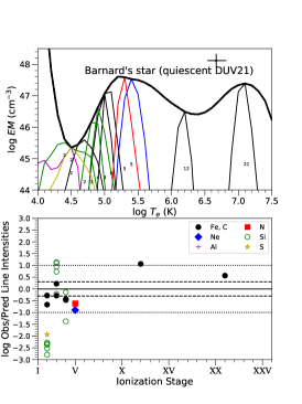
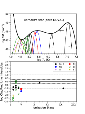
where (K) = 0.1 is the temperature resolution of the ATOMDB models used in our work. Once the DEMs were transformed into EMDs (Fig. 6), we calculated the predicted line fluxes using the solar coronal abundances assumed in LO17 and DUV21 to test how good are the models provided by those authors. The results of this comparison are shown in Fig. 7.
The smooth shape imposed by polynomial fits yields large differences with our results, in special in the temperature ranges with fewer spectral lines, such as the regions with (K)4.5, and 5.2–6.0. DUV21 used solar coronal abundances in all cases, which might explain some of the discrepancies, as acknowledged by DUV21. While this assumption could be a good approximation for a solar-like quiet corona, like that of HD 209458, it is inadequate for a very active star like AU Mic111111DUV21 DEM was based on a different dataset from ours., as shown in Fig. 7 (see e.g., Sanz-Forcada et al., 2003b). In the case of Barnard’s star, DUV21 made a different DEM for flaring and quiescent stages, while we used only one overall EMD. However none of the DUV21 functions match the minimum of the EMD as sampled by us. Finally, TRAPPIST-1 model also over-interprets the information available in the X-rays spectra by providing a continuous DEM along the high temperature range. In all cases, there are obvious discrepancies, of up to three orders of magnitude, between predicted and observed line fluxes when the EMDs of DUV21 and LOU17 are employed. Their EUV broadband fluxes differ by up to 1 dex from ours (Table ).
| Reference | AU Mic | TRAPPIST-1 | Barnard’s Star | Barnard’s Star | HD 209458 |
|---|---|---|---|---|---|
| (quiescence) | (flare) | ||||
| DUV21, LOU17 | 28.93 | 27.33 | 25.71 | 26.61 | 28.20 |
| This work | 29.39 | 26.29 | 26.13 | 28.45 | |
A.2 Comparison with other scaling laws
In this section, we compare the results from our scaling law described in Sect. 4.2 and other works in the literature. Our X-ray vs. EUVH luminosity linear fit has an RMS=0.406. Figure 8 includes a comparison with the SF11 linear fit (RMS=0.411 with the current dataset) to and . The addition of UV high-spectral resolution data and values with larger X-ray luminosity seems to lower the EUV modeled luminosity, but both fits are consistent.
Scaling laws based on the surface stellar flux are shown in Fig. 9 together with our own fit to the data. Our fit is
| (9) |
where , all in c.g.s units. The plot includes only the stars of our sample with a stellar radius available in the Extrasolar Planet Encyclopaedia131313https://exoplanet.eu database, 65 stars. Our linear fit to the data shows a Pearson’s correlation factor , and an RMS of 0.386. The Johnstone et al. (2021) relation has an RMS of 0.405 with this dataset, Chadney et al. (2015) an RMS=0.445, and King et al. (2018) an RMS=0.462. The literature fits have a worse RMS than our linear fit between and (Fig. 3). They also have a dependence on the stellar radius, introducing a new source of uncertainty. We display the literature fits extrapolated to cover our range of values. Although all of the fits are roughly consistent with ours, discrepancies arise for the most active stars, and especially for the least active stars.
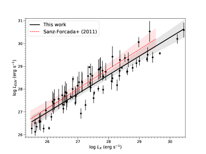
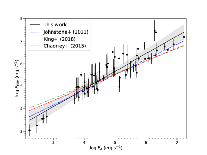
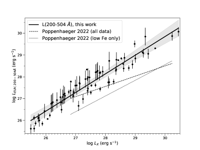
Poppenhaeger (2022) calculated the EUV flux in the range 200–504 Å based on EUVE observations in a number of targets. This is a spectral range severely affected by ISM absorption (see, e.g., Sanz-Forcada et al., 2003a) and the spectra are contaminated by geocoronal emission around the He ii 304 Å line, as those in Johnstone et al. (2021). Since Poppenhaeger (2022) calculated the absorption based on two lines that are absent in most of the spectra, there may be systematic under- or over-estimation in this calculation. Moreover, most lines above are absent in EUVE spectra, and some of the observed lines are actually the second order of stronger bluewards lines. An example is the EUVE spectrum of AD Leo (Sanz-Forcada & Micela, 2002), a star at only 5 pc from us. The low quality spectrum of AD Leo shown in Fig. 9 of Poppenhaeger (2022) came from an automatic reduction available in HEASARC, quite below the quality level that can be achieved by a customized data reduction, which would anyway be insufficient to accurately calculate the flux in the 200–504 Å spectral range. In Fig. 10 we show the fit that we did to our calculated EUV fluxes in this range, as compared with the Poppenhaeger (2022) fits (their relation was also applied by Fossati et al., 2023). They are obviously discrepant. Our linear fit is
| (10) |
where in c.g.s. units. This is valid in the range . This fit has a Pearson’s correlation factor and an RMS=0.326. The spectral range used to calculate by Poppenhaeger (2022) was 0.2–5 keV, instead of our 0.12–2.4 keV range. We tested the impact of this difference by measuring the flux in an active (AD Leo) star and a more quiet (GJ 357) star. The flux in the 0.2–5 keV range is 4% lower for AD Leo, and dex lower for GJ 357, thus increasing the differences between the two relations.
Appendix B Relations between He i 10830 Å equivalent width and XUV flux
In this section, we seek an empirical relationship between the stellar XUV irradiation, measured in the 5–504 Å range, and the equivalent width () of the He i 10830 Å line in the planet atmosphere. The equivalent width, , of an absorbing line over the frequency interval in a planetary atmosphere during the primary transit is given by
| (11) |
where is the frequency, is the absorption of the entire planetary atmosphere, is the stellar radius, and we assume that . The absorption is obtained by integrating the partial absorption of the areas covered by infinitesimal spherical rings over all impact parameter values (see, e.g., Sect. 3.3 in Lampón et al. 2020 and Fig. 11) as:
| (12) |
where we assume spherical symmetry, is the radius of the planet, TOA is the top of the atmosphere in front of the star, and the transmission is given by
| (13) |
where is the absorption coefficient (also denoted by , the absorption cross section) of the He(23S) lines and is the He(23S) concentration.
To estimate the dependence of on the different parameters, we considered the two extreme conditions of (a) optically thick, where the transmission near the line center, , is close to zero, and (b) optically thin, where is close to unity. This approach in two extreme situations seems reasonable as we know that most gas giant atmospheres have, in general, a narrow (compressed) region at low altitudes with large He(23S) concentrations, and an extended and slowly decreasing He(23S) concentration at medium to larger radii (see, e.g., Fig. A.1 in Lampón et al. 2023). The first region can be considered in optically thick conditions while the latter in the optically thin regime.
B.1 Optically thick
In this case, , the is given by that produced by an opaque ring of height . From Eqs. 11 and 12, with , we obtain
| (14) |
To estimate the extension of the opaque region, , it is reasonable to assume that it is proportional to the irradiating XUV flux , as this flux controls the He(23S) concentration that enters into Eq. 13. In fact, the planets with larger XUV fluxes have larger peaks of He(23S) concentrations (see Fig. A.1 in Lampón et al. 2023). In addition, for a planet with a stronger gravitational potential, , it is expected that its atmosphere (and the He(23S) concentration) is more compressed and hence should be smaller. It is then reasonable that in this optically thick limit we have
| (15) |
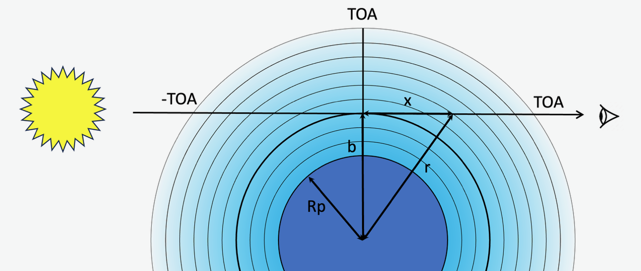
B.2 Optically thin
In this case the transmission over the interval can be approximated by
| (16) |
where is the column density along the line of sight at impact parameter (see Fig. 11) and we have assumed that the absorption coefficient does not depend on . Assuming spherical symmetry and changing the integration variable to , the distance from the center of the planet, e.g., and , we obtain
| (17) |
To further evaluate and the let us make some assumptions on . The He(23S) concentration can be well approximated by
| (18) |
where the exponent usually takes values between 2 and 5 and is the He(23S) concentration at (see, e.g., Fig. A.1(c) in Lampón et al., 2023). Note that the He(23S) peak concentration, , usually occurs very close to the lower boundary of the atmosphere; hence . Then, we obtain
| (19) |
and, by performing the integral, we obtain
| (20) |
valid for , which is amply met in our case.
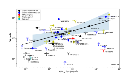
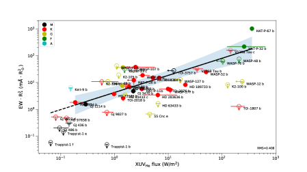
Including this expression into Eq. 16, and considering Eqs. 11 and 12, we obtain
| (21) |
Performing the integral in Eq. 21 and considering that , we find that the integral is independent of for , it is proportional to for = 3, and is proportional to for . Hence, as the functions are constants,
| (22) |
where we also considered that and the is, as in the case of the optically thick, proportional to . Then, for a given planet with an He(23S) concentration profile with a slope as in Eq. 18, the in the optically thin limit would be proportional to with ranging from 1 to 3. For the optically thick limit we obtain a dependence directly proportional to . Hence, overall, we expect a dependence of of the form of
| (23) |
with varying between 1 and 3 depending on the specific conditions of the planets.
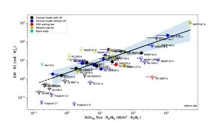
We probed the dependence on the stellar area in Fig. 13, with a substantial improvement with respect to Fig. 12. If we consider the relation between and we get a Pearson’s correlation factor of . For the relation between and we get a correlation factor of , and for that against we reach (Fig. 14). Finally, a dependence on results in a further improvement (Fig. 4, ). Table shows the and RMS of the fits with different exponents of . If we use against as in Zhang et al. (2023a) assuming that =, our data improve their log-log fit, with a correlation coefficient of , but it is still worse than the fit using .
| RMS | |||||
|---|---|---|---|---|---|
| 1 | 0.891 | 0.298 | 1.18 | ||
| 1.5 | 0.899 | 0.287 | 1.07 | ||
| 2 | 0.898 | 0.289 | 0.96 | ||
| 2.5 | 0.893 | 0.295 | 0.86 | ||
| 3 | 0.886 | 0.304 | 0.75 |
Appendix C Main tables
| Star name | SpT | (J2000.0) | (J2000.0) | Date | Instr.aaaaXMM-Newton or Chandra instrument used to measure the X-ray flux. EPIC exposure time is the average of all EPIC detectors. S/N is the signal-to-noise ratio of the summed observations of the same star. | t (ks) | S/N |
| New XMM-Newton observations | |||||||
| WASP-76 | F7IV-V | 01:46:31.9 | :42:02 | 2020-01-01 | EPIC | 9.0 | 1.2 |
| HAT-P-32A | F8V: | 02:04:10.5 | :41:15 | 2019-08-30 | EPIC | 15.3 | 11.3 |
| KELT-7 | F3IV-V | 05:13:11.1 | :19:05 | 2019-08-29 | EPIC | 7.2 | 11.7 |
| WASP-12 | G0V | 06:30:32.8 | :40:20 | 2019-09-14 | EPIC | 8.8 | 1.3 |
| WASP-13 | G1V-IV | 09:20:24.7 | :52:56 | 2019-10-18 | EPIC | 8.9 | 3.2 |
| WASP-127 | G5V | 10:42:14.7 | :50:06 | 2019-11-24 | EPIC | 5.9 | 0.4 |
| WASP-107 | K7V | 12:33:32.7 | :08:46 | 2018-06-22 | EPIC | 57.5 | 16.7 |
| HAT-P-12 | K4V | 13:57:33.1 | :29:35 | 2019-11-25 | EPIC | 7.4 | 2.2 |
| WASP-39 | G9V | 14:29:18.2 | :26:40 | 2020-02-08 | EPIC | 13.4 | 1.5 |
| KELT-8 | G2V-IV | 18:53:13.3 | :07:37 | 2019-09-14 | EPIC | 7.8 | 1.1 |
| GJ 806 | M1.5V | 20:45:04.1 | :29:57 | 2023-12-07 | EPIC | 17.5 | 6.9 |
| HD 201585 | A8V | 21:10:12.4 | :44:21 | 2019-10-29 | EPIC | 5.7 | 2.4 |
| HAT-P-1 | G0V | 22:57:46.9 | :40:29 | 2019-12-02 | EPIC | 16.8 | 2.1 |
| Other objects from XMM-Newton and Chandra archives | |||||||
| GJ 12 | M3.0V | 00:15:49.2 | :33:22 | 2018-06-16 | EPIC | 17.8 | 4.5 |
| WASP-77A | G8V | 02:28:37.2 | :03:39 | 2013-11-09 | ACIS | 9.9 | 3.7 |
| Teegarden’s star | M7.0V | 02:53:00.9 | :52:53 | 2021-08-03 | EPIC | 29.1 | 27.3 |
| HD 283636 | K0V | 04:23:55.1 | :49:21 | 2021-08-23 | EPIC | 4.8 | 8.1 |
| K2-136 | K5V | 04:29:39.0 | :52:58 | 2018-09-11 | EPIC | 37.2 | 21.9 |
| HD 63433 | G5V | 07:49:55.1 | :21:47 | 2021-03-26 | EPIC | 4.5 | 57.4 |
| GJ 3470 | M1.5V | 07:59:05.8 | :23:29 | 2015-04-15 | EPIC | 15.2 | 18.0 |
| K2-100 | G0V | 08:38:24.3 | :06:22 | 2013-10-30 | EPIC | 66.3 | 34.6 |
| K2-100 | 2015-05-05 | EPIC | 54.0 | … | |||
| HD 73583 | K4V | 08:38:45.3 | :15:24 | 2021-04-21 | EPIC | 9.4 | 19.2 |
| GJ 357 | M2.5V | 09:36:01.6 | :39:39 | 2019-05-19 | EPIC | 29.1 | 7.5 |
| AD Leo | M3.0V | 10:19:36.3 | :52:12 | 2000-01-22 | LETG | 10 | 168 |
| AD Leo | 2000-10-24 | LETG | 48 | … | |||
| AD Leo | 2002-06-01 | HETG | 46 | 112 | |||
| Lalande 21185 | M1.5V | 11:03:20.2 | :58:12 | 2001-05-15 | RGS | 19.7 | 60.3 |
| Lalande 21185 | 2004-05-12 | RGS | 44.3 | … | |||
| HD 97658 | K1V | 11:14:33.2 | :42:37 | 2015-06-04 | EPIC | 29.9 | 16.6 |
| GJ 486 | M3.5V | 12:47:56.6 | :45:05 | 2021-12-23 | EPIC | 31.5 | 10.3 |
| Proxima Cen | M5.5V | 14:29:42.9 | :40:46 | 2001–2018 | RGS | 506 | 360 |
| TOI-836 | K7V | 15:00:19.4 | :27:15 | 2022-07-25 | EPIC | 10.1 | 7.2 |
| HD 149026 | G0V | 16:30:29.6 | :20:50 | 2015-08-14 | EPIC | 17.1 | 6.0 |
| GJ 1214 | M4.5V | 17:15:18.9 | :57:50 | 2013-09-27 | EPIC | 31.7 | 4.3 |
| Barnard’s star | M3.5V | 17:57:48.5 | :41:36 | 2019-06-17 | ACIS | 26.7 | 11.4 |
| TOI-2134 | K5V | 18:07:44.4 | :04:27 | 2022-09-12 | EPIC | 17.7 | 5.7 |
| HAT-P-11 | K4V | 19:50:50.2 | :04:51 | 2015-05-19 | EPIC | 25.0 | 13.4 |
| HD 235088 | K2V | 20:02:27.4 | :22:37 | 2021-07-07 | EPIC | 11.4 | 26.6 |
| WASP-80 | K7V | 20:12:40.2 | :08:39 | 2014-05-15 | EPIC | 15.3 | 15.6 |
| WASP-80 | 2015-05-13 | EPIC | 29.2 | … | |||
| KELT-9 | A0V | 20:31:26.4 | :56:20 | 2017-11-09 | EPIC | 50.0 | 2.4 |
| AU Mic | M0.5V | 20:45:09.5 | :20:27 | 2000-10-13 | RGS | 52.7 | 670 |
| WASP-69 | K4V | 21:00:06.2 | :05:40 | 2016-10-21 | EPIC | 27.4 | 30.6 |
| TRAPPIST-1 | M8.0V | 23:06:29.4 | :02:29 | 2014-12-17 | EPIC | 27.2 | 19.0 |
| TRAPPIST-1 | 2017-11-23 | EPIC | 49.8 | … | |||
| TRAPPIST-1 | 2017-11-29 | EPIC | 39.8 | … | |||
| TRAPPIST-1 | 2017-12-12 | EPIC | 35.3 | … | |||
| TRAPPIST-1 | 2018-12-10 | EPIC | 15.6 | … | |||
| WASP-52 | K2V | 23:13:58.8 | :45:41 | 2014-01-03 | ACIS | 9.8 | 3.5 |
| GJ 9827 | K6V | 23:27:04.8 | :17:11 | 2018-05-27 | EPIC | 19.0 | 8.7 |
| GJ 9827 | 2018-06-23 | EPIC | 14.1 | … | |||
| GJ 9827 | 2018-11-27 | EPIC | 11.3 | … | |||
| New archival data of X-exoplanets objects included in this work | |||||||
| And | F8V | 01:36:47.8 | :24:20 | 2013-08-04 | EPIC | 16.7 | 49.4 |
| HD 27442 | K2IV | 04:16:29.0 | :18:08 | 2009-02-10 | EPIC | 7.50 | 16.6 |
| HD 27442 | 2016-09-30 | EPIC | 35.7 | … | |||
| HD 75289 | G0V | 08:47:40.4 | :44:12 | 2005-04-28 | EPIC | 8.14 | 3.5 |
| HD 75289 | 2013-11-27 | EPIC | 15.1 | … | |||
| GJ 436 | M2.5V | 11:42:11.1 | :42:24 | 2008-12-10 | EPIC | 30.3 | 21.7 |
| GJ 436 | 2015-11-21 | EPIC | 22.5 | … | |||
| HD 108147 | F9V | 12:25:46.3 | :01:20 | 2002-08-10 | EPIC | 5.74 | 35.8 |
| HD 108147 | 2010-08-08 | EPIC | 52.5 | … | |||
| GJ 674 | M2.5V | 17:28:39.9 | :53:43 | 2008-09-05 | EPIC | 20.0 | 223 |
| GJ 674 | 2018-04-03 | EPIC | 24.5 | … | |||
| HD 189733 | K2V | 20:00:43.7 | :42:39 | 2007-04-17 | EPIC | 38.2 | 460 |
| HD 189733 | 2009-05-18 | EPIC | 30.1 | … | |||
| HD 189733 | 2011-04-30 | EPIC | 28.1 | … | |||
| HD 189733 | 2012-05-08 | EPIC | 56.9 | … | |||
| HD 189733 | 2013-05-09 | EPIC | 29.3 | … | |||
| HD 189733 | 2013-11-03 | EPIC | 28.0 | … | |||
| HD 189733 | 2014-04-05 | EPIC | 26.7 | … | |||
| HD 189733 | 2014-10-18 | EPIC | 26.1 | … | |||
| HD 189733 | 2014-11-08 | EPIC | 25.6 | … | |||
| HD 189733 | 2015-04-03 | EPIC | 28.8 | … | |||
| HD 190360 | G6IV | 20:03:37.4 | :53:48 | 2005-04-25 | EPIC | 4.21 | 3.0 |
| HD 190360 | 2005-11-18 | EPIC | 3.64 | … | |||
| GJ 832 | M1.5V | 21:33:34.0 | :00:32 | 2014-10-11 | EPIC | 10.2 | 17.6 |
| Star name | Date | Instrument | |
|---|---|---|---|
| 55 Cnc | 2016-04-04–2017-02-14 | COS/G130M | |
| AD Leo | 2000-03-10, 2002-06-01 | STIS/E140M | |
| AD Leo | 1993–2000 | EUVEaaaaFluxes from Sanz-Forcada & Micela (2002). | |
| AU Mic | 1998-09-06, 2020-07-02 | STIS/E140M | |
| AU Mic | 2000-08-26, 2001-10-10 | FUSE | |
| AU Mic | 1993–1996 | EUVE | |
| Barnard’s star | 2019-03-04 | COS/G130M+STIS/G140LbbbbSTIS fluxes were corrected to match the level of the mean of the fluxes of the C iii 1176 Å, Si iii 1206 Å, and C ii 1335 lines in the COS spectrum. | |
| GJ 357 | 2021-04-21 | COS/G130M+G160M | |
| GJ 436 | 2012-06-23, 2015-06-25 | COS/G130M+G160M | |
| GJ 486 | 2022-03-15 | STIS/G140L+G140M | |
| GJ 674 | 2018-04-02 | COS/G130M+STIS/G140L | |
| GJ 1214 | 2012-08-04, 2015-08-20 | COS/G130M+G160M | |
| GJ 3470 | 2017-12-27–2018-12-23 | COS/G130M | |
| GJ 9827 | 2018-08-23–2020-10-10 | STIS/G140M | |
| HD 63443 | 2020-10-29–2022-02-17 | STIS/G140M | |
| HD 73583 | 2021-12-24–2023-03-02 | STIS/G140M | |
| HD 97658 | 2015-02-13 | COS/G130M+G160M | |
| HD 149026 | 2021-07-26, 2022-10-05 | STIS/G140L | |
| HD 189733 | 2009-0916–2017-07-03 | COS/G130MccccSummed spectrum from HSLA (Hubble Spectroscopic Legacy Archive), available at https://archive.stsci.edu/hst/spectral_legacy/. | |
| HD 209458 | 2009-09-15 | COS/G130M+G160MddddFluxes from France et al. (2010). | |
| Lalande 21185 | 2020-01-14 | STIS/E140M | |
| Proxima Cen | 2019-04-28–2019-07-01 | STIS/E140M | |
| Proxima Cen | 2003-04-05 | FUSE | |
| Proxima Cen | 1993-05-21 | EUVE | |
| Boo | 1999-06-09, 1999-06-26 | STIS/G140M | |
| TOI-836 | 2022-07-28 | STIS/G140M+G140L | |
| TRAPPIST-1 | 2016-09-26–2019-06-07 | COS/G130M+G160M | |
| And | 2011-11-09 | STIS/E140M | |
| WASP-13 | 2015-04-21 | COS/G140L | |
| WASP-52 | 2021-10-05, 2021-10-07 | STIS/G140M+G140L | |
| WASP-77A | 2022-02-02 | STIS/G140L |
| Planet name | SpT | Stellar distance | |||||||||
|---|---|---|---|---|---|---|---|---|---|---|---|
| (pc) | (erg s-1) | (erg s-1) | (erg s-1) | (erg s-1) | (MJ) | (au) | (erg s-1cm-2) | (g2s-1cm-3)bbbb1 MJ Gyr-1= g s-1, 1 M⊕ Gyr-1= g s-1. Mass loss rates based on upper limits are expressed in parenthesis. | |||
| 14 Her b | K0V | 17.8990.010 | 33.41 | 26.92 | 27.70 | 27.16 | 5.215 | 2.820 | 0.58 | 0.99 | 2.9e+06 |
| 14 Her c | 7.031 | 27.000 | 2.55 | 2.96 | 3.2e+04 | ||||||
| 16 Cyg B b | G2V | 21.1280.009 | 33.68 | 26.78 | 27.98 | 27.45 | 1.640 | 1.680 | ¡ 0.11 | ¡-0.36 | (1.4e+07) |
| 2M1207 A b | M8V | 64.680.50 | 31.08 | 26.16 | 27.36 | 26.83 | 5.500 | 42.000 | ¡-3.29 | ¡-3.78 | (5.8e+03) |
| 30 Ari B bccccControversial or retracted planet detection. | F6V | 44.9240.061 | 34.20 | 29.67 | 29.57 | 29.51 | 9.880 | 0.995 | 2.47 | 2.45 | 3.3e+09 |
| 47 Uma b | G0V | 13.8870.019 | 33.78 | 25.75 | 26.62 | 26.26 | 2.530 | 2.100 | 1.42 | 1.71 | 4.2e+05 |
| 47 Uma c | 0.540 | 3.600 | 1.89 | 2.18 | 1.4e+05 | ||||||
| 47 Uma d | 1.640 | 11.600 | 2.91 | 3.20 | 1.4e+04 | ||||||
| 51 Peg b | G2IV | 15.5280.019 | 33.79 | 26.66 | 27.86 | 27.33 | 0.460 | 0.052 | ¡ 3.01 | ¡ 2.54 | (1.1e+10) |
| 55 Cnc b | G8V | 12.5870.006 | 33.38 | 26.77 | 27.67 | 27.39 | 0.840 | 0.113 | 2.17 | 1.92 | 1.6e+09 |
| 55 Cnc c | 0.178 | 0.237 | 1.52 | 1.28 | 3.8e+08 | ||||||
| 55 Cnc d | 3.840 | 5.446 | 1.20 | 1.44 | 7.1e+05 | ||||||
| 55 Cnc e | 0.027 | 0.015 | 3.90 | 3.66 | 8.9e+10 | ||||||
| 55 Cnc f | 0.148 | 0.773 | 0.50 | 0.26 | 3.5e+07 | ||||||
| AD Leo bccccControversial or retracted planet detection. | M3.0V | 4.9650.001 | 31.96 | 28.61 | 28.77 | 28.54 | 0.073 | 0.025 | 4.75 | 4.64 | 6.4e+11 |
| AU Mic b | M1.5V | 9.7140.002 | 32.58 | 29.44 | 29.39 | 29.25 | 0.028 | 0.070 | 4.58 | 4.51 | 4.2e+11 |
| AU Mic c | 0.0456 | 0.149 | 4.12 | 4.05 | 1.5e+11 | ||||||
| AU Mic d | 0.0032 | 0.085 | 4.41 | 4.35 | 2.9e+11 | ||||||
| Barnard’s star b | M3.5V | 1.8280.0001 | 31.15 | 25.61 | 26.13 | 25.74 | 0.0012 | 0.0229 | 2.07 | 1.81 | 1.3e+09 |
| CoRoT-7 b | K0V | 159.490.25 | 33.27 | 28.98 | 30.06 | 29.84 | 0.019 | 0.017 | 6.16 | 5.98 | 1.6e+13 |
| CoRoT-7 c | 0.042 | 0.046 | 5.30 | 5.13 | 2.3e+12 | ||||||
| CoRoT-7 d | 17.142 | 0.080 | 4.82 | 4.65 | 7.4e+11 | ||||||
| GJ 12 b | M3.0V | 12.1670.004 | 31.46 | 25.78 | 26.58 | 26.05 | 0.0049 | 0.066 | 1.55 | 1.15 | 4.0e+08 |
| GJ 86 b | K1V | 10.7610.006 | 33.18 | 27.41 | 28.13 | 28.44 | 4.270 | 0.118 | 3.10 | 2.52 | (1.4e+10) |
| GJ 317 b | M3V | 15.1790.009 | 31.93 | 26.59 | 27.87 | 27.21 | 1.753 | 1.151 | 0.32 | 0.27 | 2.4e+07 |
| GJ 317 c | 1.644 | 5.230 | 0.99 | 1.59 | 1.1e+06 | ||||||
| GJ 357 b | M2.5V | 9.4360.002 | 31.78 | 25.66 | 26.36 | 25.93 | 0.0066 | 0.033 | 1.95 | 1.63 | 1.0e+09 |
| GJ 357 c | 0.012 | 0.061 | 1.42 | 1.10 | 2.9e+08 | ||||||
| GJ 357 d | 0.023 | 0.204 | 0.37 | 0.05 | 2.6e+07 | ||||||
| GJ 436 b | M2.5V | 9.7750.003 | 31.97 | 26.14 | 26.79 | 26.30 | 0.067 | 0.029 | 2.50 | 2.16 | 3.6e+09 |
| GJ 486 b | M3.5V | 8.0790.002 | 31.66 | 25.50 | 26.27 | 25.69 | 0.0089 | 0.017 | 2.41 | 1.98 | 2.9e+09 |
| GJ 674 b | M2.5V | 4.5530.001 | 31.79 | 27.67 | 28.02 | 27.76 | 0.040 | 0.039 | 3.55 | 3.39 | 3.9e+10 |
| GJ 806 b | M1.5V | 12.0640.003 | 32.01 | 26.23 | 27.53 | 26.87 | 0.0060 | 0.014 | 3.81 | 3.21 | 7.2e+10 |
| GJ 806 c | 0.018 | 0.052 | 2.67 | 2.07 | 5.2e+09 | ||||||
| GJ 832 b | M1.5V | 4.96710.0006 | 32.04 | 26.18 | 27.45 | 26.80 | 0.740 | 3.600 | 1.09 | 1.67 | 9.1e+05 |
| GJ 876 b | M4V | 4.6720.001 | 31.69 | 26.20 | 27.37 | 26.83 | 3.534 | 0.214 | 1.29 | 0.81 | 2.2e+08 |
| GJ 876 c | 0.698 | 0.134 | 1.70 | 1.22 | 5.6e+08 | ||||||
| GJ 876 d | 0.019 | 0.021 | 3.31 | 2.83 | 2.3e+10 | ||||||
| GJ 876 e | 0.042 | 0.345 | 0.88 | 0.39 | 8.5e+07 | ||||||
| GJ 1214 b | M4.5V | 14.6410.015 | 31.13 | 25.88 | 26.27 | 25.94 | 0.026 | 0.014 | 2.67 | 2.47 | 5.3e+09 |
| GJ 3470 b | M1.5V | 29.3940.026 | 32.19 | 27.53 | 27.84 | 27.66 | 0.040 | 0.036 | 3.46 | 3.35 | 3.2e+10 |
| GJ 9827 b | K6V | 29.6560.018 | 32.61 | 26.53 | 27.14 | 26.57 | 0.015 | 0.019 | 3.25 | 2.86 | 2.0e+10 |
| GJ 9827 c | 0.0060 | 0.039 | 2.61 | 2.22 | 4.5e+09 | ||||||
| GJ 9827 d | 0.011 | 0.056 | 2.30 | 1.91 | 2.2e+09 | ||||||
| GQ Lup b | K7V | 154.080.71 | 33.69 | 30.45 | 30.59 | 30.17 | 31.000 | 32.000 | 0.17 | 0.17 | 1.7e+07 |
| HAT-P-1 b | G0V | 160.260.26 | 33.79 | 28.17 | 29.34 | 28.90 | 0.523 | 0.056 | ¡ 4.40 | ¡ 4.03 | (2.8e+11) |
| HAT-P-11 b | K4V | 37.8360.014 | 33.01 | 27.38 | 28.96 | 28.37 | 0.074 | 0.053 | 4.08 | 3.51 | 1.3e+11 |
| HAT-P-11 c | 1.595 | 4.130 | 0.29 | 0.27 | 2.2e+07 | ||||||
| HAT-P-12 b | K4V | 142.050.20 | 32.88 | 27.95 | 29.16 | 28.62 | 0.210 | 0.038 | ¡ 4.56 | ¡ 4.09 | (4.1e+11) |
| HAT-P-32 b | F8V | 286.51.6 | 33.90 | 29.34 | 30.53 | 29.88 | 0.750 | 0.034 | 6.02 | 5.47 | 1.2e+13 |
| HD 4308 b | G5V | 22.0460.010 | 33.59 | 26.15 | 27.35 | 26.82 | 0.041 | 0.118 | ¡ 1.78 | ¡ 1.31 | (6.8e+08) |
| HD 20367 b | G0V | 26.0550.020 | 33.77 | 29.27 | 29.51 | 29.18 | 1.070 | 1.250 | 2.06 | 1.89 | 1.3e+09 |
| HD 27442 A b | K2IV | 18.4400.034 | 34.88 | 26.64 | 27.47 | 27.21 | 1.350 | 1.160 | 0.05 | 0.26 | 1.0e+07 |
| HD 46375 A b | K1IV | 29.5160.017 | 33.40 | 27.03 | 28.30 | 27.64 | 0.230 | 0.041 | 3.65 | 3.06 | 5.0e+10 |
| HD 49674 b | G5V | 42.8820.037 | 33.55 | 27.47 | 28.58 | 28.01 | 0.100 | 0.058 | 3.64 | 3.14 | 4.9e+10 |
| HD 50554 b | F8V | 31.0660.019 | 33.74 | 26.36 | 27.54 | 27.07 | 5.160 | 2.410 | ¡-0.64 | ¡-1.07 | (2.6e+06) |
| HD 52265 b | G0V | 29.9220.018 | 33.94 | 26.99 | 28.15 | 27.63 | 1.210 | 0.520 | 1.30 | 0.84 | 2.2e+08 |
| HD 63433 b | G5V | 22.3810.010 | 33.46 | 28.78 | 28.93 | 28.52 | 0.068 | 0.072 | 4.00 | 3.81 | 1.1e+11 |
| HD 63433 c | 0.048 | 0.146 | 3.39 | 3.20 | 2.8e+10 | ||||||
| Planet name | SpT | Stellar distance | |||||||||
|---|---|---|---|---|---|---|---|---|---|---|---|
| (pc) | (erg s-1) | (erg s-1) | (erg s-1) | (erg s-1) | (MJ) | (au) | (erg s-1cm-2) | (g2s-1cm-3)bbbb1 MJ Gyr-1= g s-1, 1 M⊕ Gyr-1= g s-1. Mass loss rates based on upper limits are expressed in parenthesis. | |||
| HD 63433 d | … | 0.050 | 4.31 | 4.12 | 2.3e+11 | ||||||
| HD 70642 b | G5IV | 29.2830.017 | 33.40 | 26.37 | 27.57 | 26.96 | 2.000 | 3.300 | 0.89 | 1.42 | 1.5e+06 |
| HD 73583 b | K4V | 31.5860.020 | 32.83 | 27.82 | 27.98 | 27.54 | 0.032 | 0.060 | 3.19 | 3.00 | 1.8e+10 |
| HD 73583 c | 0.030 | 0.123 | 2.57 | 2.38 | 4.2e+09 | ||||||
| HD 75289 b | G0V | 29.0280.017 | 33.88 | 25.60 | 26.52 | 26.34 | 0.470 | 0.046 | 1.79 | 1.64 | 6.9e+08 |
| HD 93083 b | K3V | 28.4820.016 | 33.18 | 26.83 | 28.01 | 27.40 | 0.370 | 0.477 | 1.23 | 0.70 | 1.9e+08 |
| HD 95089 b | K0IV | 135.500.37 | 34.71 | 26.60 | 27.80 | 27.27 | 1.200 | 1.510 | ¡ 0.01 | 0.45 | (1.1e+07) |
| HD 95089 c | 3.970 | 3.447 | 0.71 | 1.17 | (2.2e+06) | ||||||
| HD 97658 b | K1V | 21.5610.009 | 33.13 | 26.92 | 27.39 | 27.17 | 0.025 | 0.080 | 2.26 | 2.11 | 2.1e+09 |
| HD 99492 b | K2V | 18.1620.010 | 33.11 | 26.57 | 27.70 | 27.11 | 0.080 | 0.123 | 2.10 | 1.59 | 1.4e+09 |
| HD 99492 c | 0.056 | 5.400 | 1.18 | 1.69 | 7.4e+05 | ||||||
| HD 101930 b | K1V | 29.9580.018 | 33.24 | 26.00 | 27.20 | 26.67 | 0.300 | 0.302 | ¡ 0.93 | ¡ 0.35 | (9.5e+07) |
| HD 102195 b | K0V | 29.3600.017 | 33.26 | 28.37 | 29.28 | 28.82 | 0.490 | 0.049 | 4.50 | 4.12 | 3.6e+11 |
| HD 108147 b | F9V | 38.8200.030 | 33.87 | 27.91 | 28.76 | 28.29 | 0.261 | 0.102 | 3.35 | 2.97 | 2.5e+10 |
| HD 111232 b | G8V | 28.8930.017 | 33.41 | 26.50 | 27.71 | 27.18 | 6.800 | 1.970 | 0.31 | 0.77 | (5.5e+06) |
| HD 114386 b | K3V | 27.9800.016 | 33.03 | 26.63 | 27.43 | 27.02 | 1.240 | 1.020 | 0.02 | 0.29 | 1.2e+07 |
| HD 114386 c | 1.190 | 1.832 | 0.49 | 0.80 | 3.7e+06 | ||||||
| HD 114762 b | F9V | 38.170.16 | 33.75 | 26.71 | 27.91 | 27.38 | 10.980 | 0.353 | ¡ 1.39 | ¡ 0.92 | (2.8e+08) |
| HD 114783 b | K0V | 21.0300.013 | 33.19 | 26.52 | 27.32 | 26.88 | 1.100 | 1.160 | 0.19 | 0.54 | 7.2e+06 |
| HD 114783 c | 0.610 | 5.047 | 1.47 | 1.82 | 3.8e+05 | ||||||
| HD 130322 b | K0V | 31.9080.031 | 33.33 | 27.33 | 28.57 | 27.93 | 1.020 | 0.090 | 3.24 | 2.67 | 1.9e+10 |
| HD 149026 b | G0V | 76.220.12 | 34.00 | 27.40 | 28.10 | 27.44 | 0.356 | 0.043 | 3.46 | 3.01 | 3.3e+10 |
| HD 154345 b | G8V | 18.2680.007 | 33.35 | 27.13 | 28.34 | 27.75 | 1.000 | 4.300 | 0.35 | 0.87 | 5.0e+06 |
| HD 164922 b | K0V | 21.9780.010 | 33.43 | 25.51 | 26.69 | 26.22 | 0.365 | 2.160 | 1.40 | 1.82 | (4.5e+05) |
| HD 164922 c | 0.041 | 0.341 | ¡ 0.21 | 0.22 | (1.8e+07) | ||||||
| HD 164922 d | 0.033 | 0.123 | ¡ 1.09 | ¡ 0.67 | (1.4e+08) | ||||||
| HD 164922 e | 0.033 | 0.229 | ¡ 0.55 | ¡ 0.13 | (4.0e+07) | ||||||
| HD 179949 b | F8V | 27.5410.030 | 33.88 | 28.64 | 29.29 | 28.98 | 0.920 | 0.045 | 4.62 | 4.39 | 4.7e+11 |
| HD 187123 b | G2V | 46.0410.042 | 33.70 | 27.28 | 28.46 | 27.99 | 0.520 | 0.043 | ¡ 3.78 | ¡ 3.36 | (6.8e+10) |
| HD 187123 c | 1.990 | 4.890 | 0.34 | 0.76 | (5.2e+06) | ||||||
| HD 189733 b | K2V | 19.7750.008 | 33.10 | 28.36 | 28.81 | 28.53 | 1.154 | 0.031 | 4.51 | 4.32 | 3.6e+11 |
| HD 190360 b | G6IV | 16.0030.010 | 33.69 | 26.54 | 27.72 | 27.25 | 1.495 | 3.920 | 0.88 | 1.31 | (1.5e+06) |
| HD 190360 c | 0.064 | 0.128 | ¡ 2.09 | ¡ 1.66 | (1.4e+09) | ||||||
| HD 195019 b | G3IV | 37.5230.028 | 33.87 | 26.34 | 27.51 | 27.04 | 3.700 | 0.139 | ¡ 1.81 | ¡ 1.38 | (7.2e+08) |
| HD 201585 b | A8V | 182.150.66 | 34.68 | 28.62 | 29.80 | 29.33 | 3.695 | 0.043 | ¡ 5.10 | ¡ 4.69 | (1.4e+12) |
| HD 209458 b | G0V | 48.1460.070 | 33.80 | 26.84 | 28.45 | 27.92 | 0.685 | 0.047 | 3.66 | 3.15 | 5.1e+10 |
| HD 216435 b | K6V | 33.1240.033 | 34.13 | 27.74 | 28.95 | 28.30 | 1.260 | 2.560 | 0.71 | 0.14 | 5.8e+07 |
| HD 216437 b | G4IV | 26.6950.021 | 33.62 | 26.63 | 27.83 | 27.27 | 1.820 | 2.320 | 0.32 | 0.82 | 5.3e+06 |
| HD 217107 b | G8IV | 20.0880.012 | 33.62 | 25.76 | 26.93 | 26.46 | 1.394 | 0.075 | ¡ 1.77 | ¡ 1.34 | (6.6e+08) |
| HD 217107 c | 4.090 | 5.940 | 2.04 | 2.46 | (1.0e+05) | ||||||
| HD 218566 b | K3V | 28.8180.025 | 33.11 | 27.14 | 28.29 | 27.72 | 0.210 | 0.687 | 1.19 | 0.70 | 1.8e+08 |
| HD 235088 b | K2V | 41.2370.017 | 33.13 | 28.28 | 28.17 | 27.89 | 0.022 | 0.070 | 3.38 | 3.28 | 2.7e+10 |
| HD 283636 b | K0V | 50.9420.052 | 32.76 | 27.71 | 28.89 | 28.26 | 0.025 | 0.036 | 4.36 | 3.81 | 2.6e+11 |
| HD 330075 b | G5V | 45.4550.021 | 33.16 | 26.49 | 27.73 | 27.10 | 0.620 | 0.039 | 3.13 | 2.56 | 1.5e+10 |
| HR 8799 b | A5V | 40.8830.084 | 34.32 | 28.13 | 29.42 | 28.76 | 3.286 | 68.000 | 1.67 | 2.26 | 2.4e+05 |
| HR 8799 c | 3.897 | 42.900 | 1.27 | 1.86 | 6.1e+05 | ||||||
| HR 8799 d | 3.897 | 27.000 | 0.87 | 1.46 | 1.5e+06 | ||||||
| HR 8799 e | 4.057 | 16.400 | 0.43 | 1.03 | 4.1e+06 | ||||||
| K2-100 b | G0V | 182.820.67 | 33.81 | 29.25 | 29.32 | 29.23 | 0.069 | 0.030 | 5.16 | 5.15 | 1.6e+12 |
| K2-136 b | K5V | 58.8930.069 | 32.77 | 27.80 | 28.81 | 28.22 | … | 0.071 | 3.70 | 3.22 | 5.7e+10 |
| K2-136 c | … | 0.118 | 3.25 | 2.77 | 2.0e+10 | ||||||
| K2-136 d | … | 0.154 | 3.03 | 2.54 | 1.2e+10 | ||||||
| KELT-7 b | F3IV-V | 135.500.37 | 34.34 | 28.60 | 28.77 | 28.68 | 1.233 | 0.045 | 4.21 | 4.20 | 1.8e+11 |
| KELT-8 b | G2V-IV | 197.240.39 | 34.02 | 29.26 | 30.40 | 30.01 | 0.867 | 0.046 | ¡ 5.64 | ¡ 5.31 | (4.9e+12) |
| KELT-9 b | A0V | 207.040.86 | 35.12 | 29.50 | 30.68 | 30.21 | 2.880 | 0.034 | ¡ 6.18 | ¡ 5.78 | (1.7e+13) |
| Lalande 21185 b | M1.5V | 2.54610.0002 | 31.92 | 27.10 | 26.93 | 26.80 | 0.0085 | 0.079 | 2.08 | 2.03 | 1.4e+09 |
| Lalande 21185 c | 13.600 | 2.940 | 1.06 | 1.11 | 9.7e+05 | ||||||
| Lalande 21185 d | 3.890 | 0.514 | 0.45 | 0.40 | 3.2e+07 | ||||||
| NGC 2423 3 b | G5IV | 934.68.7 | 35.51 | 29.90 | 30.44 | 29.85 | 10.600 | 2.100 | ¡ 2.39 | ¡ 2.09 | (2.8e+09) |
| Pollux b | K0III | 10.3580.029 | 35.15 | 27.40 | 28.27 | 28.12 | 2.900 | 1.690 | 0.42 | 0.29 | 3.0e+07 |
| Proxima Cen b | M5.5V | 1.30200.0001 | 30.75 | 27.25 | 27.30 | 27.17 | 0.00337 | 0.049 | 2.76 | 2.69 | 6.4e+09 |
| Proxima Cen d | 0.00082 | 0.029 | 3.21 | 3.14 | 1.8e+10 | ||||||
| TOI-836 b | K7V | 27.5100.015 | 32.70 | 27.41 | 28.08 | 27.53 | 0.014 | 0.042 | 3.46 | 3.08 | 3.3e+10 |
| TOI-836 c | 0.030 | 0.075 | 2.96 | 2.58 | 1.0e+10 | ||||||
| TOI-2134 b | K5V | 22.6710.005 | 32.87 | 26.94 | 27.71 | 27.34 | 0.029 | 0.078 | 2.54 | 2.25 | 3.9e+09 |
| TOI-2134 c | 0.132 | 0.371 | 1.19 | 0.90 | 1.7e+08 | ||||||
| TRAPPIST-1 b | M8.0V | 12.4670.011 | 30.30 | 26.06 | 26.29 | 26.14 | 0.0043 | 0.011 | 2.95 | 2.86 | 1.0e+10 |
| TRAPPIST-1 c | 0.0041 | 0.015 | 2.68 | 2.59 | 5.3e+09 | ||||||
| TRAPPIST-1 d | 0.0012 | 0.021 | 2.38 | 2.29 | 2.7e+09 | ||||||
| TRAPPIST-1 e | 0.0022 | 0.028 | 2.14 | 2.05 | 1.6e+09 | ||||||
| TRAPPIST-1 f | 0.0033 | 0.037 | 1.90 | 1.81 | 9.0e+08 | ||||||
| TRAPPIST-1 g | 0.0042 | 0.045 | 1.73 | 1.64 | 6.1e+08 | ||||||
| TRAPPIST-1 h | 0.0010 | 0.063 | 1.44 | 1.35 | 3.1e+08 | ||||||
| Teegarden’s b | M7.0V | 3.8320.001 | 30.46 | 25.96 | 27.06 | 26.50 | 0.0036 | 0.026 | 2.82 | 2.34 | 7.4e+09 |
| Teegarden’s c | 0.0033 | 0.045 | 2.33 | 1.85 | 2.4e+09 | ||||||
| Teegarden’s d | 0.0026 | 0.079 | 1.85 | 1.37 | 8.0e+08 | ||||||
| V1298 Tau b | K1IV | 107.990.23 | 33.55 | 30.24 | 30.20 | 30.07 | 0.64 | 0.172 | 4.59 | 4.54 | 4.3e+11 |
| V1298 Tau c | 0.062 | 0.084 | 5.21 | 5.17 | 1.8e+12 | ||||||
| V1298 Tau d | 0.114 | 0.110 | 4.97 | 4.93 | 1.1e+12 | ||||||
| V1298 Tau e | 0.66 | 0.267 | 4.20 | 4.16 | 1.8e+11 | ||||||
| WASP-12 b | G0V | 413.23.4 | 34.08 | 28.80 | 29.94 | 29.56 | 1.460 | 0.023 | ¡ 5.75 | ¡ 5.44 | (6.4e+12) |
| WASP-13 b | G1V-IV | 230.91.1 | 33.47 | 28.43 | 28.94 | 28.87 | 0.484 | 0.054 | 4.10 | 4.09 | 1.4e+11 |
| Planet name | SpT | Stellar distance | |||||||||
|---|---|---|---|---|---|---|---|---|---|---|---|
| (pc) | (erg s-1) | (erg s-1) | (erg s-1) | (erg s-1) | (MJ) | (au) | (erg s-1cm-2) | (g2s-1cm-3)bbbb1 MJ Gyr-1= g s-1, 1 M⊕ Gyr-1= g s-1. Mass loss rates based on upper limits are expressed in parenthesis. | |||
| WASP-39 b | G9V | 215.520.46 | 33.38 | 28.26 | 29.46 | 28.95 | 0.280 | 0.049 | ¡ 4.65 | ¡ 4.21 | (5.0e+11) |
| WASP-52 b | K2V | 174.520.30 | 33.18 | 28.53 | 29.37 | 28.92 | 0.460 | 0.027 | 5.09 | 4.75 | 1.4e+12 |
| WASP-69 b | K4V | 50.2770.051 | 33.11 | 28.10 | 28.35 | 27.83 | 0.260 | 0.045 | 3.78 | 3.52 | 6.8e+10 |
| WASP-76 b | F7IV | 189.02.9 | 34.20 | 28.72 | 29.88 | 29.47 | 0.920 | 0.033 | ¡ 5.40 | ¡ 5.05 | (2.8e+12) |
| WASP-77 A b | G8V | 105.710.22 | 33.48 | 28.13 | 28.48 | 27.89 | 1.760 | 0.024 | 4.40 | 4.12 | 2.8e+11 |
| WASP-80 b | K7V | 49.7270.049 | 32.53 | 27.51 | 27.61 | 27.36 | 0.554 | 0.035 | 3.33 | 3.22 | 2.4e+10 |
| WASP-107 b | K7V | 64.3920.124 | 32.73 | 27.67 | 28.86 | 28.24 | 0.120 | 0.055 | 3.95 | 3.42 | 1.0e+11 |
| WASP-107 c | 0.360 | 1.829 | 0.91 | 0.37 | 9.1e+07 | ||||||
| WASP-127 b | G5V | 160.7720.517 | 33.84 | 28.37 | 29.55 | 29.08 | 0.180 | 0.052 | ¡ 4.68 | ¡ 4.27 | (5.4e+11) |
| Pic b | A6V | 19.6350.058 | 34.54 | 25.75 | 26.56 | 26.16 | 11.898 | 9.930 | 2.82 | 3.14 | 1.7e+04 |
| Pic c | 8.500 | 2.680 | 1.68 | 2.00 | 2.3e+05 | ||||||
| Eri b | K2V | 3.2200.001 | 33.10 | 28.35 | 28.59 | 28.42 | 0.770 | 3.530 | 0.24 | 0.14 | 2.0e+07 |
| Hor b | G0V | 17.3580.012 | 33.82 | 28.91 | 29.14 | 28.66 | 2.260 | 0.925 | 1.95 | 1.72 | 1.0e+09 |
| Ara b | G3IV | 15.6030.022 | 33.75 | 26.22 | 27.39 | 26.94 | 1.676 | 1.500 | 0.38 | 0.79 | (4.6e+06) |
| Ara c | 0.033 | 0.091 | ¡ 2.05 | ¡ 1.65 | (1.3e+09) | ||||||
| Ara d | 0.522 | 0.921 | ¡ 0.04 | 0.36 | (1.2e+07) | ||||||
| Ara e | 1.814 | 5.235 | 1.47 | 1.87 | (3.8e+05) | ||||||
| Boo A b | F7V | 15.6130.027 | 34.09 | 29.00 | 29.23 | 28.96 | 4.130 | 0.046 | 4.66 | 4.51 | 5.1e+11 |
| And b | F8V | 13.4790.038 | 34.11 | 27.83 | 28.56 | 28.24 | 0.620 | 0.059 | 3.64 | 3.39 | 4.9e+10 |
| And c | 1.800 | 0.861 | 1.31 | 1.06 | 2.3e+08 | ||||||
| And d | 10.190 | 2.550 | 0.37 | 0.12 | 2.6e+07 | ||||||
| And e | 1.059 | 5.246 | 0.26 | 0.51 | 6.2e+06 | ||||||
| Planet name | SpT | EWaaaaXUV (5–920 or 5–504 Å) fluxes at the planets’ orbits, and mass loss rates assuming the energy-limited approach. | ModelbbbbModel employed to calculate XUV flux (see text): coronal model with (1) and without (2) UV data; X vs. EUV relation (3); X-rays vs relation (4); and blackbody emission (5). | References (planet data and He observation) | |||||
| () | (mÅ) | (W m-2) | (MJ) | (RJ) | (g cm-3) | ||||
| GJ 436 b | M2.5V | 0.4640.011 | 1.4 | 0.140.02 | 1 | 0.0670.001 | 0.3740.010 | 1.5950.125 | Trifonov et al. (2018); Nortmann et al. (2018) |
| GJ 1214 b | M4.5V | 0.2160.012 | 33.22.8 | 0.29 | 1 | 0.0260.001 | 0.2450.005 | 2.1790.170 | Cloutier et al. (2021); Orell-Miquel et al. (2022) |
| GJ 3470 b | M1.5V | 0.480.04 | 20.71.3 | 2.24 | 1 | 0.0400.004 | 0.3740.053 | 0.9400.408 | Kosiarek et al. (2019); Palle et al. (2020) |
| HAT-P-11 b | K4V | 0.6830.009 | 12.42.4 | 3.230.02 | 2 | 0.0740.005 | 0.3890.005 | 1.5510.118 | Yee et al. (2018); Allart et al. (2018) |
| HAT-P-18 b | K2V | 0.7170.026 | 29.27.6 | 5.2: | 4 | 0.1830.034 | 0.9470.044 | 0.2670.062 | Knutson et al. (2014); Paragas et al. (2021) |
| HAT-P-26 b | K1V | 0.7880.043 | 19.76.4 | 2.3 | 2 | 0.0590.007 | 0.5700.010 | 0.3920.052 | Hartman et al. (2011); Vissapragada et al. (2022) |
| HAT-P-32 b | F8V | 1.3870.067 | 114.04.0 | 258.22 | 2 | 0.7500.130 | 1.7890.025 | 0.1620.029 | Bonomo et al. (2017); Czesla et al. (2022) |
| HAT-P-67 b | F5IV | 2.650.12 | 14725 | 361.0: | 4 | 0.3200.180 | 2.1640.010 | 0.0390.022 | Gully-Santiago et al. (2024) |
| HD 73583 b | K4V | 0.710.02 | 7.40.6 | 0.98 | 1 | 0.0320.011 | 0.2490.009 | 2.5790.904 | Barragán et al. (2022); Zhang et al. (2022a) |
| HD 189733 b | K2V | 0.8050.016 | 12.80.4 | 20.86 | 1 | 1.1540.025 | 1.1380.077 | 0.9710.198 | Paredes et al. (2021); Salz et al. (2018) |
| HD 209458 b | G0V | 1.2030.061 | 5.30.5 | 1.41 | 1 | 0.6850.017 | 1.3900.018 | 0.3160.015 | Wang & Ford (2011); Alonso-Floriano et al. (2019) |
| HD 235088 b | K2V | 0.7890.022 | 11.11.7 | 1.88 | 2 | 0.0220.006 | 0.1870.018 | 4.1721.657 | Zhang et al. (2023b); Orell-Miquel et al. (2023) |
| HD 283636 b | K0V | 0.6360.024 | 8.51.6 | 6.41 | 2 | 0.0250.006 | 0.2050.027 | 3.5991.664 | Zhang et al. (2023b) |
| KELT-9 b | A0V | 2.3620.07 | 1.2 | 0.2: | 5 | 2.8800.350 | 1.8400.040 | 0.5730.079 | Borsa et al. (2019); Nortmann et al. (2018) |
| TOI-1268 b | K2V | 0.920.06 | 17.71.9 | 6.8: | 4 | 0.3030.026 | 0.8100.050 | 0.7070.144 | Šubjak et al. (2022); Orell-Miquel et al. (2024) |
| TOI-1420 b | G6V | 0.9230.024 | 42.95.1 | 1.4 | 4 | 0.0790.012 | 1.0620.027 | 0.0820.014 | Yoshida et al. (2023); Vissapragada et al. (2024) |
| TOI-2018 b | K4V | 0.620.01 | 6.81.5 | 1.4: | 4 | 0.0290.007 | 0.2030.006 | 4.3161.062 | Dai et al. (2023); Orell-Miquel et al. (2024) |
| TOI-2076 b | K0 | 0.7610.016 | 10.00.7 | 9.91 | 3 | 0.028:ccccNo error bars associated with the mass are used in the plot of these objects. | 0.2930.004 | 1.383: | Hedges et al. (2021); Zhang et al. (2023b) |
| TOI-2134 b | K5V | 0.7440.027 | 3.30.3 | 0.19 | 2 | 0.0290.002 | 0.2400.014 | 2.5750.499 | Rescigno et al. (2024); Zhang et al. (2023a) |
| WASP-12 b | G0V | 1.6570.045 | 4.0 | 236.8 | 2 | 1.4600.270 | 1.8840.057 | 0.2710.056 | Turner et al. (2021); Czesla et al. (2024) |
| WASP-52 b | K2V | 0.790.02 | 39.61.4 | 50.67 | 1 | 0.4600.020 | 1.2700.030 | 0.2780.023 | Hébrard et al. (2013); Kirk et al. (2022) |
| WASP-69 b | K4V | 0.8130.028 | 28.30.9 | 3.33 | 2 | 0.2600.017 | 1.0570.047 | 0.2730.041 | Anderson et al. (2014); Nortmann et al. (2018) |
| WASP-76 b | F7IV-V | 1.730.04 | 21.3 | 103.4 | 2 | 0.9200.030 | 1.8300.060 | 0.1860.019 | West et al. (2016); Casasayas-Barris et al. (2021) |
| WASP-107 b | K7V | 0.660.02 | 87.27.6 | 2.46 | 2 | 0.1200.001 | 0.9400.020 | 0.1790.012 | Anderson et al. (2017); Allart et al. (2019) |
| WASP-177 b | K2V | 0.8850.046 | 6.81.6 | 10.9: | 4 | 0.5080.038 | 1.5800.660 | 0.1600.201 | Turner et al. (2019); Kirk et al. (2022) |
| V1298 Tau b | K1IV | 1.3050.07 | 19.0 | 34.42 | 1 | 0.640.19 | 0.8880.032 | 0.8860.096 | Suárez Mascareño et al. (2021); Orell-Miquel et al. (2024) |
| V1298 Tau c | K1IV | 1.3050.07 | 95.8 | 144.08 | 1 | 0.0620.029 | 0.4670.021 | 0.7550.368 | Sikora et al. (2023); Orell-Miquel et al. (2024) |
| 55 Cnc e | G8V | 0.980.016 | 0.7 | 4.53 | 2 | 0.0270.001 | 0.1740.003 | 6.3960.492 | Crida et al. (2018); Zhang et al. (2021) |
| GJ 486 b | M3.5V | 0.3280.011 | 1.9 | 0.10 | 1 | (94441)e-5 | 0.1200.006 | 6.8091.000 | Caballero et al. (2022); Masson et al. (2024) |
| GJ 9827 b | K6V | 0.6510.065 | 1.9 | 0.72 | 1 | 0.0150.001 | 0.1360.005 | 7.4851.022 | Kosiarek et al. (2021); Carleo et al. (2021) |
| GJ 9827 d | K6V | 0.6510.065 | 1.2 | 0.08 | 1 | 0.0110.002 | 0.1740.007 | 2.5150.540 | Kosiarek et al. (2021); Carleo et al. (2021) |
| HD 63433 b | G5V | 0.9120.034 | 2.0 | 6.46 | 1 | 0.068:ccccNo error bars associated with the mass are used in the plot of these objects. | 0.1910.007 | 12.174 | Mallorquín et al. (2023); Zhang et al. (2022b) |
| HD 63433 c | G5V | 0.9120.034 | 4.2 | 1.57 | 1 | 0.0480.013 | 0.2430.009 | 4.1811.220 | Mallorquín et al. (2023); Zhang et al. (2022b) |
| HD 97658 b | K1V | 0.730.02 | 0.9 | 0.13 | 1 | 0.0250.002 | 0.2000.009 | 3.7820.558 | Van Grootel et al. (2014); Kasper et al. (2020) |
| K2-100 b | G0V | 1.220.02 | 5.7 | 127.72 | 2 | 0.0690.019 | 0.3460.014 | 2.0540.635 | Barragán et al. (2019); Gaidos et al. (2020) |
| K2-105 b | G8V | 0.910.01 | 23.3 | 1.2: | 4 | 0.0940.060 | 0.3010.011 | 4.2752.768 | Narita et al. (2017); Zhang et al. (2023b) |
| K2-136 c | K5V | 0.660.02 | 25.0 | 0.58 | 2 | 0.022:ccccNo error bars associated with the mass are used in the plot of these objects. | 0.2600.010 | 1.552: | Mann et al. (2018); Gaidos et al. (2021) |
| Kepler-25 c | F6V | 1.310.02 | 18.6 | 1.5: | 4 | 0.0480.004 | 0.4650.006 | 0.5910.060 | Mills et al. (2019); Zhang et al. (2023b) |
| Kepler-68 b | G1V | 1.240.02 | 7.2 | 0.8 | 4 | 0.0240.004 | 0.2060.065 | 3.4153.287 | Mills et al. (2019); Zhang et al. (2023b) |
| TOI-1807 b | K3V | 0.680.015 | 2.8 | 207.3059.90 | 3 | 0.0080.002 | 0.1220.009 | 5.4981.630 | Nardiello et al. (2022); Masson et al. (2024) |
| TOI-3757 b | M0V | 0.620.01 | 73.0 | 12.7 | 4 | 0.2680.028 | 1.0710.040 | 0.2710.041 | Kanodia et al. (2022) |
| TRAPPIST-1 b | M8V | 0.1190.001 | 3.5 | 0.72 | 2 | (43.22.2)e-4 | 0.1000.001 | 5.4290.336 | Agol et al. (2021); Krishnamurthy et al. (2021) |
| TRAPPIST-1 e | M8V | 0.1190.001 | 10.5 | 0.110.01 | 2 | (2187)e-5 | 0.0820.001 | 4.8890.264 | Agol et al. (2021); Krishnamurthy et al. (2021) |
| TRAPPIST-1 f | M8V | 0.1190.001 | 4.1 | 0.070.00 | 2 | (32710)e-5 | 0.0930.001 | 5.0040.244 | Agol et al. (2021); Krishnamurthy et al. (2021) |
| WASP-47 d | G9V | 1.140.01 | 32.9 | 1.1: | 4 | 0.0410.005 | 0.3190.004 | 1.5750.190 | Vanderburg et al. (2017); Zhang et al. (2023b) |
| WASP-48 b | F8IV | 1.750.09 | 25 | 207.9: | 4 | 0.9840.085 | 1.6700.100 | 0.2620.052 | Enoch et al. (2011); Bennett et al. (2023) |
| WASP-80 b | K7V | 0.630.15 | 21 | 1.64 | 2 | 0.5540.040 | 0.9520.027 | 0.7960.089 | Triaud et al. (2013); Fossati et al. (2022) |
| WASP-127 b | G5V | 1.390.03 | 6.8 | 16.8 | 2 | 0.1800.020 | 1.3700.040 | 0.0870.012 | Lam et al. (2017); dos Santos et al. (2020) |
Appendix D Spectral fits, line fluxes and emission measure distribution
| Star | Elements | [X/H] | |||
|---|---|---|---|---|---|
| (cm-3) | (K) | (cm-3) | (X) | ||
| 14 Her | 18.3 | 6.50 | 49.52 | Fe | 0.22 |
| 16 Cyg B | 18.3 | 6.30 | 49.32 | Fe | 0.20 |
| 2M 1207 A | 19.0 | 6.30 | 48.70 | Fe | 0.20 |
| 30 Ari B | 18.7 | 6.67,6.23,6.93 | 51.91,51.33,51.79 | Fe, O, Ne | 0.06,0.34, 0.03 |
| 47 UMa | 18.3 | 6.25 | 48.32 | Fe | 0.30 |
| 51 Peg | 18.3 | 6.30 | 49.20 | Fe | 0.20 |
| 55 Cnc | 18.3 | 6.56 | 49.61 | Fe, O | 0.53,0.80 |
| Barnard’s star | 18.0 | 6.67 | 48.12 | Fe | 0.00 |
| Corot 7 | 20.0 | 6.03 | 51.60 | Fe | 0.03 |
| GJ 12 | 18.5 | 6.44 | 48.39 | Fe | 0.50 |
| GJ 86 | 18.3 | 6.56 | 50.04 | Fe, O, Ne | 0.27,0.03,0.04 |
| GJ 317 | 18.0 | 6.60 | 49.24 | Fe | 0.34 |
| GJ 357 | 18.3 | 6.47 | 48.22 | Fe | 0.10 |
| GJ 436 | 18.0 | 6.41,6.94 | 48.55,48.23 | Fe | 0.29 |
| GJ 486 | 18.0 | 6.67 | 48.07 | Fe | 0.15 |
| GJ 806 | 18.5 | 6.58 | 48.90 | Fe | 0.45 |
| GJ 832 | 18.0 | 6.52 | 48.81 | Fe | 0.36 |
| GJ 876 | 18.0 | 6.90,6.53 | 48.19,48.89 | Fe, O, Ne | 0.50,0.34,0.09 |
| GJ 1214 | 18.5 | 6.61 | 48.20 | Fe | 0.39 |
| GJ 3470 | 18.5 | 7.05,6.47 | 49.29,49.89 | Fe | 0.20 |
| GJ 9827 | 18.5 | 6.60 | 49.16 | Fe | 0.28 |
| GQ Lup | 21.8 | 6.57,7.52 | 52.98,52.89 | Fe, Ne | 0.77, 0.16 |
| HAT-P 1 | 21.0 | 6.30 | 50.63 | Fe | 0.13 |
| HAT-P 11 | 18.7 | 6.41,7.06 | 49.75,48.80 | Fe | 0.30 |
| HAT-P 12 | 20.0 | 6.30 | 50.51 | Fe | 0.29 |
| HAT-P 32 | 21.1 | 6.61 | 51.89 | Fe | 0.04 |
| HD 4308 | 18.3 | 6.30 | 48.69 | Fe | 0.20 |
| HD 20367 | 18.7 | 6.67,6.30,6.98 | 51.61,50.85,51.36 | Fe, O, Ne | 0.09,0.26,0.22 |
| HD 27442 | 18.3 | 6.33 | 49.09 | Fe | 0.20 |
| HD 46375 | 18.7 | 6.61 | 49.67 | Fe | 0.30 |
| HD 49674 | 18.8 | 6.50 | 49.92 | Fe | 0.25 |
| HD 50554 | 18.5 | 6.30 | 48.86 | Fe | 0.00 |
| HD 52265 | 18.3 | 6.40 | 49.46 | Fe | 0.20 |
| HD 63433 | 18.3 | 6.93,6.64 | 51.03,51.11 | Fe, O | 0.18,0.14 |
| HD 70642 | 18.5 | 6.49 | 48.92 | Fe | 0.00 |
| HD 73583 | 18.7 | 6.64 | 50.54 | Fe | 0.66 |
| HD 75289 | 18.7 | 6.23 | 48.00 | Fe | 0.30 |
| HD 93083 | 18.5 | 6.50 | 49.35 | Fe | 0.10 |
| HD 95089 | 20.5 | 6.30 | 49.14 | Fe | 0.20 |
| HD 97658 | 18.0 | 6.92,6.40 | 48.76,49.39 | Fe | 0.23 |
| HD 99492 | 18.3 | 6.51 | 49.04 | Fe | 0.20 |
| HD 101930 | 18.7 | 6.30 | 48.54 | Fe | 0.20 |
| HD 102195 | 18.5 | 6.45,6.84 | 50.80,50.62 | Fe, O | 0.17,0.45 |
| HD 108147 | 18.7 | 6.67,6.38 | 50.02,50.05 | Fe | 0.19 |
| HD 111232 | 18.7 | 6.30 | 49.05 | Fe | 0.20 |
| HD 114386 | 18.7 | 6.38 | 49.17 | Fe | 0.10 |
| HD 114762 | 18.7 | 6.30 | 49.25 | Fe | 0.20 |
| HD 114783 | 18.3 | 6.37 | 49.09 | Fe | 0.30 |
| HD 130322 | 18.7 | 6.54 | 49.93 | Fe | 0.18 |
| HD 149026 | 20.0 | 6.94 | 49.59 | Fe | 0.36 |
| HD 154345 | 18.3 | 6.43 | 49.68 | Fe | 0.10 |
| HD 164922 | 18.3 | 6.30 | 48.01 | Fe | 0.00 |
| HD 179949 | 18.7 | 6.53,6.25,6.82 | 50.79,50.70,50.79 | Fe, O, Ne | 0.08,0.46,0.15 |
| HD 187123 | 18.8 | 6.30 | 49.78 | Fe | 0.00 |
| HD 189733 | 18.3 | 7.30,6.44,6.88 | 50.58,50.61,50.80 | Fe, O, Ne, Mg, Si | 0.51,0.27,0.28,0.27,0.19 |
| HD 190360 | 18.3 | 6.30 | 49.04 | Fe | 0.00 |
| HD 195019 | 18.3 | 6.30 | 48.83 | Fe | 0.00 |
| HD 201585 | 20.8 | 6.30 | 51.12 | Fe | 0.00 |
| Star | Elements | [X/H] | |||
|---|---|---|---|---|---|
| (cm-3) | (K) | (cm-3) | (X) | ||
| HD 209458 | 18.7 | 6.00 | 49.52 | Fe | 0.20 |
| HD 216435 | 18.5 | 6.58 | 50.31 | Fe | 0.08 |
| HD 216437 | 18.3 | 6.40 | 49.16 | Fe | 0.00 |
| HD 217107 | 18.7 | 6.30 | 48.25 | Fe | 0.00 |
| HD 218566 | 18.7 | 6.48 | 49.62 | Fe | 0.20 |
| HD 235088 | 19.0 | 6.87,6.53 | 50.64,50.44 | Fe, Ne | 0.24, 0.17 |
| HD 283636 | 19.0 | 6.56 | 50.25 | Fe | 0.00 |
| HD 330075 | 18.7 | 6.50 | 49.09 | Fe | 0.20 |
| HR 8799 | 18.5 | 6.55 | 50.79 | Fe | 0.50 |
| K2 100 | 20.0 | 6.84,6.33 | 51.35,51.11 | Fe, Ne | 0.22, 0.60 |
| K2 136 | 19.0 | 7.01,6.46 | 49.87,50.15 | Fe | 0.04 |
| Kelt 7 | 20.0 | 6.80,6.33 | 50.70,50.57 | Fe | 0.24 |
| Kelt 8 | 21.1 | 6.30 | 51.67 | Fe | 0.27 |
| Kelt 9 | 22.1 | 6.30 | 52.00 | Fe | 0.00 |
| NGC 2423 3 | 21.6 | 7.10 | 52.48 | Fe | 0.00 |
| Pollux | 18.0 | 6.23,6.64 | 49.86,48.60 | Fe, O | 0.20,0.29 |
| Teegarden’s star | 18.0 | 6.77,6.10 | 48.37,48.39 | Fe | 0.89 |
| TOI-836 | 18.7 | 6.57 | 50.04 | Fe | 0.30 |
| TOI-2134 | 18.5 | 6.40 | 49.43 | Fe | 0.12 |
| TRAPPIST-1 | 18.0 | 6.43,7.00 | 48.47,47.86 | Fe | 0.04 |
| WASP 12 | 21.3 | 6.30 | 51.20 | Fe | 0.30 |
| WASP 13 | 20.1 | 6.30 | 50.93 | Fe | 0.00 |
| WASP 39 | 20.7 | 6.30 | 50.79 | Fe | 0.12 |
| WASP 52 | 20.6 | 6.55 | 51.13 | Fe | 0.19 |
| WASP 69 | 18.5 | 6.73 | 50.80 | Fe | 0.56 |
| WASP 76 | 20.3 | 6.30 | 51.15 | Fe | 0.23 |
| WASP 77A | 20.5 | 6.94 | 50.57 | Fe | 0.00 |
| WASP 80 | 18.6 | 6.47,6.96 | 49.83,49.70 | Fe | 0.14 |
| WASP 107 | 20.3 | 6.52 | 50.21 | Fe | 0.02 |
| WASP 127 | 20.7 | 6.30 | 50.87 | Fe | 0.00 |
| Pic | 18.7 | 6.35 | 48.30 | Fe | 0.20 |
| Ara | 18.3 | 6.30 | 48.69 | Fe | 0.10 |
| And | 18.7 | 6.80,6.46 | 49.23,50.22 | Fe, O | 0.24, 0.03 |
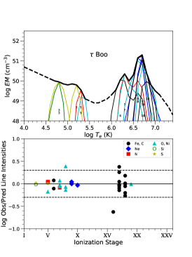
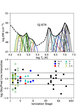
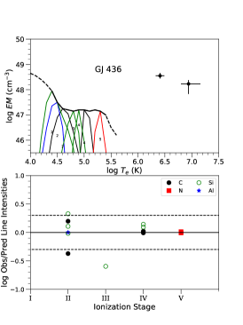
| Ion | (Å) | Ratio | Blends | |||
|---|---|---|---|---|---|---|
| Si xiv | 6.1804 | 7.3 | 5.30e14 | 10.8 | 0.14 | Si xiv 6.1858 |
| Si xiii | 6.6479 | 7.1 | 6.43e14 | 16.1 | 0.59 | Si xiii 6.6882, 6.7403 |
| Mg xii | 7.1058 | 7.1 | 2.85e14 | 12.4 | 0.20 | Mg xii 7.1069, Al xiii 7.1710, 7.1764 |
| Fe xxii | 8.0904 | 7.2 | 5.64e15 | 6.7 | 0.59 | Mg x 8.0696, 8.0701 |
| Fe xxiv | 8.2326 | 7.4 | 2.08e15 | 4.1 | 0.10 | Fe xxii 8.1684, 8.1684, Ni xxi 8.2329, Ni xxiii 8.2685, Fe xxiv 8.2850 |
| Mg xii | 8.4192 | 7.1 | 4.75e14 | 20.0 | 0.09 | Mg xii 8.4246 |
| Mg xi | 9.1687 | 6.9 | 6.22e14 | 25.0 | 0.05 | |
| Mg xi | 9.2312 | 6.9 | 1.43e14 | 12.1 | 0.10 | Mg xi 9.2282, Ne x 9.2461, 9.2912, 9.2913, Ni xix 9.2540, |
| Mg xi | 9.3143 | 6.9 | 3.51e14 | 19.2 | 0.03 | Ne x 9.3616 |
| Ne x | 9.4807 | 6.9 | 2.42e14 | 16.3 | 0.44 | Ne x 9.4809 |
| Ne x | 9.7080 | 6.9 | 2.55e14 | 17.3 | 0.05 | Ne x 9.7085 |
| Na xi | 10.0232 | 7.0 | 3.04e14 | 19.4 | 0.01 | Na xi 10.0286 |
| Fe xvii | 10.1210 | 6.9 | 9.71e15 | 11.1 | 0.26 | Ni xix 10.1100, Fe xix 10.1195, 10.1419 |
| Ne x | 10.2385 | 6.9 | 5.21e14 | 26.0 | 0.04 | Ne x 10.2396 |
| Fe xvii | 10.5040 | 6.9 | 1.75e14 | 15.6 | 0.56 | |
| Fe xviii | 10.5364 | 7.0 | 3.43e15 | 6.9 | 0.00 | |
| Fe xix | 10.6193 | 7.1 | 3.71e14 | 22.9 | 0.15 | Fe xix 10.6001, 10.6116, 10.6840, Fe xxiv 10.6190, 10.6630, Ne ix 10.6426, Fe xvii 10.6570 |
| Fe xvii | 10.7700 | 6.9 | 1.93e14 | 16.7 | 0.18 | Ne ix 10.7650 |
| Fe xix | 10.8160 | 7.1 | 7.97e15 | 10.8 | 0.14 | Fe xix 10.8083 |
| Fe xxiii | 10.9810 | 7.3 | 1.60e14 | 15.4 | 0.02 | |
| Ne ix | 11.0010 | 6.7 | 2.96e14 | 21.1 | 0.15 | Fe xxiii 10.9810, 10.9810, 11.0190, Fe xvii 11.0260, Fe xxiv 11.0290 |
| Fe xvii | 11.1310 | 6.9 | 1.21e14 | 13.6 | 0.01 | |
| Fe xxiv | 11.1760 | 7.4 | 9.15e15 | 11.9 | 0.09 | Fe xxiv 11.1870 |
| Fe xvii | 11.2540 | 6.9 | 2.27e14 | 18.8 | 0.07 | Fe xxiv 11.2680 |
| Fe xviii | 11.4230 | 7.0 | 1.54e14 | 15.7 | 0.16 | Fe xxii 11.4270, Fe xviii 11.4274, Fe xxiv 11.4320, Fe xxiii 11.4580 |
| Ne ix | 11.5440 | 6.7 | 3.76e14 | 24.7 | 0.12 | Fe xviii 11.5270, 11.5270 |
| Fe xxiii | 11.7360 | 7.3 | 2.74e14 | 21.2 | 0.11 | |
| Fe xxii | 11.7700 | 7.2 | 2.16e14 | 18.9 | 0.42 | Fe xxiii 11.7360, 11.7360 |
| Ni xx | 11.8320 | 7.1 | 1.57e14 | 16.2 | 0.16 | Fe xxii 11.8020, Ni xx 11.8460 |
| Fe xxii | 11.9770 | 7.2 | 1.24e14 | 14.6 | 0.14 | Fe xxii 11.8810, 11.9320, 11.9474, Fe xxi 11.9023, 11.9750, Ni xx 11.9617 |
| Fe xviii | 12.0827 | 7.0 | 8.54e15 | 12.2 | 0.53 | Ni xx 12.0787, 12.0879, Fe xxii 12.0928, Ne ix 12.0960 |
| Ne x | 12.1321 | 6.9 | 2.67e13 | 68.6 | 0.19 | Fe xvii 12.1240, Ne x 12.1375 |
| Fe xxii | 12.2100 | 7.2 | 9.26e15 | 12.8 | 0.27 | Fe xxi 12.2040, Ni xxi 12.2080, Fe xix 12.2120 |
| Fe xxi | 12.2840 | 7.2 | 6.88e14 | 35.1 | 0.01 | Fe xvii 12.2660 |
| Ni xix | 12.4350 | 7.0 | 3.16e14 | 24.0 | 0.09 | Fe xxi 12.3930, Fe xx 12.4234, 12.4310 |
| Fe xvi | 12.5399 | 6.8 | 3.00e14 | 23.5 | 0.20 | Fe xxi 12.4990, 12.5048, Fe xx 12.5260, 12.5760, 12.5760, Fe xvii 12.5391 |
| Ni xix | 12.6560 | 7.0 | 1.23e14 | 15.1 | 0.07 | Fe xx 12.6210, Fe xxi 12.6490, Fe xvii 12.6950 |
| Fe xxii | 12.7540 | 7.2 | 1.74e14 | 18.0 | 0.14 | Fe xxi 12.7200, 12.7209,12.7675 |
| Fe xx | 12.8460 | 7.1 | 5.96e14 | 33.3 | 0.06 | Fe xxi 12.8220, Fe xx 12.8240, 12.8640 |
| Fe xx | 12.9120 | 7.1 | 3.91e14 | 26.6 | 0.04 | Fe xix 12.9033, 12.9330, 13.0220, 13.0220, Fe xviii 12.9494, Fe xxii 12.9530, Fe xx 12.9650 |
| Fe xix | 13.0220 | 7.1 | 3.81e15 | 7.1 | 0.22 | |
| Fe xvii | 13.1530 | 6.9 | 1.82e14 | 18.0 | 0.25 | Fe xx 13.1530, 13.1530, 13.1370, 13.1370 |
| Fe xx | 13.2740 | 7.1 | 2.16e14 | 20.4 | 0.21 | Fe xx 13.2453, Fe xix 13.2261, 13.2933, Fe xxii 13.2360, Ni xx 13.2560 |
| Fe xviii | 13.3230 | 7.0 | 1.28e14 | 15.9 | 0.24 | Ni xx 13.3090, Fe xviii 13.3312 |
| Ne ix | 13.4473 | 6.7 | 3.10e13 | 79.2 | 0.03 | Fe xix 13.4970, 13.5180, Ne ix 13.5531 |
| Ne ix | 13.6990 | 6.7 | 1.23e13 | 50.4 | 0.07 | Fe xix 13.6450, 13.7054 |
| Fe xvii | 13.8250 | 6.9 | 9.15e14 | 43.7 | 0.13 | Ni xix 13.7790, Fe xix 13.7950, Fe xvii 13.8920 |
| Fe xviii | 13.9530 | 7.0 | 2.23e14 | 21.6 | 0.43 | Fe xx 13.9620 |
| Ni xix | 14.0430 | 7.0 | 2.60e14 | 23.4 | 0.01 | Fe xxi 14.0080, Fe xix 14.0179, 14.0340, 14.0388 |
| Ni xix | 14.0770 | 7.0 | 1.45e14 | 17.5 | 0.02 | Fe xviii 14.0549, Fe xx 14.0620, 14.0784 |
| Fe xviii | 14.2080 | 7.0 | 1.26e13 | 51.5 | 0.05 | Fe xviii 14.2560 |
| Fe xviii | 14.3730 | 7.0 | 6.33e14 | 36.3 | 0.05 | Fe xviii 14.3430, 14.3990,14.4250, 14.4555 |
| Fe xviii | 14.5340 | 7.0 | 3.95e14 | 28.9 | 0.05 | O viii 14.5242, Fe xviii 14.5608, 14.5710 |
| Fe xix | 14.6640 | 7.1 | 2.44e14 | 22.7 | 0.08 | Fe xviii 14.6160, 14.6566, 14.6887, O viii 14.6343, 14.6344 |
| Fe xx | 14.7540 | 7.1 | 7.96e15 | 13.0 | 0.24 | Fe xix 14.7250, Fe xviii 14.7499, 14.7510, Fe xx 14.7824 |
| Fe xvi | 14.9555 | 6.7 | 3.00e14 | 25.7 | 0.28 | O viii 14.8205, 14.8207, Fe xviii 14.8920, Fe xix 14.9610, 14.9632 |
| Fe xvii | 15.0140 | 6.9 | 2.19e13 | 69.4 | 0.12 | |
| Fe xix | 15.0790 | 7.1 | 3.58e14 | 28.1 | 0.43 | |
| O viii | 15.1760 | 6.6 | 5.28e14 | 34.0 | 0.05 | O viii 15.1765, Fe xix 15.1770, 15.1980 |
| Fe xvii | 15.2610 | 6.9 | 9.18e14 | 44.7 | 0.02 | |
| Fe xviii | 15.3539 | 7.0 | 1.94e14 | 20.2 | 0.08 | Fe xix 15.3123, 15.3340, Fe xvi 15.3694, 15.3907, 15.3926, 15.3992 |
| Fe xvii | 15.4530 | 6.8 | 2.66e14 | 23.9 | 0.03 | Fe xvi 15.4485, 15.4533, 15.5023, Fe xviii 15.4940, Fe xx 15.5170 |
| Fe xviii | 15.6250 | 7.0 | 2.67e14 | 24.3 | 0.10 | |
| Fe xviii | 15.7590 | 7.0 | 4.07e15 | 9.5 | 0.04 | |
| Fe xviii | 15.8240 | 7.0 | 2.24e14 | 21.9 | 0.19 | Fe xviii 15.8700 |
| O viii | 16.0055 | 6.6 | 1.16e13 | 50.5 | 0.11 | Fe xviii 16.0040, O viii 16.0067 |
| Fe xviii | 16.0710 | 7.0 | 5.07e14 | 33.3 | 0.08 | Fe xviii 16.0450 |
| Fe xviii | 16.1590 | 7.0 | 2.25e14 | 22.1 | 0.08 | Fe xix 16.1100 |
| Fe xix | 16.2830 | 7.1 | 1.41e14 | 17.5 | 0.21 | Fe xvii 16.2285, 16.3500, Fe xix 16.2857, Fe xviii 16.3200 |
| Fe xvii | 16.7800 | 6.8 | 1.13e13 | 50.0 | 0.20 | |
| Fe xvii | 17.0510 | 6.8 | 2.85e13 | 79.7 | 0.13 | Fe xvii 17.0960 |
| O vii | 17.3960 | 6.5 | 1.17e14 | 16.1 | 0.35 | Fe xix 17.3908 |
| Fe xviii | 17.6230 | 7.0 | 1.76e14 | 20.0 | 0.23 | |
| O vii | 17.7680 | 6.5 | 1.09e14 | 15.3 | 0.04 | Ar xvi 17.7371, 17.7468 |
| O vii | 18.6270 | 6.4 | 1.81e14 | 20.1 | 0.40 | Ca xviii 18.6909 |
| O viii | 18.9671 | 6.6 | 5.85e13 | 114.0 | 0.04 | O viii 18.9725 |
| N vii | 20.9095 | 6.4 | 1.76e14 | 18.7 | 0.16 | N vii 20.9106 |
| O vii | 21.6015 | 6.4 | 2.19e13 | 66.0 | 0.05 | |
| O vii | 21.8036 | 6.4 | 4.96e14 | 31.1 | 0.17 | |
| O vii | 22.0977 | 6.4 | 1.08e13 | 45.8 | 0.08 | Ca xvi 22.1372 |
| S xiv | 23.0050 | 6.7 | 8.03e15 | 10.5 | 0.16 | |
| N vi | 23.2770 | 6.3 | 5.08e15 | 10.1 | 0.13 | Ca xii 23.2473, Ca xvi 23.2608, Ca xiv 23.2711, Ca xii 23.3326, 23.3326 |
| Ar xvi | 23.5063 | 6.8 | 8.04e15 | 13.3 | 0.53 | Ar xvi 23.5465, Ca xvi 23.5775, Ca xiv 23.5950, 23.6006 |
| N vi | 23.7710 | 6.3 | 5.14e15 | 10.5 | 0.38 |
| Ion | (Å) | Ratio | Blends | |||
|---|---|---|---|---|---|---|
| S xiv | 24.2000 | 6.7 | 4.38e15 | 9.8 | 0.16 | |
| S xiv | 24.2850 | 6.7 | 6.88e15 | 12.2 | 0.08 | |
| S xiv | 24.4180 | 6.7 | 5.82e15 | 11.3 | 0.08 | Ca xiv 24.4046, Ca xv 24.4120, 24.4282, 24.4442, S xiii 24.4175 |
| S xiv | 24.5080 | 6.7 | 1.98e15 | 6.6 | 0.04 | |
| S xiii | 24.5900 | 6.6 | 5.43e15 | 10.9 | 0.47 | |
| N vii | 24.7792 | 6.4 | 9.58e14 | 45.5 | 0.29 | N vii 24.7846 |
| Ar xvi | 24.9942 | 6.8 | 8.89e15 | 13.6 | 0.21 | Ar xvi 25.0098, Ca xiv 25.0636 |
| No id. | 25.1640 | 0.0 | 1.93e15 | 6.4 | … | |
| Ca xi | 25.3270 | 6.4 | 5.08e15 | 10.3 | 0.00 | Ca xiii 25.3503 |
| Ar xvi | 25.5168 | 6.8 | 6.29e15 | 11.3 | 0.13 | Ca xi 25.5170, Ca xiii 25.5301 |
| Ar xvi | 25.6844 | 6.8 | 7.50e15 | 12.1 | 0.11 | |
| C vi | 26.3572 | 6.3 | 7.86e15 | 12.4 | 0.20 | Ca xv 26.2720, Ar xiv 26.2730, C vi 26.3574, Ca xiv 26.3720, Ca xiii 26.3762 |
| Si xii | 26.4560 | 6.5 | 4.05e15 | 8.8 | 0.37 | Ar xiv 26.4300, Si xii 26.4590 |
| C vi | 26.9896 | 6.3 | 2.01e14 | 19.6 | 0.07 | S xiii 26.9792, C vi 26.9901, Ar xv 27.0432 |
| Ar xiv | 27.4640 | 6.7 | 1.50e14 | 16.6 | 0.07 | S xiii 27.3918, Ca xii 27.4131, Ar xiv 27.6360 |
| C vi | 28.4652 | 6.3 | 3.40e14 | 23.6 | 0.12 | Ar xv 28.3464, C vi 28.4663, Ca xii 28.4781 |
| N vi | 28.7870 | 6.3 | 2.48e14 | 19.7 | 0.19 | |
| N vi | 29.0843 | 6.2 | 1.30e14 | 14.0 | 0.14 | Ca xiv 28.9586, 29.1320, Ar xiii 29.1420 |
| S xii | 29.2942 | 6.5 | 8.25e15 | 11.1 | 0.25 | Ar xiv 29.2060, Ca xiv 29.2123, 29.2577, Ar xiii 29.2245 |
| Si xii | 29.4390 | 6.5 | 1.99e14 | 17.0 | 0.22 | Si xii 29.5090, N vi 29.5347 |
| S xiv | 30.4270 | 6.6 | 2.75e14 | 19.2 | 0.46 | Ca xi 30.4480, S xiv 30.4690 |
| Si xii | 31.0120 | 6.5 | 5.82e15 | 8.7 | 0.28 | Si xii 31.0230, S xi 31.0501 |
| Ar xii | 31.3030 | 6.5 | 3.38e15 | 6.6 | 0.39 | |
| S xiii | 32.2391 | 6.6 | 1.05e14 | 11.6 | 0.21 | S xiii 32.1911, Ca xii 32.2805 |
| S xiv | 32.4160 | 6.6 | 1.56e14 | 14.1 | 0.12 | |
| S xiv | 32.5600 | 6.6 | 2.00e14 | 15.7 | 0.39 | S xiv 32.5750, Ca xii 32.6571 |
| S xiv | 33.5490 | 6.6 | 1.40e14 | 12.9 | 0.11 | |
| C vi | 33.7342 | 6.2 | 1.69e13 | 45.0 | 0.23 | C vi 33.7396 |
| S xiii | 33.9461 | 6.5 | 1.23e14 | 11.9 | 0.63 | S xiii 33.9526, Fe xvii 33.9618 |
| C v | 34.9728 | 6.1 | 7.26e15 | 9.0 | 0.26 | Ar ix 35.0240, Fe xvi 35.1059 |
| Fe xvii | 35.6844 | 6.9 | 1.86e14 | 14.5 | 0.13 | Ca xi 35.7370 |
| Fe xviii | 93.9230 | 7.0 | 1.10e14 | 3.8 | 0.80 | Fe xx 93.7800 |
| Ne viii | 98.2600 | 5.9 | 2.31e14 | 5.7 | 0.04 | Fe xxi 97.8800, Ne viii 98.1150, 98.2740 |
| Fe xx | 121.8300 | 7.1 | 1.63e14 | 4.5 | 0.14 | |
| Fe xxi | 128.7300 | 7.2 | 1.40e14 | 3.5 | 0.37 | |
| Fe xxiii | 132.8500 | 7.3 | 4.22e14 | 6.5 | 0.34 | Fe xx 132.8500 |
| Fe xxii | 135.7800 | 7.2 | 1.45e14 | 3.2 | 0.28 | Fe xi 135.6988 |
| Fe xv | 284.1630 | 6.4 | 1.53e13 | 4.3 | 0.04 | |
| Fe xvi | 335.4099 | 6.5 | 1.80e13 | 6.6 | 0.07 | Fe xiv 334.1800 |
| Mg ix | 368.0577 | 6.1 | 9.96e14 | 4.5 | 0.01 | |
| S xiv | 417.6655 | 6.6 | 1.17e13 | 3.2 | 0.06 | Fe xv 417.2580 |
| S vi | 933.3788 | 5.4 | 2.28e15 | 3.6 | 0.22 | |
| O vi | 1031.9121 | 5.6 | 1.42e13 | 18.2 | 0.31 | |
| C ii | 1036.3390 | 4.8 | 2.34e15 | 6.6 | 0.61 | |
| C ii | 1037.0200 | 4.8 | 8.05e15 | 8.7 | 0.37 | |
| O vi | 1037.6136 | 5.6 | 7.04e14 | 15.5 | 0.31 | |
| Si iii | 1108.3610 | 4.9 | 1.22e15 | 4.6 | 0.01 | |
| Si iii | 1109.9720 | 4.9 | 1.74e15 | 5.3 | 0.20 | Si iii 1109.9430 |
| Si iv | 1122.4852 | 5.0 | 7.56e16 | 5.0 | 0.14 | |
| Si iv | 1128.3404 | 5.0 | 1.64e15 | 6.4 | 0.23 | |
| Ne v | 1145.5959 | 5.5 | 5.90e16 | 5.7 | 0.28 | |
| C iii | 1176.0000 | 4.8 | 5.81e14 | 7.5 | 0.31 | |
| C iii | 1176.0000 | 4.8 | 6.20e14 | 20.9 | 0.28 | |
| S iii | 1200.9610 | 4.9 | 3.18e15 | 42.6 | 0.10 | |
| O v | 1218.3440 | 5.5 | 1.40e14 | 104.6 | 0.17 | |
| N v | 1238.8218 | 5.4 | 4.28e14 | 74.6 | 0.20 | |
| N v | 1242.8042 | 5.4 | 2.02e14 | 45.8 | 0.17 | |
| C iii | 1247.3830 | 5.1 | 6.29e16 | 18.7 | 0.21 | |
| Si ii | 1264.7400 | 4.5 | 1.64e15 | 20.6 | 0.03 | |
| Si ii | 1265.0040 | 4.6 | 1.06e15 | 48.7 | 0.08 | |
| Si iii | 1294.5480 | 4.9 | 8.71e16 | 12.5 | 0.70 | |
| Si iii | 1296.7280 | 4.9 | 9.89e16 | 31.3 | 0.35 | |
| Si iii | 1298.9480 | 4.9 | 2.30e15 | 35.0 | 0.65 | |
| Si iii | 1301.1510 | 4.9 | 6.32e16 | 15.3 | 0.63 | |
| Si iii | 1303.3249 | 4.9 | 8.65e16 | 33.3 | 0.20 | |
| Si ii | 1304.3719 | 4.6 | 4.01e16 | 26.3 | 0.20 | |
| Si ii | 1309.2770 | 4.6 | 7.10e16 | 15.1 | 0.25 | |
| C ii | 1323.9080 | 4.8 | 4.07e16 | 11.9 | 0.55 | C ii 1323.9540 |
| Fe xix | 1328.6999 | 7.1 | 4.21e16 | 23.4 | 0.44 | |
| C ii | 1334.5350 | 4.7 | 1.75e14 | 43.7 | 0.66 | |
| C ii | 1335.7100 | 4.7 | 4.45e14 | 69.5 | 0.05 | C ii 1335.6650 |
| Fe xii | 1349.4000 | 6.3 | 4.75e16 | 38.4 | 0.01 | |
| O v | 1371.2960 | 5.5 | 2.22e15 | 22.4 | 0.03 | |
| Si iv | 1393.7552 | 5.0 | 2.34e14 | 70.3 | 0.11 | |
| O iv | 1397.2309 | 5.3 | 7.47e16 | 24.2 | 0.49 | |
| Si iv | 1402.7704 | 5.0 | 1.14e14 | 82.1 | 0.12 | |
| S iv | 1406.0160 | 5.1 | 4.28e15 | 77.5 | 0.06 | |
| Fe xi | 1467.4230 | 6.2 | 3.28e16 | 12.1 | 0.07 | |
| Si ii | 1526.7090 | 4.5 | 1.58e15 | 25.5 | 0.04 | |
| Si ii | 1533.4320 | 4.5 | 2.60e15 | 25.7 | 0.04 |
| Ion | (Å) | Ratio | Blends | |||
|---|---|---|---|---|---|---|
| C iv | 1548.1871 | 5.1 | 1.31e13 | 71.8 | 0.16 | |
| C iv | 1550.7723 | 5.1 | 6.60e14 | 40.6 | 0.16 | |
| Al ii | 1670.7870 | 4.6 | 1.12e14 | 20.8 | 0.01 |
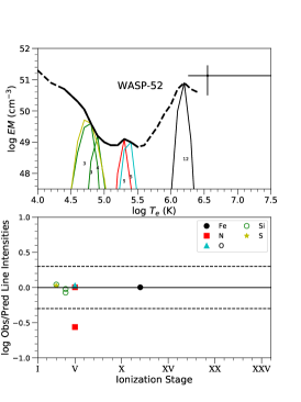
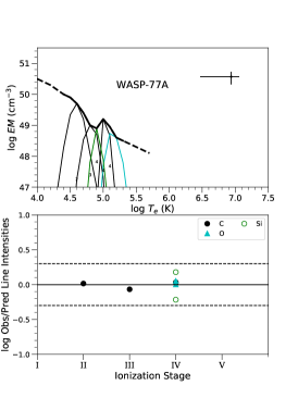
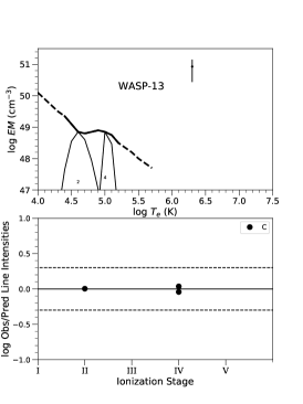
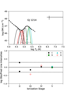
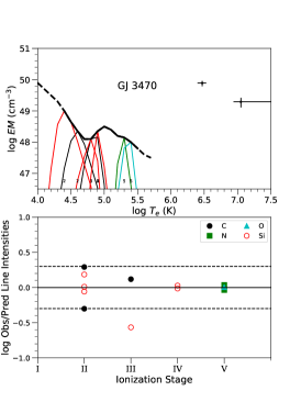
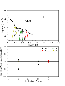
| Ion | (Å) | Ratio | Blends | |||
|---|---|---|---|---|---|---|
| Mg xii | 8.4192 | 7.1 | 2.58e14 | 9.5 | 0.43 | Mg xii 8.4246 |
| Mg xi | 9.1687 | 6.9 | 5.81e14 | 15.9 | 0.02 | Fe xxi 9.1944 |
| Mg xi | 9.2312 | 6.9 | 2.47e14 | 10.5 | 0.15 | Fe xxii 9.2298, Ne x 9.2461, 9.2462, Ne x 9.2912, 9.2913 |
| Mg xi | 9.3143 | 6.9 | 5.40e14 | 15.7 | 0.14 | Ne x 9.3616 |
| Ne x | 9.4807 | 6.9 | 4.07e14 | 13.9 | 0.02 | Ne x 9.4809 |
| Ne x | 9.7080 | 6.9 | 6.78e14 | 18.5 | 0.14 | Ne x 9.7085 |
| Ne x | 10.2385 | 6.9 | 1.43e13 | 28.2 | 0.23 | Ne x 10.2396 |
| Fe xviii | 10.5364 | 7.0 | 3.38e14 | 14.2 | 0.04 | Fe xvii 10.5040, Fe xviii 10.5382, 10.5640, Ne ix 10.5406, 10.5650 |
| Fe xix | 10.6193 | 7.1 | 5.43e14 | 18.2 | 0.09 | Fe xix 10.6001, 10.6116, 10.6840, Fe xxiv 10.6190, 10.6630, Ne ix 10.6426, Fe xvii 10.6570 |
| Fe xvii | 10.7700 | 6.9 | 2.40e14 | 12.3 | 0.10 | Fe xix 10.7650, Ne ix 10.7650 |
| Fe xxiii | 10.9810 | 7.3 | 8.26e14 | 22.8 | 0.01 | Ne ix 11.0010, Fe xxiii 11.0190, Fe xvii 11.0260, Fe xxiv 11.0290 |
| Fe xxiv | 11.1760 | 7.4 | 3.13e14 | 14.5 | 0.11 | Fe xvii 11.1310 |
| Fe xvii | 11.2540 | 6.9 | 3.99e14 | 16.4 | 0.08 | Fe xxiv 11.2680 |
| Fe xviii | 11.4230 | 7.0 | 3.20e14 | 14.6 | 0.20 | Fe xxii 11.4270, Fe xviii 11.4274, Fe xxiv 11.4320, Fe xxiii 11.4580 |
| Ne ix | 11.5440 | 6.7 | 1.22e13 | 27.7 | 0.04 | Fe xviii 11.5270 |
| Fe xxii | 11.7700 | 7.2 | 9.03e14 | 25.5 | 0.07 | Fe xxiii 11.7360 |
| Ni xx | 11.8320 | 7.1 | 4.61e15 | 5.8 | 0.24 | Ni xx 11.8460 |
| Fe xxii | 11.9770 | 7.2 | 3.37e14 | 16.0 | 0.09 | Fe xxii 11.8810, 11.9320, 11.9474, Fe xxi 11.9023, 11.9750 |
| Ne x | 12.1321 | 6.9 | 9.03e13 | 83.7 | 0.25 | Ne x 12.1375 |
| Fe xxi | 12.2840 | 7.2 | 1.31e13 | 32.2 | 0.08 | Fe xvii 12.2660 |
| Ni xix | 12.4350 | 7.0 | 9.12e14 | 27.1 | 0.04 | Fe xxi 12.3930, 12.4990, Fe xx 12.4234, 12.4310, 12.5760 |
| Fe xxi | 12.6490 | 7.2 | 4.33e14 | 18.9 | 0.48 | Ni xix 12.6560, Fe xvii 12.6950 |
| Fe xx | 12.8460 | 7.1 | 1.09e13 | 29.9 | 0.14 | Fe xxi 12.8220, Fe xx 12.8240, 12.8640 |
| Fe xx | 12.9120 | 7.1 | 8.79e14 | 26.4 | 0.07 | Fe xix 12.9033, 12.9330, 13.0220, Fe xviii 12.9494, Fe xxii 12.9530, Fe xx 12.9650, 12.9920 |
| Fe xx | 13.1530 | 7.1 | 3.72e14 | 15.1 | 0.16 | Fe xx 13.1530, 13.1370,13.1370 |
| Fe xx | 13.2740 | 7.1 | 5.00e14 | 20.6 | 0.03 | Fe xix 13.2261, 13.2933, Fe xxii 13.2360, Fe xx 13.2453, Ni xx 13.3090, Fe xviii 13.3230 |
| Ne ix | 13.4473 | 6.7 | 8.00e13 | 83.6 | 0.04 | Fe xix 13.4970, 13.5180, Ne ix 13.5531 |
| Ne ix | 13.6990 | 6.7 | 4.01e13 | 59.5 | 0.10 | Fe xix 13.7054 |
| Fe xvii | 13.8250 | 6.9 | 1.79e13 | 40.2 | 0.13 | Fe xix 13.7590, 13.7950, 13.8390, Fe xx 13.7670, Ni xix 13.7790, Fe xvii 13.8920 |
| Fe xx | 13.9620 | 7.1 | 4.74e14 | 20.8 | 0.40 | Fe xviii 13.9530 |
| Fe xxi | 14.0080 | 7.2 | 3.97e14 | 19.0 | 0.09 | Fe xix 14.0179, Cr xxi 14.0339, Fe xix 14.0340, 14.0388, Ni xix 14.0430 |
| Ni xix | 14.0770 | 7.0 | 4.23e14 | 19.7 | 0.42 | Fe xviii 14.0549, Fe xx 14.0620, 14.0784 |
| Fe xviii | 14.2080 | 7.0 | 2.68e13 | 49.5 | 0.07 | Fe xviii 14.2560 |
| Fe xviii | 14.3730 | 7.0 | 1.40e13 | 35.7 | 0.06 | Fe xviii 14.3430, 14.3990, 14.4250, 14.4555 |
| Fe xviii | 14.5340 | 7.0 | 1.06e13 | 31.5 | 0.01 | O viii 14.5242, 14.5243, Fe xviii 14.5608, 14.5710 |
| Fe xix | 14.6640 | 7.1 | 7.88e14 | 27.2 | 0.17 | O viii 14.6343, 14.6344, Fe xix 14.7250, Fe xviii 14.7499, Fe xx 14.7540 |
| O viii | 14.8205 | 6.6 | 5.21e14 | 22.3 | 0.03 | O viii 14.8207 |
| Fe xix | 14.9610 | 7.1 | 2.41e14 | 15.2 | 0.38 | Fe xx 14.8791, 14.9279, Fe xviii 14.8920, 14.9717, Fe xix 14.8995, 14.9170, 14.9632 |
| Fe xvii | 15.0140 | 6.9 | 3.79e13 | 60.4 | 0.09 | |
| Fe xix | 15.0790 | 7.1 | 5.52e14 | 23.1 | 0.19 | |
| O viii | 15.1760 | 6.6 | 1.47e13 | 37.3 | 0.08 | O viii 15.1765, Fe xix 15.1770, 15.1980 |
| Fe xvii | 15.2610 | 6.9 | 1.54e13 | 38.1 | 0.04 | |
| Fe xviii | 15.3539 | 7.0 | 3.59e14 | 18.0 | 0.03 | Fe xix 15.3123, 15.3340, 15.3709, Fe xvi 15.3907 |
| Fe xvii | 15.4530 | 6.8 | 4.93e14 | 21.2 | 0.07 | Fe xvi 15.4533, Fe xviii 15.4940, Fe xx 15.5170 |
| Fe xviii | 15.6250 | 7.0 | 4.65e14 | 21.1 | 0.19 | |
| Fe xviii | 15.7590 | 7.0 | 1.19e14 | 10.8 | 0.10 | |
| Fe xviii | 15.8700 | 7.0 | 4.65e14 | 21.1 | 0.20 | Fe xviii 15.8240 |
| O viii | 16.0055 | 6.6 | 2.99e13 | 54.4 | 0.16 | Fe xviii 16.0040, O viii 16.0067 |
| Fe xviii | 16.0710 | 7.0 | 1.11e13 | 33.1 | 0.06 | Fe xviii 16.0450 |
| Fe xviii | 16.1590 | 7.0 | 1.79e14 | 13.1 | 0.58 | Fe xix 16.1100 |
| Fe xix | 16.2830 | 7.1 | 2.92e14 | 16.8 | 0.23 | Fe xvii 16.2285, 16.3500, Fe xix 16.2857,16.3247, Fe xviii 16.3200 |
| Fe xvii | 16.7800 | 6.8 | 2.12e13 | 45.7 | 0.12 | |
| Fe xvii | 17.0510 | 6.8 | 5.23e13 | 70.5 | 0.06 | Fe xvii 17.0960 |
| O vii | 17.3960 | 6.5 | 3.61e14 | 18.1 | 0.07 | Cr xviii 17.4031, Cr xvi 17.4207, 17.4252 |
| Fe xviii | 17.6230 | 7.0 | 4.55e14 | 21.0 | 0.15 | |
| O vii | 17.7680 | 6.5 | 3.50e14 | 17.8 | 0.08 | Ar xvi 17.7371, 17.7468 |
| O vii | 18.6270 | 6.4 | 6.85e14 | 26.5 | 0.30 | Ca xviii 18.6909 |
| O viii | 18.9671 | 6.6 | 1.41e12 | 119.3 | 0.16 | O viii 18.9725 |
| N vii | 20.9095 | 6.4 | 4.56e14 | 20.4 | 0.26 | |
| Ca xvi | 21.4501 | 6.8 | 1.64e14 | 12.6 | 0.56 | |
| O vii | 21.6015 | 6.4 | 3.59e13 | 59.0 | 0.04 | |
| O vii | 21.8036 | 6.4 | 7.47e14 | 26.8 | 0.07 | |
| No id. | 21.9686 | 0.0 | 1.11e14 | 10.3 | … | |
| O vii | 22.0977 | 6.4 | 2.65e13 | 50.2 | 0.02 | Ca xvi 22.1372 |
| S xiv | 23.0050 | 6.7 | 1.56e14 | 10.2 | 0.05 | S xiv 23.0150, Ca xv 23.0230, Ca xvi 23.0433 |
| N vi | 23.1274 | 6.3 | 1.34e14 | 9.6 | 0.16 | Ca xiv 23.1518, Ca xvii 23.1752, Ca xv 23.1818, Ca xii 23.1892 |
| N vi | 23.2770 | 6.3 | 1.64e14 | 12.5 | 0.39 | Ca xii 23.2473, 23.3326, Ca xvi 23.2608, Ca xiv 23.2711 |
| Ar xvi | 23.5063 | 6.8 | 3.67e14 | 19.3 | 0.05 | Ca xv 23.5034 |
| Ar xvi | 23.5465 | 6.8 | 1.38e14 | 11.9 | 0.14 | Ca xiv 23.6006 |
| No id. | 23.7700 | 0.0 | 3.14e14 | 12.6 | … | |
| Ca xiv | 24.0860 | 6.7 | 2.16e14 | 15.2 | 0.36 | Ca xiv 24.0335 |
| S xiv | 24.2000 | 6.7 | 2.48e14 | 16.4 | 0.38 | Ca xiv 24.1331, Ca xvi 24.2214, Ca xv 24.2344 |
| S xiv | 24.2850 | 6.7 | 2.13e14 | 15.2 | 0.12 | Ca xiv 24.2599, S xiv 24.2890 |
| S xiv | 24.4180 | 6.7 | 2.46e14 | 16.3 | 0.16 | Ca xv 24.3365, 24.4120, 24.4282, 24.4442, Ca xiv 24.4046 |
| S xiii | 24.5900 | 6.6 | 2.61e14 | 16.8 | 0.48 | S xiv 24.5080, Si xiii 24.5172, Ca xv 24.5274 |
| N vii | 24.7792 | 6.4 | 1.97e13 | 45.3 | 0.16 | Ar xv 24.7400, N vii 24.7846, Ar xvi 24.8509 |
| Ar xvi | 24.9942 | 6.8 | 5.24e14 | 23.4 | 0.04 | Ar xvi 25.0098 |
| No id. | 25.2000 | 0.0 | 1.15e14 | 11.0 | … | |
| Ca xi | 25.3270 | 6.4 | 1.55e14 | 12.8 | 0.27 | Ca xiii 25.3503 |
| Ar xvi | 25.5168 | 6.8 | 2.21e14 | 15.2 | 0.28 | Ca xv 25.4749, Ca xi 25.5170, Ca xiii 25.5301 |
| Ar xvi | 25.6844 | 6.8 | 7.53e14 | 27.0 | 0.28 | Si xii 25.6580, Ca xiv 25.7299, Ca xvi 25.7330 |
| C vi | 26.3572 | 6.3 | 3.33e14 | 18.3 | 0.03 | Ca xv 26.2720, Ar xiv 26.2730, C vi 26.3574, Ca xiv 26.3720, Ca xiii 26.3762 |
| Si xii | 26.4560 | 6.5 | 4.21e14 | 20.4 | 0.36 | Ar xiv 26.4300, Si xii 26.4590, Ca xiv 26.5141, Ca xiii 26.5862 |
| C vi | 26.9896 | 6.3 | 7.35e14 | 26.8 | 0.13 | C vi 26.9901, Si xii 27.0350, Ar xv 27.0432 |
| Ion | (Å) | Ratio | Blends | |||
|---|---|---|---|---|---|---|
| Ar xiv | 27.4640 | 6.7 | 4.55e14 | 20.9 | 0.32 | S xiii 27.3918, Ca xii 27.4131 |
| Fe xvii | 27.5097 | 6.9 | 3.14e14 | 16.8 | 0.53 | S xv 27.5300, 27.5598, Ar xiv 27.5490, 27.6310, 27.6360, Ar xv 27.5559 |
| C vi | 28.4652 | 6.3 | 7.51e14 | 25.8 | 0.04 | Ar xv 28.3464, C vi 28.4663, Ca xii 28.4781 |
| Ca xii | 28.6811 | 6.5 | 1.40e14 | 11.1 | 0.34 | Ca xii 28.6131, 28.6370 |
| N vi | 28.7870 | 6.3 | 1.46e14 | 11.3 | 0.27 | |
| Ca xiii | 28.9161 | 6.6 | 1.37e14 | 11.0 | 0.21 | Ar xiv 28.8940 |
| N vi | 29.0843 | 6.2 | 3.69e14 | 17.2 | 0.17 | Ca xiv 29.1320, Ar xiii 29.1420 |
| Ar xiii | 29.2245 | 6.6 | 3.31e14 | 15.9 | 0.47 | Ar xiv 29.2060, Ca xiv 29.2123, 29.2577, Ar xv 29.2210 |
| N vi | 29.5347 | 6.2 | 4.96e14 | 19.8 | 0.10 | Si xii 29.4390, 29.5090 |
| S xiv | 30.4270 | 6.6 | 4.68e14 | 18.6 | 0.40 | Ca xi 30.4480, S xiv 30.4690 |
| Ca xiii | 30.5402 | 6.6 | 1.32e14 | 9.8 | 0.64 | Ca x 30.5033 |
| Ca xi | 30.8670 | 6.4 | 1.59e14 | 10.9 | 0.26 | Ar xiv 30.8320, Ar xiii 30.8854 |
| Si xii | 31.0120 | 6.5 | 3.50e14 | 15.9 | 0.27 | Si xii 31.0230 |
| Fe xvii | 31.9515 | 6.9 | 3.04e14 | 15.0 | 0.45 | Fe xvii 31.8776, Ar xiii 31.8954, Ca xii 31.9561, Ar xiv 32.0140 |
| Fe xvii | 32.1188 | 6.9 | 1.07e14 | 8.9 | 0.51 | Fe xvii 32.0941, Ca xii 32.1057, Fe xvi 32.1658 |
| S xiii | 32.2391 | 6.6 | 3.84e14 | 16.8 | 0.18 | S xiii 32.1911, Ca xii 32.2805 |
| S xiv | 32.4160 | 6.6 | 3.38e14 | 15.7 | 0.04 | Ca xii 32.4184 |
| S xiv | 32.5600 | 6.6 | 6.38e14 | 21.2 | 0.13 | Ca xii 32.4988, 32.6571, S xiv 32.5750 |
| S xiv | 33.3810 | 6.6 | 1.52e14 | 10.2 | 0.10 | |
| C v | 33.4257 | 6.1 | 1.13e14 | 8.9 | 0.29 | Ca xiii 33.4080, Si xiv 33.4444, Ar xiv 33.4600 |
| S xiv | 33.5490 | 6.6 | 3.65e14 | 15.5 | 0.05 | Si xiv 33.5051, Si xi 33.5301, 33.5731 |
| C vi | 33.7342 | 6.2 | 2.89e13 | 44.2 | 0.08 | C vi 33.7396 |
| Fe xvii | 33.8758 | 6.9 | 1.38e14 | 9.5 | 0.33 | Fe xvii 33.8863, Si xi 33.9070, S xiii 33.9461, 33.9526 |
| C v | 34.9728 | 6.1 | 2.57e14 | 12.9 | 0.47 | Ar xiii 34.8385, Fe xvi 34.8569, Ar ix 35.0240 |
| Ca xi | 35.2130 | 6.4 | 3.40e14 | 14.7 | 0.00 | |
| Si xi | 35.4374 | 6.3 | 1.33e14 | 9.4 | 0.40 | S xii 35.3990, Ca xiii 35.4444 |
| Ca xi | 35.5760 | 6.4 | 1.07e14 | 8.5 | 0.33 | |
| Fe xvii | 35.6844 | 6.9 | 3.39e14 | 14.7 | 0.21 | Fe xxi 35.6238, Ca xi 35.7370 |
| Fe xviii | 93.9230 | 7.0 | 1.04e13 | 9.1 | 0.11 | Fe xx 93.7800 |
| Ne viii | 98.2600 | 5.9 | 1.02e13 | 9.8 | 0.26 | Fe xxi 97.8800, Ne viii 98.1150, 98.2740 |
| Fe xix | 101.5500 | 7.0 | 4.85e14 | 7.3 | 0.11 | |
| Fe xxi | 102.2200 | 7.2 | 1.03e13 | 11.0 | 0.20 | O viii 102.3476, 102.3552, 102.3919, 102.4897, 102.5497 |
| Ne viii | 103.0850 | 5.9 | 3.27e14 | 5.6 | 0.30 | Fe ix 103.5662 |
| Fe xviii | 103.9370 | 7.0 | 2.42e14 | 4.8 | 0.22 | |
| Fe xix | 106.3300 | 7.0 | 2.38e14 | 3.9 | 0.38 | Ni xxii 106.0640, Fe xix 106.1200, Ne vii 106.1900 |
| Fe xix | 108.3700 | 7.0 | 9.00e14 | 9.6 | 0.06 | Fe xxi 108.1200 |
| Fe xix | 109.9700 | 7.0 | 2.91e14 | 4.7 | 0.21 | |
| Fe xxii | 114.4100 | 7.2 | 3.06e14 | 4.9 | 0.26 | |
| Fe xxii | 117.1700 | 7.2 | 1.27e13 | 12.5 | 0.10 | Fe xxi 117.5100 |
| Ni xxii | 117.9330 | 7.2 | 2.32e14 | 3.9 | 0.15 | Ni xxv 117.9330, Si v 117.8540, Cr xx 117.9580 |
| Fe xx | 118.6600 | 7.1 | 4.72e14 | 6.7 | 0.14 | |
| Fe xx | 121.8300 | 7.1 | 5.56e14 | 7.3 | 0.06 | |
| Fe xxi | 128.7300 | 7.2 | 1.18e13 | 10.8 | 0.11 | |
| Fe xxiii | 132.8500 | 7.3 | 3.76e13 | 20.7 | 0.19 | Fe xx 132.8500 |
| Fe xxii | 135.7800 | 7.2 | 8.62e14 | 8.7 | 0.09 | |
| Fe ix | 171.0730 | 6.0 | 7.18e14 | 4.7 | 0.04 | O v 172.1690 |
| Fe xi | 182.1690 | 6.2 | 4.85e14 | 3.7 | 0.59 | C vi 182.0969, 182.1323, C vi 182.2304, 182.2900, Fe x 182.3070 |
| Fe xxiv | 192.0170 | 7.4 | 2.86e13 | 11.0 | 0.29 | Ca xvii 192.8532 |
| Fe xiii | 197.4330 | 6.3 | 4.94e14 | 3.4 | 0.70 | Fe xiii 196.7675, 196.8215, Fe ix 197.3784 |
| Ar xv | 221.1356 | 6.7 | 8.41e14 | 4.7 | 0.26 | S xii 221.4005 |
| S xiii | 256.6852 | 6.5 | 1.50e13 | 6.9 | 0.38 | He ii 256.3183, 256.3194, Si x 256.3660 |
| S x | 264.2306 | 6.3 | 5.58e14 | 3.7 | 0.03 | Fe xiv 264.7900 |
| Si x | 277.2780 | 6.2 | 3.89e14 | 3.1 | 0.18 | |
| Fe xv | 284.1630 | 6.4 | 1.96e13 | 8.4 | 0.00 | |
| Si viii | 314.3560 | 6.0 | 5.45e14 | 3.6 | 0.13 | |
| Fe xvi | 335.4099 | 6.5 | 1.55e13 | 9.8 | 0.23 | Fe xiv 334.1800 |
| Ar xvi | 353.8535 | 6.8 | 7.21e14 | 6.4 | 0.26 | |
| Fe xvi | 360.7580 | 6.5 | 9.12e14 | 7.3 | 0.18 | Ne v 359.3750 |
| Mg ix | 368.0577 | 6.1 | 3.78e14 | 4.1 | 0.38 | |
| S xiv | 417.6655 | 6.6 | 6.55e14 | 4.0 | 0.42 | Fe xv 417.2580 |
| Ne vi | 558.6850 | 5.7 | 1.48e13 | 4.1 | 0.25 | O iv 555.2630, Ca x 557.7640, Ne v 568.4220 |
| S vi | 933.3788 | 5.4 | 3.57e15 | 3.3 | 0.21 | |
| N iii | 991.5770 | 5.0 | 7.91e15 | 4.8 | 0.41 | |
| Ne vi | 999.1830 | 5.7 | 4.52e15 | 4.0 | 0.45 | |
| Ne vi | 1010.2050 | 5.7 | 1.90e15 | 4.2 | 0.48 | |
| S iii | 1021.3230 | 4.9 | 2.05e15 | 5.5 | 0.31 | |
| O vi | 1031.9121 | 5.6 | 2.29e13 | 16.0 | 0.15 | |
| C ii | 1036.3390 | 4.8 | 8.63e15 | 6.2 | 0.28 | |
| C ii | 1037.0200 | 4.8 | 1.71e14 | 7.2 | 0.29 | |
| O vi | 1037.6136 | 5.6 | 1.15e13 | 13.7 | 0.15 | |
| S iv | 1062.6639 | 5.1 | 2.04e15 | 7.0 | 0.73 | |
| S iv | 1072.9740 | 5.1 | 5.14e15 | 8.4 | 0.14 | |
| S iii | 1077.1730 | 4.9 | 1.99e15 | 8.7 | 0.16 | |
| N ii | 1085.7030 | 4.7 | 1.16e14 | 3.4 | 0.39 | N ii 1085.5310, 1085.5480 |
| Si iii | 1108.3610 | 4.9 | 2.09e15 | 6.4 | 0.08 | |
| Si iii | 1109.9720 | 4.9 | 5.92e15 | 6.3 | 0.19 | |
| Si iii | 1113.2320 | 4.9 | 5.90e15 | 7.3 | 0.19 | Si iii 1113.2061 |
| Fe xix | 1118.0699 | 7.0 | 5.73e15 | 6.4 | 0.19 | |
| Si iv | 1122.4852 | 5.0 | 5.01e15 | 7.1 | 0.39 | |
| Si iv | 1128.3404 | 5.0 | 4.55e15 | 6.7 | 0.05 | Si iv 1128.3252 |
| Ne v | 1145.5959 | 5.5 | 2.01e15 | 6.3 | 0.37 | |
| S iii | 1190.1990 | 4.9 | 2.80e15 | 8.1 | 0.13 | |
| Si ii | 1190.4170 | 4.6 | 1.53e15 | 4.8 | 0.07 | |
| S iii | 1194.0490 | 4.9 | 4.81e15 | 11.8 | 0.45 |
| Ion | (Å) | Ratio | Blends | |||
|---|---|---|---|---|---|---|
| Si ii | 1194.5010 | 4.6 | 4.36e15 | 13.7 | 0.36 | S iii 1194.4430 |
| S iii | 1200.9610 | 4.9 | 8.55e15 | 23.6 | 0.74 | |
| Si iii | 1206.5019 | 4.9 | 1.24e13 | 35.7 | 0.68 | |
| O v | 1218.3440 | 5.5 | 2.26e14 | 77.0 | 0.22 | |
| N v | 1238.8218 | 5.4 | 6.78e14 | 37.0 | 0.12 | |
| N v | 1242.8042 | 5.4 | 3.30e14 | 23.2 | 0.11 | |
| C iii | 1247.3830 | 5.1 | 6.14e15 | 11.5 | 0.40 | |
| S ii | 1259.5210 | 4.6 | 3.03e15 | 12.6 | 0.04 | |
| Si ii | 1264.7400 | 4.5 | 6.67e15 | 13.4 | 0.13 | |
| Si ii | 1265.0040 | 4.6 | 3.80e15 | 15.9 | 0.20 | |
| Si iii | 1296.7280 | 4.9 | 4.88e15 | 17.2 | 0.72 | |
| Si iii | 1303.3249 | 4.9 | 4.96e15 | 19.7 | 0.64 | |
| Si ii | 1304.3719 | 4.6 | 1.91e15 | 9.3 | 0.22 | |
| Si ii | 1309.2770 | 4.6 | 4.61e15 | 15.7 | 0.14 | |
| Si iii | 1312.5930 | 4.9 | 1.80e15 | 9.5 | 0.42 | |
| C ii | 1323.9080 | 4.8 | 2.88e15 | 8.7 | 0.39 | |
| Fe xix | 1328.6999 | 7.1 | 9.39e16 | 6.3 | 0.51 | |
| C ii | 1334.5350 | 4.7 | 9.08e14 | 56.4 | 0.25 | |
| C ii | 1335.7100 | 4.7 | 1.96e13 | 59.7 | 0.44 | |
| O iv | 1338.6140 | 5.3 | 1.16e15 | 9.0 | 0.49 | |
| Fe xxi | 1354.0800 | 7.2 | 7.92e15 | 13.6 | 0.27 | |
| O v | 1371.2960 | 5.5 | 4.95e15 | 18.6 | 0.27 | |
| Si iv | 1393.7552 | 5.0 | 1.26e13 | 33.2 | 0.13 | |
| Si iv | 1402.7704 | 5.0 | 7.09e14 | 25.3 | 0.18 | |
| S iv | 1406.0160 | 5.1 | 9.56e16 | 16.3 | 0.59 | |
| Cr xvi | 1410.5990 | 6.8 | 4.83e16 | 14.2 | 0.06 | |
| S v | 1501.7660 | 5.3 | 1.26e15 | 21.3 | 0.04 | |
| Si ii | 1526.7090 | 4.5 | 8.62e15 | 19.6 | 0.03 | |
| Si ii | 1533.4320 | 4.5 | 1.03e14 | 9.7 | 0.19 | |
| C iv | 1548.1871 | 5.1 | 4.30e13 | 49.9 | 0.04 | |
| C iv | 1550.7723 | 5.1 | 2.24e13 | 35.3 | 0.06 | |
| Al ii | 1670.7870 | 4.6 | 2.35e14 | 27.1 | 0.02 |
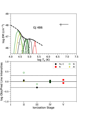
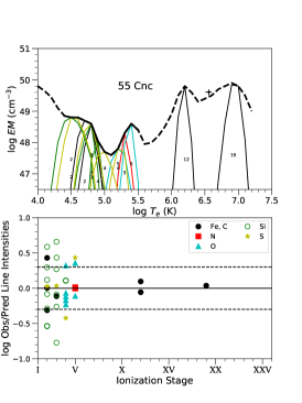
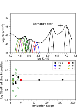
| Ion | (Å) | Ratio | Blends | |||
|---|---|---|---|---|---|---|
| Fe xvii | 11.2540 | 6.9 | 2.68e14 | 7.2 | 0.38 | Fe xviii 11.3260, 11.3260, 11.3260 |
| Ne x | 12.1321 | 6.9 | 4.70e14 | 4.1 | 0.03 | Fe xvii 12.1240, Ne x 12.1375 |
| Fe xvii | 12.2660 | 6.9 | 1.50e14 | 3.0 | 0.10 | |
| Ne ix | 13.4473 | 6.7 | 5.02e14 | 7.7 | 0.04 | Fe xix 13.5180, Ne ix 13.5531 |
| Ne ix | 13.6990 | 6.7 | 2.10e14 | 7.3 | 0.00 | |
| Fe xvii | 13.8250 | 6.9 | 1.97e14 | 5.0 | 0.14 | Ni xix 13.7790, Fe xvii 13.8920 |
| Ni xix | 14.0430 | 7.0 | 2.53e14 | 6.9 | 0.01 | Fe xviii 13.9530, Ni xix 14.0770 |
| Fe xviii | 14.2080 | 7.0 | 2.70e14 | 7.9 | 0.06 | Fe xviii 14.2560 |
| Fe xviii | 14.3730 | 7.0 | 1.15e14 | 4.6 | 0.20 | Fe xviii 14.3430, 14.3430, 14.3990, 14.4250, 14.4250, 14.4555 |
| Fe xviii | 14.5340 | 7.0 | 5.76e15 | 3.7 | 0.26 | O viii 14.5242, Fe xviii 14.5608, 14.5710, 14.6160 |
| Fe xvi | 14.9555 | 6.7 | 2.28e15 | 3.5 | 0.63 | Fe xix 14.9610 |
| Fe xvii | 15.0140 | 6.9 | 1.48e13 | 28.0 | 0.05 | Fe xvi 15.0496 |
| O viii | 15.1760 | 6.6 | 2.77e14 | 6.6 | 0.39 | O viii 15.1765, Fe xix 15.1980 |
| Fe xvii | 15.2610 | 6.9 | 5.48e14 | 13.5 | 0.05 | |
| Fe xvii | 15.4530 | 6.8 | 3.64e14 | 7.9 | 0.26 | Fe xvi 15.3907, 15.4485, 15.4533, 15.4955, 15.5023 |
| Fe xviii | 15.6250 | 7.0 | 1.26e14 | 5.5 | 0.18 | |
| Fe xviii | 15.8240 | 7.0 | 8.63e15 | 6.9 | 0.01 | Fe xviii 15.8700 |
| O viii | 16.0055 | 6.6 | 3.49e14 | 6.6 | 0.07 | Fe xvii 15.9956, Fe xviii 16.0040, O viii 16.0067 |
| Fe xviii | 16.0710 | 7.0 | 1.96e14 | 5.4 | 0.00 | Fe xviii 16.0450, 16.1590, Fe xix 16.1100 |
| Fe xvii | 16.7800 | 6.8 | 9.26e14 | 15.3 | 0.03 | |
| Fe xvii | 17.0510 | 6.8 | 2.30e13 | 16.6 | 0.02 | Fe xvii 17.0960 |
| O vii | 18.6270 | 6.4 | 7.02e15 | 3.3 | 0.06 | |
| O viii | 18.9671 | 6.6 | 1.32e13 | 19.3 | 0.14 | O viii 18.9725 |
| O vii | 21.6015 | 6.4 | 4.50e14 | 6.6 | 0.03 | |
| O vii | 22.0977 | 6.4 | 3.71e14 | 5.8 | 0.07 | |
| N vii | 24.7792 | 6.4 | 1.28e14 | 4.4 | 0.09 | N vii 24.7846 |
| C vi | 28.4652 | 6.3 | 7.02e15 | 4.0 | 0.08 | Ar xv 28.3464, C vi 28.4663 |
| C vi | 33.7342 | 6.2 | 2.52e14 | 6.5 | 0.11 | S xiv 33.5490, C vi 33.7396 |
| S v | 1199.1360 | 5.3 | 1.68e15 | 12.3 | 0.01 | |
| S iii | 1200.9611 | 4.9 | 2.50e15 | 14.1 | 0.02 | |
| Si iii | 1206.5019 | 4.9 | 1.20e13 | 43.5 | 0.01 | |
| O v | 1218.3440 | 5.5 | 1.10e14 | 29.4 | 0.18 | |
| N v | 1238.8218 | 5.4 | 2.02e14 | 30.2 | 0.05 | |
| N v | 1242.8042 | 5.4 | 1.00e14 | 23.0 | 0.04 |
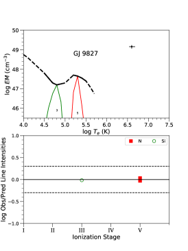
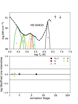
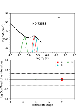
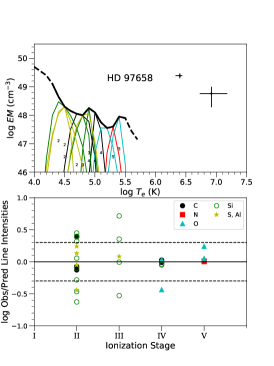
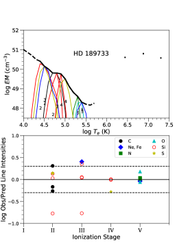
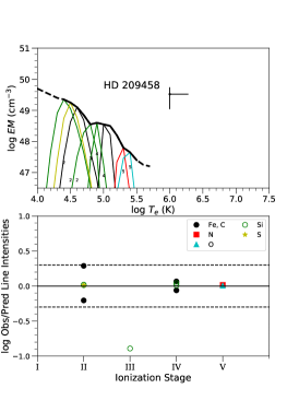
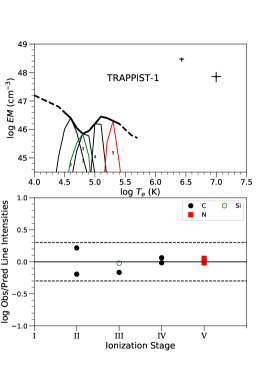
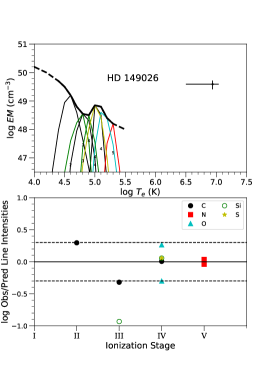
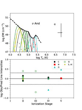
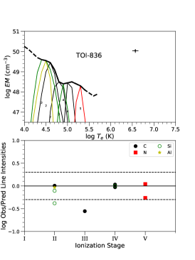
| Ion | (Å) | Ratio | Blends | |||
|---|---|---|---|---|---|---|
| S xv | 5.0387 | 7.3 | 2.51e14 | 3.1 | 0.46 | |
| Si xiv | 6.1804 | 7.3 | 6.55e14 | 9.3 | 0.29 | Si xiv 6.1858 |
| Si xiii | 6.6479 | 7.1 | 9.67e14 | 12.2 | 0.39 | |
| Si xii | 6.6638 | 7.0 | 1.06e14 | 4.1 | 0.01 | Si xii 6.6627 |
| Si xiii | 6.6882 | 7.1 | 2.19e14 | 5.8 | 0.35 | Si xiii 6.6850 |
| Si xiii | 6.7403 | 7.1 | 6.40e14 | 10.7 | 0.33 | Si xii 6.7432 |
| Mg xi | 7.4730 | 6.9 | 5.61e15 | 3.3 | 0.12 | Fe xxiii 7.4780 |
| Al xii | 7.7573 | 7.0 | 4.98e15 | 3.2 | 0.16 | |
| Mg xi | 7.8503 | 6.9 | 5.57e15 | 3.4 | 0.20 | |
| Fe xxiv | 7.9857 | 7.4 | 7.43e15 | 4.1 | 0.37 | Fe xxiii 7.9360, Fe xxiv 7.9960 |
| Fe xxiv | 8.3161 | 7.4 | 4.90e15 | 3.3 | 0.06 | Fe xxi 8.3162, Fe xxiii 8.3038 |
| Mg xii | 8.4192 | 7.1 | 4.70e14 | 10.4 | 0.18 | Mg xii 8.4246 |
| No id. | 8.4577 | 0.0 | 4.31e15 | 3.1 | … | |
| Fe xxii | 8.7140 | 7.2 | 6.13e15 | 3.7 | 0.11 | Fe xxii 8.7035, 8.7360, Ni xxii 8.7227, Ni xx 8.7286, Ni xix 8.7440 |
| Fe xxii | 8.9748 | 7.2 | 7.35e15 | 3.9 | 0.24 | |
| Fe xx | 9.0659 | 7.1 | 6.48e15 | 3.3 | 0.16 | Fe xxii 9.0501, 9.0629, Ni xxvi 9.0603, Fe xx 9.0647, 9.0683 |
| Mg xi | 9.1687 | 6.9 | 4.75e14 | 8.0 | 0.09 | |
| Mg xi | 9.2312 | 6.9 | 1.11e14 | 3.8 | 0.07 | Mg xi 9.2282, Fe xxii 9.2298 |
| Ni xix | 9.2540 | 7.0 | 7.66e15 | 3.2 | 0.19 | Ne x 9.2461, 9.2462 |
| Mg xi | 9.3143 | 6.9 | 2.35e14 | 5.6 | 0.13 | |
| Ni xx | 9.3850 | 7.1 | 4.77e15 | 3.4 | 0.51 | Ni xxvi 9.3853, Ni xxv 9.3900 |
| No id. | 9.4000 | 0.0 | 5.99e15 | 3.7 | … | |
| Ne x | 9.4807 | 6.9 | 1.56e14 | 5.8 | 0.02 | Ni xx 9.4719, Ne x 9.4809 |
| Ne x | 9.7080 | 6.9 | 2.09e14 | 5.4 | 0.16 | Ne x 9.7085 |
| Ni xix | 9.9770 | 7.0 | 8.01e15 | 3.6 | 0.05 | Ni xxv 9.9700, Fe xxi 9.9887 |
| No id. | 10.0100 | 0.0 | 9.21e15 | 3.8 | … | |
| Na xi | 10.0232 | 7.0 | 8.56e15 | 3.7 | 0.00 | Fe xx 10.0235, Na xi 10.0286 |
| No id. | 10.0500 | 0.0 | 6.03e15 | 3.1 | … | |
| Ni xix | 10.1100 | 7.0 | 6.34e15 | 3.2 | 0.15 | |
| Fe xvii | 10.1210 | 6.9 | 7.94e15 | 3.5 | 0.54 | Fe xix 10.1195, 10.1309 |
| Ne x | 10.2385 | 6.9 | 8.39e14 | 11.0 | 0.02 | Ne x 10.2396 |
| Fe xviii | 10.4483 | 7.0 | 1.39e14 | 4.4 | 0.26 | Fe xx 10.4537, Fe xviii 10.4639, 10.4654, 10.4726 |
| Fe xvii | 10.5040 | 6.9 | 1.32e14 | 4.2 | 0.34 | |
| Fe xviii | 10.5364 | 7.0 | 7.42e15 | 3.1 | 0.07 | Fe xviii 10.5382 |
| Fe xxiv | 10.6190 | 7.4 | 1.29e14 | 4.2 | 0.11 | Fe xix 10.6193 |
| Fe xvii | 10.7700 | 6.9 | 2.85e14 | 6.2 | 0.23 | Fe xix 10.7650, Ne ix 10.7650 |
| Fe xix | 10.8160 | 7.1 | 7.02e15 | 3.1 | 0.20 | Fe xix 10.8083 |
| Fe xxiii | 10.9810 | 7.3 | 1.91e14 | 4.9 | 0.08 | Fe xx 10.9866 |
| Ne ix | 11.0010 | 6.7 | 1.26e14 | 4.0 | 0.08 | Fe xx 11.0065 |
| Fe xxiv | 11.0290 | 7.4 | 1.62e14 | 4.5 | 0.06 | Fe xxiii 11.0190, Fe xvii 11.0260 |
| Fe xvii | 11.1310 | 6.9 | 2.13e14 | 5.0 | 0.10 | Fe xx 11.1415 |
| Fe xxiv | 11.1760 | 7.4 | 1.43e14 | 3.9 | 0.04 | Fe xxiv 11.1870, Ni xxii 11.1950 |
| Fe xvii | 11.2540 | 6.9 | 2.17e14 | 4.9 | 0.02 | |
| Fe xviii | 11.3260 | 7.0 | 2.40e14 | 5.1 | 0.07 | Fe xviii 11.3260, Ni xxi 11.3180, Fe xxiii 11.3360 |
| Fe xviii | 11.4230 | 7.0 | 1.71e14 | 4.2 | 0.27 | Fe xxii 11.4270, Fe xviii 11.4274, Fe xxiv 11.4320 |
| Fe xxiii | 11.4580 | 7.3 | 9.10e15 | 3.0 | 0.18 | Fe xviii 11.4445, 11.4471, Fe xxi 11.4451 |
| Fe xxii | 11.4900 | 7.2 | 9.37e15 | 3.2 | 0.12 | Fe xxii 11.4900, 11.5025 |
| Fe xviii | 11.5270 | 7.0 | 1.79e14 | 4.3 | 0.07 | Fe xviii 11.5270 |
| Ne ix | 11.5440 | 6.7 | 5.29e14 | 7.5 | 0.10 | Ni xix 11.5390 |
| No id. | 11.6060 | 0.0 | 1.06e14 | 3.4 | … | |
| Fe xxiii | 11.7360 | 7.3 | 3.01e14 | 5.5 | 0.02 | |
| Fe xxii | 11.7700 | 7.2 | 1.83e14 | 4.3 | 0.25 | Fe xx 11.7620 |
| Fe xxii | 11.9320 | 7.2 | 1.36e14 | 3.7 | 0.22 | Fe xxi 11.9432, Fe xxii 11.9474 |
| Ni xx | 12.1120 | 7.1 | 1.03e14 | 3.1 | 0.34 | Ne ix 12.1110, Fe xxi 12.1147 |
| Ne x | 12.1321 | 6.9 | 6.32e13 | 24.4 | 0.03 | Fe xvii 12.1240, Ne x 12.1375 |
| Fe xxiii | 12.1610 | 7.3 | 2.10e14 | 4.4 | 0.17 | |
| Fe xxii | 12.2100 | 7.2 | 1.12e14 | 3.2 | 0.11 | Fe xxii 12.2008, Fe xxi 12.2040, Ni xxi 12.2080, Fe xix 12.2120 |
| Fe xvii | 12.2660 | 6.9 | 3.58e14 | 5.7 | 0.09 | |
| Fe xxi | 12.2840 | 7.2 | 3.22e14 | 5.4 | 0.25 | |
| Ne ix | 12.3560 | 6.8 | 1.30e14 | 3.4 | 0.12 | Fe xxi 12.3508, 12.3527, 12.3626, 12.3628, 12.3630, Fe xxii 12.3648 |
| Fe xxi | 12.3930 | 7.2 | 1.18e14 | 3.2 | 0.07 | |
| Ni xix | 12.4350 | 7.0 | 2.16e14 | 4.4 | 0.39 | Fe xxi 12.4220, Fe xx 12.4234, 12.4310 |
| Fe xx | 12.4680 | 7.1 | 1.25e14 | 3.3 | 0.05 | Ni xviii 12.4590, Fe xxi 12.4625, Fe xxii 12.4728, Fe xix 12.4729, 12.4767 |
| Fe xxi | 12.4990 | 7.2 | 1.16e14 | 3.2 | 0.01 | Fe xxi 12.5023, 12.5048, Ni xxi 12.5105 |
| Fe xx | 12.5760 | 7.1 | 1.40e14 | 3.5 | 0.14 | |
| Ni xix | 12.6560 | 7.0 | 1.29e14 | 3.3 | 0.02 | Fe xxi 12.6490 |
| Ni xix | 12.8120 | 7.0 | 1.49e14 | 3.5 | 0.29 | Fe xxi 12.8071, 12.8089, 12.8095, 12.8110, Mn xxii 12.8109 |
| Fe xx | 12.8240 | 7.1 | 1.02e13 | 9.1 | 0.01 | Fe xxi 12.8220, Fe xx 12.8460 |
| Fe xx | 12.9120 | 7.1 | 1.15e14 | 3.0 | 0.22 | Fe xix 12.9033, 12.9169 |
| Fe xx | 12.9650 | 7.1 | 2.16e14 | 4.1 | 0.15 | Fe xviii 12.9494, Fe xxii 12.9530 |
| Fe xix | 13.0220 | 7.1 | 1.73e14 | 3.7 | 0.00 | Fe xviii 13.0121, Fe xxi 13.0126, Fe xx 13.0152, 13.0240 |
| Fe xx | 13.1000 | 7.1 | 2.49e14 | 4.1 | 0.46 | Fe xix 13.0810, 13.1011, Fe xxi 13.1056 |
| Fe xx | 13.1370 | 7.1 | 1.87e14 | 3.6 | 0.28 | Fe xxi 13.1223, 13.1338, Ni xx 13.1350 |
| Fe xx | 13.1530 | 7.1 | 1.74e14 | 3.5 | 0.07 | Fe xvii 13.1530, Fe xx 13.1565, Ni xx 13.1610 |
| Fe xviii | 13.3230 | 7.0 | 1.56e14 | 3.3 | 0.02 | Ni xx 13.3090, 13.3236, Fe xviii 13.3312 |
| Fe xx | 13.3850 | 7.1 | 1.68e14 | 3.3 | 0.16 | Fe xviii 13.3550, 13.3807, Fe xx 13.3752, 13.3953 |
| Fe xix | 13.4230 | 7.1 | 2.32e14 | 3.8 | 0.42 | Fe xix 13.4239 |
| Ne ix | 13.4473 | 6.7 | 4.13e13 | 16.2 | 0.26 | |
| Fe xix | 13.4620 | 7.1 | 4.72e14 | 5.6 | 0.18 | Ne viii 13.4610, 13.4690, 13.4700 |
| Fe xix | 13.4970 | 7.1 | 2.27e14 | 3.9 | 0.24 | Ne viii 13.4910, Fe xix 13.4923 |
| Fe xix | 13.5180 | 7.1 | 7.87e14 | 7.3 | 0.01 |
| Ion | (Å) | Ratio | Blends | |||
|---|---|---|---|---|---|---|
| Ne ix | 13.5531 | 6.7 | 5.60e14 | 6.2 | 0.08 | |
| Fe xix | 13.6450 | 7.1 | 2.21e14 | 3.7 | 0.22 | Fe xix 13.6442, 13.6476 |
| Ne ix | 13.6990 | 6.7 | 2.50e13 | 12.5 | 0.24 | Fe xix 13.6878, 13.7054 |
| Fe xix | 13.7590 | 7.1 | 2.39e14 | 3.6 | 0.42 | |
| Ni xix | 13.7790 | 7.0 | 2.05e14 | 3.3 | 0.07 | Fe xx 13.7670, Fe xix 13.8041, 13.8068 |
| Fe xix | 13.7950 | 7.1 | 2.86e14 | 3.8 | 0.04 | |
| Fe xvii | 13.8250 | 6.9 | 2.03e14 | 3.1 | 0.17 | |
| Fe xix | 13.8390 | 7.1 | 1.95e14 | 3.0 | 0.27 | Fe xx 13.8430 |
| Fe xviii | 13.9530 | 7.0 | 4.66e14 | 4.5 | 0.39 | Fe xix 13.9263, 13.9330, Fe xx 13.9620 |
| Ni xix | 14.0430 | 7.0 | 2.29e14 | 3.5 | 0.21 | Fe xix 14.0179, 14.0340, 14.0388 |
| Ni xix | 14.0770 | 7.0 | 2.94e14 | 3.9 | 0.13 | Fe xix 14.0610, Fe xx 14.0620, 14.0784 |
| No id. | 14.1736 | 0.0 | 1.59e14 | 3.0 | … | |
| Fe xviii | 14.2080 | 7.0 | 1.03e13 | 7.8 | 0.25 | |
| No id. | 14.2492 | 0.0 | 2.71e14 | 4.0 | … | |
| Fe xviii | 14.2560 | 7.0 | 3.51e14 | 4.6 | 0.12 | Fe xx 14.2670 |
| Fe xx | 14.3259 | 7.1 | 1.53e14 | 3.3 | 0.78 | Fe xix 14.3275, 14.3391, 14.3397, Fe xx 14.3321, Fe xxi 14.3388 |
| Fe xviii | 14.3430 | 7.0 | 1.89e14 | 3.7 | 0.06 | |
| Fe xviii | 14.3730 | 7.0 | 3.01e14 | 4.7 | 0.16 | |
| Fe xviii | 14.4250 | 7.0 | 1.68e14 | 3.5 | 0.17 | Fe xix 14.4106 |
| Fe xviii | 14.4345 | 7.0 | 1.81e14 | 3.6 | 0.31 | Fe xviii 14.4432 |
| Fe xx | 14.4600 | 7.1 | 2.92e14 | 4.6 | 0.14 | Fe xviii 14.4610, 14.4555, 14.4769, Fe xx 14.4793 |
| Fe xviii | 14.5340 | 7.0 | 7.96e14 | 7.4 | 0.03 | O viii 14.5242, 14.5243, Fe xviii 14.5608, 14.5710 |
| O viii | 14.6342 | 6.6 | 1.56e14 | 3.2 | 0.12 | O viii 14.6344 |
| Fe xix | 14.6640 | 7.1 | 2.12e14 | 3.7 | 0.01 | |
| Fe xx | 14.7540 | 7.1 | 1.80e14 | 3.5 | 0.12 | Fe xviii 14.7499, 14.7510 |
| O viii | 14.8205 | 6.6 | 3.20e14 | 4.5 | 0.11 | O viii 14.8207, Fe xx 14.8304 |
| Fe xvii | 15.0140 | 6.9 | 3.77e13 | 14.5 | 0.04 | |
| Fe xvi | 15.0496 | 6.7 | 3.54e14 | 4.5 | 0.31 | Fe xx 15.0470, 15.0470 |
| Fe xix | 15.0790 | 7.1 | 3.48e14 | 4.5 | 0.12 | |
| O viii | 15.1760 | 6.6 | 7.73e14 | 6.4 | 0.08 | O viii 15.1765, Fe xix 15.1770 |
| Fe xix | 15.1980 | 7.1 | 3.25e14 | 4.1 | 0.27 | Fe xviii 15.1898 |
| Fe xvii | 15.2610 | 6.9 | 1.77e13 | 9.5 | 0.21 | |
| Fe xvii | 15.4530 | 6.8 | 2.87e14 | 3.9 | 0.23 | |
| Fe xviii | 15.4940 | 7.0 | 1.78e14 | 3.1 | 0.32 | Fe xvi 15.4955, 15.5023, Cr xviii 15.5020 |
| Fe xviii | 15.6250 | 7.0 | 3.51e14 | 4.4 | 0.17 | |
| Fe xviii | 15.8240 | 7.0 | 3.53e14 | 4.4 | 0.05 | |
| Fe xviii | 15.8700 | 7.0 | 2.36e14 | 3.6 | 0.04 | Fe xix 15.8708 |
| O viii | 16.0055 | 6.6 | 2.61e13 | 11.6 | 0.02 | Fe xviii 16.0040, O viii 16.0067 |
| Fe xviii | 16.0710 | 7.0 | 1.10e13 | 7.5 | 0.09 | |
| No id. | 16.7276 | 0.0 | 2.07e14 | 3.0 | … | |
| Fe xvii | 16.7800 | 6.8 | 2.38e13 | 10.1 | 0.04 | |
| Fe xvii | 17.0510 | 6.8 | 3.27e13 | 11.4 | 0.10 | |
| Fe xvii | 17.0960 | 6.8 | 2.56e13 | 10.0 | 0.11 | |
| Fe xviii | 17.6230 | 7.0 | 2.73e14 | 3.1 | 0.24 | |
| O vii | 18.6270 | 6.4 | 7.76e14 | 4.9 | 0.03 | Ar xvi 18.6324 |
| O viii | 18.9671 | 6.6 | 1.38e12 | 19.0 | 0.01 | O viii 18.9725 |
| O vii | 21.6015 | 6.4 | 4.51e13 | 8.1 | 0.00 | |
| O vii | 21.8036 | 6.4 | 1.12e13 | 3.8 | 0.08 | |
| O vii | 22.0977 | 6.4 | 1.93e13 | 4.7 | 0.19 | |
| N vii | 24.7792 | 6.4 | 1.51e13 | 4.6 | 0.25 | N vii 24.7846 |
| C vi | 28.4652 | 6.3 | 3.96e14 | 6.5 | 0.18 | C vi 28.4663 |
| N vi | 28.7870 | 6.3 | 3.67e14 | 6.2 | 0.19 | |
| N vi | 29.0843 | 6.2 | 3.27e14 | 5.8 | 0.38 | |
| N vi | 29.5347 | 6.2 | 3.86e14 | 6.2 | 0.01 | Si xii 29.5090 |
| S xiv | 30.4270 | 6.6 | 3.65e14 | 5.6 | 0.12 | |
| S xiv | 30.4690 | 6.6 | 1.52e14 | 3.7 | 0.04 | |
| S xiii | 32.2391 | 6.6 | 2.90e14 | 5.5 | 0.39 | S xiii 32.1911 |
| S xiv | 32.5600 | 6.6 | 4.60e14 | 6.9 | 0.09 | S xiv 32.5750 |
| S xiv | 33.5490 | 6.6 | 4.68e14 | 6.9 | 0.36 | Si xi 33.5301 |
| C vi | 33.7342 | 6.2 | 2.61e13 | 16.3 | 0.21 | C vi 33.7396 |
| Si xi | 43.7501 | 6.4 | 2.34e14 | 7.8 | 0.03 | |
| Si xii | 44.0190 | 6.4 | 3.07e14 | 9.1 | 0.01 | |
| Si xii | 44.1650 | 6.4 | 5.73e14 | 12.4 | 0.03 | |
| Si xii | 45.5210 | 6.4 | 2.44e14 | 8.1 | 0.24 | |
| Si xii | 45.6910 | 6.4 | 2.58e14 | 8.4 | 0.03 | |
| Fe xvi | 50.3613 | 6.6 | 8.09e15 | 4.3 | 0.00 | |
| Fe xvi | 54.1264 | 6.6 | 1.46e14 | 4.2 | 0.12 | S viii 54.1181, S ix 54.1750 |
| Fe xvi | 54.7101 | 6.6 | 1.98e14 | 4.9 | 0.21 | Fe xvi 54.7472 |
| Mg x | 57.8760 | 6.2 | 8.36e15 | 4.2 | 0.15 | |
| Fe xvi | 63.7106 | 6.6 | 8.70e15 | 3.0 | 0.22 | |
| Mg x | 65.8450 | 6.2 | 1.59e14 | 5.3 | 0.48 | Ne viii 65.8940 |
| Fe xvi | 66.3568 | 6.6 | 4.83e14 | 9.7 | 0.36 | Fe xvi 66.2489 |
| Ne viii | 88.0820 | 5.9 | 3.59e14 | 13.2 | 0.24 | Ne viii 88.1190 |
| Fe xii | 89.8267 | 6.3 | 1.40e14 | 7.3 | 0.39 | Fe xii 89.4789, Fe xvii 89.5977, Ne vii 89.9472 |
| Fe xix | 91.0200 | 7.0 | 1.77e14 | 8.4 | 0.06 | Fe xvii 90.5205, Fe xx 90.6000, Fe x 90.6830, Fe xiii 90.7058, Fe xi 90.7197 |
| Fe xiv | 92.4616 | 6.4 | 7.45e15 | 4.3 | 0.17 | Fe xvii 92.0282, Fe xiv 92.0572, Fe xi 92.7554 |
| Fe xviii | 93.9230 | 7.0 | 7.72e14 | 23.2 | 0.07 | |
| Ne viii | 98.2600 | 5.9 | 6.45e14 | 20.9 | 0.19 | Fe xxi 97.8800, Ne viii 98.1150 |
| Fe xix | 101.5500 | 7.0 | 1.17e14 | 6.7 | 0.37 | |
| Fe xxi | 102.2200 | 7.2 | 3.05e14 | 14.0 | 0.14 | Fe xiii 102.0757, O viii 102.3476, 102.3552, 102.3919, 102.4897, 102.5497 |
| Ne viii | 103.0850 | 5.9 | 1.57e14 | 8.9 | 0.14 | Ni xxii 103.3260, Fe xiii 103.3386 |
| Fe xviii | 103.9370 | 7.0 | 2.27e14 | 11.3 | 0.12 | |
| O vi | 104.8130 | 5.6 | 7.03e15 | 5.9 | 0.55 | O vi 104.8129, Fe xvii 104.7669 |
| Ion | (Å) | Ratio | Blends | |||
|---|---|---|---|---|---|---|
| Ni xxii | 106.0640 | 7.2 | 7.74e15 | 6.0 | 0.02 | Fe xii 106.0264, 106.0341, 106.2027, Fe xix 106.1200, 106.3300 |
| Fe xix | 108.3700 | 7.0 | 5.02e14 | 19.4 | 0.16 | |
| Fe xix | 109.9700 | 7.0 | 6.86e15 | 5.7 | 0.27 | |
| Fe xx | 110.6300 | 7.1 | 6.43e15 | 4.5 | 0.09 | Fe xx 110.4464 |
| Fe xix | 111.7000 | 7.0 | 8.00e15 | 5.2 | 0.20 | Ni xxiii 111.8600 |
| Fe xxii | 114.4100 | 7.2 | 1.32e14 | 7.8 | 0.10 | Fe xii 114.5616, 114.9055 |
| Mn xviii | 115.3653 | 7.0 | 1.04e14 | 7.2 | 0.09 | |
| Fe xxii | 117.1700 | 7.2 | 5.58e14 | 19.6 | 0.01 | Fe xxi 117.5100 |
| Ni xxv | 117.9330 | 7.4 | 7.41e15 | 5.7 | 0.04 | Ni xxii 117.9330, Cr xx 117.9580 |
| Fe xx | 118.6600 | 7.1 | 1.49e14 | 8.5 | 0.18 | |
| Fe xix | 120.0000 | 7.0 | 1.51e14 | 8.0 | 0.22 | O vii 120.3310, O vii 120.3327 |
| Fe xx | 121.8300 | 7.1 | 3.60e14 | 14.1 | 0.08 | |
| Ne vi | 122.4879 | 5.8 | 6.45e15 | 4.5 | 0.08 | Ne vi 122.6850, Cr xvii 122.9718 |
| Fe xxi | 128.7300 | 7.2 | 5.59e14 | 17.2 | 0.00 | |
| Fe xxiii | 132.8500 | 7.3 | 1.65e13 | 30.6 | 0.04 | Fe xx 132.8500 |
| Fe xxii | 135.7800 | 7.2 | 4.26e14 | 14.3 | 0.02 | |
| Fe xxi | 142.2700 | 7.2 | 1.87e14 | 8.1 | 0.28 | Fe xxi 142.1600 |
| Fe ix | 171.0729 | 6.0 | 5.97e14 | 9.9 | 0.10 | Ni xiv 171.3703 |
| Fe x | 174.5310 | 6.1 | 6.07e14 | 8.6 | 0.00 | |
| Fe xi | 180.4080 | 6.2 | 2.41e14 | 6.1 | 0.69 | |
| Fe xii | 193.5090 | 6.3 | 2.02e13 | 19.1 | 0.28 | S xi 191.2664, Fe xxiv 192.0170, Fe xii 192.3940, 195.1190 |
| Fe xiii | 203.8280 | 6.3 | 5.00e14 | 9.2 | 0.23 | Ar xiv 203.3510, Fe xii 203.7280, Mn xi 203.9122, Fe xi 204.7440, Fe xiii 204.9450 |
| Fe xiv | 211.3180 | 6.4 | 6.67e14 | 10.2 | 0.28 | |
| Ni xvii | 249.1780 | 6.6 | 5.20e14 | 7.1 | 0.30 | Fe xii 248.7670, 249.3880 |
| Fe xv | 284.1630 | 6.4 | 2.38e13 | 15.4 | 0.13 | |
| Fe xvi | 335.4098 | 6.5 | 2.59e13 | 12.7 | 0.04 | Fe xiv 334.1800 |
| Fe xvi | 360.7581 | 6.5 | 1.09e13 | 6.6 | 0.07 | Fe xiii 359.6420, 359.8420 |
| C iii | 1176.0000 | 4.8 | 1.93e13 | 20.4 | 0.06 | |
| S iii | 1190.1990 | 4.9 | 9.87e16 | 8.2 | 0.64 | |
| S iii | 1194.0490 | 4.9 | 2.21e15 | 10.7 | 0.19 | |
| Si ii | 1194.5010 | 4.6 | 3.38e15 | 13.6 | 0.27 | S iii 1194.4430 |
| Si ii | 1197.3950 | 4.6 | 2.14e15 | 27.6 | 0.00 | |
| S v | 1199.1360 | 5.3 | 2.13e15 | 9.1 | 0.04 | |
| S iii | 1200.9610 | 4.9 | 4.52e15 | 23.4 | 0.16 | |
| O ii | 1204.2345 | 4.9 | 5.35e16 | 4.9 | 0.19 | |
| Si iii | 1206.5019 | 4.9 | 1.29e13 | 56.2 | 0.29 | |
| O v | 1218.3440 | 5.5 | 2.63e14 | 78.3 | 0.13 | |
| N v | 1238.8218 | 5.4 | 9.23e14 | 79.2 | 0.12 | |
| Fe xii | 1242.0050 | 6.3 | 2.28e15 | 25.8 | 0.38 | |
| N v | 1242.8042 | 5.4 | 4.50e14 | 41.2 | 0.11 | |
| C iii | 1247.3830 | 5.1 | 1.88e15 | 17.6 | 0.24 | |
| Ne ix | 1248.1030 | 6.7 | 6.81e16 | 32.1 | 0.03 | |
| S ii | 1250.5870 | 4.6 | 1.05e15 | 22.1 | 0.05 | |
| S ii | 1253.8130 | 4.6 | 1.69e15 | 19.9 | 0.15 | |
| S ii | 1259.5210 | 4.6 | 2.40e15 | 31.8 | 0.22 | |
| Si ii | 1264.7400 | 4.5 | 7.76e15 | 24.2 | 0.31 | |
| Si ii | 1265.0040 | 4.6 | 3.82e15 | 19.5 | 0.19 | |
| Si ii | 1304.3719 | 4.6 | 2.89e15 | 21.5 | 0.33 | |
| Si ii | 1309.2770 | 4.6 | 5.77e15 | 35.4 | 0.33 | |
| Si iii | 1312.5930 | 4.9 | 8.90e16 | 14.3 | 0.47 | |
| C ii | 1323.9080 | 4.8 | 2.22e15 | 18.3 | 0.39 | |
| Fe xix | 1328.6999 | 7.1 | 1.82e15 | 13.8 | 0.08 | |
| C ii | 1334.5350 | 4.7 | 5.16e14 | 41.6 | 0.29 | |
| C ii | 1335.7100 | 4.7 | 1.59e13 | 64.2 | 0.54 | |
| O iv | 1338.6140 | 5.3 | 4.70e16 | 13.4 | 0.02 | |
| Fe xii | 1349.4000 | 6.3 | 8.71e16 | 16.8 | 0.20 | |
| Fe xxi | 1354.0800 | 7.2 | 7.30e15 | 12.5 | 0.08 | |
| O v | 1371.2960 | 5.5 | 5.97e15 | 25.3 | 0.16 | |
| Ar xi | 1392.0980 | 6.4 | 1.10e15 | 24.2 | 0.02 | |
| Si iv | 1393.7552 | 5.0 | 1.09e13 | 52.0 | 0.19 | |
| Si iv | 1402.7704 | 5.0 | 6.32e14 | 35.6 | 0.25 | |
| Si iii | 1417.2400 | 4.9 | 8.94e16 | 23.1 | 0.34 | |
| Si viii | 1445.7371 | 6.0 | 4.82e16 | 9.1 | 0.20 | |
| S v | 1501.7660 | 5.3 | 1.19e15 | 19.5 | 0.19 | |
| Si ii | 1526.7090 | 4.5 | 8.05e15 | 21.8 | 0.33 | |
| Si ii | 1533.4320 | 4.5 | 1.40e14 | 20.5 | 0.28 | |
| C iv | 1548.1871 | 5.1 | 3.54e13 | 64.5 | 0.09 | |
| C iv | 1550.7723 | 5.1 | 1.93e13 | 48.7 | 0.05 | |
| Ne v | 1574.7560 | 5.5 | 1.31e15 | 15.2 | 0.36 | |
| S xi | 1614.4946 | 6.4 | 1.23e15 | 8.8 | 0.27 | |
| O vii | 1623.6672 | 6.4 | 2.41e15 | 12.4 | 0.08 | |
| S iv | 1629.1550 | 5.2 | 1.03e15 | 10.7 | 0.33 | |
| Al ii | 1670.7870 | 4.6 | 1.52e14 | 17.9 | 0.22 |
| Ion | (Å) | Ratio | Blends | |||
|---|---|---|---|---|---|---|
| Si xiv | 6.1804 | 7.3 | 2.47e14 | 3.8 | 0.02 | Si xiv 6.1858 |
| Ne x | 10.2385 | 6.9 | 5.38e15 | 3.9 | 0.20 | Ne x 10.2396 |
| No id. | 10.5040 | 0.0 | 5.56e15 | 4.0 | … | |
| No id. | 10.7700 | 0.0 | 6.84e15 | 4.6 | … | |
| Ne ix | 11.5440 | 6.7 | 4.38e15 | 3.9 | 0.16 | Fe xxii 11.4900, Fe xviii 11.5270 |
| Ne x | 12.1321 | 6.9 | 1.92e14 | 8.5 | 0.10 | Fe xvii 12.1240, Ne x 12.1375 |
| Fe xvi | 12.5399 | 6.8 | 2.64e15 | 3.2 | 0.29 | Fe xxi 12.4990, 12.5048, Fe xx 12.5260, 12.5760, Fe xvii 12.5391 |
| Ne ix | 13.4473 | 6.7 | 3.23e14 | 11.8 | 0.21 | Fe xix 13.4970, 13.5180, Ne ix 13.5531 |
| Ne ix | 13.6990 | 6.7 | 5.52e15 | 4.1 | 0.13 | Fe xix 13.6450, 13.7054 |
| Fe xvii | 13.8250 | 6.9 | 7.16e15 | 5.6 | 0.26 | Fe xix 13.7590, 13.7950, 13.8390, Fe xx 13.7670, Ni xix 13.7790, Fe xvii 13.8920 |
| Fe xviii | 14.2080 | 7.0 | 4.78e15 | 4.7 | 0.24 | Fe xviii 14.2560, Fe xx 14.2670 |
| Fe xviii | 14.3730 | 7.0 | 5.79e15 | 5.1 | 0.14 | Fe xviii 14.3430, 14.3990, 14.4250, 14.4555 |
| Fe xviii | 14.5340 | 7.0 | 2.17e15 | 3.1 | 0.12 | O viii 14.5242, 14.5243, Fe xviii 14.5608, 14.5710 |
| Fe xvi | 14.9555 | 6.7 | 3.70e15 | 4.1 | 0.08 | O viii 14.8205, 14.8207, Fe xix 14.9610 |
| Fe xvii | 15.0140 | 6.9 | 1.50e14 | 8.3 | 0.02 | |
| O viii | 15.1760 | 6.6 | 3.15e15 | 3.8 | 0.20 | O viii 15.1765, Fe xix 15.1980 |
| Fe xvii | 15.2610 | 6.9 | 4.38e15 | 4.5 | 0.02 | |
| Fe xvii | 15.4530 | 6.8 | 3.60e15 | 4.1 | 0.41 | Fe xvi 15.4485, 15.4533, 15.5023, Fe xviii 15.4940, Fe xx 15.5170 |
| O viii | 16.0055 | 6.6 | 1.60e14 | 8.4 | 0.07 | Fe xviii 16.0040, O viii 16.0067 |
| Fe xix | 16.2830 | 7.1 | 3.24e15 | 3.9 | 0.36 | Fe xvii 16.2285, 16.3500, Fe xix 16.2857, 16.3247, Fe xviii 16.3200 |
| Fe xvii | 16.7800 | 6.8 | 1.11e14 | 7.2 | 0.11 | |
| Fe xvii | 17.0510 | 6.8 | 1.59e14 | 8.5 | 0.13 | Fe xvii 17.0960 |
| Fe xviii | 17.6230 | 7.0 | 1.86e15 | 3.0 | 0.03 | |
| O vii | 18.6270 | 6.4 | 6.27e15 | 5.5 | 0.14 | Ar xvi 18.6324, Ca xviii 18.6909 |
| O viii | 18.9671 | 6.6 | 6.88e14 | 18.1 | 0.01 | O viii 18.9725 |
| O vii | 21.6015 | 6.4 | 3.61e14 | 12.3 | 0.19 | |
| O vii | 21.8036 | 6.4 | 2.41e15 | 3.2 | 0.16 | |
| O vii | 22.0977 | 6.4 | 2.38e14 | 9.9 | 0.18 | |
| No id. | 23.0050 | 0.0 | 4.01e15 | 3.6 | … | |
| N vii | 24.7792 | 6.4 | 5.49e15 | 5.1 | 0.28 | Ar xv 24.7366, 24.7400, N vii 24.7846, Ar xvi 24.8509 |
| C vi | 26.9896 | 6.3 | 2.88e15 | 3.5 | 0.21 | C vi 26.9901, Ar xv 27.0432 |
| Ar xiv | 27.4640 | 6.7 | 3.11e15 | 3.6 | 0.17 | Ar xiv 27.6310, 27.6360 |
| Ar xiii | 29.1420 | 6.6 | 4.95e15 | 4.2 | 0.10 | |
| S xiv | 30.4270 | 6.6 | 3.88e15 | 3.5 | 0.09 | Ca xi 30.4480, S xiv 30.4690 |
| S xiv | 32.5600 | 6.6 | 4.02e15 | 3.4 | 0.06 | S xiv 32.5750, Ca xii 32.6571 |
| C vi | 33.7342 | 6.2 | 3.44e14 | 10.0 | 0.23 | C vi 33.7396 |
| No id. | 35.6844 | 0.0 | 5.70e15 | 3.8 | … | |
| O v | 1218.3440 | 5.5 | 2.51e15 | 4.4 | 0.06 | |
| N v | 1238.8218 | 5.4 | 2.55e15 | 4.1 | 0.14 | |
| N v | 1242.8042 | 5.4 | 1.47e15 | 3.0 | 0.20 | |
| Si ii | 1264.7400 | 4.5 | 3.90e16 | 4.2 | 0.06 | |
| C ii | 1335.7100 | 4.7 | 4.12e15 | 5.6 | 0.22 | C ii 1335.6650 |
| O v | 1371.2960 | 5.5 | 2.96e16 | 3.4 | 0.28 | |
| Si iv | 1393.7552 | 5.0 | 4.73e15 | 5.2 | 0.02 | |
| O iv | 1401.1570 | 5.3 | 5.89e16 | 3.0 | 0.48 | |
| Si iv | 1402.7704 | 5.0 | 1.61e15 | 5.4 | 0.15 | |
| Si ii | 1533.4320 | 4.5 | 4.96e16 | 3.2 | 0.06 | |
| C iv | 1548.1871 | 5.1 | 1.66e14 | 8.1 | 0.00 | |
| C iv | 1550.7723 | 5.1 | 7.85e15 | 5.6 | 0.03 | |
| Al ii | 1670.7870 | 4.6 | 4.41e15 | 3.1 | 0.02 |
| Ion | (Å) | Ratio | Blends | |||
|---|---|---|---|---|---|---|
| Fe xxiii | 11.7360 | 7.3 | 2.86e15 | 3.1 | 0.39 | |
| Fe xxii | 11.9770 | 7.2 | 6.49e15 | 4.8 | 0.22 | Fe xxii 11.8810, 11.9320, 11.9474, Fe xxi 11.9023, 11.9750, Ni xx 11.9617 |
| Ne x | 12.1321 | 6.9 | 2.24e14 | 9.0 | 0.11 | Fe xvii 12.1240, Ne x 12.1375, Fe xxiii 12.1610 |
| Fe xxi | 12.2840 | 7.2 | 2.51e15 | 3.0 | 0.79 | Fe xvii 12.2660 |
| Ne ix | 13.4473 | 6.7 | 2.15e14 | 9.4 | 0.16 | Fe xix 13.4620, 13.4970, 13.5180, Fe xxi 13.5070 |
| Ne ix | 13.6990 | 6.7 | 1.93e14 | 9.0 | 0.41 | Fe xix 13.6450, 13.6878, 13.7054 |
| Fe xviii | 14.2080 | 7.0 | 1.01e14 | 6.5 | 0.33 | Fe xviii 14.2560, Fe xx 14.2670 |
| Fe xviii | 14.3730 | 7.0 | 3.14e15 | 3.6 | 0.55 | Fe xviii 14.3430, 14.3430, 14.3990, 14.4250, 14.4555, Fe xx 14.3887 |
| Fe xviii | 14.5340 | 7.0 | 6.56e15 | 5.3 | 0.02 | O viii 14.5242, Fe xviii 14.5608, 14.5710 |
| Fe xvi | 14.9555 | 6.7 | 4.92e15 | 4.6 | 0.26 | O viii 14.8205, 14.8207, Fe xx 14.8791, 14.9279, Fe xix 14.9610, 14.9632 |
| Fe xvii | 15.0140 | 6.9 | 1.69e14 | 8.6 | 0.11 | |
| Fe xix | 15.0790 | 7.1 | 7.77e15 | 5.8 | 0.38 | |
| O viii | 15.1760 | 6.6 | 5.02e15 | 4.6 | 0.17 | O viii 15.1765, Fe xix 15.1980 |
| Fe xvii | 15.2610 | 6.9 | 9.26e15 | 6.3 | 0.16 | |
| O viii | 16.0055 | 6.6 | 1.89e14 | 9.2 | 0.13 | Fe xviii 16.0040, 16.0710, O viii 16.0067 |
| Fe xvii | 16.7800 | 6.8 | 7.27e15 | 5.7 | 0.19 | |
| Fe xvii | 17.0510 | 6.8 | 3.35e14 | 12.2 | 0.08 | Fe xvii 17.0960 |
| O viii | 18.9671 | 6.6 | 9.82e14 | 20.8 | 0.15 | O viii 18.9725 |
| O vii | 21.6015 | 6.4 | 5.02e14 | 14.1 | 0.13 | |
| O vii | 21.8036 | 6.4 | 5.34e15 | 4.6 | 0.08 | |
| O vii | 22.0977 | 6.4 | 2.14e14 | 9.1 | 0.12 | |
| N vii | 24.7792 | 6.4 | 6.15e15 | 5.1 | 0.25 | N vii 24.7846, N vi 24.8980 |
| C vi | 33.7342 | 6.2 | 4.45e14 | 9.9 | 0.48 | C vi 33.7396 |
| Si iii | 1108.3610 | 4.9 | 1.13e15 | 3.8 | 0.20 | |
| Si iii | 1109.9720 | 4.9 | 2.22e15 | 5.3 | 0.13 | Si iii 1109.9430 |
| Si iii | 1113.2321 | 4.9 | 3.00e15 | 7.1 | 0.06 | Si iii 1113.2061 |
| Fe xix | 1118.0700 | 7.0 | 1.07e15 | 4.9 | 0.18 | |
| Si iv | 1122.4852 | 5.0 | 1.74e15 | 4.9 | 0.53 | |
| Si iv | 1128.3405 | 5.0 | 2.74e15 | 6.2 | 0.41 | Si iv 1128.3252 |
| Ne v | 1136.5081 | 5.5 | 2.01e16 | 3.6 | 0.02 | |
| Fe iii | 1141.7170 | 4.6 | 1.69e16 | 3.9 | 0.45 | |
| Ne v | 1145.5959 | 5.5 | 4.22e16 | 4.2 | 0.11 | |
| C iii | 1176.0000 | 4.8 | 5.24e14 | 21.6 | 0.01 | |
| C iii | 1176.0000 | 4.8 | 1.74e14 | 4.1 | 0.49 | |
| S iii | 1190.1990 | 4.9 | 4.99e16 | 8.4 | 0.36 | |
| Si ii | 1190.4170 | 4.6 | 4.62e16 | 6.5 | 0.30 | |
| Si ii | 1193.2910 | 4.6 | 4.15e16 | 6.7 | 0.53 | |
| S iii | 1194.4430 | 4.9 | 1.65e15 | 8.6 | 0.01 | S iii 1194.0490 |
| Si ii | 1197.3950 | 4.6 | 3.62e16 | 6.7 | 0.29 | |
| S v | 1199.1360 | 5.3 | 2.87e16 | 6.6 | 0.08 | |
| S iii | 1200.9611 | 4.9 | 1.41e15 | 12.8 | 0.22 | |
| S iii | 1201.7200 | 4.9 | 3.78e16 | 6.1 | 0.19 | |
| O ii | 1204.2345 | 4.9 | 3.66e16 | 9.5 | 0.04 | |
| Si iii | 1206.5019 | 4.9 | 3.15e14 | 33.6 | 0.68 | |
| N v | 1238.8218 | 5.4 | 1.51e14 | 24.4 | 0.09 | |
| Fe xii | 1242.0050 | 6.3 | 4.22e16 | 8.1 | 0.18 | |
| N v | 1242.8042 | 5.4 | 7.54e15 | 19.5 | 0.09 | |
| C iii | 1247.3830 | 5.1 | 1.08e15 | 10.9 | 0.24 | |
| S ii | 1250.5870 | 4.6 | 3.57e16 | 4.7 | 0.18 | |
| S ii | 1253.8130 | 4.6 | 4.03e16 | 4.8 | 0.07 | |
| S ii | 1259.5210 | 4.6 | 6.18e16 | 7.2 | 0.12 | |
| Si ii | 1260.4239 | 4.6 | 1.02e15 | 7.2 | 0.59 | |
| Si ii | 1264.7400 | 4.5 | 1.59e15 | 10.8 | 0.16 | |
| Si ii | 1265.0040 | 4.6 | 7.76e16 | 8.6 | 0.00 | |
| Si iii | 1303.3250 | 4.9 | 1.76e15 | 13.6 | 0.76 | |
| Si ii | 1304.3719 | 4.6 | 4.96e16 | 9.5 | 0.09 | |
| Si ii | 1309.2770 | 4.6 | 1.02e15 | 7.9 | 0.11 | |
| Si iii | 1312.5930 | 4.9 | 4.14e16 | 5.2 | 0.54 | |
| C ii | 1323.9080 | 4.8 | 6.49e16 | 6.0 | 0.02 | C ii 1323.8640, 1323.9540 |
| Fe xix | 1328.7000 | 7.1 | 2.69e16 | 5.2 | 0.03 | |
| C ii | 1334.5350 | 4.7 | 1.83e14 | 21.4 | 0.22 | |
| C ii | 1335.7100 | 4.7 | 2.98e14 | 27.4 | 0.19 | C ii 1335.6650 |
| O iv | 1338.6140 | 5.3 | 1.49e16 | 3.5 | 0.12 | |
| Fe xxi | 1354.0800 | 7.2 | 1.22e15 | 5.3 | 0.08 | |
| Si iv | 1393.7552 | 5.0 | 1.14e14 | 3.3 | 0.37 | |
| Si iv | 1402.7704 | 5.0 | 7.65e15 | 3.2 | 0.24 | |
| Si ii | 1526.7090 | 4.5 | 1.51e15 | 8.6 | 0.19 | |
| Si ii | 1533.4320 | 4.5 | 1.63e15 | 5.7 | 0.08 | |
| C iv | 1548.1871 | 5.1 | 3.53e14 | 4.7 | 0.20 | |
| C iv | 1550.7723 | 5.1 | 2.29e14 | 9.4 | 0.08 | |
| Al ii | 1670.7870 | 4.6 | 4.14e15 | 11.3 | 0.00 |
| Ion | 55 Cnc | HD 97658 | Barnard’s star | HD 189733 | And | |||||||||||||
|---|---|---|---|---|---|---|---|---|---|---|---|---|---|---|---|---|---|---|
| (Å) | (K) | Ratio | Ratio | Ratio | Ratio | Ratio | Blends | |||||||||||
| Si iii | 1113.2060 | 4.9 | … | … | … | … | … | … | 5.2 | 1.05e16 | … | … | … | … | … | … | ||
| Ne v | 1145.5959 | 5.5 | … | … | … | … | … | … | 3.5 | 1.92e16 | 4.5 | 7.09e17 | … | … | … | |||
| C iii | 1176.0000 | 4.8 | 22.4 | 8.21e15 | … | … | … | 6.9 | 5.08e15 | … | … | … | … | … | … | |||
| S iii | 1190.1990 | 4.9 | … | … | … | 40.4 | 5.19e17 | … | … | … | … | … | … | … | … | … | Si ii 1190.4170 | |
| Si ii | 1193.2910 | 4.6 | 9.5 | 3.78e16 | 23.7 | 3.71e17 | … | … | … | … | … | … | … | … | … | |||
| Si ii | 1194.5010 | 4.6 | 16.4 | 8.66e16 | 15.7 | 8.23e17 | … | … | … | … | … | … | … | … | … | S iii 1194.4430 | ||
| Si ii | 1197.3950 | 4.6 | 18.9 | 3.33e16 | 13.2 | 2.79e17 | … | … | … | … | … | … | … | … | … | |||
| S v | 1199.1360 | 5.3 | 5.7 | 2.45e16 | … | … | … | … | … | … | … | … | … | … | … | … | ||
| S iii | 1200.9611 | 4.9 | 14.8 | 2.62e16 | … | … | … | … | … | … | … | … | … | … | … | … | ||
| S ii | 1204.3260 | 4.6 | 13.8 | 1.96e16 | … | … | … | … | … | … | … | … | … | … | … | … | O ii 1204.2345 | |
| Si iii | 1206.5019 | 4.9 | 50.3 | 1.67e14 | 18.0 | 1.51e15 | 8.0 | 4.00e15 | 39.9 | 1.10e14 | 11.9 | 7.86e14 | ||||||
| O v | 1218.3440 | 5.5 | 28.1 | 2.24e15 | 21.2 | 1.81e16 | … | … | … | 39.8 | 2.19e15 | 12.3 | 1.06e14 | |||||
| N v | 1238.8218 | 5.4 | 25.2 | 3.07e15 | 14.4 | 2.10e16 | 10.9 | 2.80e15 | 25.9 | 3.32e15 | 5.2 | 9.82e15 | ||||||
| Fe xii | 1242.0050 | 6.3 | 18.1 | 3.70e16 | … | … | … | 5.4 | 1.25e16 | … | … | … | … | … | … | |||
| N v | 1242.8042 | 5.4 | 26.3 | 1.60e15 | 11.4 | 1.03e16 | 8.9 | 1.46e15 | 17.6 | 1.58e15 | 5.9 | 4.87e15 | ||||||
| C iii | 1247.3831 | 5.1 | … | … | … | … | … | … | 5.2 | 5.52e17 | … | … | … | … | … | … | ||
| S ii | 1250.5870 | 4.6 | 13.9 | 1.17e16 | 12.7 | 1.82e17 | … | … | … | … | … | … | … | … | … | |||
| S ii | 1253.8130 | 4.6 | 12.8 | 2.32e16 | 8.5 | 2.87e17 | … | … | … | 9.6 | 1.56e16 | … | … | … | ||||
| S ii | 1259.5210 | 4.6 | 18.1 | 3.94e16 | 9.8 | 1.28e17 | 3.8 | 6.93e17 | 11.7 | 2.70e16 | 5.5 | 2.07e15 | ||||||
| Si ii | 1260.4239 | 4.6 | 16.0 | 1.07e15 | … | … | … | 5.3 | 1.37e16 | … | … | … | … | … | … | |||
| Si ii | 1260.4240 | 4.6 | … | … | … | 11.0 | 7.44e17 | … | … | … | 15.2 | 5.00e16 | … | … | … | |||
| Si ii | 1264.7400 | 4.5 | 27.0 | 3.48e15 | 10.3 | 2.68e16 | 5.8 | 1.48e16 | 18.5 | 1.95e15 | 5.4 | 5.95e15 | Si ii 1265.0040 | |||||
| Si ii | 1265.0040 | 4.6 | … | … | … | 8.9 | 1.30e16 | 5.0 | 8.80e17 | … | … | … | 4.3 | 2.89e15 | ||||
| Si iii | 1294.5480 | 4.9 | 8.8 | 1.15e16 | 4.0 | 1.64e17 | 5.2 | 5.95e17 | … | … | … | … | … | … | ||||
| Si iii | 1296.7280 | 4.9 | 8.8 | 8.62e17 | 4.5 | 7.82e18 | … | … | … | 6.6 | 1.13e16 | … | … | … | ||||
| Si iii | 1298.9480 | 4.9 | 18.1 | 5.00e16 | 7.7 | 3.45e17 | 5.7 | 1.87e16 | 7.4 | 4.36e16 | 5.3 | 2.92e15 | Si iii 1296.7280, 1298.8940 | |||||
| Si iii | 1301.1510 | 4.9 | 14.0 | 2.40e16 | … | … | … | 4.2 | 4.58e17 | … | … | … | … | … | … | |||
| Si iii | 1303.3249 | 4.9 | 15.9 | 1.58e16 | … | … | … | … | … | … | … | … | … | … | … | … | ||
| Si iii | 1303.3250 | 4.9 | … | … | … | … | … | … | … | … | … | 7.9 | 1.36e16 | … | … | … | ||
| Si ii | 1304.3719 | 4.6 | 25.5 | 1.45e15 | … | … | … | 4.5 | 3.52e17 | … | … | … | 6.3 | 1.90e15 | ||||
| Si ii | 1309.2770 | 4.6 | 16.2 | 9.76e16 | 9.7 | 7.66e17 | 5.2 | 1.02e16 | 11.0 | 6.49e16 | 11.5 | 4.92e15 | ||||||
| C ii | 1323.9080 | 4.8 | 11.3 | 7.60e17 | 5.7 | 1.29e17 | … | … | … | 5.9 | 9.90e17 | … | … | … | C ii 1323.8640, 1323.9540 | |||
| Fe xix | 1328.7000 | 7.1 | 8.6 | 1.63e16 | … | … | … | … | … | … | … | … | … | … | … | … | ||
| C ii | 1334.5350 | 4.7 | 47.5 | 1.04e14 | 11.3 | 8.59e16 | 12.9 | 2.61e15 | 33.6 | 8.96e15 | 14.6 | 5.41e14 | ||||||
| C ii | 1335.7100 | 4.7 | 56.4 | 1.78e14 | 20.9 | 1.94e15 | 16.2 | 4.48e15 | 42.8 | 1.72e14 | 14.5 | 7.56e14 | C ii 1334.5350, 1335.6650 | |||||
| Fe xii | 1349.4000 | 6.3 | 20.4 | 1.50e16 | … | … | … | … | … | … | … | … | … | … | … | … | ||
| Fe xxi | 1354.0800 | 7.2 | … | … | … | … | … | … | 7.3 | 4.54e16 | … | … | … | … | … | … | ||
| Fe iii | 1364.2950 | 4.6 | … | … | … | … | … | … | … | … | … | 9.8 | 1.53e16 | … | … | … | ||
| O v | 1371.2960 | 5.5 | 20.3 | 2.16e16 | 11.1 | 3.28e17 | … | … | … | 11.2 | 2.96e16 | … | … | … | ||||
| Si iv | 1393.7552 | 5.0 | 38.5 | 9.08e15 | 14.1 | 7.68e16 | 26.6 | 3.38e15 | 25.8 | 6.91e15 | 17.3 | 4.03e14 | ||||||
| O iv | 1397.2310 | 5.3 | 7.3 | 3.52e17 | … | … | … | … | … | … | … | … | … | … | … | … | ||
| O iv | 1399.7800 | 5.3 | 20.7 | 1.26e16 | … | … | … | … | … | … | … | … | … | … | … | … | ||
| O iv | 1401.1570 | 5.3 | 28.5 | 5.94e16 | 6.8 | 7.37e17 | … | … | … | … | … | … | 7.2 | 3.46e15 | ||||
| Si iv | 1402.7704 | 5.0 | 30.1 | 4.61e15 | 11.7 | 3.71e16 | 22.2 | 2.42e15 | 20.1 | 3.55e15 | 15.3 | 2.16e14 | O iv 1399.7800, 1401.1570, 1404.8060 | |||||
| O iv | 1404.8060 | 5.3 | 14.4 | 2.35e16 | 24.4 | 3.87e17 | … | … | … | … | … | … | 7.2 | 1.31e15 | S iv 1404.8080 | |||
| S iv | 1406.0160 | 5.1 | 28.4 | 6.83e17 | … | … | … | … | … | … | 5.8 | 6.40e17 | … | … | … | |||
| O iv | 1407.3820 | 5.3 | 22.1 | 1.10e16 | … | … | … | … | … | … | … | … | … | … | … | … | ||
| Si ii | 1526.7090 | 4.5 | … | … | … | 5.8 | 2.36e16 | … | … | … | … | … | … | 11.4 | 1.27e14 | |||
| Si ii | 1533.4320 | 4.5 | … | … | … | 5.5 | 4.68e16 | … | … | … | … | … | … | 9.6 | 1.30e14 | |||
| C iv | 1548.1871 | 5.1 | … | … | … | 5.7 | 1.94e15 | 26.9 | 1.14e14 | … | … | … | 11.3 | 8.31e14 | ||||
| C iv | 1550.7723 | 5.1 | … | … | … | 5.6 | 8.93e16 | 23.0 | 6.21e15 | … | … | … | 12.3 | 4.24e14 | ||||
| Al ii | 1670.7870 | 4.6 | … | … | … | 6.6 | 1.28e15 | 17.0 | 7.69e15 | … | … | … | 8.8 | 3.84e14 | ||||
| Ion | GJ 436 | HD 209458 | GJ 3470 | TRAPPIST-1 | GJ 486 | |||||||||||||
|---|---|---|---|---|---|---|---|---|---|---|---|---|---|---|---|---|---|---|
| (Å) | (K) | Ratio | Ratio | Ratio | Ratio | Ratio | Blends | |||||||||||
| C iii | 1176.0000 | 4.8 | … | … | … | … | … | … | 20.0 | 5.41e16 | 4.3 | 2.41e17 | 1.0 | 2.58e16 | ||||
| Si iii | 1206.5019 | 4.9 | 5.9 | 4.58e16 | 36.8 | 1.29e15 | 23.5 | 3.40e16 | 5.1 | 2.04e17 | 3.5 | 9.49e16 | Si iii 1206.5570 | |||||
| O v | 1218.3440 | 5.5 | … | … | … | 26.5 | 3.97e16 | 23.1 | 1.16e16 | … | … | … | … | … | … | |||
| N v | 1238.8218 | 5.4 | 11.4 | 5.46e16 | … | … | … | 16.9 | 4.02e16 | 4.1 | 3.80e17 | 2.2 | 1.76e16 | |||||
| N v | 1242.8042 | 5.4 | 8.2 | 2.86e16 | 6.5 | 2.60e17 | 21.2 | 1.71e16 | 4.5 | 1.62e17 | 2.9 | 6.09e17 | ||||||
| S ii | 1259.5210 | 4.6 | … | … | … | 3.1 | 1.68e16 | … | … | … | … | … | … | … | … | … | ||
| Si ii | 1264.7400 | 4.5 | 12.5 | 7.57e17 | … | … | … | 13.7 | 4.15e17 | … | … | … | … | … | … | |||
| Si ii | 1265.0040 | 4.6 | 4.6 | 3.02e17 | … | … | … | 14.0 | 1.83e17 | … | … | … | … | … | … | |||
| Si ii | 1309.2770 | 4.6 | … | … | … | … | … | … | 14.1 | 1.68e17 | … | … | … | … | … | … | ||
| C ii | 1334.5350 | 4.7 | 7.9 | 2.98e16 | 32.2 | 8.04e16 | 25.1 | 2.21e16 | 5.7 | 2.79e17 | … | … | … | |||||
| C ii | 1335.7100 | 4.7 | 9.1 | 8.59e16 | 114.7 | 1.61e15 | 33.3 | 5.61e16 | 4.7 | 4.62e17 | 2.3 | 4.35e16 | C ii 1335.6650 | |||||
| Si iv | 1393.7552 | 5.0 | 7.4 | 3.22e16 | 23.7 | 9.47e16 | 24.1 | 2.43e16 | … | … | … | 1.6 | 1.42e16 | |||||
| Si iv | 1402.7704 | 5.0 | 7.1 | 1.80e16 | 10.4 | 5.11e16 | 23.6 | 1.10e16 | … | … | … | 1.3 | 7.79e17 | |||||
| Si ii | 1526.7090 | 4.5 | … | … | … | 16.5 | 1.19e16 | … | … | … | … | … | … | 1.2 | 5.03e17 | |||
| Si ii | 1533.4320 | 4.5 | 3.6 | 6.44e17 | 16.5 | 2.31e16 | … | … | … | … | … | … | … | … | … | |||
| C iv | 1548.1871 | 5.1 | 9.3 | 1.40e15 | 27.7 | 1.05e15 | … | … | … | 3.9 | 1.15e16 | 2.8 | 8.90e16 | |||||
| C iv | 1550.7723 | 5.1 | 6.4 | 7.51e16 | 7.4 | 7.07e16 | … | … | … | 3.1 | 6.88e17 | 1.8 | 3.62e16 | |||||
| Al ii | 1670.7870 | 4.6 | 6.3 | 3.07e16 | … | … | … | … | … | … | … | … | … | 1.1 | 3.29e16 | |||
| Ion | HD 149026 | WASP 52 | HD 63433 | GJ 357 | TOI-836 | |||||||||||||
|---|---|---|---|---|---|---|---|---|---|---|---|---|---|---|---|---|---|---|
| (Å) | (K) | Ratio | Ratio | Ratio | Ratio | Ratio | Blends | |||||||||||
| C iii | 1176.0000 | 4.8 | 1.4 | 2.24e16 | … | … | … | … | … | … | … | … | … | 2.3 | 1.24e15 | |||
| Si ii | 1197.3950 | 4.6 | … | … | … | … | … | … | 17.7 | 4.33e16 | … | … | … | … | … | … | ||
| S v | 1199.1360 | 5.3 | … | … | … | … | … | … | 33.5 | 4.46e16 | … | … | … | … | … | … | ||
| S iii | 1200.9610 | 4.9 | … | … | … | 5.9 | 2.60e16 | 13.8 | 3.29e16 | … | … | … | … | … | … | |||
| Si iii | 1206.5019 | 4.9 | 1.5 | 4.46e16 | 10.5 | 1.88e15 | 68.8 | 3.84e14 | … | … | … | … | … | … | ||||
| O v | 1218.3440 | 5.5 | … | … | … | 2.6 | 3.36e16 | 94.5 | 9.20e15 | … | … | … | … | … | … | |||
| N v | 1238.8218 | 5.4 | 2.0 | 8.46e17 | 3.4 | 3.08e16 | 36.3 | 4.06e15 | 4.1 | 1.32e16 | 3.2 | 1.33e15 | ||||||
| Fe xii | 1242.0050 | 6.3 | … | … | … | 1.0 | 2.08e17 | 24.8 | 4.62e16 | … | … | … | … | … | … | |||
| N v | 1242.8042 | 5.4 | 1.7 | 3.55e17 | 1.5 | 4.18e17 | 29.7 | 2.14e15 | 4.0 | 5.42e17 | 3.0 | 3.29e16 | ||||||
| Si ii | 1264.7400 | 4.5 | … | … | … | … | … | … | … | … | … | … | … | … | 2.7 | 2.03e16 | Si ii 1265.0040 | |
| C ii | 1334.5350 | 4.7 | … | … | … | … | … | … | … | … | … | 4.7 | 1.13e16 | … | … | … | ||
| C ii | 1335.7100 | 4.7 | 7.3 | 1.07e15 | … | … | … | … | … | … | 4.9 | 2.94e16 | 7.1 | 3.38e15 | C ii 1335.6650 | |||
| Si iv | 1393.7552 | 5.0 | 4.7 | 3.89e16 | 2.7 | 5.80e17 | … | … | … | … | … | … | 3.8 | 7.19e16 | ||||
| O iv | 1401.1570 | 5.3 | 1.4 | 2.69e17 | … | … | … | … | … | … | … | … | … | … | … | … | ||
| Si iv | 1402.7704 | 5.0 | … | … | … | 2.0 | 3.27e17 | … | … | … | 1.8 | 5.11e17 | … | … | … | |||
| O iv | 1404.8060 | 5.3 | 2.4 | 1.37e16 | … | … | … | … | … | … | … | … | … | … | … | … | ||
| S iv | 1406.0160 | 5.1 | 2.5 | 2.14e16 | … | … | … | … | … | … | … | … | … | … | … | … | O iv 1407.3820 | |
| Si ii | 1533.4320 | 4.5 | … | … | … | … | … | … | … | … | … | … | … | … | 1.7 | 3.88e16 | ||
| C iv | 1548.1871 | 5.1 | 9.3 | 1.33e15 | … | … | … | … | … | … | 2.8 | 5.55e16 | 4.9 | 3.18e15 | C iv 1550.7723 | |||
| C iv | 1550.7723 | 5.1 | … | … | … | … | … | … | … | … | … | 2.3 | 1.82e16 | 4.6 | 1.82e15 | |||
| Al ii | 1670.7870 | 4.6 | … | … | … | … | … | … | … | … | … | 3.2 | 1.95e16 | 2.2 | 8.05e16 | |||
| Ion | GJ 1214 | WASP-77A | HD 73583 | WASP-13 | GJ 9827 | |||||||||||||
|---|---|---|---|---|---|---|---|---|---|---|---|---|---|---|---|---|---|---|
| (Å) | (K) | Ratio | Ratio | Ratio | Ratio | Ratio | Blends | |||||||||||
| C iii | 1176.0000 | 4.8 | 3.7 | 5.10e17 | 2.8 | 6.19e16 | … | … | … | … | … | … | … | … | … | |||
| Si iii | 1206.5019 | 4.9 | 3.4 | 5.39e17 | … | … | … | 14.6 | 1.52e15 | … | … | … | 4.8 | 1.44e16 | ||||
| O v | 1218.3440 | 5.5 | 3.6 | 3.77e17 | … | … | … | 10.8 | 5.80e16 | … | … | … | … | … | … | |||
| N v | 1238.8218 | 5.4 | 3.7 | 9.79e17 | … | … | … | 11.8 | 5.36e16 | … | … | … | … | … | … | |||
| N v | 1242.8042 | 5.4 | 3.5 | 5.29e17 | … | … | … | 8.3 | 2.38e16 | … | … | … | … | … | … | |||
| C ii | 1334.5350 | 4.7 | 3.5 | 3.77e17 | … | … | … | … | … | … | … | … | … | … | … | … | ||
| C ii | 1335.7100 | 4.7 | 3.3 | 8.45e17 | 3.2 | 7.45e16 | … | … | … | 4.7 | 8.36e17 | … | … | … | C ii 1334.5350, 1335.6650 | |||
| Si iv | 1393.7552 | 5.0 | 4.3 | 3.27e17 | 4.3 | 5.80e16 | … | … | … | … | … | … | … | … | … | |||
| O iv | 1399.7800 | 5.3 | … | … | … | 1.7 | 7.85e17 | … | … | … | … | … | … | … | … | … | ||
| Si iv | 1402.7704 | 5.0 | … | … | … | 4.6 | 1.99e16 | … | … | … | … | … | … | … | … | … | O iv 1401.1570 | |
| O iv | 1404.8060 | 5.3 | … | … | … | 3.4 | 1.90e16 | … | … | … | … | … | … | … | … | … | ||
| C iv | 1548.1871 | 5.1 | 3.2 | 2.90e16 | 4.0 | 1.41e15 | … | … | … | 4.2 | 1.11e16 | … | … | … | C iv 1550.7723 | |||
| C iv | 1550.7723 | 5.1 | … | … | … | … | … | … | … | … | … | 4.5 | 4.61e17 | … | … | … | ||
| (K) | Proxima Cen | AU Mic | AD Leo | Lalande 21185 | Boo | GJ 674 | WASP 52b | 55 Cncb | Barnard’s starb | HD 63433b |
|---|---|---|---|---|---|---|---|---|---|---|
| 4.0 | 48.55 | 50.70: | 50.50: | 47.70: | 50.70: | 49.75: | 51.30: | 49.80: | 47.20: | 51.10: |
| 4.1 | 48.30 | 50.50 | 50.30 | 47.60 | 50.60: | 49.60 | 51.10 | 49.65 | 47.10 | 50.90 |
| 4.2 | 48.05 | 50.40 | 50.10 | 47.50 | 50.50: | 49.35 | 50.90 | 49.45 | 47.00 | 50.70 |
| 4.3 | 47.90 | 50.20 | 49.80 | 47.40 | 50.40: | 49.10 | 50.80 | 49.10 | 46.80 | 50.50 |
| 4.4 | 47.80 | 50.05 | 49.45 | 47.30 | 50.30: | 48.95 | 50.70 | 48.85 | 46.60 | 50.25 |
| 4.5 | 47.75 | 49.80 | 49.00 | 47.10 | 50.20 | 48.75 | 50.50 | 48.80 | 46.60 | 50.00 |
| 4.6 | 47.75 | 49.50 | 48.75 | 46.90 | 50.10 | 48.70 | 50.30 | 48.80 | 46.65 | 49.70 |
| 4.7 | 47.80 | 49.40 | 48.60 | 46.95 | 50.00 | 48.60 | 50.05 | 48.70 | 46.80 | 49.50 |
| 4.8 | 47.75 | 49.35 | 48.70 | 46.95 | 49.95 | 48.75 | 49.60 | 48.60 | 46.90 | 49.40 |
| 4.9 | 47.55 | 49.40 | 49.30 | 46.80 | 49.85 | 48.95 | 49.20 | 48.05 | 46.40 | 49.30 |
| 5.0 | 47.35 | 49.55 | 49.35 | 46.70 | 49.80 | 48.50 | 49.00 | 47.70 | 46.50 | 49.35 |
| 5.1 | 47.15 | 49.55 | 49.00 | 46.60 | 49.85 | 48.35 | 48.90 | 47.60 | 46.55 | 49.45 |
| 5.2 | 46.95 | 49.40 | 48.65 | 46.65 | 49.80 | 48.30 | 48.90 | 47.80 | 46.30 | 49.50 |
| 5.3 | 46.80 | 49.20 | 48.50 | 46.70 | 49.55 | 48.10 | 49.10 | 48.30 | 46.25 | 49.35 |
| 5.4 | 46.70 | 49.10 | 48.35 | 46.50 | 49.10 | 47.70 | 49.00 | 48.60 | 46.20 | 49.25 |
| 5.5 | 46.60 | 48.90 | 48.25 | 46.35 | 49.00 | 47.65 | 48.85 | 48.40 | 46.15 | 49.15 |
| 5.6 | 46.55 | 48.70 | 48.20 | 46.40 | 48.90 | 47.75 | 48.90 | 47.95 | 46.10 | 48.90 |
| 5.7 | 46.55 | 48.80 | 48.25 | 46.50 | 48.90 | 47.90 | 49.20 | 48.00 | 46.20 | 48.80 |
| 5.8 | 46.75 | 49.10 | 48.30 | 46.70 | 49.00 | 48.00 | 49.50: | 48.20: | 46.40 | 48.95: |
| 5.9 | 47.15 | 49.35 | 48.40 | 47.00 | 49.10 | 48.20 | 49.90: | 48.50: | 46.60 | 49.20: |
| 6.0 | 47.70 | 49.70 | 48.60 | 47.30 | 49.30 | 48.70 | 50.20: | 48.90: | 46.90 | 49.55: |
| 6.1 | 48.25 | 50.10 | 49.00 | 47.70 | 49.55 | 49.50 | 50.70: | 49.50: | 47.30 | 49.90: |
| 6.2 | 48.75 | 50.40 | 50.05 | 48.00 | 50.05 | 49.40 | 50.90: | 49.80: | 47.70 | 50.65: |
| 6.3 | 48.50 | 50.70 | 50.35 | 48.15 | 50.35 | 48.80 | 50.70: | 49.60: | 47.80 | 50.85: |
| 6.4 | 48.30 | 50.40 | 49.65 | 47.90 | 50.00 | 48.65 | 50.60: | 49.30: | 47.20 | 50.60: |
| 6.5 | 48.40 | 50.75 | 49.95 | 48.20 | 50.30 | 48.60 | 50.50: | 49.40: | 47.10 | 50.80: |
| 6.6 | 48.75 | 51.00 | 50.20 | 48.40 | 51.15 | 48.70 | 50.40: | 49.50: | 47.20 | 51.31: |
| 6.7 | 49.20 | 51.30 | 50.40 | 48.50 | 51.30 | 48.90 | 50.20: | 49.70: | 47.30 | 40.20: |
| 6.8 | 49.40 | 51.50 | 50.60 | 48.60 | 50.40 | 49.10 | 49.70: | 49.80: | 47.50 | 40.20: |
| 6.9 | 49.10 | 51.80 | 50.85 | 48.50 | 49.80 | 49.50 | 49.20: | 49.90: | 47.95 | 51.23: |
| 7.0 | 49.05 | 51.60 | 50.80 | 48.70 | 49.50 | 50.00 | 48.50: | 49.80: | 48.15 | 40.20: |
| 7.1 | 49.25 | 51.80 | 50.55 | 48.80 | 49.30 | 49.80 | 44.00: | 49.50: | 47.70 | 40.20: |
| 7.2 | 48.85 | 51.20 | 50.40 | 48.50 | 49.00 | 49.30 | 44.00: | 49.00: | 47.10 | 40.20: |
| 7.3 | 48.45 | 50.70 | 50.20 | 48.10: | 48.70: | 48.80 | 44.00: | 48.00: | 46.50 | 40.20: |
| 7.4 | 47.95: | 50.20 | 49.80 | 47.30: | 48.30: | 48.10 | 44.00: | 47.40: | 46.00 | 40.20: |
| 7.5 | 46.95: | 49.80: | 49.50: | 46.80: | 48.00: | 47.60: | 44.00: | 46.00: | 45.50: | 40.20: |
| GJ 357 | GJ 436 | GJ 486 | GJ 1214 | GJ 3470 | GJ 9827 | HD 73583 | HD 97658 | HD 149026 | HD 189733 | HD 209458 | TRAPPIST-1 | And | WASP-13 | WASP-77A | TOI-836 | |
|---|---|---|---|---|---|---|---|---|---|---|---|---|---|---|---|---|
| 4.0 | 48.15: | 48.65: | 48.00: | 47.80: | 49.90: | 48.75: | 49.80: | 49.70: | 50.20: | 51.01: | 49.70: | 47.20: | 50.85: | 50.10: | 50.50: | 50.25: |
| 4.1 | 48.05 | 48.55 | 47.90 | 47.60 | 49.70 | 48.60 | 49.60 | 49.55 | 50.10 | 50.86 | 49.60 | 47.10 | 50.70 | 49.90 | 50.40 | 50.10 |
| 4.2 | 47.90 | 48.40 | 47.80 | 47.40 | 49.50 | 48.40 | 49.40 | 49.40 | 50.00 | 50.71 | 49.50 | 47.00 | 50.50 | 49.70 | 50.30 | 49.90 |
| 4.3 | 47.70 | 48.20 | 47.70 | 47.20 | 49.30 | 48.20 | 49.20 | 49.10 | 49.85 | 50.51 | 49.40 | 46.90 | 50.25 | 49.50 | 50.15 | 49.70 |
| 4.4 | 47.45 | 47.95 | 47.55 | 47.05 | 49.00 | 48.00 | 49.00 | 48.65 | 49.70 | 50.41 | 49.35 | 46.80 | 50.10 | 49.35 | 50.00 | 49.60 |
| 4.5 | 47.10 | 47.50 | 47.35 | 46.90 | 48.65 | 47.80 | 48.80 | 48.30 | 49.50 | 50.16 | 49.25 | 46.60 | 49.85 | 49.10 | 49.90 | 49.55 |
| 4.6 | 46.95 | 47.25 | 47.05 | 46.70 | 48.35 | 47.55 | 48.65 | 48.15 | 49.20 | 50.01 | 49.10 | 46.40 | 49.70 | 48.85 | 49.70 | 49.45 |
| 4.7 | 46.85 | 47.20 | 46.90 | 46.50 | 48.10 | 47.30 | 48.45 | 48.05 | 48.80 | 49.81 | 48.85 | 46.05 | 49.60 | 48.80 | 49.40 | 49.10 |
| 4.8 | 46.90 | 47.15 | 46.80 | 46.40 | 48.10 | 47.20 | 48.30 | 48.00 | 48.55 | 49.81 | 48.55 | 45.85 | 49.45 | 48.85 | 49.00 | 48.50 |
| 4.9 | 46.85 | 47.20 | 46.75 | 46.45 | 48.35 | 47.25 | 48.20 | 48.25 | 48.50 | 49.76 | 48.60 | 45.95 | 49.40 | 48.90 | 48.90 | 48.40 |
| 5.0 | 46.75 | 47.20 | 46.80 | 46.65 | 48.50 | 47.30 | 48.20 | 48.10 | 48.85 | 49.51 | 48.55 | 46.20 | 49.35 | 48.85 | 49.20 | 48.45 |
| 5.1 | 46.70 | 47.15 | 46.75 | 46.95 | 48.40 | 47.50 | 48.25 | 47.75 | 48.80 | 49.11 | 48.50 | 46.45 | 48.85 | 48.75 | 48.95 | 48.50 |
| 5.2 | 46.75 | 47.20 | 46.70 | 47.00 | 48.20 | 47.70 | 48.35 | 47.55 | 48.40 | 48.81 | 48.20 | 46.40 | 48.60 | 48.50 | 48.60 | 48.40 |
| 5.3 | 46.65 | 47.15 | 46.60 | 46.90 | 48.15 | 47.65 | 48.40 | 47.60 | 48.20 | 48.61 | 47.80 | 46.30 | 48.60 | 48.35 | 48.50 | 48.30 |
| 5.4 | 46.50 | 47.00 | 46.50 | 46.65 | 48.00 | 47.55 | 48.25 | 47.95 | 48.10 | 48.31 | 47.65 | 46.20 | 48.95 | 48.20 | 48.40 | 48.10 |
| 5.5 | 46.30 | 46.50 | 46.40 | 46.50: | 47.80 | 47.40 | 48.00 | 47.90 | 48.00 | 48.21 | 47.40 | 46.00 | 48.75 | 48.00 | 48.30 | 47.95 |
| 5.6 | 46.25 | 46.20 | 46.30 | 46.40: | 47.60 | 47.10 | 47.80 | 47.45 | 47.90 | 48.16 | 47.25 | 45.80 | 48.30 | 47.85: | 48.20 | 47.80 |
| 5.7 | 46.20 | 45.90 | 46.20 | 46.20 | 47.50 | 46.75 | 47.65 | 47.15 | 47.80 | 48.26 | 47.20 | 45.70 | 48.05 | 47.70: | 48.10 | 47.90 |
| 5.8 | 46.10: | 45.70: | 46.00: | 45.80: | 47.70: | 46.60: | 47.60: | 47.00: | 47.70: | 48.51: | 47.00: | 45.60: | 47.80: | 47.85: | 48.00: | 48.10: |
| 5.9 | 46.20: | 45.80: | 46.00: | 46.00: | 48.00: | 46.55: | 47.55: | 47.10: | 47.80: | 48.81: | 47.10: | 45.70: | 47.90: | 48.00: | 47.80: | 48.30: |
| Element | FIP | Proxima Cen | AU Mic | AD Leo | Lalande 21185 | Boo | GJ 674 | WASP 52 | 55 Cnc | Barnard’s star | HD 63433 |
|---|---|---|---|---|---|---|---|---|---|---|---|
| Na | 5.14 | … | … | … | … | … | … | … | … | ||
| Al | 5.98 | … | … | … | … | ||||||
| Ca | 6.11 | … | … | … | … | … | … | … | … | ||
| Cr | 6.77 | … | … | … | … | … | … | … | … | … | |
| Mn | 7.43 | … | … | … | … | … | … | … | … | … | |
| Ni | 7.63 | … | … | … | … | … | … | ||||
| Mg | 7.64 | … | … | … | … | … | … | … | |||
| Fe | 7.87 | ||||||||||
| Si | 8.15 | ||||||||||
| S | 10.36 | ||||||||||
| C | 11.26 | … | … | ||||||||
| O | 13.61 | … | |||||||||
| N | 14.53 | ||||||||||
| Ar | 15.76 | … | … | … | … | … | … | ||||
| Ne | 21.56 | … | … | … |
| Element | Al | Si | S | C | O | N | Ne |
| FIP (eV) | 5.98 | 8.15 | 10.36 | 11.26 | 13.61 | 14.53 | 21.56 |
| GJ 357 | … | … | … | ||||
| GJ 436 | … | … | … | ||||
| GJ 486 | … | … | … | ||||
| GJ 1214 | … | … | … | ||||
| GJ 3470 | … | … | … | ||||
| GJ 9827 | … | … | … | … | … | ||
| HD 73583 | … | … | … | … | |||
| HD 97658 | … | ||||||
| HD 149026 | … | … | |||||
| HD 189733 | … | ||||||
| HD 209458 | … | … | |||||
| TRAPPIST-1 | … | … | … | … | |||
| And | … | ||||||
| WASP-13 | … | … | … | … | … | … | |
| WASP-77A | … | … | … | … | |||
| TOI-836 | … | … | … |