Additional evidence of a new 690 GeV scalar resonance

M. Consoli^(a), L. Cosmai^(b), F. Fabbri^(c), and G. Rupp^(d)

a) Istituto Nazionale di Fisica Nucleare, Sezione di Catania, Italy

b) Istituto Nazionale di Fisica Nucleare, Sezione di Bari, Italy

c) Istituto Nazionale di Fisica Nucleare, Sezione di Bologna, Italy

d) CFTP, Instituto Superior Técnico, Universidade de Lisboa, Lisboa, Portugal

Abstract

An alternative to the idea of a metastable electroweak vacuum would be an initial restriction to the pure scalar sector of the Standard Model, but describing spontaneous symmetry breaking consistently with studies indicating that there are two different mass scales in the problem: a mass scale $M_{H}$ associated with the zero-point energy and a mass scale $m_{h}$ defined by the quadratic shape of the potential at its minimum. Therefore, differently from perturbation theory where these two mass scales coincide, the Higgs field could exhibit a second resonance with mass $(M_{H})^{\rm Theor}=690\,(30)$ GeV. This stabilises the potential, but the heavy Higgs $H$ would couple to longitudinal $W$s with the same typical strength as the low-mass state with $m_{h}=125$ GeV and so would still remain a relatively narrow resonance.

While interesting signals from LHC experiments were previously pointed out, we have now enlarged our data sample, sharpened the analysis of some final states, and noted correlations between different channels that point directly to such a second resonance. The combined statistical evidence, even if roughly estimated, is thus so large that the observed deviations from the background cannot represent statistical fluctuations.

1. Premise

The discovery [1, 2] of the narrow scalar resonance with mass $m_{h}=125$ GeV at the Large Hadron Collider (LHC) of CERN marked a milestone in the field of particle physics. Extensive research has shown that this boson couples to the other known particles proportionally to their respective masses. Spontaneous symmetry breaking (SSB) through the Higgs field was thus experimentally confirmed as the fundamental ingredient that fixes the vacuum of electroweak interactions.

But not everything may yet be fully understood. Indeed, within a perturbative approach, the resulting scalar self-coupling $\lambda^{\rm(p)}(\phi)$ (p=perturbative) starts to decrease from its value $\lambda^{\rm(p)}(v)=3m^{2}_{h}/v^{2}$ at the Fermi scale $v\sim 246$ GeV and eventually becomes negative beyond an instability scale $\phi_{\rm inst}\sim 10^{10}$ GeV. As a consequence, the true minimum of the perturbative Standard Model (SM) potential would lie beyond the Planck scale [3, 4] and be much deeper than the electroweak minimum. This result, implying that the SM vacuum is a metastable state, requires a cosmological perspective that raises several questions concerning the role of gravity and/or the necessity to formulate the stability problem in the extreme conditions of the early universe. The survival of the tiny electroweak minimum is then somewhat surprising, which suggests that either we live in a very special and exponentially unlikely corner or new physics must exist below $\phi_{\rm inst}\sim 10^{10}$ GeV [5].

An alternative could be to first consider the pure scalar sector but describe SSB consistently with studies indicating that the quadratic shape of the potential at the minimum differs from the mass scale associated with the zero-point energy. Thus, the Higgs field could exhibit a second resonance with a much larger mass, which stabilises the potential yet couples to longitudinal $W$s just like the 125 GeV state and so remains a relatively narrow resonance. In the present paper, we will first briefly summarise an approach [6]$-$[11] that follows this line of thought and predicts a second resonance of the Higgs field with the much larger mass $(M_{H})^{\rm Theor}=690\,(30)$ GeV. For many details we will refer to preceding articles, especially to the very complete analysis in Ref. [11]. Here, we have substantially improved upon our phenomenological analysis. Indeed, we include more LHC data, sharpen the analysis of some final states, and indicate interesting correlations between different channels that can only be explained with the existence of a new resonance. Therefore, the combined statistical evidence, despite being roughly estimated, could now be even above the traditional five-sigma level.

2. A second resonance of the Higgs field

By concentrating on a pure $\Phi^{4}$ theory, in Refs. [6]$-$[11] a picture of SSB as a (weak) first-order phase transition was adopted. This means that, as in the original Coleman-Weinberg paper [12], SSB may originate from the zero-point energy (ZPE) in the classically scale invariant limit $V^{\prime\prime}_{\rm eff}(\phi=0)\to 0^{+}$. A crucial point is that this description is obtained in those Gaussian-like approximations to the effective potential (one-loop potential, Gaussian effective potential, post-Gaussian calculations) that encompass some classical background plus the ZPE of free-field-like fluctuations with a $\phi$-dependent mass. In this sense, there is consistency with the basic “triviality” of the theory in four dimensions (4D). This first-order picture finds also support in lattice simulations. To that end, one can just look at Fig. 7 in Ref. [13], where the data for the average field at the critical temperature show the characteristic first-order jump and not a smooth second-order trend.

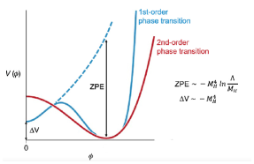
Figure 1: An intuitive picture which illustrates the crucial role of the ZPE in a first-order scenario of SSB. Differently from the standard second-order picture, these have to compensate for a tree-level potential with no non-trivial minimum.

At first sight, the nature of the phase transition may seem irrelevant, because nothing prevents the potential from having locally the same shape as in a second-order picture. To get more insight, let us look at Fig. 1. This intuitively illustrates that, if $V^{\prime\prime}_{\rm eff}(\phi=0)>0$, the ZPE is expected to be much larger than in a second-order picture. In the latter case, SSB is in fact driven by the negative mass-squared at $\phi=0$, whereas now the ZPE has to overwhelm a tree-level potential that otherwise would have no non-trivial minimum. Therefore, the ZPE mass scale $M_{H}$ and the mass scale $m_{h}$, defined by the quadratic shape of the effective potential at the minimum, could now be very different. Actually, a Renormalisation Group (RG) analysis of the effective potential indicates that these two masses scale differently with the ultraviolet cutoff $\Lambda$. Such an RG analysis is needed because, by “triviality”, at any finite scale $\mu$, the scalar self-coupling vanishes as $\lambda(\mu)\!\sim\ln^{-1}(\Lambda/\mu)$, where $\Lambda$ is the Landau pole fixing the cutoff scale. To minimise the cutoff dependence, one can thus consider the whole set of theories ($\Lambda$,$\lambda$), ($\Lambda^{\prime}$,$\lambda^{\prime}$), ($\Lambda^{\prime\prime}$,$\lambda^{\prime\prime}$), …, with larger and larger cutoff values, smaller and smaller low-energy couplings at $\mu$, but all sharing the same $\Lambda$-independent effective potential. There are then two RG-invariant quantities, namely the mass scale $M_{H}$ itself entering the minimum of the effective potential ${\cal E}\sim-M^{4}_{H}$ and a particular definition of the vacuum field to be used for the Fermi scale $v\sim 246$ GeV, which is always assumed to be cutoff independent. As such, they can be related by some finite proportionality constant, say $M_{H}=Kv$. Instead, for the smaller mass $m_{h}$ defining the quadratic shape of the potential, i.e., the inverse zero-momentum propagator $G^{-1}(p=0)$, one finds $m^{2}_{h}\sim M^{2}_{H}L^{-1}\sim v^{2}L^{-1}$ in terms of $L=\ln(\Lambda/M_{H})$, thus implying the traditional $\Phi^{4}$ relation $\lambda(v)=3m^{2}_{h}/v^{2}\sim L^{-1}$.

This mass structure was confirmed by explicit calculations of the propagator from the corresponding Gaussian Effective Action (GEA) [14], both for the one-component and $O(N)$-symmetric theory, with propagator

$$G^{-1}(p)=p^{2}+M^{2}_{H}A(p)\;.$$ (1)

Indeed, upon minimisation of the Gaussian potential, this gives [11] $G^{-1}_{h}(p)\sim p^{2}+m^{2}_{h}$ for $p\to 0$, where $A(p)\sim L^{-1}$, and $G^{-1}_{H}(p)\sim p^{2}+M^{2}_{H}$ at larger $p^{2}$, where $A(p)\sim 1$. The propagator structure in Eq. (1) was checked with lattice simulations which are considered a reliable non-perturbative approach. These simulations were also needed because the Gaussian-like approximations to the effective potential that we have considered predict the same qualitative scaling pattern but, resumming to all orders different classes of diagrams, yield different values of the numerical coefficient $c_{2}$ controlling the logarithmic slope, say $M^{2}_{H}\sim m^{2}_{h}L(c_{2})^{-1}$. Therefore, using numerical simulations [6], the best approximations to a free-field propagator could be found and so compute $m_{h}$ from the $p\to 0$ limit of $G(p)$, as well as $M_{H}$ from its behaviour at higher $p^{2}$. In this way, the expected logarithmic trend was checked and $c_{2}$ extracted. Referring to Ref. [6, 11], here we just summarise the final result. The value $(c_{2})^{-1/2}=0.67\,(3)$ from the lattice was replaced in the relation $M^{2}_{H}\sim m^{2}_{h}L(c_{2})^{-1}$, so that by combining with $m^{2}_{h}=\lambda(v)v^{2}/3$ and the leading-order trend $\lambda(v)\sim(16\pi^{2}/3)L^{-1}$ of $\Phi^{4}$, the finite proportionality relation $M_{H}=Kv$ was obtained, with $K=(4\pi/3)(c_{2})^{-1/2}$ or

$$(M_{H})^{\rm Theor}=Kv=690\,(30)\;{\rm GeV}\;.$$ (2)

3. Basic phenomenological aspects

The possible existence of a second, much larger mass $M_{H}\sim 690$ GeV associated with the ZPE implies that the known gauge and fermion fields would play a minor role for vacuum stability. In fact, by subtracting quadratic divergences or using dimensional regularisation, the logarithmically divergent terms in the ZPE due to the various fields are proportional to the fourth power of the mass, so in units of the pure scalar term one finds $(6M^{4}_{w}+3M^{4}_{Z})/M^{4}_{H}\lesssim 0.002$ and $12m^{4}_{t}/M^{4}_{H}\lesssim 0.05$. Besides, the two couplings $\lambda^{\rm(p)}(\mu)$ and $\lambda(\mu)$ coincide for $\mu=v$, so that their different evolution at large $\mu$ remains unobservable. Confirming this alternative mechanism of SSB then requires the observation of the second resonance and checking its phenomenology.

In this respect, the hypothetical $H$ is not like a standard Higgs boson of 700 GeV, as it would couple to longitudinal $W$s with the same typical strength as the low-mass state at 125 GeV [7, 11]. This can be explicitly shown by the Equivalence Theorem, when understood as a non-perturbative statement, valid to lowest non-trivial order in $g^{2}_{\rm gauge}$ but also to all orders in the scalar self-couplings [17]. This way, in longitudinal $WW$ scattering the contact coupling $\lambda_{0}=3M^{2}_{H}/v^{2}$, generated by the incomplete cancellation of graphs at tree level, is transformed into $\lambda(v)=3m^{2}_{h}/v^{2}=(m^{2}_{h}/M^{2}_{H})\lambda_{0}$ after resumming graphs to all orders. The equivalent argument is that it is $m_{h}=125$ GeV, and not $M_{H}\sim 700$ GeV which fixes the quadratic shape of the potential and the interaction with the Goldstone bosons.

Thus, the large conventional widths $\Gamma(H\to ZZ+WW)\sim G_{F}M^{3}_{H}$ would be suppressed by the small ratio $(m_{h}/M_{H})^{2}\sim 0.032$, leading to the estimates $\Gamma(H\to ZZ)\sim\frac{M_{H}}{700~{\rm GeV}}\,\times\,$(1.60 GeV) and $\Gamma(H\to WW)\sim\frac{M_{H}}{700~{\rm GeV}}\,\times\,$(3.27 GeV), besides the new contribution $\Gamma(H\to hh)\sim\frac{M_{H}}{700~{\rm GeV}}\,\times\,$(1.52 GeV). As such, the heavy $H$ should be a relatively narrow resonance of total width $\Gamma(H\to{\rm all})=25\div 35$ GeV, decaying predominantly to $t\bar{t}$ quark pairs, with a branching ratio of about 70$\div$80 $\%$. Note the very close branching ratios $B(H\to hh)\sim 0.95~B(H\to ZZ)$. Finally, due to its small coupling to longitudinal $W$s, $H$ production through vector-boson fusion (VBF) would be negligible as compared to gluon-gluon fusion (ggF), which has a typical cross section $\sigma^{\rm ggF}(pp\to H)\sim 1100\,(170)$ fb [18, 19], depending on QCD and $H$-mass uncertainties.

4. In touch with the experiments: ATLAS 4-lepton and $\gamma\gamma$ data

To get in touch with experiments, let us start from the four-lepton channel. In a first approximation, resonant four-lepton production at the $H$ peak could be estimated through the chain

$$\sigma_{R}\;\equiv\;\sigma_{R}(pp\to H\to 4l)\;\sim\;\sigma(pp\to H)\times B(H\to ZZ)\times 4B^{2}(Z\to l^{+}l^{-})\;,$$ (3)

with $4B^{2}(Z\to l^{+}l^{-})\sim 0.0045$. Thus, by substituting $\Gamma(H\to ZZ)\sim\frac{M_{H}}{700~{\rm GeV}}\,\times\,$(1.6 GeV), $\Gamma(H\to{\rm all})=25\div 35$ GeV, and $\sigma(pp\to H)\sim\sigma^{\rm ggF}(pp\to H)\sim 1100\,(170)$ fb, we would predict $\sigma_{R}\sim 0.26\,(7)$ fb.

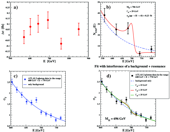
Figure 2: Panel a) shows the cross-section difference $\Delta\sigma$ between the experimental data and the expected background, as measured by ATLAS in the four-lepton channel [20]. The numerical values and energy bins can be found in Refs. [10, 11]. Panel b) shows the number of ATLAS ggF-low four-lepton events [21], grouped into bins of 60 GeV from 530 to 830 GeV. The blue dashed curve is the background while the red solid curve is the fit with Eq. (4). The numerical values and energy bins can be found in Refs. [10, 11]. Panel c) shows the invariant-mass distribution of the inclusive $\gamma\gamma$ events (converted to cross sections in fb), observed by ATLAS [22] in the range $\mu(\gamma\gamma)=E=600\div 770$ GeV and fitted with background only. The numerical values and energy bins can be found in Refs. [10, 11]. Finally, panel d) shows the fit to the data with Eq. (4), $M_{H}=696$ GeV, and three values of $\Gamma_{H}$.

In the previous analysis of Refs. [10, 11], a comparison was made to the data in Fig. 2. Its panel a) reports the cross-section difference $\Delta\sigma$ between the experimental data and the expected background, as measured by ATLAS in the four-lepton channel [20]. There is an excess-defect pattern that may indicate the characteristic change of sign of the interference past a Breit-Wigner peak. The numerical $\Delta\sigma$ and the size of the bins are given in Refs. [10, 11]. Here, for convenience of the reader, we just report the $\Delta\sigma$ for the four central bins from 585 to 800 GeV, whose individual values in fb are $0.085\pm 0.075$, $0.102\pm 0.078$, $0.136\pm 0.075$, and $-0.080\pm 0.050$, respectively. To describe these data, we have adopted the model of a resonance that interferes with a given background $\sigma_{b}(E)$, giving rise to a total cross section ($s=E^{2}$ and $\Gamma_{H}=\Gamma(H\to{\rm all})$)

$$\sigma_{T}(E)\;=\;\sigma_{b}(E)+\sigma_{R}\cdot R(E)+\sigma_{\rm int}(E)\;,$$ (4)

where

$$\sigma_{\rm int}(E)\;=\;2\sqrt{\sigma_{b}(E)\sigma_{R}}\,\frac{(M^{2}_{H}-s)}{\Gamma_{H}M_{H}}\,R(E)$$ (5)

and

$$R(E)\;=\;\frac{(\Gamma_{H}M_{H})^{2}}{(s-M^{2}_{H})^{2}+(\Gamma_{H}M_{H})^{2}}\;.$$ (6)

Some refinement is needed if one assumes the resonance to be produced through a specific parton process, e.g. through ggF as in our case. To implement this refinement and denoting as $\sigma^{\rm gg}_{b}$ the specific four-lepton background cross section from the ggF mechanism given in Ref. [20], the “non-ggF” background was preliminarily subtracted in Ref. [10, 11] by defining a modified experimental cross section

$$\hat{\sigma}_{\rm EXP}\;=\;\sigma_{\rm EXP}-(\sigma_{b}-\sigma^{\rm gg}_{b})$$ (7)

and then replacing everywhere $\sigma_{b}\to\sigma^{\rm gg}_{b}$ in the theoretical Eq. (4). The thus fitted values were $M_{H}=677^{+30}_{-14}$ GeV, $\Gamma_{H}=21^{+28}_{-16}$ GeV, and $\sigma_{R}=0.40^{+0.62}_{-0.34}$ fb. As an additional check, we also considered [9, 10, 11] the other data in panel b) of Fig. 2. This shows the statistically dominant ggF-low sample of ATLAS four-lepton events [21], grouped into bins of 60 GeV from 530 to 830 GeV. Fitting this other set of data gave similar results, viz. $M_{H}=706\,(25)$ GeV, $\Gamma_{H}=29\pm 20$ GeV, and $\sigma_{R}=0.23^{+0.28}_{-0.17}$ fb. However, this tentative agreement reflects the rather large error bars of the data. In fact, these events include a sizeable contribution from $q\bar{q}\to ZZ\to 4l$ processes that, strictly speaking, should not interfere with a resonance solely produced through the ggF mechanism. In any case, our expected mass $(M_{H})^{\rm Theor}=690\,(30)$ GeV and width $\Gamma_{H}=25\div 35$ GeV were well consistent with both types of fit.

Looking for other indications, the invariant-mass distribution of the inclusive $\gamma\gamma$ events observed by ATLAS [22] in the range $\mu(\gamma\gamma)=E=600\div 770$ GeV was also considered [9, 10, 11]. By parametrising the background with a power-law form $\sigma_{b}(E)\sim A\cdot({\rm 685~GeV}/E)^{\nu}$ one gets a good description of all data points, except for the sizeable excess at 684 GeV, which was estimated by ATLAS to have a local significance of more than $3\sigma$ (see panel c) of Fig. 2). This isolated discrepancy shows how a new resonance might remain hidden behind the large background nearly everywhere. For this reason, by fitting to Eq. (4), with the exception of the mass $M_{H}=$ 696 (12) GeV, the total decay width was determined very poorly, namely $\Gamma_{H}=15^{+18}_{-12}$ GeV. In panel d) of Fig. 2 we report three fits for $M_{H}=696$ GeV and $\Gamma_{H}=$ 15, 25, and 35 GeV, respectively.

Before concluding this section, two considerations are in order. First, with a definite prediction $(M_{H})^{\rm Theor}=690\,(30)$ GeV, one should look for deviations from the background nearby, say in the mass region 600$\div 800$ GeV, so that local deviations should not be downgraded by the so-called “look elsewhere” effect. Secondly, the local statistical significance of deviations from the background should take into account the phenomenology of a resonance that can produce both excesses and defects of events. For this reason, the statistical significance of the deviations from background seen in panel a) of Fig. 2 is actually $3\sigma$, like for the $\gamma\gamma$ data in panel c).

5. The CMS 4-lepton events

Table 1: We specify in the first three columns: the four-lepton invariant mass $m(4l)=E$, the expected CMS background events, and the experimental $S/B$ ratio reported in Fig. 7, upper left panel left, of Ref. [23], respectively. We then present the theoretical value of Eq. (9) for the optimal set of parameters obtained in the fit, viz. $M_{H}=692$ GeV, $\Gamma_{H}=10$ GeV, $N_{R}=0.55$, and the chi-squared of the fit. The numerical values of background events and experimental $S/B$ ratio, not reported in Ref. [23], were directly extracted from the figures. The accuracy is about 3$\div 4$%.

$\rm E$[GeV]	$N_{b}(E)$	[S/B]EXP	[S/B]Theory	$\chi^{2}$
645	1.46 (6)	1.10 (42)	1.14	0.01
660	1.33 (5)	1.20 (45)	1.21	0.00
675	1.20 (5)	1.56 (58)	1.41	0.07
690	1.09 (4)	1.93 (67)	1.88	0.01
705	0.99 (4)	0.54 (38)	0.58	0.01
720	0.90 (4)	1.19 (61)	0.76	0.50
735	0.82 (3)	0.98 (57)	0.83	0.07

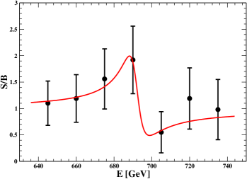
Figure 3: The fit with Eq. (9) to the data in Table 1 for $M_{H}=692$ GeV, $\Gamma_{H}=10$ GeV, and $N_{R}=0.55$. Note the close similarity with panels a) and b) of Fig. 2.

We will now compare with the recent, still preliminary CMS data for the four-lepton channel in Ref. [23]. To this end, we will first transform from Eq. (4) to the number of events $N$, for a given luminosity and acceptance, thus finding a total number

$$N_{\rm T}\;=\;N_{b}(E)+2\sqrt{N_{b}(E)N_{R}}\,\frac{(M^{2}_{H}-s)}{\Gamma_{H}M_{H}}\,R(E)+N_{R}R(E)$$ (8)

and a theoretical $S/B$ ratio

$$[S/B]^{\rm Theory}\;=\;1+2\sqrt{\frac{N_{R}}{N_{b}(E)}}\,\frac{(M^{2}_{H}-s)}{\Gamma_{H}M_{H}}\,R(E)+\frac{N_{R}}{N_{b}(E)}\,R(E)\;.$$ (9)

The CMS data for expected background events $N_{b}(E)$ and experimental $S/B$ ratio are given in Table 1. The combined deviation from unity of the three points at 675, 690, and 705 GeV is $2\sigma$. A fit to these data with Eq. (9) yields $M_{H}=692^{+17}_{-12}$ GeV, $\Gamma_{H}=10^{+26}_{-8}$ GeV, and $N_{R}=0.55^{+5.0}_{-0.45}$. The predictions of Eq. (9) for the optimal parameters are also presented in Table 1 and a graphical comparison is shown in Fig. 3.

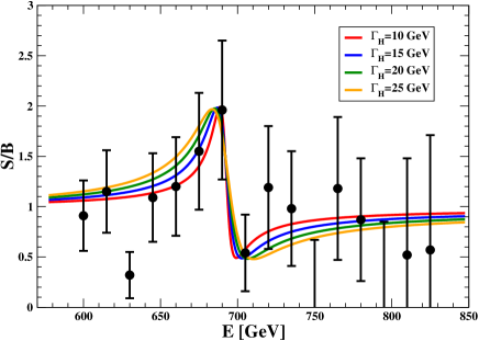
Figure 4: Comparing the CMS $S/B$ ratios to Eq. (9), for $M_{H}=692$ GeV, $N_{R}=0.55$, and four different widths.

To have a more complete idea of the overall agreement with the CMS data, we also enlarge the energy range from 600 to 800 GeV. The data for the $S/B$ ratio are then presented in Fig. 4, together with various curves for the same pair $M_{H}=692$ GeV, $N_{R}=0.55$ and different values of $\Gamma_{H}$. The more refined treatment of subtracting preliminarily the non-ggF background and comparing with the modified Eq. (7) is not possible here, in view of the very large error bars of the data.

6. CMS-TOTEM $\gamma\gamma$ events produced in $pp$ diffractive scattering

The CMS and TOTEM Collaborations have also been searching for high-mass photon pairs produced in $pp$ double-diffractive scattering, i.e., when both final protons are tagged and have large $x_{F}$. For our purpose, the relevant information is contained in Fig. 5 taken from Ref. [24]. In the range of invariant mass $650\,(40)$ GeV, and for a statistics of 102.7 fb^-1 the observed number of $\gamma\gamma$ events was $N_{\rm exp}\sim 76\,(9)$, to be compared with an estimated background $N_{\rm bkg}\sim 40\,(9)$. In the most conservative case, viz. $N_{\rm bkg}=49$, this represents a local $3\sigma$ effect and is the only statistically significant excess in the plot.

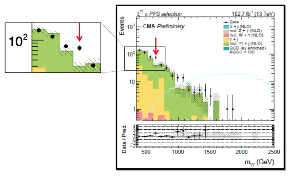
Figure 5: The number of $\gamma\gamma$ pairs produced in $pp$ diffractive scattering as reported in Ref. [24]. In the range $650\,(40)$ GeV, the observed number is $N_{\rm exp}\sim 76\,(9)$, to be compared to an estimated background $N_{\rm bkg}\sim 40\,(9)$.

7. The ATLAS $t\bar{t}$ events

The ATLAS Collaboration also searched for scalar resonances decaying to top-quark pairs [25]. There are small excesses at $675\,(75)$ GeV in the invariant mass of the $llbb$ system, which are more evident when the tracks of the final leptons are at large angles. The excess is minuscule, because the expected signal for a 700 GeV Higgs is about 1 pb, to be compared with a background cross section of $107.0\,(7.6)$ pb (see the CMS measurement [26] of top-quark pairs for invariant mass 620 $\div$ 820 GeV).

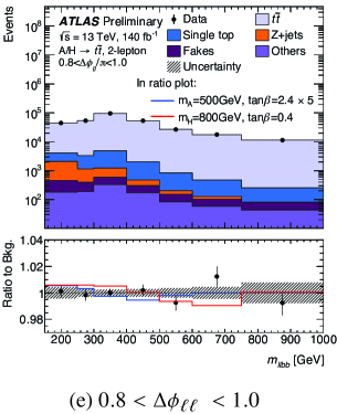
Figure 6: The slight excess of $t\bar{t}$ pairs observed by ATLAS for an invariant mass of the $llbb$ system around 675 GeV.

8. A closer look at the ATLAS $b\bar{b}+\gamma\gamma$ data

Table 2: For the bins $550\,(25)\div 800\,(25)$ GeV in Fig. 7, we report the experimental 95% upper limits $\sigma^{\rm exp}(j)$ for the cross section $\sigma(pp\to X\to hh)$ (black dots). The index $j=1\ldots 6$ indicates the bins $550\,(25),600\,(25),\ldots,800\,(25)$ GeV, respectively. Error bars in the experimental entries only take into account the $\sqrt{N}$ statistical uncertainty of the final $b\bar{b}+\gamma\gamma$ events. In the third column, we give the expected background values with $\pm 1\sigma$ and $\pm 2\sigma$ uncertainties (see the HEPData file of Ref. [27]).

j	$\sigma^{\rm exp}$(j) [fb]	$\sigma^{\rm bkg}$(j) [fb]
1	87.5 (15.6)	$95.1^{{+50.4}^{+137.3}}_{{-26.6}_{-44.1}}$
2	73.6 (14.3)	$81.1^{{+43.3}^{+119.0}}_{{-22.7}_{-37.6}}$
3	149.3 (20.3)	$84.4^{{+44.4}^{+120.1}}_{{-23.6}_{-39.1}}$
4	49.4 (12.0)	$76.5^{{+40.0}^{+109.6}}_{{-21.4}_{-35.4}}$
5	44.5 (12.0)	$71.7^{{+37.6}^{+103.3}}_{{-20.0}_{-33.2}}$
6	71.0 (14.0)	$65.8^{{+35.1}^{+96.5}}_{{-18.4}_{-30.5}}$

The ATLAS Collaboration has searched for a new resonance $X$ decaying, through a pair of $h=h(125)$ scalars, into the $b\bar{b}+\gamma\gamma$ final state [27]. Their results in Fig. 7 are given in terms of 95$\%$ upper limits for the cross section $\sigma(pp\to X\to hh)$, as a function of the invariant mass of the $b\bar{b}+\gamma\gamma$ system. The measured values, say $\sigma^{\rm exp}(j)$ in each bin $j$ (the black dots), are then compared with the expected limits, say $\sigma^{\rm bkg}$(j), along the black dashed line, by also allowing for $\pm 1\sigma$ and $\pm 2\sigma$ uncertainties in the theoretical predictions (see Table 2).

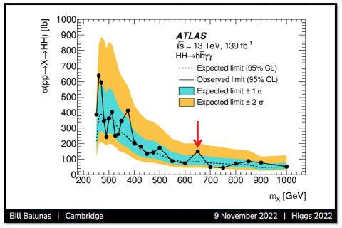
Figure 7: Expected and observed 95$\%$ upper limit for the cross section $\sigma(pp\to X\to h(125)h(125))$ obtained by ATLAS [27] from the final state $(b\bar{b}+\gamma\gamma)$. The figure is taken from the talk given by Bill Balunas at “Higgs 2022” and is the same as Fig. 15 in Ref. [27].

To compare with a resonance around 690 GeV, we will restrict ourselves to the mass range $550\div 800$ GeV. At first sight, this indicates a modest excess at $650\,(25)$ GeV, followed by two slight defects at 700 and 750 GeV. Such an excess-defect pattern could indicate the interference with the background around a Breit-Wigner peak and, in this interpretation, the mass would lie between 650 and 700 GeV, say $M_{H}\sim 675\,(25)$ GeV, where the interference changes sign. Now, the process $pp\to hh\to b\bar{b}+\gamma\gamma$ has also background contributions that should give no interference with a resonance solely produced by the ggF mechanism. Since differently from the four-lepton channel, the pure ggF contribution to the background $\sigma^{\rm gg}_{b}$ is not given explicitly here, one cannot adopt the most accurate procedure of first subtracting the non-ggF background and compare with Eq. (7). Besides, the ATLAS entries in Table 2 express upper bounds, so that, strictly speaking, one cannot fit with Eq. (4) to extract $M_{H}$ and $\Gamma_{H}$. Nonetheless, one can try to understand the order of magnitude of the main effect: the very large difference between the two entries at 650 and 700 GeV. To this end, let us assume a mass value $M_{H}\sim 675$ GeV. With the numerical values in Sec. 3, we then expect a peak cross section $\sigma_{R}=\sigma(pp\to H)B(H\to hh)\sim 55\,(10)$ fb, whose uncertainty comes mainly from the ggF production cross section, because both the partial and total decay widths scale linearly with mass. By also assuming $\Gamma_{H}\sim 25$ GeV and the same central values for the background as in the third column of Table 2, from Eq. (4) we would then expect the pair $\sigma_{T}(650)\sim 150$ fb and $\sigma_{T}(700)\sim 37$ fb, which lie very close to the experimental values

However, this is only a first level of comparison with these data. Our point is that the modest statistical consideration, given so far to the ATLAS $b\bar{b}+\gamma\gamma$ data, was substantially influenced by the large uncertainty in the expected limits, as given by the wide blue and yellow bands around the central dashed line in Fig. 7. The uncertainty in each absolute value of the cross sections is indeed large, but this is not the right perspective. In fact, in our mass region and to a very good approximation, the whole effect of these uncertainties is simply to shift the line of the central values up and down. For instance, at 650 GeV the experimental value $149.3\,(20.3)$ fb is well within the $+2\sigma$ limit for the background $84.4+120.1=204.5$ fb. But if we now evaluate the difference between the experimental values at 650 and 600 GeV, which is $149.3\,(20.3)-73.6\,(14.3)=75.7\,(24.8)$ fb, this is much larger than the corresponding background differences, either along the black central line $84.4-81.1=3.3$ fb or along the $1\sigma$ and $2\sigma$ contours, being $128.8-124.4=4.4$ fb and $204.5-200.1=4.4$ fb, respectively. That would now give a discrepancy of about $2.9\sigma$.

Therefore, we have done the exercise of comparing the experimental differences in consecutive energy bins

$$\Delta^{\rm exp}(j+1,j)\;=\;\sigma^{\rm exp}(j+1)-\sigma^{\rm exp}(j)$$ (10)

with the corresponding expected values $\Delta^{\rm bkg}(j+1,j)=\sigma^{\rm bkg}(j+1)-\sigma^{\rm bkg}(j)$, which remain nearly constant when evaluated on the black line or along the corresponding boundaries of the blue and yellow bands; see Table 3.

Table 3: The experimental difference $\Delta^{\rm exp}(j+1,j)=\sigma^{\rm exp}(j+1)-\sigma^{\rm exp}(j)$ in fb, as computed from the values in Table 2. We also report the expected backround values $\Delta^{\rm bkg}(j+1,j)$. The latter are computed on the black dashed line and along the corresponding boundaries of the blue and yellow bands.

$\Delta^{\rm exp}(2,1)=-13.9\pm 21.1$	$\Delta^{\rm bkg}(2,1)=-19.9\pm 12.4$
${\Delta^{{\rm{exp}}}(3,2)}={+75.7\pm 24.8}$	${\Delta^{{\rm{bkg}}}(3,2)}={+3.1\pm 1.4}$
${\Delta^{{\rm{exp}}}(4,3)}={-99.9\pm 23.6}$	${\Delta^{{\rm{bkg}}}(4,3)}={-11.4\pm 7.2}$
$\Delta^{\rm exp}(5,4)=-4.9\pm 17.0$	$\Delta^{\rm bkg}(5,4)=-6.8\pm 4.2$
${\Delta^{{\rm{exp}}}(6,5)}={+26.5\pm 18.4}$	${\Delta^{{\rm{bkg}}}(6,5)}={-7.9\pm 4.7}$

Looking at Table 3, the results are seen to indicate that the large difference between the fourth and third experimental entries, viz. $-99.9\pm 23.6$ fb, cannot be explained by theoretical uncertainties, which would rather predict a difference in the range $-11.4\pm 7.2$ fb. Here, the discrepancy is about $3.4\sigma$ and goes in the opposite direction. By also including the discrepancy of $1.6\sigma$ between the fifth pair of entries, the combined deviations reach the level of about $3.8\sigma$.

Other interesting observables are the measured ratios

$$R^{\rm exp}(j,j+1)\;=\;\frac{\sigma^{\rm exp}(j)}{\sigma^{\rm exp}(j+1)}\;,$$ (11)

because systematic effects, as many of those reported in Table VIII of Ref. [27] and which modify the overall normalisation of the data, would cancel out. We have thus compared in Table 4 with the corresponding background quantities $R^{\rm bkg}(j,j+1)=\sigma^{\rm bkg}(j)/\sigma^{\rm bkg}(j+1)$. From the $4\sigma$ difference in the second row and the $2.2\sigma$ difference in the fifth row, this would now give a combined value of about $4.5\sigma$. However, there is some ambiguity here, because by replacing $j\to j+1$ and $j+1\to j$ in Table 4 error bars now become asymmetric and the individual deviations are not the same. This ambiguity is not present in the $\Delta$s, because with the replacements $j\to j+1$ and $j+1\to j$ there is only a change of sign and the statistical significance of any deviation remains the same. For this reason, we will limit ourselves to consider the deviations observed in the $\Delta$s.

Table 4: The experimental ratios $R^{\rm exp}(j,j+1)=\sigma^{\rm exp}(j)/\sigma^{\rm exp}(j+1)$, as computed from the values in Table 2. We also report the expected background values of $R^{\rm bkg}(j,j+1)$. The latter are computed at the points on the black dashed line for each pair of bins $j$ and $j+1$, as well as along the corresponding boundaries of the blue and yellow bands.

$R^{\rm exp}(1,2)=1.19(31)$	$R^{\rm bkg}(1,2)=1.18(1)$
${R^{{\rm{exp}}}(2,3)}={0.49(12)}$	${R^{{\rm{bkg}}}(2,3)}={0.97(1)}$
${R^{{\rm{exp}}}(3,4)}={3.02(84)}$	${R^{{\rm{bkg}}}(3,4)}={1.10(1)}$
$R^{\rm exp}(4,5)=1.11(38)$	$R^{\rm bkg}(4,5)=1.07(1)$
${R^{{\rm{exp}}}(5,6)}={0.63(21)}$	${R^{{\rm{bkg}}}(5,6)}={1.09(1)}$

Before concluding, we observe an interesting correlation. From the two ATLAS bins at 700 and 750 GeV one finds a ratio $R^{\rm exp}(4,5)\sim 1.11$ that nearly coincides with the corresponding background value $R^{\rm bkg}(4,5)\sim 1.07$. This is because the two values in Table 2, viz. $\sigma^{\rm exp}(4)\sim 49.4$ fb and $\sigma^{\rm exp}(5)\sim 44.5$ fb, while considerably smaller than the corresponding average background values $\langle\sigma^{\rm bkg}(4)\rangle=76.5$ fb and $\langle\sigma^{\rm bkg}(5)\rangle=71.7$ fb, give the same average $\langle S/B\rangle\sim$ 0.63. A possible explanation can be obtained by looking at the CMS data for the $S/B$ in Fig. 4. This shows that the bins at 750 and 795 GeV are empty, with their error bars representing the CMS estimates for the upper limits which one could expect with more statistics, about 0.66 and 0.86, respectively. Note that the first upper bound at 750 GeV is only slightly higher than the lower bound, about 0.58, obtained from the bin at 720 GeV. In view of the large error bars of the remaining points, this means that values with $S/B$ considerably smaller than unity have a large probability content. The theoretical curves, especially those of green and yellow colour for widths 20$\div$25 GeV, can thus provide a clue with their prediction of a slow increase in $S/B$ from about 0.5 at 705 GeV up to about 0.8 at 800 GeV, with an average value $S/B\sim 0.65\,(15)$. Still focusing on the four-lepton channel, let us return to panel a) of Fig. 2 and to the difference $\Delta\sigma=-0.080\,(50)$ fb between the average cross section $\langle\sigma^{\rm exp}(4l)\rangle=0.126\,(47)$ fb measured by ATLAS in the range $720\div 800$ GeV and the corresponding expected background $\langle\sigma^{\rm bkg}(4l)\rangle=0.206\,(18)$ fb; see Table 4 of Ref. [11]. From the ratio of these two cross sections, we thus obtain the average ratio $S/B=0.61\,(23)$ measured by ATLAS and, in view of its consistency with the previous value $0.65\,(15)$, an average combined $\langle S/B\rangle^{\rm 4l}=0.64\,(13)$ from the four-lepton channel past the resonance peak. Since $M_{H}$ and $\Gamma_{H}$ are the same for both $pp\to H\to ZZ$ and $pp\to H\to hh$, and the two branching ratios $B(H\to hh)$ and $B(H\to ZZ)$ are very close, we can use this combined value to describe the analogous reduction of events observed in the $b\bar{b}+\gamma\gamma$ final state. The predicted averages

$$\langle\sigma(4)\rangle\sim\langle S/B\rangle^{\rm 4l}\langle\sigma^{\rm bkg}(4)\rangle\;=\;49.0\,(9.9)\>{\rm fb}\;\;\;{\rm and}\;\;\;\langle\sigma(5)\rangle\sim\langle S/B\rangle^{\rm 4l}\langle\sigma^{\rm bkg}(5)\rangle\;=\;45.9\,(9.3)\>{\rm fb}$$ (12)

are then in very good agreement with the experimental values in Table 2, confirming at the same time the accuracy of the average background estimates. The existence of this correlation, between four-lepton and $b\bar{b}+\gamma\gamma$ final states, could hardly be explained without the second resonance.

Summarising: in the region of invariant mass that is crucial for the predicted second resonance $H$ of the Higgs field, the ATLAS determinations of the cross section $\sigma^{\rm exp}(pp\to X\to hh)$ from the $b\bar{b}+\gamma\gamma$ channel [27] exhibit the same characteristic excess-defect pattern observed by ATLAS and CMS in the four-lepton channel. The natural interpretation is in terms of a resonance with mass $M_{H}\sim 675\,(25)$ GeV. To estimate precisely the statistical significance of the measurements, we have considered the differences of the $\sigma^{\rm exp}(j)$ in consecutive bins and compared with the corresponding combinations of the $\sigma^{\rm bkg}(j)$, where all theoretical uncertainties nearly vanish. The combined statistical significance of the observed deviations could then be estimated at the level of about $3.8\sigma$. Of course, this is the statistical significance with our experimental error bars (always larger than the size $\pm 12$ fb of the black dots in Fig. 7), which only take into account the statistical uncertainty in the determinations of the final $b\bar{b}+\gamma\gamma$ events. On the other hand, while it is true that no other source of uncertainty is included, systematic effects, as many of those reported in Table VIII of Ref. [27] and affecting the overall normalisation of the data, would cancel out in the ratios that also exhibit large deviations.

9. Summary and conclusions

In the present paper, we have first briefly summarised an alternative picture of SSB, which predicts a relatively narrow second resonance of the Higgs field, with mass $(M_{H})^{\rm Theor}=690\,(30)$ GeV. We then started to compare with the LHC data. Here, one should take into account three aspects that characterise this particular research. First, with a definite prediction $(M_{H})^{\rm Theor}=690\,(30)$ GeV, one should look for deviations from the background nearby, say in the mass region 600$\div 800$ GeV, so that local deviations cannot be downgraded by the so called “look elsewhere” effect.

Secondly, given the present integrated luminosity collected at the LHC, the second resonance is too heavy to be seen unambiguously by both experimental collaborations and in all possible channels. In retrospect, one should remember the discovery of the 125 GeV resonance in 2012, which was initially seen by ATLAS and CMS predominantly in the $h\to\gamma\gamma$, $h\to ZZ\to$ four-charged-leptons channels, and confirmed in the $h\to WW$ channel (with lower significance). However, it was not seen in the dominant $b\bar{b}$ channel and in the important $\tau^{+}\tau^{-}$ channel, which were expected to be quite sensitive. The channels crucial for the discovery, with the statistics available at that time, were those in which the final states were fully reconstructed and contained photons or $e^{+}e^{-},\,\mu^{+}\mu^{-}$ pairs, providing the best invariant-mass resolution. Presumably, this continues to be the case even in the search for a high-mass neutral resonance, so that the absence of signals in potentially sensitive channels, but with lower invariant-mass resolution, should not be surprising.

Thirdly, the statistical significance of deviations from the background should be evaluated by taking into account the phenomenology of a resonance that can produce both excesses and defects of events.

With these premises, our review of LHC data is summarised next:

• The ATLAS data for the four-lepton channel, both for the cross section and the statistically dominant class of ggF-low events, show deviations from the background with a definite excess-defect sequence which are typical for a resonance; see panels a) and b) of Fig. 2. By subtracting from the cross-section data the non-ggF background, a fit with Eq. (4) gives a mass $M_{H}=677^{+30}_{-14}$ GeV. The combined statistical significance of the observed deviation is $3\sigma$.

• The ATLAS inclusive $\gamma\gamma$ events indicate a $3\sigma$ excess at $684$ GeV; see panel c) of Fig. 2. A fit to the data with Eq. (4) (see panel d) of Fig. 2) yields a resonance mass $M_{H}=696\,(12)$ GeV.

• For the $S/B$ in the CMS four-lepton channel (see Table 1), by considering the three values at 675, 690, and 705 GeV, one finds a combined deviation of $2\sigma$. The fitted mass (see Fig. 3) comes out at $M_{H}=692^{+17}_{-12}$ GeV.

• The CMS-TOTEM $\gamma\gamma$ events produced in $pp$ diffractive scattering indicate an excess of $3\sigma$ in the region of invariant mass $M_{H}=650\,(40)$ GeV (see Fig. 5).

• The ATLAS data for top-quark pair production, indicate small excesses at a mass of $675\,(75)$ GeV, which are more evident when the tracks of the final leptons are at large angles; see Fig. 6. The statistical significance is $1\sigma$.

• ATLAS measurements in the $b\bar{b}+\gamma\gamma$ channel [27] to constrain the cross section $\sigma^{\rm exp}(pp\to X\to hh)$ indicate the same excess-defect pattern observed in the four-lepton channel by both ATLAS (see panels a) and b) Fig. 2) and CMS (see Fig. 3). Since this is the characteristic signature of background-resonance interference, here the resonance mass would be $M_{H}\sim 675\,(25)$ GeV. We have also shown that the importance of these ATLAS measurements has been overlooked. In fact, one can construct particular combinations of the cross sections in consecutive bins where all theoretical uncertainties practically vanish. The combined statistical significance is thus large, at the level of about $3.8\sigma$, implying that the observed deviations cannot be simple statistical fluctuations. This is even more true as one can use the tendentially low $S/B$ ratio, past the resonance peak and observed by both ATLAS and CMS in the four-lepton channel, to explain the sizeable reduction of $b\bar{b}+\gamma\gamma$ events seen by ATLAS in the same region of invariant mass.

Since the above determinations are all well aligned within their respective uncertainties, we can combine the mass values and obtain $(M_{H})^{\rm comb}\sim 685\,(10)$ GeV, in very good agreement with our prediction $(M_{H})^{\rm Theor}=690\,(30)$ GeV. Due to the modest correlation of the above measurements, we could also attempt a rough estimate of the combined statistical evidence through the sum of the squares of the individual sigmas. The combined results, at the level of about $5.8\sigma$ from ATLAS and $3.6\sigma$ from CMS, definitely exclude an interpretation in terms of statistical fluctuations.

Thus, by increasing the statistics and refining the analysis, we expect the second resonance to also show up in other channels. But these other channels, where the second resonance has not yet been seen, cannot represent an argument to exclude its existence. As an example, let us consider the process $H\to WW\to 2l2\nu$. As explained, the second resonance is essentially produced via the ggF mechanism. Therefore, when comparing with the existing CMS measurements [28], the second resonance is in the class of models where the VBF production mode is irrelevant. This is the case $f_{\rm VBF}=0$ in Fig. 4 (top left) of Ref. [28]. From the numbers reported in our Sec. 3., namely a partial width $\Gamma(H\to WW)\sim 3.27$ GeV and a total width $\Gamma(H\to{\rm all})\sim 25\div 35$ GeV, we find a branching ratio $B(H\to WW)\sim 0.11\,(2)$. Thus, for a ggF production cross section of about 1 pb, we expect a resonant contribution $\sigma(pp\to H\to WW\to 2l2\nu)\sim 5\,(1)\times 10^{-3}$ pb, well consistent with the CMS 95% upper limit of $0.02\div 0.03$ pb around 700 GeV. On the other hand, we could also consider another CMS search for heavy resonances $X$, viz. through the chain $X\to hh\to b\bar{b}WW$. From Fig. 18 (upper panel) of Ref. [29], the $S/B$ ratio is seen to decrease from about 1.5 at 600 GeV down to about 0.5 at 750 GeV. Here, the latter 2$\sigma$ defect would be consistent with the previous average determination $\langle S/B\rangle=0.65\,(15)$, observed by both ATLAS and CMS in the four-lepton channel, as well as by ATLAS in the $b\bar{b}+\gamma\gamma$ final state, past the resonance peak. As such, it could be brought in support of our picture.

Analogous considerations could be applied to other samples of data where the weakness of the expected signal and/or the low statistics do not allow for stringent tests. Instead, a serious problem is that, nowadays, experiments are compared to substantial modifications of the Standard Model (such as explicit additional Higgs bosons, supersymmetric extensions, extra space-time dimensions, …). However, no attention is paid to the simplest idea, namely that the same SM Higgs field may exhibit a richer pattern of mass scales, like when SSB in $\Phi^{4}$ theory is described as a (weak) first-order phase transition. In view of the sizeable deviations we have pointed out, we hope that the experimental groups will now also consider this other possibility.

References

- [1] G. Aad et al. [ATLAS Collaboration], Phys. Lett. B 716, 1 (2012).
- [2] S. Chatrchyan et al. [CMS Collaboration], Phys. Lett. B 716, 30 (2012).
- [3] V. Branchina, E. Messina, Phys. Rev. Lett. 111, 241801 (2013).
- [4] E. Gabrielli, et al. Phys. Rev. D 89, 015017 (2014).
- [5] J. R. Espinosa, G. Giudice, A. Riotto, JCAP 05, 002 (2008).
- [6] M. Consoli, L. Cosmai, Int. J. Mod. Phys. A 35 (2020) 2050103, hep-ph/2006.15378.
- [7] M. Consoli, Acta Phys. Pol. B 52 (2021) 763; arXiv: 2106.06543 [hep-ph].
- [8] M. Consoli, L. Cosmai, Int. J. Mod. Phys. A 37 (2022) 2250091; arXiv:2111.08962v2 [hep-ph].
- [9] M. Consoli, L. Cosmai, F. Fabbri, Universe 9 (2023).
- [10] M. Consoli, G. Rupp, Lett. High Energy Phys., LHEP-515, 2024; arXiv:2404.03711 [hep-ph].
- [11] M. Consoli , G. Rupp, Eur. Phys. J. C (2024) , 84:951; arXiv:2308.01429v3 [hep-ph].
- [12] S. R. Coleman, E. J. Weinberg, Phys. Rev. D 7, 1888 (1973) 1888.
- [13] S. Akiyama, Y. Kuramashi, T. Yamashita, Y. Yoshimura, Phys. Rev. D 100, 054510 (2019).
- [14] A. Okopinska, Phys. Lett. B 375 (1996), 213.
- [15] C. B. Lang, NATO Sci. Ser. C 449, 133 (1994)
- [16] U. M. Heller, Nucl. Phys. B Proc. Suppl. 34, 101 (1994)
- [17] J. Bagger, C. Schmidt, Phys. Rev. D 41, 264 (1990).
-
[18]
“BSM Higgs production cross sections at TeV
(update in CERN Report4 2016)”
https://twiki.cern.ch/twiki/bin/view/LHCPhysics/
CERNYellowReportPageBSMAt13TeV -
[19]
“SM Higgs production cross sections at TeV
(update in CERN Report4 2016)”
https://twiki.cern.ch/twiki/bin/view/LHCPhysics/
CERNYellowReportPageAt13TeV - [20] G. Aad et al. [ATLAS Collaboration], JHEP 07, 005 (2021).
- [21] G. Aad et al. [ATLAS Collaboration], Eur. Phys. J. C 81, 332 (2021).
- [22] G. Aad et al. [ATLAS Collaboration], Phys. Lett. B 822, 136651 (2021).
- [23] The CMS Collaboration, “Search for heavy scalar resonances decaying to a pair of Z bosons in the 4-lepton final state at 13 TeV”, CMS PAS HIG-24-002, 20 July 2024.
- [24] CMS and TOTEM Collaborations, Phys. Rev. D 110 (2024) 012010; arXiv:2311.02725 [hep-ex].
- [25] ATLAS Collaboration, “Search for heavy neutral Higgs bosons decaying to a top quark pair in 140 fb-1 of proton–proton collision data at TeV, ATLAS-CONF-2024-001, March 16, 2024.
- [26] A. M. Sirunyan et al. [CMS Collaboration], JHEP 02, 149 (2019).
- [27] G. Aad et al. [ATLAS Collaboration], Phys. Rev. D 106, 052001 (2022).
- [28] CMS Collaboration, CMS PAS HIG-20-016, 2022/03/11.
- [29] CMS Collaboration, CMS PAS HIG-21-005, 2023/03/27.