Spectral representation of correlation functions for zeros of Gaussian power series with stationary coefficients

Tomoyuki SHIRAI Institute of Mathematics for Industry, Kyushu University, 744 Motooka, Nishi-ku, Fukuoka 819-0001, Japan shirai@imi.kyushu-u.ac.jp
(Date: 2025/2/5)
Abstract.

We analyze Gaussian analytic functions (GAFs) defined as power series with coefficients modeled by discrete stationary Gaussian processes, utilizing their spectral measures. We revisit some limit theorems for random analytic functions and examine some examples of GAFs through numerical computations. Furthermore, we provide an integral representation of the $n$-point correlation functions of the zero sets of GAFs in terms of the spectral measures of the underlying coefficient Gaussian processes.

2020 Mathematics Subject Classification:
30B20; 30C15; 60G15; 60G55

1. Introduction

Gaussian analytic functions (GAFs) have attracted significant interest and have been extensively studied by many researchers (cf. [17, 32, 33, 15] and references therein). One of the striking results in the study of GAFs is that the zeros of random power series $\sum_{n=0}^{\infty}\zeta_{n}z^{n}$ with i.i.d. complex Gaussian coefficients $\{\zeta_{n}\}_{n=0}^{\infty}$, whose covariance kernel is the Szegő kernel, form the determinantal point process (DPP) on the unit disk associated with the Bergman kernel $(1-z\bar{w})^{-2}$ [27] (see for details on DPPs (cf. [30, 35, 31, 15]). As a natural generalization of this model, various related models have been studied. The singular points of random matrix-valued Gaussian analytic functions are shown to form the DPPs associated with weighted Bergman kernel $(1-z\bar{w})^{-\alpha}$ [21]. The zeros of random power series $\sum_{n=0}^{\infty}\zeta^{\mathbb{R}}_{n}z^{n}$ with i.i.d. real Gaussian coefficients $\{\zeta^{\mathbb{R}}_{n}\}_{n=0}^{\infty}$, which is the limiting Kac random polynomial, form the Pfaffian point process on the unit disk [11, 22]. The Gaussian Laurant series whose covariance kernel is the weighted Szegő kernel on an annulus was studied in [18]. We are concerned with the zeros of Gaussian power series $\sum_{n=0}^{\infty}\xi_{n}z^{n}$ with coefficients being stationary, centered, complex Gaussian process $\{\xi_{n}\}_{n=0}^{\infty}$. In [24, 29], we discussed the expected number of zeros within a disk and the density of zeros in the radial direction, observing their asymptotic behavior as the radius approaches the circle of convergence. Our observations reveal that the spectral measure of the coefficient Gaussian process plays a crucial role in determining the asymptotic behavior of the number of zeros near the radius of convergence. From the viewpoint of the spectral measure, the zeros of Gaussian analytic functions in a strip in the complex plane, with translation-invariant distribution, are studied in [9, 10]. This line of study traces back to the work of Paley and Wiener [25]. In [2, 3, 1], the authors investigate random power series and their zeros from the perspective of spectral measures (or limiting empirical spectral measures in the case of deterministic coefficients), considering cases where the coefficients are not necessarily Gaussian processes but weakly stationary processes, and even in certain cases where the coefficients are deterministic.

In this paper, we also emphasize the spectral perspective to study the zeros of GAFs. The remainder of this paper is organized as follows. In Section 2, we review the Edelman-Kostlan formula for the $1$-point correlation function and give its spectral representation. We also recall some results of limit theorems for random analytic funcitons established in [28]. In Section 3, we explore examples of GAFs associated with three different spectral measures and present some numerical computations. In Section 4, we provide a spectral representation of the $n$-point correlation function for the zeros of a GAF whose covariance kernel is a stationary complex Gaussian process. As an example of this represetation result, we compute certain quantities related to the i.i.d. coefficients case to illustrate the Peres-Virág theorem.

2. Gaussian analytic functions and their spectral representation

2.1. Spectral representation of GAF and the intensity of its zeros

Let $\Xi=\{\xi_{k}\}_{k\in\mathbb{Z}}$ be a stationary, centered, complex Gaussian process with covariance

$$\gamma(k-l)=\mathbb{E}[\xi_{k}\overline{\xi_{l}}].$$

Throughout the paper, we assume that $\gamma(0)=1$, i.e., the distribution of each marginal $\xi_{k}$ is complex standard normal. We consider the Gaussian power series with dependent coefficients $\Xi=\{\xi_{k}\}_{k\in\mathbb{Z}}$ defined by

$$X_{\Xi}(z):=\sum_{k=0}^{\infty}\xi_{k}z^{k}$$

and its zeros. Since the radius of convergence of $X_{\Xi}(z)$ is equal to $1$ a.s. under $\gamma(0)=1$, the zeros of $X_{\Xi}(z)$ form a point process $\mathcal{Z}_{X_{\Xi}}:=\sum_{z\in\mathbb{D}:X_{\Xi}(z)=0}\delta_{z}$ on $\mathbb{D}:=\{z\in\mathbb{C}:|z|<1\}$. We denote the covariance kernel of the GAF $\mathbb{X}=\{X_{\Xi}(z)\}_{z\in\mathbb{D}}$ by $K(z,w)$. Then, we have the spectral representation of $K(z,w)$ [29] as

$$K(z,w)=\mathbb{E}[X_{\Xi}(z)\overline{X_{\Xi}(w)}]=\int_{\mathbb{T}}s(z,t)\overline{s(w,t)}F(dt),$$ (2.1)

where $\mathbb{T}=(-\pi,\pi]$, the kernel $s(z,t)$ is given by the Szegő kernel

$$s(z,t)=\frac{1}{1-ze^{-it}}\quad(z\in\mathbb{D},t\in\mathbb{T})$$ (2.2)

and $F(dt)$ is the spectral measure of the coefficient Gaussian process $\Xi$ [7], i.e., $F(dt)$ is a probability measure on $\mathbb{T}$ (since $\gamma(0)=1$) such that

$$\gamma(k)=\int_{\mathbb{T}}e^{-ikt}F(dt).$$

We denote the right-hand side of (2.1) by $K_{F}(z,w)$. Since $|s(z,t)|^{2}=(1-2r\cos(\theta-t)+r^{2})^{-1}$ for $z=re^{i\theta}$, the covariance kernel $K_{F}(z,z)$ for $z=re^{i\theta}$ can be expressed as

$$K_{F}(z,z)=\frac{1}{1-r^{2}}\int_{\mathbb{T}}P(r,\theta-t)F(dt),$$ (2.3)

where $P(r,\theta)$ is the Poisson kernel given by

$$P(r,\theta)=\frac{1-r^{2}}{1-2r\cos\theta+r^{2}}.$$ (2.4)

The first intensity (or $1$-point correlation function) of the zeros of a GAF can be computed from the covariance kernel $K(z,w)$ by the Edelman-Kostlan formula [8] as follows:

Theorem 2.1 (Edelman-Kostlan).

Let $X=(X(z))_{z\in D}$ be a GAF with convariance $K(z,w)=\mathbb{E}[X(z)\overline{X(w)}]$. Then, the first intensity of zeros of $X(z)$ is given by the formula

$$\rho_{1}(z)=\frac{1}{\pi}\partial_{z}\partial_{\bar{w}}\log K(z,w)\Big{|}_{w=z}.$$

When $K(z,w)$ is of the form (2.1), using the fact that $\partial_{z}s(z,t)=e^{-it}s(z,t)^{2}$ and the symmetrization of the variable $t$, we can see that

$$\rho_{1}(z)=\frac{1}{2\pi K(z,z)^{2}}\int_{\mathbb{T}^{2}}|e^{-it}-e^{-iu}|^{2}|s(z,t)s(z,u)|^{4}F(dt)F(du)\quad(z\in\mathbb{D}).$$ (2.5)

In Section 4, we will provide an integral representation of the $n$-point correlation function of the zeros.

2.2. Convergence of random analytic functions and their zero processes

Let $D\subset\mathbb{C}$ be a domain and $\mathcal{H}(D)$ be the space of complex analytic functions on $D$ equipped with the metric

$$\rho(f,g)=\sum_{j=1}^{\infty}\frac{1}{2^{j}}\frac{\|f-g\|_{K_{j}}}{1+\|f-g\|_{K_{j}}},$$

where $\|f\|_{K}$ is the supremum norm of $f$ on a compact set $K$ and $K_{1}\subset K_{2}\subset\dots\nearrow D$ is an exhaustion of $D$ by compact sets $K_{j}$. The metric space $(\mathcal{H}(D),\rho)$ turns out to be complete and separable. We denote the totality of probability measures on $\mathcal{H}(D)$ by $\mathcal{P}(\mathcal{H}(D))$. We call an $\mathcal{H}(D)$-valued random variable a random analytic function. We recall the following fact established in [28, Proposition 2.5 with Remark on page 341]).

Proposition 2.2.

Let $D\subset\mathbb{C}$ be a domain and $\{X_{n}\}_{n=1}^{\infty}$ be a sequence of random analytic functions on $D$. If $\sup_{n}\mathbb{E}[|X_{n}(z)|^{p}]$ is locally integrable on $D$ for some $p>0$, then $\{\mu_{X_{n}}\}_{n=1}^{\infty}$ is tight in $\mathcal{P}(\mathcal{H}(D))$. Moreover, if $\{X_{n}\}_{n=1}^{\infty}$ converges to $X$ in the sense of finite-dimensional distributions, then $\{\mu_{X_{n}}\}$ converges weakly to $\mu_{X}$ as $n\to\infty$, or equivalently, $\{X_{n}\}_{n=1}^{\infty}$ converges to $X$ in law.

We also recall the convergence of zero processes [28, Proposition 2.3].

Proposition 2.3.

A sequence of random analytic functions $\{X_{n}\}_{n=1}^{\infty}$ converges in law to $X$. Then, the zero process $\mathcal{Z}_{X_{n}}$ converges in law to $\mathcal{Z}_{X}$ provided that $X\not\equiv 0$ almost surely.

We apply these results to our current situation. Let $X_{F}=\{X_{F}(z)\}_{z\in\mathbb{D}}$ be the GAF corresponding to the covariance kernel

$$K_{F}(z,w)=\int_{\mathbb{T}}s(z,t)\overline{s(w,t)}F(dt).$$ (2.6)
Corollary 2.4.

Let $F_{n}(dt),n=1,2,\dots$ and $F(dt)$ be probability measures on $\mathbb{T}$ and suppose that $\{F_{n}(dt)\}_{n=1}^{\infty}$ converges weakly to $F(dt)$. Then, $X_{F_{n}}$ corresponding to $F_{n}$ converges in law to $X_{F}$ corresponding to $F$. Moreover, the zero process $\mathcal{Z}_{X_{F_{n}}}$ converges in law to that of $\mathcal{Z}_{X_{F}}$.

Proof.

The local integrability of $\sup_{n}\mathbb{E}[|X_{F_{n}}(z)|^{2}]$ follows from the fact that $\mathbb{E}[|X_{F_{n}}(z)|^{2}]=K_{F_{n}}(z,z)\leq(1-|z|)^{-2}$ for every $n$. Since $s(z,t)$ is bounded continuous in $t$ for every $z\in\mathbb{D}$, by the weak convergence of $\{F_{n}\}_{n=1}^{\infty}$ to $F$, $K_{F_{n}}(z,w)$ converges to $K_{F}(z,w)$ for every $z,w\in\mathbb{D}$. This implies that $X_{F_{n}}$ converges to $X_{F}$ in the sense of finite-dimensional distributions. Therefore, $X_{F}$ converges in law to $X$ by Proposition 2.2. The zero processes $\mathcal{Z}_{F_{n}},n=1,2,\dots$ converges in law to $\mathcal{Z}_{F}$ Proposition 2.3 since $X_{F}\not\equiv 0$ almost surely. ∎

3. Examples

Using Propositions 2.2, 2.3 and Corollary 2.4, we discuss three examples.

3.1. The case $F(dt)=dt/(2\pi)$

In this case, we easily see that $\gamma_{F}(k)=\delta_{k,0}$ and the kernel $K_{F}(z,w)$ is given by

$$K_{F}(z,w)=\int_{\mathbb{T}}s(z,t)\overline{s(w,t)}\frac{dt}{2\pi}=\frac{1}{1-z\bar{w}}\quad(z,w\in\mathbb{D}),$$

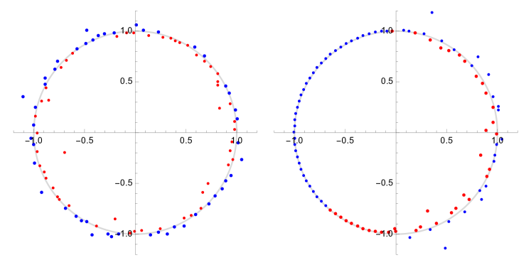
which is also called the Szegő kernel. The kernel $s(z,t)$ is the boundary value of $(1-z\bar{w})^{-1}$ at $w=e^{it}$. This spectral measure corresponds to the i.i.d. coefficients case. This GAF is sometimes called the hyperbolic GAF and here denoted by $X_{\mathrm{hyp}}(z)$. The zeros of $X_{\mathrm{hyp}}(z)$ form the DPP associated with Bergman kernel $\pi^{-1}(1-z\bar{w})^{-2}$ [27]. In Subsection 4.2, we will see a proof of this fact as an example of the spectral representation of $n$-point correlation function of the zeros of GAF (Theorem 4.5). The expected number of zeros in a domain $D\subset\mathbb{D}$ is the maximum among the GAFs with the covariance of the form (2.6) [24]. In Fig. 1, we show the zeros of the approximate polynomial $X_{\mathrm{hyp}}^{(N)}(z):=\sum_{k=0}^{N}\zeta_{k}z^{k}$. The covariance function is given by

$$K_{F}^{(N)}(z,w)=\sum_{k=0}^{N}(z\bar{w})^{k}=\frac{1-(z\bar{w})^{N+1}}{1-z\bar{w}}.$$ (3.1)

By Theorem 2.1 with (3.1), the density of zeros inside $\mathbb{D}$ is given by

$$\rho_{1,F}^{(N)}(z)=\frac{1}{\pi}\left\{\frac{1}{(1-|z|^{2})^{2}}-\frac{(N+1)^{2}|z|^{2N}}{(1-|z|^{2(N+1)})^{2}}\right\}.$$ (3.2)

The expected number of zeros within $\mathbb{D}_{r}=\{z\in\mathbb{C}:|z|<r\}$ is

$$\int_{\mathbb{D}_{r}}\rho_{1,F}^{(N)}(z)dz=\int_{0}^{r^{2}}\Big{(}\frac{1}{(1-t)^{2}}-\frac{(N+1)^{2}t^{N}}{(1-t^{N+1})^{2}}\Big{)}dt=\frac{r^{2}}{1-r^{2}}-\frac{(N+1)r^{2(N+1)}}{1-r^{2(N+1)}}.$$

Then, by taking the limit $r\to 1$, we see that

$$\int_{\mathbb{D}}\rho_{1,F}^{(N)}(z)dz=\frac{N}{2}.$$

On average, half of the zeros of $X_{\mathrm{hyp}}^{(N)}(z)$ are inside $\mathbb{D}$, and half are outside. See the left panel of Fig. 1. Since $K_{F}^{(N)}(z,z)\leq K_{F}(z,z)$, $\sup_{N}\mathbb{E}{|X_{\mathrm{hyp}}^{(N)}(z)|^{2}}$ is locally bounded, and also $K_{F}^{(N)}(z,w)$ converges to $K_{F}(z,w)$. Then, by Propositions 2.2 and 2.3, we have that $X_{\mathrm{hyp}}^{(N)}(z)$ converges to $X_{\mathrm{hyp}}(z)$ in law as $N\to\infty$, and its zero process restricted on $\mathbb{D}$ converges in law to that of $X_{\mathrm{hyp}}(z)$, the DPP associated with Bergman kernel.

Refer to caption
Figure 1. Left: The zeros of the approximate polynomial $X_{\mathrm{hyp}}^{(100)}(z)=\sum_{k=0}^{100}\xi_{k}z^{k}$ for $F(dt)=dt/(2\pi)$. Red points indicate zeros inside the unit disk, while blue points indicate zeros outside the unit disk. Right: The zeros of $X_{F}(z)$ for $F(dt)=\mathbf{1}_{[-\pi/2,\pi/2]}(t)dt/\pi$. The zeros in the right half are distributed randomly, similar to those in the left panel, while the zeros in the left half are neatly aligned near the unit circle. The latter corresponds to the zeros that might disappear in the limit as $N\to\infty$, which is consistent with the fact that the density of the zeros on the left is $O(1)$.

3.2. The case $F_{n}(dt)=\frac{1}{n}\sum_{k=0}^{n-1}\delta_{2k\pi/n}(dt)$

We consider the case where $F_{n}(dt)$ is atomic and supported on the $n$-points $\{e^{2k\pi i/n}\}_{k=0}^{n-1}$. In this case,

$$\gamma_{F_{n}}(k)\equiv\begin{cases}1&\text{$k\equiv 0\mod n$}\\ 0&\text{$k\not\equiv 0\mod n$}\end{cases}\iff\xi_{pn+k}=\xi_{k}$$

where $\xi_{0},\xi_{1},\dots,\xi_{n-1}$ are independent, and $\{\xi_{k}\}_{k=0}^{\infty}$ is periodic with period $n$. The covariance kernel of $X_{F_{n}}(z)$ is given by

$$K_{F_{n}}(z,w)=\frac{1}{(1-z^{n})(1-\bar{w}^{n})}\cdot\frac{1-(z\bar{w})^{n}}{1-z\bar{w}}.$$ (3.3)

It is easy to see that $X_{F_{n}}(z)$ is meromorphic and its meromorphic extension is expressed as

$$X_{F_{n}}(z)=\frac{1}{1-z^{n}}\sum_{k=0}^{n-1}\xi_{k}z^{k}.$$ (3.4)

Therefore, $X_{F_{n}}(z)$ has poles at $z=e^{2\pi ik/n}\ (k=0,1,\dots,n-1)$ and the zeros at those of the random polynomial $\sum_{k=0}^{n-1}\xi_{k}z^{k}$ in $\mathbb{C}$, which is the same as in the previous example with $N=n-1$. This is evident from the form of $X_{F_{n}}(z)$ in (3.4), but when applying the Edelman-Kostlan formula to (3.3), the preceding factor in (3.3) vanishes due to the differentiation $\partial_{z}\partial_{\bar{w}}$ and does not contribute, so the density of zeros inside $\mathbb{D}$ remains the same as in the previous example and is given (3.2) with $N=n-1$. Half of zeros of the meromorphic extension appear inside $\mathbb{D}$ on average. We consider the finite approximation $X_{F_{n}}^{(N)}(z)$ up to the degree $nN-1$

$$X_{F_{n}}^{(N)}(z)=\sum_{k=0}^{nN-1}\xi_{k}z^{k}=\frac{1-z^{nN}}{1-z^{n}}\sum_{k=0}^{n-1}\xi_{k}z^{k}=(1-z^{nN})X_{F_{n}}(z).$$

Therefore, there are zeros $\exp(2\pi ik/(nN)),k=0,1,\dots,nN-1$ on the unit circle as well as the zeros of $X_{F_{n}}(z)$. These virtual zeros that appear in the finite approximation are not observed in the limit $N\to\infty$.

As $n\to\infty$, $F_{n}(dt)=\frac{1}{n}\sum_{k=0}^{n-1}\delta_{2k\pi/n}(dt)$ converges to the Lebesgue probability measure $F(dt)=dt/(2\pi)$. By Corollary 2.4, $X_{F_{n}}$ on $\mathbb{D}$ converges in law to $X_{F}=X_{\mathrm{hyp}}$ as $n\to\infty$.

3.3. The case $F(dt)=\mathbf{1}_{[-\pi/2,\pi/2]}(t)dt/\pi$

When $F(dt)=\mathbf{1}_{[-\pi/2,\pi/2]}(t)dt/\pi$, the covariance function is given by

$$\gamma_{F}(k)=\begin{cases}1&k=0,\\ \frac{2}{\pi}\frac{\sin(k\pi/2)}{k}&k\not=0.\end{cases}$$

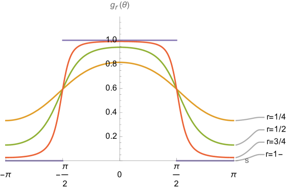
In this case, the coefficient Gaussian process $\{\xi_{k}\}_{k\geq 0}$ exhibits long-range correlation. Indeed, it is known that a stationary Gaussian process $\{\xi_{k}\}_{k\in\mathbb{Z}}$ is purely-nondeterministic if and only if $F(ds)$ is absolutely continuous and its density $f(s)=F(ds)/ds$ satisfies $\int_{-\pi}^{\pi}\log f(s)ds>-\infty$, which clearly fails in this case. This example is also discussed in [29, Example 2.4].

From (2.3), the covariance kernel is given as the harmonic extension of the spectral density $f(s)$, i.e., for $z=re^{i\theta}$,

$\displaystyle K_{F}(z,z)$ $\displaystyle=\frac{1}{1-r^{2}}\frac{1}{2\pi}\int_{-\pi/2}^{\pi/2}P(r,\theta-t)dt$
$\displaystyle=\frac{1}{1-r^{2}}\left\{\frac{1}{2}+\frac{1}{\pi}\arctan\Big{(}\frac{2r}{1-r^{2}}\cos\theta\Big{)}\right\},$

where $P(r,\theta)$ is the Poisson kernel in (2.4). Here we carefully used the formula

$$\frac{d}{dt}2\arctan\left(\frac{1+r}{1-r}\tan\frac{t}{2}\right)=P(r,t).$$

By using (2.5), it is not difficult to see that

$\displaystyle\rho_{1}(re^{i\theta})$ $\displaystyle=\frac{1}{\pi(1-r^{2})^{2}}\times\left\{1-\frac{\frac{\left(1-r^{2}\right)^{2}}{1+2r^{2}\cos 2\theta+r^{4}}}{\left(\frac{\pi}{2}+\arctan\left(\frac{2r}{1-r^{2}}\cos\theta\right)\right)^{2}}\right\}$
$\displaystyle=\begin{cases}\frac{1}{\pi(1-r^{2})^{2}}\times\displaystyle\left\{1-\frac{1}{4\pi\cos^{2}\theta}(1-r^{2})^{2}\right\}+O((1-r^{2})^{3})&\theta\in(-\frac{\pi}{2},\frac{\pi}{2})\\[5.69054pt] \displaystyle 1-(\frac{2}{\pi})^{2}&\theta=\pm\frac{\pi}{2}\\[5.69054pt] \displaystyle\frac{1}{12\cos^{2}\theta}(1-r^{2})^{2}+O((1-r^{2})^{3})&\theta\in(-\pi,\pi)\setminus[-\frac{\pi}{2},\frac{\pi}{2}],\end{cases}$

as $r\to 1$. See Fig. 2 for $\rho_{1}(re^{i\theta})$.

Refer to caption
Figure 2. The graph of $g_{r}(\theta)=\pi(1-r^{2})^{2}\rho_{1}(re^{i\theta})$ for $r=1/4,1/2,3/4,1-$. The common intersection point of all the graphs is $1-(2/\pi)^{2}\approx 0.594715$ at $\theta=\pm\pi/2$.

While the expected number of zeros is $O((1-r^{2})^{-2})$ as $r\to 1$, it is extremely small; indeed, $O(1)$ in the direction of $e^{i\theta}$ with $\theta\in(-\pi,\pi)\setminus[-\pi/2,\pi/2]$, where the spectral density vanishes. This implies that the boundary behavior of the $1$-intensity of zeros heavily depends on the boundary value of the spectral density [29]. See the right panel in Fig. 1.

For the simulation shown in the right panel of Fig. 1, we approximate $X_{F}(z)$ using the diagonalization of the coefficient Gaussian process. We take the unique positive-definite square root $A$ of the positive-definite, symmetric matrix $K_{F}=(\gamma(i-j))_{i,j=0}^{\infty}$, i.e., $K_{F}=A^{2}$. Then, $\Xi=\{\xi_{i}\}_{i=0}^{\infty}$ can be constructed as follows:

$$\xi_{i}:=\sum_{j=0}^{\infty}A_{ij}\zeta_{j},$$

where $\{\zeta_{j}\}_{j=0}^{\infty}$ are i.i.d complex standard normal. Here, we approximate $X_{F}(z)=\sum_{i=0}^{\infty}\xi_{i}z^{i}$ by the double sum

$$X_{F}^{(N)}(z)=\sum_{i=0}^{N}\left(\sum_{j=0}^{N}A_{ij}\zeta_{j}\right)z^{i}=\sum_{j=0}^{N}\zeta_{j}\left(\sum_{i=0}^{N}A_{ij}z^{i}\right).$$

It is easy to see that the covariance kernel is given by

$$K_{F}^{(N)}(z,z)=\sum_{i,k=0}^{N}(A|_{[0,N]}^{2})_{ik}z^{i}\bar{z}^{k},$$

where $A|_{[0,N]}$ is the submatrix whose rows and columns are restricted on the indices $\{0,1,\dots,N\}$. Let $P^{(N)}$ be the projection operator that maps $(x_{0},x_{1},\dots)$ to $(x_{0},x_{1},\dots,x_{N},0,0,\dots)$, i.e., the restriction onto the set $\{0,1,\dots,N\}$. Then,

$$K_{F}^{(N)}(z,z)=\langle P^{(N)}AP^{(N)}AP^{(N)}\mathbf{z},\mathbf{z}\rangle=\|P^{(N)}AP^{(N)}\mathbf{z}\|^{2}\leq\|A\mathbf{z}\|^{2}=K_{F}(z,z),$$

where $\mathbf{z}=\{1,z,z^{2},\dots\}$ with $z\in\mathbb{D}$, from which we can see that $\sup_{N}E[|X_{F}^{(N)}(z)|^{2}]=\sup_{N}K_{F}^{(N)}(z,z)$ is locally integrable. Since $K_{F}^{(N)}(z,w)\to K_{F}(z,w)$ for every $z,w\in\mathbb{D}$, by Propositions 2.2 and 2.3, we have that $\{X_{F}^{(N)}(z)\}_{z\in\mathbb{D}}$ converges in law to $\{X_{F}(z)\}_{z\in\mathbb{D}}$, and hence the zero process $\mathcal{Z}_{X_{F}^{(N)}}$ converges in law to $\mathcal{Z}_{X_{F}}$ as $N\to\infty$.

The zeros of $X_{F}^{(N)}(z)$ were computed repeatedly for $N=200$ as shown in Fig. 3. In the left half-plane, the zeros are almost evenly distributed near the unit circle, whereas in the right half-plane, the zeros are more randomly distributed, similar to the previous examples. On average, the number of zeros inside and outside the unit disk is approximately equal both in the right and left half-plane.

Refer to caption
Figure 3. The zeros of $X_{F}^{(N)}(z)$ were computed for $N=200$. The red points indicate zeros inside the unit disk, while the blue points indicate zeros outside the unit disk. The patterns of red and blue points seem to random.
Refer to caption
Figure 4. The zeros of $X_{F}^{(100)}(z)$ are computed $10,000$ times. The left (resp. right) panel shows the number of zeros inside the unit disk in the left-half (resp. right-half) plane.

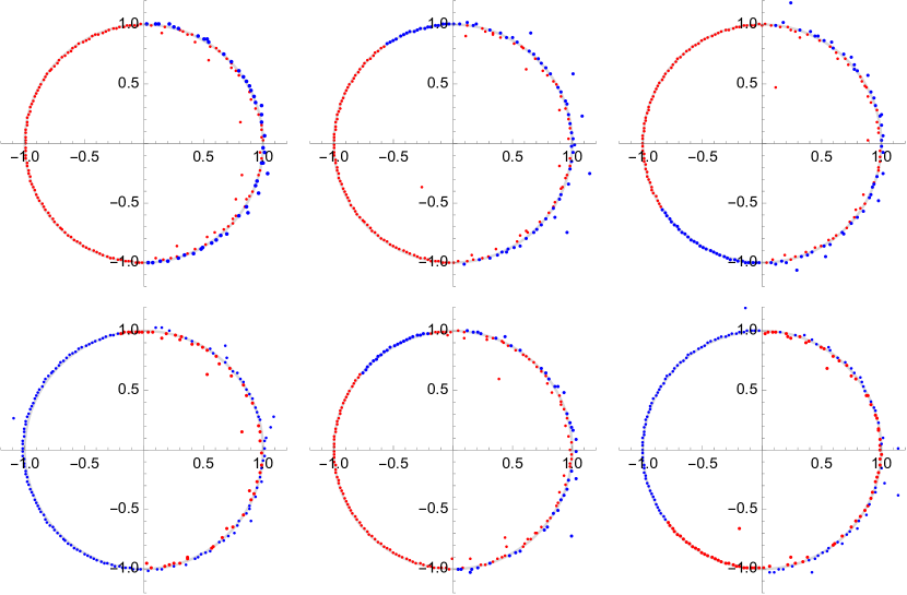
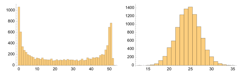
However, the variance for the left-half plane appears to be larger than that for the right half-plane. To see this situation further, we computed the zeros of $X_{F}^{(100)}(z)$ $10,000$ times. The left (resp. right) panel of Fig. 4 shows the number of zeros inside the unit disk in the left-half (resp. right-half) plane. The central limit theorem seem to hold for the number of zeros inside $\mathbb{D}$ in the right-half plane. On the other hand, the number of zeros inside $\mathbb{D}$ in the left-half plane behaves differently.

4. Spectral representation of $n$-point correlation function

Using the Edelman-Kostlan formula, the 1-correlation function is expressed in terms of the covariance kernel. In Section 2, we provided an integral representation (2.5) of the $1$-correlation function involving the spectral measure $F(dt)$. In this section, we extend this approach to derive an integral representation of the $n$-point correlation function for the zeros of the GAF, also in terms of the spectral measure $F(dt)$.

We define the conditional kernel $K^{a}(z,w)$ by

$$K^{a}(z,w)=K(z,w)-\frac{K(z,a)K(a,w)}{K(a,a)}=\frac{1}{K(a,a)}\begin{vmatrix}K(z,w)&K(z,a)\\ K(a,w)&K(a,a)\end{vmatrix}$$ (4.1)

whenever $K(a,a)>0$, and inductively, $K^{a_{1},a_{2},\dots,a_{n}}(z,w)=(K^{a_{1},a_{2},\dots,a_{n-1}})^{a_{n}}(z,w)$. Note that $K^{a_{1},a_{2},\dots,a_{n}}(z,w)$ can also be represented as the ratio of determinants, i.e.,

$$K^{a_{1},a_{2},\dots,a_{n}}(z,w)=\Big{(}\det(K(a_{j},a_{k}))_{j,k=1}^{n}\Big{)}^{-1}\det(K(a_{j},a_{k}))_{j,k=0}^{n}\Big{|}_{\text{$a_{0}=z$ or $w$}},$$ (4.2)

where “$a_{0}=z$ or $w$” means that $K(a_{0},a_{k})=K(z,a_{k})$ and $K(a_{j},a_{0})=K(a_{j},w)$ for $j,k=1,2,\dots,n$, and $K(a_{0},a_{0})=K(z,w)$. When we denote by $\mathcal{H}_{K}$ the reproducing kernel Hilbert space corresponding to $K$, $\mathcal{H}_{K^{a_{1},\dots,a_{n}}}$ is given by

$$\mathcal{H}_{K^{a_{1},\dots,a_{n}}}=\{f\in\mathcal{H}_{K}:f(a_{j})=0\text{ for $j=1,2\dots,n$}\}.$$

This corresponds to the conditional GAF $\{X(z)\}_{z\in\mathbb{D}}$ given that $X(a_{1})=X(a_{2})=\cdots=X(a_{n})=0$.

Now we recall the following formula for the $n$-point correlation function of the zeros of GAF (cf. [15, Corollary 3.4.2]). For our convenience, we use the same formula in a slightly different form as presented in [28, Proposition 6.1],

Proposition 4.1.

The $n$-point correlation function of the zeros of GAF with covariance kernel $K(z,w)$ is given by the formula

$$\rho_{n}(z_{1},z_{2},\dots,z_{n})=\frac{\operatorname{per}(\partial_{z}\partial_{\bar{w}}K^{z_{1},z_{2},\dots,z_{n}}(z_{j},z_{k}))_{j,k=1}^{n}}{\det(\pi K(z_{j},z_{k}))_{j,k=1}^{n}}$$

for distinct $z_{1},z_{2},\dots,z_{n}\in D$ with $\det(K(z_{j},z_{k}))_{j,k=1}^{n}>0$, where $\operatorname{per}A$ is the permanent of an $n$ by $n$ matrix $A=(a_{jk})_{j,k=1}^{n}$ defined by

$$\operatorname{per}A=\sum_{\sigma\in\mathcal{S}_{n}}\prod_{j=1}^{n}a_{j\sigma(j)},$$

where $\mathcal{S}_{n}$ is the symmetric group of order $n$.

This formula follows from the fact that

$\displaystyle\rho_{n}(z_{1},z_{2},\dots,z_{n})$
$\displaystyle=\mathbb{E}[|X^{\prime}(z_{1})X^{\prime}(z_{2})\cdots X^{\prime}(z_{n})|^{2}\ |\ X(z_{1})=X(z_{2})=\cdots=X(z_{n})=0]$

and the second moment of the product of complex Gaussian random variables is equal to the permanent of the covariance matrix, i.e., if $Y=(Y_{1},Y_{2},\dots,Y_{n})$ is a centered Gaussian vector with covariance matrix $K=(K_{jk})_{j,k=1}^{n}$, then

$$\mathbb{E}[|Y_{1}Y_{2}\cdots Y_{n}|^{2}]=\operatorname{per}K.$$

For $\mathbf{a}=(a_{1},\dots,a_{n})$, let $V(\mathbf{a})$ be the Vandermonde determinant defined by

$$V(\mathbf{a})=V(a_{1},a_{2},\dots,a_{n}):=\det(a_{j}^{k-1})_{j,k=1}^{n}=\prod_{1\leq j<k\leq n}(a_{k}-a_{j}).$$

Later, we will also use it in the form

$$\prod_{j,k=1\atop{k\not=j}}^{n}(a_{k}-a_{j})=(-1)^{{n\choose 2}}V(\mathbf{a})^{2}.$$ (4.3)

We recall the Cauchy determinant identity

$$\det\Big{(}\frac{1}{1-a_{j}b_{k}}\Big{)}_{j,k=1}^{n}=V(\mathbf{a})V(\mathbf{b})\prod_{j,k=1}^{n}\frac{1}{1-a_{j}b_{k}}.$$ (4.4)

For $\mathbf{a}=(a_{1},a_{2},\dots,a_{n})$, $\mathbf{t}=(t_{1},t_{2},\dots,t_{n})$, and $\mathbf{z}=(z_{1},z_{2},\dots,z_{m})$ (possibly with different $n$ and $m$), we define

$$D(\mathbf{a},\mathbf{t})=\det(s(a_{j},t_{k}))_{j,k=1}^{n},\quad S(\mathbf{z},\mathbf{t})=\prod_{j=1}^{m}\prod_{k=1}^{n}s(z_{j},t_{k}).$$

In what follows in this section, the elements of $\mathbf{a}$ and $\mathbf{z}$ are assumed to belong to $\mathbb{D}$.

From (2.2) and the Cauchy identity (4.4), we have

$$D(\mathbf{a},\mathbf{t})=V(\mathbf{a})V(e^{-it_{1}},\dots,e^{-it_{n}})S(\mathbf{a},\mathbf{t}).$$ (4.5)
Lemma 4.2.

For $\mathbf{a}=(a_{1},a_{2},\dots,a_{n})$ and $\mathbf{t}=(t_{1},t_{2},\dots,t_{n})$, we have

$$\det(K(a_{j},a_{k}))_{j,k=1}^{n}=|V(\mathbf{a})|^{2}\mu_{\mathbf{a}}(\mathbb{T}^{n}),$$ (4.6)

where

$$\mu_{\mathbf{a}}(d\mathbf{t})=\frac{1}{n!}|V(e^{-it_{1}},e^{-it_{2}},\dots,e^{-it_{n}})|^{2}\cdot|S(\mathbf{a},\mathbf{t})|^{2}F^{\otimes n}(d\mathbf{t}).$$ (4.7)
Proof.

By (2.1) and the symmetrization of the variable $\mathbf{t}$, we see that

$\displaystyle\det(K(a_{j},a_{k}))_{j,k=1}^{n}$ $\displaystyle=\sum_{\sigma\in\mathcal{S}_{n}}\operatorname{sgn}(\sigma)\int_{\mathbb{T}^{n}}\prod_{k=1}^{n}s(a_{\sigma(k)},t_{k})\cdot\overline{\prod_{k=1}^{n}s(a_{k},t_{k})}F^{\otimes n}(d\mathbf{t})$
$\displaystyle=\int_{\mathbb{T}^{n}}\det(s(a_{j},t_{k}))_{j,k=1}^{n}\overline{\Big{(}\prod_{k=1}^{n}s(a_{k},t_{k})\Big{)}}F^{\otimes n}(d\mathbf{t})$
$\displaystyle=\frac{1}{n!}\int_{\mathbb{T}^{n}}\det(s(a_{j},t_{k}))_{j,k=1}^{n}\overline{\det(s(a_{j},t_{k}))_{j,k=1}^{n}}F^{\otimes n}(d\mathbf{t})$
$\displaystyle=\frac{1}{n!}\int_{\mathbb{T}^{n}}|D(\mathbf{a},\mathbf{t})|^{2}F^{\otimes n}(d\mathbf{t}).$

The assertion follows directly from the identity (4.5). ∎

Remark 4.3.

Let $\mathcal{U}(n)$ denote the compact Lie group of $n\times n$ unitary matrices and let $P_{n}$ be the Haar measure on it. The pair $(\mathcal{U}(n),P_{n})$ is called the circular unitary ensemble CUEn. The eigenvalues of CUEn are known to form the $n$-point DPP on $\mathbb{T}$ associated with the rank $n$ projection kernel

$$\tilde{k}_{n}(\theta,\varphi)=\sum_{k=0}^{n-1}e^{ik\theta}\overline{e^{ik\varphi}}=u(\theta)\frac{\sin\frac{n(\theta-\varphi)}{2}}{\sin\frac{\theta-\varphi}{2}}\overline{u(\varphi)}=:u(\theta)k_{n}(\theta,\varphi)\overline{u(\varphi)},$$

where $u(\theta)=e^{i(n-1)\theta/2}$ and with the background measure being the Lebesgue probability measure on $\mathbb{T}$. The probability measure on $\mathbb{T}^{n}$ with density $\mu_{\mathbf{a}}(\mathbf{t})/\mu_{\mathbf{a}}(\mathbb{T}^{n})$ can be regarded as the $n$-point DPP associated with the correlation kernel $k_{n}(\theta,\varphi)$ and the background measure

$$|S(\mathbf{a},t)|^{2}F(dt)=\Big{(}\prod_{j=1}^{n}\frac{1}{1-r_{j}^{2}}\Big{)}\Big{(}\prod_{j=1}^{n}P(r_{j},\varphi_{j}-t)\Big{)}F(dt),$$

where $a_{j}=r_{j}e^{i\varphi_{j}}$ and $P(r,\theta)$ is the Poisson kernel in (2.4). We denote this $n$-point DPP on $\mathbb{T}$ by $\mathbb{P}_{\mathbf{a}}^{(n)}$.

Lemma 4.4.

For $\mathbf{a}=(a_{1},a_{2},\dots,a_{n})$ and $\tilde{\mathbf{t}}=(t_{0},t_{1},\dots,t_{n})$,

$\displaystyle\det(K(a_{j},a_{k}))_{j,k=1}^{n}\cdot K^{a_{1},\dots,a_{n}}(z,w)$
$\displaystyle=|V(\mathbf{a})|^{2}\prod_{i=1}^{n}(z-a_{i})\overline{(w-a_{i})}\int_{\mathbb{T}^{n+1}}S(z,\tilde{\mathbf{t}})\overline{S(w,\tilde{\mathbf{t}})}\tilde{\mu}_{\mathbf{a}}(d\tilde{\mathbf{t}})$
$\displaystyle=|V(\mathbf{a})|^{2}\tilde{\mu}_{\mathbf{a}}(\mathbb{T}^{n+1})\prod_{i=1}^{n}(z-a_{i})\overline{(w-a_{i})}\cdot K_{\mathbf{a}}^{(n+1)}(z,w)$

where

$$\tilde{\mu}_{\mathbf{a}}(d\tilde{\mathbf{t}})=\frac{1}{(n+1)!}|V(e^{-it_{0}},e^{-it_{1}},\dots,e^{-it_{n}})|^{2}|S(\mathbf{a},\tilde{\mathbf{t}})|^{2}F^{\otimes(n+1)}(d\tilde{\mathbf{t}}).$$

and

$$K_{\mathbf{a}}^{(n+1)}(z,w)=\mathbb{E}_{\mathbf{a}}^{(n+1)}[S(z,\tilde{\mathbf{t}})\overline{S(w,\tilde{\mathbf{t}})}],$$

where $\mathbb{E}_{\mathbf{a}}^{(n+1)}$ is the expectation with respect to $\mathbb{P}_{\mathbf{a}}^{(n+1)}$ defined as in Remark 4.3.

Proof.

As in the previous calculation in the proof of Lemma 4.2, by (4.2), it follows that

$\displaystyle Q_{n}(z,w)$ $\displaystyle:=\det(K(a_{j},a_{k}))_{j,k=1}^{n}K^{a_{1},\dots,a_{n}}(z,w)$
$\displaystyle=\det(K(a_{j},a_{k}))_{j,k=0}^{n}\Big{|}_{\text{$a_{0}=z$ or $w$}}$
$\displaystyle=\frac{1}{(n+1)!}\int_{\mathbb{T}^{n+1}}\det(s(a_{i},t_{j}))_{i,j=0}^{n}\Big{|}_{a_{0}=z}\cdot\overline{\det(s(a_{i},t_{j}))_{i,j=0}^{n}}\Big{|}_{a_{0}=w}F^{\otimes n+1}(dt_{0}d\mathbf{t}).$

Setting $\tilde{\mathbf{a}}=(a_{0},\mathbf{a})$, by (4.4), we have

$\displaystyle\det(s(a_{j},t_{k}))_{j,k=0}^{n}\Big{|}_{a_{0}=z}$ $\displaystyle=V(\tilde{\mathbf{a}})V(e^{-it_{0}},e^{-it_{1}},\dots,e^{-it_{n}})S(\tilde{\mathbf{a}},\tilde{\mathbf{t}})\Big{|}_{a_{0}=z}$
$\displaystyle=\prod_{j=1}^{n}(a_{j}-z)\cdot V(\mathbf{a})V(e^{-it_{0}},e^{-it_{1}},\dots,e^{-it_{n}})S(z,\tilde{\mathbf{t}})S(\mathbf{a},\tilde{\mathbf{t}}).$

Hence, we obtain

$\displaystyle Q_{n}(z,w)$ $\displaystyle=\frac{1}{(n+1)!}|V(\mathbf{a})|^{2}\prod_{j=1}^{n}(z-a_{j})\overline{(w-a_{j})}$
$\displaystyle\quad\times\int_{\mathbb{T}^{n+1}}S(z,\tilde{\mathbf{t}})\overline{S(w,\tilde{\mathbf{t}})}\cdot|V(e^{-it_{0}},e^{-it_{1}},\dots,e^{-it_{n}})|^{2}|S(\mathbf{a},\tilde{\mathbf{t}})|^{2}F^{\otimes(n+1)}(d\tilde{\mathbf{t}}).$

This completes the proof. ∎

Now we compute the $n$-correlation function $\rho_{n}(\mathbf{a})$ using Proposition 4.1, Lemmas 4.2 and 4.4.

Theorem 4.5.

For pairwise distinct $\mathbf{a}=(a_{1},a_{2},\dots,a_{n})\in\mathbb{D}^{n}$,

$\displaystyle\rho_{n}(\mathbf{a})$ $\displaystyle=\frac{1}{\pi^{n}}|V(\mathbf{a})|^{2}\frac{\tilde{\mu}_{\mathbf{a}}(\mathbb{T}^{n+1})^{n}}{\mu_{\mathbf{a}}(\mathbb{T}^{n})^{n+1}}\operatorname{per}(K_{\mathbf{a}}^{(n+1)}(a_{p},a_{q}))_{p,q=1}^{n}.$
Proof.

By Lemma 4.4, we note that

$\displaystyle\partial_{z}\partial_{\bar{w}}Q_{n}(z,w))|_{z=a_{p},w=a_{q}}$
$\displaystyle=|V(\mathbf{a})|^{2}\tilde{\mu}_{\mathbf{a}}(\mathbb{T}^{n+1})\left(\prod_{i=1\atop{i\not=p}}^{n}(a_{p}-a_{i})\overline{\prod_{j=1\atop{j\not=q}}^{n}(a_{q}-a_{j})}\right)K_{\mathbf{a}}^{(n+1)}(a_{p},a_{q}).$

Then, we see that

$\displaystyle\operatorname{per}((\partial_{z}\partial_{\bar{w}}Q_{n}(z,w))|_{z=a_{p},w=a_{q}})$
$\displaystyle=\left\{|V(\mathbf{a})|^{2}\tilde{\mu}_{\mathbf{a}}(\mathbb{T}^{n+1})\right\}^{n}\sum_{\sigma\in\mathcal{S}_{n}}\prod_{p=1}^{n}\left(\prod_{i=1\atop{i\not=p}}^{n}(a_{p}-a_{i})\overline{\prod_{j=1\atop{j\not=\sigma(p)}}^{n}(a_{\sigma(p)}-a_{j})}\right)K_{\mathbf{a}}^{(n+1)}(a_{p},a_{\sigma(p)})$
$\displaystyle=|V(\mathbf{a})|^{2n+4}\tilde{\mu}_{\mathbf{a}}(\mathbb{T}^{n+1})^{n}\operatorname{per}\big{(}K_{\mathbf{a}}^{(n+1)}(a_{p},a_{q})_{p,q=1}^{n}\big{)}.$

Here, we used (4.3) in the second equality. Therefore, by Lemma 4.2, we obtain

$\displaystyle\rho_{n}(\mathbf{a})$ $\displaystyle=\frac{\operatorname{per}((\partial_{z}\partial_{\bar{w}}K^{a_{1},\dots,a_{n}}(z,w))|_{z=a_{p},w=a_{q}})}{\det(\pi K)}=\frac{\operatorname{per}((\partial_{z}\partial_{\bar{w}}Q_{n}(z,w))|_{z=a_{p},w=a_{q}})}{\pi^{n}(\det K)^{n+1}}$
$\displaystyle=\frac{|V(\mathbf{a})|^{2}\tilde{\mu}_{\mathbf{a}}(\mathbb{T}^{n+1})^{n}}{\pi^{n}\mu_{\mathbf{a}}(\mathbb{T}^{n})^{n+1}}\operatorname{per}(K_{\mathbf{a}}^{(n+1)}(a_{p},a_{q})_{p,q=1}^{n}).$

This is the desired formula. ∎

Remark 4.6.

Theorem 4.5 shows that the $n$-correlation function includes the factor of squared Vandermonde determinant $|V(\mathbf{a})|^{2}$. For $\mathbf{a}=(a_{1},\dots,a_{n})$, we consider a monic polynomial $p(z)=\prod_{k=1}^{n}(z-a_{k})$ and suppose it has the coeffcients $e_{k},k=0,1,\dots,n-1$, i.e., $p(z)=\sum_{k=0}^{n}e_{k}z^{k}$ with $e_{n}=1$. Then the transformation $T:\mathbb{C}^{n}\to\mathbb{C}^{n}$ defined by $T(a_{1},a_{2},\dots,a_{n})=(e_{n-1},e_{n-2},\dots,e_{0})$ has Jacobian determinant $|V(\mathbf{a})|^{2}$ (cf. [15]), which is reflected in the theorem. See also [23, 13].

4.1. Reproducing formula

We present a multi-dimensional reproducing formula of the Cauchy type, which appears in the computation in Section 4.2.

Lemma 4.7.

Let

$$C(\mathbf{z},\mathbf{a}):=\prod_{k=1}^{n}\prod_{j=1}^{n}\frac{1}{z_{k}-a_{j}}.$$

Then, for an analytic function $Q(\mathbf{z})$ that is symmetric in its variables,

$$\left(\frac{1}{2\pi i}\right)^{n}\oint_{C^{n}}V(\mathbf{z})^{2}C(\mathbf{z},\mathbf{a})Q(\mathbf{z})\prod_{k=1}^{n}dz_{k}=(-1)^{{n\choose 2}}n!\cdot Q(\mathbf{a}),$$ (4.8)

and for pairwise distinct $\mathbf{a}=(a_{1},\dots,a_{n})$,

$\displaystyle\left(\frac{1}{2\pi i}\right)^{n}\oint_{C^{n}}V(\mathbf{z})^{2}C(\mathbf{z},\mathbf{a})Q(\mathbf{z})\prod_{k=1}^{n}\frac{dz_{k}}{z_{k}}$
$\displaystyle=(-1)^{{n\choose 2}}n!\cdot\prod_{j=1}^{n}\frac{1}{a_{j}}\cdot\Big{\{}Q(\mathbf{a})-\sum_{p=1}^{n}\prod_{k=1\atop{k\not=p}}^{n}\frac{a_{k}}{a_{k}-a_{p}}Q(0,\mathbf{a}^{(p)})\Big{\}},$ (4.9)

where $C=\{z\in\mathbb{C}:|z|=1\}$ and $\mathbf{a}^{(p)}=(a_{1},\dots,a_{p-1},a_{p+1},\dots,a_{n})$.

Proof.

Due to the presence of the Vandermonde term, the residue is zero unless the points $(z_{1},z_{2},\dots,z_{n})$ are all distinct and form a permutation of $\{a_{1},\dots,a_{n}\}$. Since the integral is symmetric in $(z_{1},z_{2},\dots,z_{n})$, it suffices to consider the residue at $(z_{1},z_{2},\dots,z_{n})=(a_{1},a_{2},\dots,a_{n})$ and multiply it by $n!$. The residue is given by $\displaystyle V(\mathbf{a})^{2}\prod_{k=1\atop{k\not=j}}^{n}(a_{k}-a_{j})^{-1}Q(\mathbf{a})$ and thus, using (4.3), we obtain (4.8).

Similarly, the residue is zero unless the points $(z_{1},z_{2},\dots,z_{n})$ are all distinct and form a permutation of $\{0,a_{1},\dots,a_{n}\}\setminus\{a_{p}\}$ for some $p=1,2,\dots,n$. Since the integral is symmetric in $(z_{1},z_{2},\dots,z_{n})$, it suffices to consider the residue at $\mathbf{z}=\mathbf{a}$ or $\mathbf{z}=(0,\mathbf{a}^{(p)})$ for $p=1,2,\dots,n$ and multiply it by $n!$. For $\mathbf{z}=\mathbf{a}$, the first term in (4.9) is obtained in the same manner as above with the extra term $\prod_{k=1}^{n}1/a_{k}$. Since $\displaystyle V(0,\mathbf{a}^{(p)})=(\prod_{j=1\atop{j\not=p}}^{n}a_{j})V(\mathbf{a}^{(p)})$, the residue at $\mathbf{z}=(0,\mathbf{a}^{(p)})$ is given by

$\displaystyle\mathrm{Res}_{\mathbf{z}=(0,\mathbf{a}^{(p)})}$ $\displaystyle=(\prod_{j=1\atop{j\not=p}}^{n}a_{j})^{2}V(\mathbf{a}^{(p)})^{2}\cdot\prod_{j=1}^{n}\frac{1}{-a_{j}}\cdot\prod_{k=1\atop{k\not=p}}^{n}\prod_{j=1\atop{j\not=k}}^{n}\frac{1}{a_{k}-a_{j}}\cdot\prod_{k=1\atop{k\not=p}}^{n}\frac{1}{a_{k}}\cdot Q(0,\mathbf{a}^{(p)})$
$\displaystyle=(-1)^{{n\choose 2}+1}\prod_{j=1}^{n}\frac{1}{a_{j}}\prod_{k=1\atop{k\not=p}}^{n}\frac{a_{k}}{a_{k}-a_{p}}\cdot Q(0,\mathbf{a}^{(p)}).$

Therefore, we obtain (4.9). ∎

4.2. The case $F(dt)=dt/(2\pi)$

Let us consider the i.i.d. case, i.e., $F(dt)=dt/(2\pi)$ and $X_{F}(z)=X_{\mathrm{hyp}}(z)$. In the following lemma, by a slight abuse of notation, we write $S(\mathbf{z},\mathbf{w})=\prod_{j,k=1}^{n}s(z_{j},w_{k})=\prod_{j,k=1}^{n}(1-z_{j}\bar{w}_{k})^{-1}$ using the same symbol $S$ for the Szegő kernel $S(\mathbf{z},\mathbf{t})$.

Lemma 4.8.

Suppose $F(dt)=dt/(2\pi)$. Then,

$$\mu_{\mathbf{a}}(\mathbb{T}^{n})=\tilde{\mu}_{\mathbf{a}}(\mathbb{T}^{n+1})=S(\mathbf{a},\mathbf{a}),\quad K_{\mathbf{a}}^{(n+1)}(z,w)=S(z,w)S(z,\mathbf{a})\overline{S(w,\mathbf{a})}.$$
Proof.

By (4.7), the definition of $\mu_{\mathbf{a}}$, we see that

$\displaystyle n!\mu_{\mathbf{a}}(\mathbb{T}^{n})$ $\displaystyle=\int_{\mathbb{T}^{n}}|V(e^{-it_{1}},\cdots,e^{-it_{n}})|^{2}\prod_{k=1}^{n}\prod_{j=1}^{n}\left|\frac{1}{1-a_{j}e^{-it_{k}}}\right|^{2}\prod_{k=1}^{n}\frac{dt_{k}}{2\pi}$
$\displaystyle=\left(\frac{1}{2\pi i}\right)^{n}\oint_{C^{n}}|V(z_{1}^{-1},\cdots,z_{n}^{-1})|^{2}\prod_{k=1}^{n}\prod_{j=1}^{n}\left|\frac{1}{1-a_{j}z_{k}^{-1}}\right|^{2}\prod_{k=1}^{n}\frac{dz_{k}}{z_{k}}$
$\displaystyle=(-1)^{{n\choose 2}}\left(\frac{1}{2\pi i}\right)^{n}\oint_{C^{n}}V(\mathbf{z})^{2}C(\mathbf{z},\mathbf{a})S(\mathbf{z},\mathbf{a})\prod_{k=1}^{n}dz_{k},$

where we used $\bar{z}_{k}=z_{k}^{-1}$ on $C$ and the following identity:

$$V(z_{1}^{-1},\cdots,z_{n}^{-1})=(-1)^{{n\choose 2}}\frac{V(z_{1},\cdots,z_{n})}{(z_{1}\cdots z_{n})^{n-1}}.$$

Therefore, by (4.8), we have $\mu_{\mathbf{a}}(\mathbb{T}^{n})=S(\mathbf{a},\mathbf{a})$.

Similarly as above, setting $\tilde{\mathbf{z}}=(z_{0},z_{1},\dots,z_{n})$ and $\tilde{\mathbf{a}}_{z}=(z,\mathbf{a})=(z,a_{1},\dots,a_{n})$ and using (4.8), we have

$\displaystyle\tilde{\mu}_{\mathbf{a}}(\mathbb{T}^{n+1})K_{\mathbf{a}}^{(n+1)}(z,w)$
$\displaystyle=\int_{\mathbb{T}^{n+1}}S(z,\tilde{\mathbf{t}})\overline{S(w,\tilde{\mathbf{t}})}\tilde{\mu}_{\mathbf{a}}(d\tilde{\mathbf{t}})$
$\displaystyle=\frac{1}{(n+1)!}\int_{\mathbb{T}^{n+1}}|V(e^{-it_{0}},\cdots,e^{-it_{n}})|^{2}\prod_{k=0}^{n}\prod_{j=1}^{n}\left|\frac{1}{1-a_{j}e^{-it_{k}}}\right|^{2}$
$\displaystyle\quad\times\prod_{k=0}^{n}\frac{1}{1-ze^{-it_{k}}}\overline{\frac{1}{1-we^{-it_{k}}}}\prod_{k=0}^{n}\frac{dt_{k}}{2\pi}$
$\displaystyle=(-1)^{{n+1\choose 2}}\frac{1}{(n+1)!}\left(\frac{1}{2\pi i}\right)^{n+1}\oint_{C^{n+1}}V(\tilde{\mathbf{z}})^{2}C(\tilde{\mathbf{z}},\tilde{\mathbf{a}}_{z})S(\tilde{\mathbf{z}},\tilde{\mathbf{a}}_{w})\prod_{k=0}^{n}dz_{k}$
$\displaystyle=S(\tilde{\mathbf{a}}_{z},\tilde{\mathbf{a}}_{w}).$

Hence, $K_{\mathbf{a}}^{(n+1)}(z,w)=S(\tilde{\mathbf{a}}_{z},\tilde{\mathbf{a}}_{w})/\tilde{\mu}_{\mathbf{a}}(T^{n+1})$. Since the left-hand side is $1$ when $z=w=0$ by the definition of $K_{\mathbf{a}}^{(n+1)}(z,w)$, we see that $\tilde{\mu}_{\mathbf{a}}(\mathbb{T}^{n+1})=S(\tilde{\mathbf{a}}_{0},\tilde{\mathbf{a}}_{0})=S(\mathbf{a},\mathbf{a})$, and thus, $K_{\mathbf{a}}^{(n+1)}(z,w)=S(z,w)S(z,\mathbf{a})\overline{S(w,\mathbf{a})}$. ∎

Now we compute the $n$-correlation function of the zeros for $X_{\mathrm{hyp}}(z)$. By Theorem 4.5 together with Lemma 4.8, we obtain

$\displaystyle\rho_{n}(\mathbf{a})$ $\displaystyle=\frac{1}{\pi^{n}}|V(\mathbf{a})|^{2}\frac{1}{S(\mathbf{a},\mathbf{a})}\operatorname{per}(S(a_{p},a_{q})S(a_{p},\mathbf{a})\overline{S(a_{q},\mathbf{a})})_{p,q=1}^{n}$
$\displaystyle=\frac{1}{\pi^{n}}|V(\mathbf{a})|^{2}S(\mathbf{a},\mathbf{a})\operatorname{per}(S(a_{p},a_{q}))_{p,q=1}^{n}$
$\displaystyle=\frac{1}{\pi^{n}}\det(S(a_{p},a_{q}))_{p,q=1}^{n}\cdot\operatorname{per}(S(a_{p},a_{q}))_{p,q=1}^{n}$
$\displaystyle=\frac{1}{\pi^{n}}\det(S(a_{p},a_{q})^{2})_{p,q=1}^{n}.$

We used the Cauchy determinant formula (4.4) for the third equality and Borchardt’s identity (see [15, Proposition 5.1.5])

$$\det\Big{(}\frac{1}{1-a_{p}b_{q}}\Big{)}_{p,q=1}^{n}\operatorname{per}\Big{(}\frac{1}{1-a_{p}b_{q}}\Big{)}_{p,q=1}^{n}=\det\Big{(}\frac{1}{(1-a_{p}b_{q})^{2}}\Big{)}_{p,q=1}^{n}$$

for the fourth equality. We recovered the fact that the zeros of $X_{\mathrm{hyp}}(z)$ is the determinantal point process associated with the Bergman kernel $S(z,w)^{2}$.

5. Concluding remarks

We have discussed GAFs corresponding to three spectral measures as examples in Section 3. In particular, for the polynomial approximation of the final example of GAFs, the zeros in the left half-plane exhibited somewhat different behavior compared to those in the right half-plane. Further detailed analysis of this phenomenon is left as a topic for future research. The integral representation of the $n$-point correlation functions in the final section is used only in the proof of the Peres-Virág theorem. It may also have potential applications in the detailed analysis of the two-point or higher order correlation functions of the zeros of GAFs, particularly for determining whether they exhibit negative correlations. Other topics such as central limit theorems [4, 19, 5], hole probability [20, 6], rigidity [13, 12], and hyperuniformity [14] would also be interesting to investigate in the context of our setting.

The complex autoregressive model $\mathrm{AR}(1)$ model $\{X_{t}\}_{t\in\mathbb{Z}}$ is defined as the following stochastic difference equation

$$X_{t}=zX_{t-1}+\zeta_{t}\quad(t\in\mathbb{Z})$$ (5.1)

with i.i.d. complex-valued noise. It is known that when $|z|<1$, there is a unique stationary solution given by

$$X_{t}=X_{t}(z)=\sum_{k=0}^{\infty}\zeta_{t-k}z^{k}\quad(t\in\mathbb{Z}).$$ (5.2)

If the noise $\{\zeta_{t}\}_{t\in\mathbb{Z}}$ is an i.i.d. sequence of $\{-1,1\}$-Bernoulli random variables, for each $t\in\mathbb{Z}$, the marginal $X_{t}(\lambda)$ is equal in law to the so-called Bernoulli convolution $\sum_{k=0}^{\infty}\pm\lambda^{k}$, whose distribution $\nu_{\lambda}$ is either absolutely continuous or purely singular [16] and many properties of $\nu_{\lambda}$ have been studied (cf. [34, 26]). If the noise $\{\zeta_{t}\}_{t\in\mathbb{Z}}$ is an i.i.d. sequence of standard complex normal random variables, for each $t\in\mathbb{Z}$, the marginal $\{X_{t}(z)\}_{z\in\mathbb{D}}$ is equal in law to the hyperbolic GAF $\{X_{\mathrm{hyp}}(z)\}_{z\in\mathbb{D}}$. Then $\{X_{t}\}_{t\in\mathbb{Z}}$ defines the GAF-valued stationary process and thus, for each $t$, we have the DPP-valued stationary process $\{\mathcal{Z}_{X_{t}}\}_{t\in\mathbb{Z}}$. If we replace the i.i.d. Gaussian noise with a dependent Gaussian noise, the stationary solution to (5.1) still exists when $|z|<1$ and is again given by (5.2), which defines the GAF-valued stationary process. The one-dimensional marginal $\{X_{t}(z)\}_{z\in\mathbb{D}}$ is identical in law to the one discussed earlier in this paper. It would be intriguing to explore the above-mentioned stationary GAF-valued processes and their zero processes.


Acknowledgment. A part of this study was presented at the conference “Random Matrices and Related Topics in Jeju”, held from May 6–10, 2024, on Jeju Island, Korea. The author would like to sincerely thank Sung-Soo Byun, Nam-Gyu Kang, and Kyeongsik Nam for organizing such a wonderful conference and their warm hospitality. The author was supported by JSPS KAKENHI Grant Numbers JP22H05105, JP23H01077 and JP23K25774, and also supported in part JP21H04432 and JP24KK0060.

References

  • [1] Jacques Benatar, Alexander Borichev, and Mikhail Sodin. The ‘pits effect’ for entire functions of exponential type and the Wiener spectrum. J. Lond. Math. Soc. (2), 104(3):1433–1451, 2021.
  • [2] Alexander Borichev, Alon Nishry, and Mikhail Sodin. Entire functions of exponential type represented by pseudo-random and random Taylor series. J. Anal. Math., 133:361–396, 2017.
  • [3] Alexander Borichev, Mikhail Sodin, and Benjamin Weiss. Spectra of stationary processes on $\mathbb{Z}$. In 50 years with Hardy spaces, volume 261 of Oper. Theory Adv. Appl., pages 141–157. Birkhäuser/Springer, Cham, 2018.
  • [4] Jeremiah Buckley. Fluctuations in the zero set of the hyperbolic Gaussian analytic function. Int. Math. Res. Not. IMRN, (6):1666–1687, 2015.
  • [5] Jeremiah Buckley and Alon Nishry. Gaussian complex zeroes are not always normal: limit theorems on the disc. Probab. Math. Phys., 3(3):675–706, 2022.
  • [6] Jeremiah Buckley, Alon Nishry, Ron Peled, and Mikhail Sodin. Hole probability for zeroes of Gaussian Taylor series with finite radii of convergence. Probab. Theory Related Fields, 171(1-2):377–430, 2018.
  • [7] H. Dym and H. P. McKean. Gaussian processes, function theory, and the inverse spectral problem, volume Vol. 31 of Probability and Mathematical Statistics. Academic Press [Harcourt Brace Jovanovich, Publishers], New York-London, 1976.
  • [8] Alan Edelman and Eric Kostlan. How many zeros of a random polynomial are real? Bull. Amer. Math. Soc. (N.S.), 32(1):1–37, 1995.
  • [9] Naomi D. Feldheim. Zeroes of gaussian analytic functions with translation-invariant distribution. Israel Journal of Mathematics, 195(1):317–345, 2013.
  • [10] Naomi Dvora Feldheim. Variance of the number of zeroes of shift-invariant Gaussian analytic functions. Israel J. Math., 227(2):753–792, 2018.
  • [11] Peter J Forrester. The limiting kac random polynomial and truncated random orthogonal matrices. Journal of Statistical Mechanics: Theory and Experiment, 2010(12):P12018, dec 2010.
  • [12] Subhroshekhar Ghosh and Manjunath Krishnapur. Rigidity hierarchy in random point fields: random polynomials and determinantal processes. Comm. Math. Phys., 388(3):1205–1234, 2021.
  • [13] Subhroshekhar Ghosh and Yuval Peres. Rigidity and tolerance in point processes: Gaussian zeros and Ginibre eigenvalues. Duke Math. J., 166(10):1789–1858, 2017.
  • [14] Antti Haimi, Günther Koliander, and José Luis Romero. Zeros of Gaussian Weyl-Heisenberg functions and hyperuniformity of charge. J. Stat. Phys., 187(3):Paper No. 22, 41, 2022.
  • [15] J. Ben Hough, Manjunath Krishnapur, Yuval Peres, and Bálint Virág. Zeros of Gaussian analytic functions and determinantal point processes, volume 51 of University Lecture Series. American Mathematical Society, Providence, RI, 2009.
  • [16] Bø rge Jessen and Aurel Wintner. Distribution functions and the Riemann zeta function. Trans. Amer. Math. Soc., 38(1):48–88, 1935.
  • [17] Jean-Pierre Kahane. Some random series of functions, volume 5 of Cambridge Studies in Advanced Mathematics. Cambridge University Press, Cambridge, second edition, 1985.
  • [18] Makoto Katori and Tomoyuki Shirai. Zeros of the i.i.d. Gaussian Laurent series on an annulus: weighted Szego kernels and permanental-determinantal point processes. Comm. Math. Phys., 392(3):1099–1151, 2022.
  • [19] Avner Kiro and Alon Nishry. Fluctuations for zeros of Gaussian Taylor series. J. Lond. Math. Soc. (2), 104(3):1172–1203, 2021.
  • [20] Manjunath Krishnapur. Overcrowding estimates for zeroes of planar and hyperbolic Gaussian analytic functions. J. Stat. Phys., 124(6):1399–1423, 2006.
  • [21] Manjunath Krishnapur. From random matrices to random analytic functions. Ann. Probab., 37(1):314–346, 2009.
  • [22] Sho Matsumoto and Tomoyuki Shirai. Correlation functions for zeros of a Gaussian power series and Pfaffians. Electron. J. Probab., 18:no. 49, 18, 2013.
  • [23] F. Nazarov and M. Sodin. Correlation functions for random complex zeroes: strong clustering and local universality. Comm. Math. Phys., 310(1):75–98, 2012.
  • [24] Kohei Noda and Tomoyuki Shirai. Expected number of zeros of random power series with finitely dependent Gaussian coefficients. J. Theoret. Probab., 36(3):1534–1554, 2023.
  • [25] Raymond E. A. C. Paley and Norbert Wiener. Fourier transforms in the complex domain, volume 19 of American Mathematical Society Colloquium Publications. American Mathematical Society, Providence, RI, 1987. Reprint of the 1934 original.
  • [26] Yuval Peres, Wilhelm Schlag, and Boris Solomyak. Sixty years of Bernoulli convolutions. In Fractal geometry and stochastics, II (Greifswald/Koserow, 1998), volume 46 of Progr. Probab., pages 39–65. Birkhäuser, Basel, 2000.
  • [27] Yuval Peres and Bálint Virág. Zeros of the i.i.d. Gaussian power series: a conformally invariant determinantal process. Acta Math., 194(1):1–35, 2005.
  • [28] Tomoyuki Shirai. Limit theorems for random analytic functions and their zeros. In Functions in number theory and their probabilistic aspects, volume B34 of RIMS Kôkyûroku Bessatsu, pages 335–359. Res. Inst. Math. Sci. (RIMS), Kyoto, 2012.
  • [29] Tomoyuki Shirai. The density of zeros of random power series with stationary complex gaussian coefficients, arXiv:2501.02586.
  • [30] Tomoyuki Shirai and Yoichiro Takahashi. Fermion process and Fredholm determinant. In Proceedings of the Second ISAAC Congress, Vol. 1 (Fukuoka, 1999), volume 7 of Int. Soc. Anal. Appl. Comput., pages 15–23. Kluwer Acad. Publ., Dordrecht, 2000.
  • [31] Tomoyuki Shirai and Yoichiro Takahashi. Random point fields associated with certain Fredholm determinants. I. Fermion, Poisson and boson point processes. J. Funct. Anal., 205(2):414–463, 2003.
  • [32] M. Sodin. Zeros of Gaussian analytic functions. Math. Res. Lett., 7(4):371–381, 2000.
  • [33] Mikhail Sodin and Boris Tsirelson. Random complex zeroes. I. Asymptotic normality. Israel J. Math., 144:125–149, 2004.
  • [34] Boris Solomyak. On the random series $\sum\pm\lambda^{n}$ (an Erdos problem). Ann. of Math. (2), 142(3):611–625, 1995.
  • [35] A. Soshnikov. Determinantal random point fields. Uspekhi Mat. Nauk, 55(5(335)):107–160, 2000.