Deep Networks are Reproducing Kernel Chains
Abstract
Identifying an appropriate function space for deep neural networks remains a key open question. While shallow neural networks are naturally associated with Reproducing Kernel Banach Spaces (RKBS), deep networks present unique challenges. In this work, we extend RKBS to chain RKBS (cRKBS), a new framework that composes kernels rather than functions, preserving the desirable properties of RKBS. We prove that any deep neural network function is a neural cRKBS function, and conversely, any neural cRKBS function defined on a finite dataset corresponds to a deep neural network. This approach provides a sparse solution to the empirical risk minimization problem, requiring no more than neurons per layer, where is the number of data points.
keywords: Neural networks, Reproducing Kernel Banach Spaces, Representer Theorem
1 Introduction
While deep neural networks have proven very powerful for many machine learning problems, a fundamental understanding of such methods is still being developed. A key open question is which function space is appropriate for deep neural networks.
For shallow neural networks, appropriate spaces are Reproducing Kernel Banach Spaces (RKBS). A well-known example is the Barron space (E et al., 2020; Spek et al., 2023). Such RKBS share many of the properties of the widely successful Reproducing Kernel Hilbert Spaces (RKHS). Desirable properties include their reproducing properties through their kernel, their sparsity through the representer theorem and their concise description (Bartolucci et al., 2023). An appropriate space for deep networks should preferably have these properties as well, and be a Banach space for all commonly used activation functions.
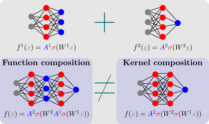
The key observation is that deep networks are not compositions of shallow networks. As seen in Figure 1, matching one network’s output with another network’s input introduces an extra linear layer, which is not present in a conventional deep network construction. Instead, via kernel composition the hidden layers are matched directly.
We use this intuition to construct our RKBS for deep networks, where instead of composing the functions of shallow RKBS, we only compose their kernels. This allows all the desirable properties of the shallow neural network spaces to be carried over and some of these to be strengthened.
In this paper, we introduce a constructive method for composing kernels of RKBSs, which we call kernel chaining. A special subclass called neural chain RKBS (cRKBS) represents neural networks: Any deep neural network is a neural cRKBS function, and any neural cRKBS function over a finite number of data points is a deep neural network. We show that these chain spaces satisfy a representer theorem, in which the sparse solution has in each layer at most as many neurons as the number of data points.
1.1 Related work
Deep networks and their corresponding spaces can be grouped into three categories. Before discussing these, we introduce foundational related work about shallow networks.
1.1.1 Shallow neural networks
Reproducing Kernel Hilbert Spaces (RKHS) are Hilbert spaces with the extra requirement that the point evaluations are bounded linear functionals. These point evaluations are linked to a kernel function through the Riesz-Fréchet representation theorem. This allows function evaluations to be written as an inner product of the kernel and the function itself. There is a unique link between the RKHS and its kernel in the sense that every RKHS has a unique kernel and every kernel uniquely defines a RKHS (Aronszajn, 1950). An important result in RKHS theory is the representer theorem. This states that the regularized minimization problem of finding the best fitting function in the RKHS given some data points has a sparse solution. This turns the infinite-dimensional minimization problem over the whole RKHS into a finite-dimensional one with dimension bounded by the number of samples, which can then be solved using a standard least squares approach.
Shallow neural networks correspond to RKHS in both the random feature limit and the lazy training limit. In the random feature limit, the hidden-layer parameters are subsampled from a particular probability distribution , and then the output layer takes a linear combination (Rahimi and Recht, 2007). If we however consider infinite linear coefficients , we get functions of an RKHS
| (1.1) |
The kernel of this RKHS depends on both the nonlinearity in the network and the particular parameter distribution. This interpretation has strong connections with Gaussian processes, and thus this limit is also called the GP-limit (Hanin, 2023). In the lazy training limit, the key observation is that the hidden-layer parameters don’t change much during training for sufficiently large networks and randomised initializations. Hence, the networks can be approximated by a linearization around such an initialization. These linearizations are elements of a RKHS with a kernel depending on both the gradient and the random initialization. This kernel is called the Neural Tangent Kernel (NTK), and thus this limit is also called the NTK-limit (Jacot et al., 2020).
Neither the random feature limit nor the lazy training limit captures the key aspects of neural networks (Chizat et al., 2019; Woodworth et al., 2020). In particular, a RKHS seems to be too small to have the right adaptability seen in neural networks (Bach, 2017). Four major research directions can be seen as extensions to the RKHS theory. These are the extended RKHS (eRKHS), variational splines, Reproducing Kernel Banach Spaces (RKBS) and the Barron spaces.
The extended RKHS is our term for the asymmetric kernel RKHS and the Hyper-RKHS (He et al., 2022, 2024; Liu et al., 2021). The main idea is to split the problem into two pieces: First, you determine a suitable kernel from a potentially infinite set of kernels for your RKHS and then determine the right function from the RKHS corresponding to this kernel. The resulting function spaces are still RKHS.
For the variational splines, the main idea is that ReLU functions are examples of splines (Parhi and Nowak, 2021). Using classical spline theory, a function space for neural networks can be constructed that has a similar representer theorem. A benefit of this approach is that the norm can be defined without making references to the weights of the network. A downside of this approach is that it does not work for all activation functions.
Instead of a fixed distribution to sample the weights, the Barron space considers all possible probability distributions that satisfy a growth limit (E et al., 2020)
| (1.2) |
Here, the growth limit is imposed to ensure the integral is well-posed when is Lipschitz. The formulation implies that Barron space is a Banach space isomorphic to a quotient over growth-limited Radon measures with bounded point evaluations (E. and Wojtowytsch, 2022). The space is not an RKHS, but a union of infinitely many RKHS (E et al., 2022; Spek et al., 2023). On compact domains, Barron spaces embed into and spaces (E. and Wojtowytsch, 2022; E et al., 2022) and functions in the space can be approximated by finite width neural networks in and with bound scaling proportionally to the inverse square root of the width of the network (E et al., 2020). Moreover, their duality structure is well-understood (Spek et al., 2023) and their dependence on the activation function characterized (Heeringa et al., 2024b; Li et al., 2020; Caragea et al., 2020). They satisfy a representer theorem (Parhi and Nowak, 2021; Bartolucci et al., 2023), but the finite-dimensional problem is now a non-convex optimisation problem and can’t be solved by a least-squares approach like RKHS. For ReLU, the corresponding Barron space agrees with the variational spline function space (Bartolucci et al., 2023).
RKBSs are the Banach analogue to RKHSs in the sense that they are Banach spaces of functions with bounded point evaluations (Zhang et al., 2009; Lin et al., 2022). When RKBSs are not Hilbert spaces, they don’t have access to the Riesz-Fréchet representation theorem for Hilbert spaces. This breaks the symmetry between primal and dual but allows for larger and more expressive function spaces. RKBSs always come in RKBS pairs: an RKBS over and an RKBS over with a non-degenerate pairing between them. The kernel is a scalar function of and . For an RKHS , and . The archetypical example of a non-Hilbertian RKBS is the space of continuous functions on a compact domain with the supremum norm. The Barron spaces (and thus also the variational splines) are instances of neural RKBSs (Spek et al., 2023), a subclass of the integral RKBSs. Results for Barron spaces carry over to the neural RKBS, and several have extensions to the vector-valued case (Bartolucci et al., 2023; Parhi and Nowak, 2021; Shenouda et al., 2024; Spek et al., 2023) and some have extensions to integral RKBSs considering different pairings than the measures with the (growth-limited) continuous functions, like ones based on Lizorkin distributions or Kantorovich-Rubinstein norms (Neumayer and Unser, 2023; Bartolucci et al., 2024a).
1.1.2 Deep neural networks
As mentioned, the approaches for deep networks can be grouped into three categories: the generalized Barron spaces, the hierarchical spaces and the bottlenecked spaces. These three categories are extensions to the directions introduced under shallow neural networks before.
The generalized Barron spaces category consists of the neural tree spaces E and Wojtowytsch (2020), a direct extension of the Barron spaces. These spaces are layered, with each layer defined based on the previous one, branching out in a tree-like fashion. The first layer is a standard Barron space. The next layer is constructed by integrating over the unit ball of functions of the previous layer, i.e. the functions are of the form
| (1.3) |
with a function from the neural tree spaces with one less depth. The neural tree spaces consist of Lipschitz functions, have bounded point evaluations, and satisfy a direct approximation theorem as well as an inverse approximation theorem. Thereby extending several of their previously proven results from Barron spaces over to the neural tree spaces. The representer theorem shows that a sparse solution with at most neurons for layer exists, for a total of at most parameters.
The hierarchical spaces category consists of the Neural Hilbert Ladder (NHL) (Chen, 2024), a direct extension of RKHS with hierarchical kernels (Huang et al., 2023). They have now multiple RKHS arranged in a layerwise fashion, each with multiple different choices of kernel. These follow a similar approach as the neural tree spaces, in the sense that the first kernel is given by
| (1.4) |
and the later kernels are given
| (1.5) |
with the integral over the functions from the NHL with one less depth. To define the kernel in (1.5), a choice has to be made for the probability measure . Each sequence of defines a hierarchical RKHS. The -NHL functions space consists of functions with a finite complexity,
| (1.6) |
with the Hilbert spaces in the infimum being constructed using a sequence of probability measures and a weight for that space. The is only a quasi-norm when is homogeneous due to its otherwise unbounded quasi-triangle constant. For , the NHL is equivalent to a Barron space since the complexity agrees then with the Barron norm.
The bottle-necked spaces consist of all approaches in which shallow neural networks are composed function-wise. The non-Hilbertian approaches within this category are the deep RKBSs and the deep variational splines (Bartolucci et al., 2024b; Parhi and Nowak, 2022). In the former, they are compositions of vector-valued variational spline spaces and in the latter, the functions are compositions of vector-valued RKBSs. In both cases, the resulting set of functions is not a normed vector space and is dependent on the intermediate sets. The deep variational splines are restricted to using the rectifier power unit (RePU), the higher order version of ReLU, as an activation function, whereas the deep RKBSs have no such restriction. The networks in the deep variational splines have skip connections, whereas the networks in the deep RKBSs do not. In the representer theorem, the former has neural networks with alternating finite and uncountable layers, whereas the latter has networks with alternating countable and uncountable layers. The difference in construction results in different scaling in the number of parameters in the representer theorem, with the former having at most total parameters for a network with predetermined intermediate sizes and the latter having at most total parameters for a network for some set of intermediate sizes satisfying .
The generalized Barron spaces are limited to ReLU, their kernel structure is unknown and their representer theorem has a solution growing exponentially in width with increasing depth. The hierarchical spaces are, just like the bottle-necked spaces, no longer normed function spaces. Hence, neither of these three categories provides a function space satisfying the necessary and preferred properties for being an appropriate function space for deep neural networks. Therefore, the key question is still open.
1.2 Our contribution
In this work, we introduce a constructive method for composing kernels of RKBSs which results in chain RKBSs (cRKBS). These spaces are distinct from deep compositional RKBS of Bartolucci et al. (2024b) in the sense that not the functions of the respective spaces are composed but the kernels of the respective spaces. We show that cRKBS preserve the RKBS structure with a proper kernel.
Next, we make the cRKBS framework more concrete by focussing on integral RKBS, where functions are defined as integrals over either the first or second argument of the kernel with respect to some measure. In particular, we focus on kernels which are a combination of an elementwise non-linearity and an affine transformation. We call integral RKBS with such kernels neural RKBS. We develop a concise formula of the function of neural chain RKBS in terms of the functions of a neural cRKBS with one less layer.
This leads to the following main theorem of this work, which precise statement is given by Theorems 14 and 18.
Theorem 1.
Every deep neural network of depth is an element of the neural cRKBS for depth . Conversely, if we only consider data points, then all functions in a neural cRKBS are deep networks with at most hidden nodes per layer and all the weights, except the last layer, are shared.
We prove this theorem by leveraging the primal-dual relation between RKBS pairs and that the activation function acts only elementwise. This also implies that neural cRKBSs satisfy a representer theorem with sparse solutions of most hidden neurons for each layer where equal to the amount of data points, for a total of at most parameters.
2 Chain Reproducing Kernel Banach Spaces
In this section, we will start by reviewing the theory of Reproducing Kernel Banach Spaces. Afterwards, we will introduce a procedure to construct chain RKBS by composing their kernels. This is done by iteratively adding ’links’ to make a ’chain’.
2.1 Reproducing Kernel Banach Spaces
We start with a Banach space of functions on a domain mapping to the reals. This means that elements of are determined by function evaluation on , i.e. for all implies that is the zero vector. This also means that contains true functions, not function classes like in a Lebesgue space. We say that is reproducing on when point evaluation is a bounded functional.
Definition 2.
Let be a Banach space of real functions on a domain . is a Reproducing Kernel Banach space (RKBS) if, for every , there exists a
| (2.1) |
for all .
Notably, this constant is independent of . This means that the functional which evaluates functions at , denoted by , must be an element of the dual space .
The archetypical example of such an RKBS is the Banach space of continuous functions on a compact set , where the max-norm trivially satisfies the above condition. The corresponding functional here is the point measure , which is an element of the dual of the continuous functions, the space of Radon measures .
A common way of constructing different RKBSs is with a feature space and a feature map .
Theorem 3.
(Bartolucci et al., 2023, Proposition 3.3) A Banach space of functions on is reproducing if and only if there exists a Banach space and a map such that
| (2.2) |
where the linear transformation maps elements of the feature space to functions on and is defined as
| (2.3) |
for all and .
Here, the feature map effectively selects which elements of the dual space are defined to be the point evaluation functionals .
Similar to an RKHS, we can define a reproducing kernel for an RKBS. However, the lack of an inner product structure complicates a straightforward generalisation of such a kernel. Instead, one needs to carefully consider the dual structure of the Banach space. In this work, we will work with a dual pair of Banach spaces to avoid technical difficulties with non-reflexive Banach spaces in further chapters.
Definition 4.
A dual pair of Banach spaces , is defined as a pair of Banach spaces together with continuous bilinear map (pairing) with the bound
| (2.4) |
for all , and such that the pairing is non-degenerate, i.e.
| (2.5) |
If both of these spaces are an RKBS, each with their own domain, we can define a reproducing kernel on these domains, if they contain the others’ evaluation functionals.
Definition 5.
Let , be a dual pair of Banach spaces with the pairing . Let be an RKBS with domain and an RKBS with domain .
If there exists a function such that for all and for all and
| (2.6) |
for all and , then we call the reproducing kernel of the RKBS pair , .
Compared to RKHS, this reproducing kernel is not symmetric or positive definite but has related properties. If we interchange both and , and and , the function is the reproducing kernel of the interchanged pair, which gives a related notion of symmetry. Note that in the Hilbert setting and , which makes a symmetric function.
As an inner product is positive definite, an RKHS kernel must be as well. In the RKBS case, we only have a bounded bi-linear pairing, so the kernel needs only to be independently bounded, i.e. there exist functions , such that for all .
We can formulate a similar theorem as (Aronszajn, 1950), that each symmetric, positive definite kernel defines an RKHS. For an RKBS pair the kernel is unique and independently-bounded, and every independently-bounded kernel defines a pair of RKBSs.
Theorem 6.
Let , be an RKBS pair. The reproducing kernel is unique, independently bounded and given by for all .
Conversely, given some sets , and an independently bounded kernel , there exists an RKBS pair , with domains and respectively, and as the reproducing kernel.
Proof.
Let , be an RKBS pair. By Definition 5 we get that and for all . It follows that we can apply (2.6) to to get that
| (2.7) |
Hence, the is uniquely defined by the evaluation functionals . Finally, the boundedness of the pairing implies that .
Conversely, let be sets and let be independently bounded. We define the vector spaces of real functions
| (2.8) |
and define the bi-linear map between them as
| (2.9) |
Choose as norm for the weighted supremum norm
| (2.10) |
With this norm becomes a bounded linear functional, i.e. for each
| (2.11) |
for all . Let be the completion of with respect to its norm, i.e.
| (2.12) |
It is immediate that for all implies that . Hence, this is an RKBS with domain .
Define now the norm on as
| (2.13) |
where the pairing here is the extension of the pairing between to . With this norm, the evaluation functionals are bounded linear functionals on , since
| (2.14) |
holds for all and . Similarly to , we define as the completion of with respect to its norm, i.e.
| (2.15) |
By construction, this is a Banach space of functions with domain .
By Hahn-Banach, the pairing for can be extended to a pairing for which satisfies (2.4). Moreover, if , then
| (2.16) |
which follows from being a Banach space of functions. The proof for follows similarly. Combined these show that the pairing is non-degenerate, and that, therefore, is an RKBS pair. ∎
Note that the constructed RKBS pair , is not unique, due to the choice of the norm on . We could instead of the supremum norm have chosen a -type norm for and a -type norm for , where .
2.2 Constructing a chain Reproducing Kernel Banach Space
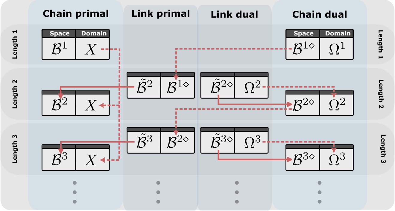
We start with an RKBS pair with domains and respectively, and kernel , which we call the initial RKBS pair. To construct a chain RKBS pair, the RKBS pair , with domains and , we need to first introduce a different pair of RKBS, which we call a link RKBS pair, which we denote with a tilde.
Let , be an RKBS pair with domains and , and has a kernel . Note that contains functions of , which itself are functions of . The kernels reproduce the functions in the following way
| (2.17) |
for all , and . Note that if contains only linear functions, the space is basically just and the rest of the construction becomes trivial. Therefore, in later sections, we choose such that it contains nonlinear functions, which is relevant when we apply this to neural networks. Also, for neural networks the set is chosen as , which makes the link spaces more symmetrical, but this is not necessary for the general construction.
By composing the kernels in a certain way, we create a new RKBS with domain . To be precise, we define using the quotient space of Theorem 3 with the feature map :
| (2.18) |
One way to view this construction is that the kernel , selects which functionals of become the evaluation functionals of . The feature map is well-defined, because is an element of , by definition of the adjoint pair of RKBS. This defines the linear map , which maps elements to functions of
| (2.19) |
We formally define the Banach space as the image of the map , which is a subspace of the vector space of functions with domain . The norm of is defined by the norm of the quotient space over the nullspace .
| (2.20) |
for all , and for any such that . The nullspace of is given by
| (2.21) |
We define the space as the subspace of which annihilates , i.e.
| (2.22) |
The subspace embedding is given by the identity map , and the norm as well as function evaluation on are inherited from .
| (2.23) |
for all and .
The pairing between and is also inherited
| (2.24) |
for all and some such that .
Now that we have defined the chain spaces and , we show that this construction indeed generates a new RKBS pair.
Theorem 7 (RKBS Consistency).
The spaces , form an RKBS pair with kernel for all .
Proof.
By Theorem 3, we immediately get that is an RKBS. Since is an RKBS and is equipped with the subspace norm, must also be an RKBS by Definition 2.
The pairing (2.24) is bounded, as
| (2.25) |
for all and all such that . Taking the infimum over all such , we get the required bound.
Next, to show that the pairing is non-degenerate: First, if such that for all , then for all and such that . From the definition of it follows that , and thus . Second, if such that for all , then for all . Hence, by the non-degeneracy of this pairing, we get that and as the embedding is injective, . Thus, we conclude that form a dual pair of Banach spaces.
Let . For the evaluation functional , we get for all that , as is a kernel. Hence and
| (2.26) |
for all and all such that .
Let . For the evaluation functional . Hence, and
| (2.27) |
for all .
Thus, we conclude that , form a pair of RKBS with kernel . ∎
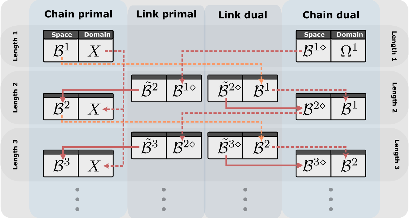
By defining new link RKBS pairs , for , we can build longer chain RKBS pairs for any length . Note that this procedure is not symmetric: still has domain , while has domain . This makes sense from a standpoint of neural networks as if we add layers, we get more weights, while the input space stays the same.
For Hilbert spaces, the construction takes the following simplified form. We start with an initial RKHS with domain and kernel , and a link RKHS with domain with kernel . The procedure above then leads to a chain RKHS with domain and kernel .
3 Chain RKBS for Deep Neural Networks
In the previous section, we showed that given a kernel, there exists a RKBS pair with that kernel, which we can use to build a chain RKBS. In this section, we will make this construction more concrete by choosing specific spaces such that it correspond to deep neural networks.
First, we restrict ourselves to integral chain RKBS, or integral cRKBS for short. Afterwards, we will choose the kernel such that it corresponds to an element-wise activation function and an affine combination, which is common in neural networks. We will show that for the ReLU activation function, our description is equivalent to the generalised Barron spaces of E and Wojtowytsch (2020).
3.1 Integral cRKBS
Integral RKBSs are RKBSs where the functions with domain are described by integrating the kernel with respect to some measure over (or vice versa).
To be precise, we start with completely regular Hausdorff sets and and a bounded, measurable function , where measurable is always understood to be Borel measurable. We define to be the Banach spaces of Radon measures of , respectively with the total variation norm, i.e. regular signed Borel measures with finite total variation. The Dirac or point measures are denoted by , for and respectively. We then define the integral RKBS pair as follows:
Definition 8.
Let be sets with a completely regular Hausdorff topology, and let be bounded and measurable. An integral RKBS pair is defined as follows: For all there exists a such that
| (3.1) |
for all , for all there exists a such that
| (3.2) |
for all , and the pairing between and is given by
| (3.3) |
for some such that and .
Note that is always defined to have a ’1-norm’ and an ’-norm’. In a previous paper (Spek et al., 2023), we have already shown that satisfy all the conditions to be an RKBS pair, if and the kernel is continuous. The proof for this more general setting is analogous, so we will only give a short sketch of the proof.
Theorem 9.
The spaces , with the pairing of Definition 8 form a pair of RKBS with kernel .
Proof.
Now, to expand our initial RKBS pair to an integral cRKBS pair, we can use the procedure of the Section 2.2. We only need to choose completely regular Hausdorff and bounded, measurable kernels for some . We can then define the link RKBS pairs to be the integral RKBS pair corresponding to , see Definition 8. Note that here elements of are functions of , i.e. for each there exists a
| (3.4) |
for all .
From these link RKBS pairs , we can use the construction of Section 2.2 to formulate a cRKBS pair with domains . These spaces are again integral RKBS with
Theorem 10 (Integral Consistency).
Let , . If is an integral RKBS pair with domains and kernel , and are integral RKBS pairs with domains with kernel for all , then the cRKBS pair with domains is an integral RKBS pair with kernel .
Proof.
We will prove that are integral RKBS pairs by induction on and then the form of the kernel follows directly from Theorem 7. The base case of is true by definition.
Suppose are an integral cRKBS pair, for some . Then by Theorem 7 form an RKBS pair with domains and kernel . As are bounded, so is , and by Theorem 6 this kernel is unique. What remains to be shown is that satisfy the extra requirements to be of integral RKBS, as in Definition 8.
To check (3.1), define
| (3.5) |
for all and . By construction of ,
| (3.6) |
Hence, functions in satisfy (3.1).
To check (3.2), define
| (3.7) |
for all , , and . From the inclusion relation of into it follows that there exists a for all such that , but need to show that there exists a such that . We use the definition of and the map to explicitly construct a for each .
If , then
| (3.8) |
for all . Hence, if , then
| (3.9) |
for all and some such that . Thus, any can be written as
| (3.10) |
for some with restriction to given by . Since , the push-forward of the measure from to along , is an element of , the functions in satisfy (3.2).
This shows that integral cRKBS are indeed standard integral RKBS with more complicated kernels. In the next section, we will choose particular kernels which correspond to neural networks.
3.2 Neural cRKBS
Deep neural networks, like multi-layer perceptrons, are characterised by alternating affine transformations and elementwise nonlinearities. The natural infinite width extension can be described by an integral cRKBS with a certain kernel, which is composed of alternating affine transformations and elementwise nonlinearities. We call these spaces neural cRKBS. In this section, we will describe how neural cRKBS are constructed and show that the neural tree spaces defined in E and Wojtowytsch (2020) are a specific instance of such a neural cRKBS.
We start with the neural network case with a single layer. First, we need to define a vector space structure on and , so we can meaningfully define the notion of a linear layer. We take , where are a dual pair of normed vector spaces. Note that in most applications, these spaces are , where is the dimension of the input data. The is added to represent the bias. To be a neural RKBS, the kernel has to take the form
| (3.12) |
where , is some (nonlinear) function, called the activation function, and , a weighting function such that is bounded.
A well-known example of a neural RKBS is the Barron space, although it is more often written in the form where is moved into the total variation norm of the representing measures. For a detailed investigation of these spaces, see (Spek et al., 2023).
Definition 11.
Let , where are a dual pair of normed vector spaces. Let and be measurable and positive, and such that is bounded, where for all and .
If are an integral RKBS pair with kernel , then are a neural RKBS pair.
In this definition, the purpose of the weighting function is to ensure that the kernel is bounded even when and are not. This is a technical complication to accommodate certain commonly used activation functions. For example, if is a neural RKBS with domain , some bounded subset of , and parameter space , activation function and weighting function . The activation function is an unbounded Lipschitz continuous function with Lipschitz constant 1, and the weighting function ensures that
| (3.13) |
for all . It is also possible to avoid using the weighting function by changing the definition of the integral RKBS to only consider measures such that (3.1) is integrable for all . However, this makes the analysis below much more complicated, so we opt to use a weighting function instead.
To extend these ideas to chain RKBSs, we need a similar linear structure for the domains of the link spaces . We can do this by taking , where we leverage the natural linear structure given by the pairing. Note that the -relation is cross-linked: contains functions of and functions of . These link spaces are neural RKBS when their kernel is of the form
| (3.14) |
for all , , activation function , and weighting function .
This leads to the formal definition of a neural cRKBS: a chain RKBS where the initial and link RKBS are neural RKBS. For a graphical description of the neural RKBS chain process, see Figure 3.
Definition 12.
An integral cRKBS pair with domains and kernel are called a neural cRKBS pair if the initial RKBS pair is a neural RKBS pair with domains , with activation function and with weighting function , and if the link RKBS pairs are neural RKBS pairs with domains , with activation functions and with weighting functions for all .
Note that by construction these neural cRKBSs are ’regular’ RKBSs: They have a proper norm, are complete vector spaces and have a kernel. This abstract definition implies that the functions of these RKBS have a particular recursive form:
| (3.15) |
where . To paraphrase this equation, a neural cRKBS of length has functions that are linear combinations of functions of a neural cRKBS of length with applied to them. This form is due to the particular structure of the kernel .
Theorem 13.
If be a neural cRKBS pair with given , activation functions and weighting functions for , then the kernel is given by
| (3.16) |
for all and .
Proof.
As is an element of an integral RKBS, there exists a measure such that . This allows us to expand the kernel in the following way
| (3.18) |
Here we now more clearly see the neural network structure of the neural cRKBS: The kernel of layer is the composition of an activation function , an affine transformation with weights and bias , and the kernel of the previous layer . The non-linearity is elementwise because acts on the function evaluated at , which is the natural extension of the concept of elementwise to RKBSs.
The neural cRKBS with contains all the multi-layer perceptrons of length L with arbitrary widths at each layer with given activation functions. The key idea here is that we can choose as a linear combination of Dirac measures. When are chosen smaller, can be restricted to only networks where weights are bounded, or to represent convolutional layers, or other linear layers that respect some symmetry for example.
Theorem 14.
Let . Let be a neural cRKBS pair with , for , and activation functions and weighting functions , for . Furthermore, let and weight matrices for and bias vectors for and row vector . If the deep neural network is given by
| (3.19) |
for all in which are the elementwise extensions of for , then and
| (3.20) |
where
| (3.21) |
with the th row of .
Proof.
We will prove that by induction on . First, the case where . Let be a shallow neural network
| (3.22) |
We choose
| (3.23) |
where are Dirac measures and the th row of . We have that , as .
| (3.24) |
Suppose is a neural network of length . Then we can write as the last layer acting on a collection of , for .
| (3.25) |
By the induction hypothesis for all , so we choose
| (3.26) |
We have that , as .
| (3.27) |
Furthermore, the definition of the norm of implies that
| (3.28) |
∎
For most activation functions we can set to be constant, so the norm of is just the 1-norm of the weights of the last linear layer.
3.3 Relation to other spaces
In this section, we will discuss how the neural cRKBS relates to other function spaces for deep networks, like generalised Barron spaces and hierarchical spaces. We will not consider bottlenecked spaces, as this approach based on function composition is incompatible with kernel composition.
The neural tree spaces of E and Wojtowytsch (2020) are a special case of a neural cRKBS . With the choices , some fixed compact set , , , the unit ball in without biases, , the rectified linear unit and , because is continuous and both and are bounded, we exactly retrieve the definition of the space of Section 3.1 of E and Wojtowytsch (2020). This paper however does not have a dual framework, so the has no analogue.
The authors show that for this space there are direct and inverse approximation theorems and that the norm in this space for deep networks is equivalent to a path norm
| (3.29) |
This result is to be expected as the ReLU functions are homogeneous. Therefore, the sizes of the inner weights can be moved to the last layer weight and keep the inner weights in a unit ball. One can reformulate this space with a full domain by introducing a weighting function .
The original definition of the does not include a bias. In general, if the constant function is included in , the term with and can be rewritten as . A push-forward argument shows that this leads to an isomorphism between the primals of the pairs with and without biases. It depends on the weighting function whether this isomorphism is isometric. Removing the bias implies a different , so the functions have a different domain. However, each of these can be thought of as a restriction to the domain without a bias.
Lemma 15.
Let be a neural cRKBS pair with domains . Consider the neural link RKBS pairs and with domains and respectively, activation functions as well as weighting functions satisfying . Moreover, let be the neural cRKBS constructed from by linking for . If and , then and are isomorphic, and the restriction of to is .
Proof.
The embedding of into is immediate.
For the converse, let . There exists a measure so that
where with
| (3.30) |
and
| (3.31) |
Taking the infimum over shows the embedding of into .
Denote with the restriction map, i.e.
| (3.32) |
for and . This map is linear with
| (3.33) |
and ∎
Now we can show that the neural tree space is equivalent to neural cRKBS with .
Theorem 16.
Let , compact, and denote with the neural tree spaces. If , and , then is a neural cRKBS with isometrically isomorphic to for all .
Proof.
This is a proof by induction, with the base case following from Spek et al. (2023). Moreover, , which follows by choosing the measure .
For the induction step, assume that with and isometrically isomorphic to . Define
| (3.34) |
To show the isometric isomorphism between and , we will show that both are isometrically isomorphic to . The isometric isomorphism between and follows from the homogeneity of ReLU. For the isometric isomorphism between and , observe that the choice of and the assumption on together imply that
| (3.35) |
It follows that the versions of with and without bias are isometrically isomorphic. This combined with the isometric isomorphism between and shows the isometric isomorphism between and . What remains to show is that with . This follows by choosing the measure . ∎
Neural Hilbert Ladders are defined by means of sequences of Hilbert spaces. These sequences have a similar pattern as the construction of the cRKBSs. In fact, the considered Hilbert spaces are neural cRKHS.
A cRKHS is constructed using a RKHS over and a RKHS over . Following the procedure outlined for cRKBS in section 2.2, the feature is given by
| (3.36) |
in which is the kernel of and is the kernel of . The resulting kernel is
| (3.37) |
the kernel of the RKHS , in which the Hilbert space is a feature space for .
If the cRKHS is of neural-type with for some probability measure with bounded second moment and the activation function is Lipschitz, then the kernel satisfies
| (3.38) |
This agrees with the structure of in (1.5). Repeating this process shows that the Hilbert spaces in the infimum of (1.6) are indeed neural cRKHSs. However, the space constructed by taking the infimum over these cRKHSs, loses the RKHS structure, in contrast to the neural cRKBS.
4 Representer Theorem: kernel chains enable weight sharing
So far, we have shown that neural cRKBSs are a natural infinite width limit of deep neural networks, which gives insight into their general properties. In most applications, however, we have only a finite amount of data points. In this case, all functions in such neural cRKBSs can be represented by (finite) deep neural networks.
Given data points, an application of the representer theorem to (3.15), reduces the integral of to a linear combination of functions . Repeating this procedure would lead to an exponential amount of nodes in . Here the kernel and duality structure of our spaces can significantly improve this estimate, as a set of at most evaluation functionals form a basis of an RKBS pair, when we have only finite data points. Decomposing the using a basis, allows them to share weights and leads to a neural network with at most hidden nodes at each layer.
Lemma 17.
Let be a pair of RKBS with domains , and kernel . If is finite, then and there exists elements such that forms a basis of , where .
Proof.
Let have finite cardinality. Choose such that the set is a maximally linear independent subset of .
We can pick , for , such that the matrix with the elements has full rank, because it has linear independent rows for . Thus, the columns of this matrix , for , must also be linearly independent.
It remains to show that spans . Let , and take . Define , then for all . With the set chosen to be maximally linearly independent for all , the definition of a Banach space of functions implies that is the zero vector and .
Since are a dual pair of Banach Spaces, they embed in each other duals:
| (4.1) |
We have shown previously that has dimension which together with the embeddings implies that
| (4.2) |
Thus, and have the same dimension, . The set is linear independent and of size , hence it also must span and the full set does as well. ∎
Using this Lemma, we can prove the main theorem of this section, which can be thought of as the converse of Theorem 14: When is finite, all functions are deep networks. In this case, they even have at most hidden neurons at each layer and the inner weights and biases are fixed for a given and functions .
Theorem 18.
Let . Let be a neural cRKBS pair with , activation functions and weighting functions , where .
If is finite and , then there exists weight matrices , for , and bias vectors for such that for all , there exists a row vector such that for all
| (4.3) | ||||
| (4.4) |
where are the elementwise extensions of , for , and where
| (4.5) |
Proof.
Let have finite cardinality and let . Then by Lemma 17, there exists for , such that are a basis of . We set . Then by the induction hypothesis on there exists weight matrices , for , and bias vectors for , and row vectors for such that
| (4.6) |
We choose the weight matrix as the matrix with rows for .
Corollary 19 (Deep representer theorem for neural cRKBS).
Let . Let be a neural cRKBS pair with , activation functions and weighting functions , where .
Let and consider data points , for . If is proper convex, coercive, lower semi-continuous with respect to the Euclidean norm, and dependent on , then the optimisation problem
| (4.11) |
admits solutions of the form
| (4.12) |
for . Here, the parameters are the weight matrices , for and the bias vectors for and the row vector , and the are the elementwise extensions of , for .
Proof.
Remark.
By construction, the neural cRKBS have only real-valued functions, and so can only contain neural networks with a single output dimension. However, when we have vector-valued output , such a neural network can be thought of as a vector of . As these scalar-valued deep networks share weights, we get a similar result as above but with .
When we have finite data, the norm on the dual space for an integral pair of RKBS gives a complexity measure on . Note that by replacing the in the theorem with Gaussian variables, we get the Gaussian complexity instead of the Rademacher complexity.
Theorem 20.
Let be an integral pair of RKBS with domains , and kernel . Let be finite, and let be i.i.d. Rademacher random variables. Define the -valued random variable as follows
| (4.13) |
The empirical Rademacher complexity of the unit ball of for is given by the expectation of the norm of
| (4.14) |
Proof.
As for , . By Lemma 17 the convex hull of the set gives the unit ball of , so we may equivalently look at the Rademacher complexity of this set.
∎
5 Discussion
In this paper, we have shown that by composing kernels of RKBS pairs, we can form a natural function space for deep neural networks. These neural cRKBSs contain all deep neural networks. For finite data, the functions in these spaces reduce to deep networks of a width of at most the size of the data.
Such neural cRKBS have a regular structure from an analysis standpoint: They have norms, are complete, and have a well-described duality structure between weights and data: On one side, contains functions of the data and on the other side contains functions over which represents the set of all the weights, except for the final layer. Here, we also see, why the RKBS framework is more suitable to describe deep neural networks than an RKHS framework. In a chain RKBS the stays the same, while the can adapt: for a deeper neural network, the input size stays the same, but we get more weights. For a chain RKHS, the symmetry requires that stays fixed, equal to .
In this neural cRKBS space, the resulting optimisation problem (4.11) actually becomes convex. However, if we reduce to finite deep neural networks using the representer theorem, finding the inner weights is a non-convex problem. The trade-off between finite dimensionality and convexity is a common feature in RKBSs, in comparison to RKHSs, where the representer theorem gives constructive solutions. This corresponds to deep neural networks, where gradient descent is used to overcome the non-convexity.
In some sense, the neural cRKBS gives us deep neural networks where instead of finding a finite set of weights, we take any (Radon) distribution of weights. The final linear layer brings it back together by choosing a linear combination of all the possibilities, which is a convex problem. In previous work, (Spek et al., 2023, Corollary 13), we have shown that integral RKBSs are a union of RKHSs each corresponding to a choice of inner weights, showing that indeed these RKBSs form the set of all possible choices.
The construction using kernel chains provides a concrete description of the dual space . Its norm is a measure of the expressivity of via the complexity of its unit ball. The optimisation problem (4.11) for the neural cRKBS also allows for a dual problem (Spek et al., 2023, Theorem 18 and 20). However, this again leads to a non-convex problem, where we need to find the inner weights that form the basis of .
6 Summary and outlook
In this final section, we summarise our work at a higher level and highlight research areas where our theory could have a potential impact in the future.
In this work, we addressed the fundamental question of identifying an appropriate function space for deep networks. At first glance, one might think that function compositions are a natural concept for networks in depth. However, at second glance, they have the unique limitation in depth that extra hidden bottleneck layers (with potentially different widths) appear, which prevent desirable reproducing properties in the function space. To overcome this key limitation, we introduced the reproducing kernel chain framework (cRKBS). By composing kernels rather than functions, we could naturally preserve desired properties from single-layer reproducing kernel Banach spaces through depth.
This paradigm shift via kernel representations and duality has the potential to offer new perspectives and solutions for deep learning theory and practice in the future. In the following paragraphs, we highlight four of such potential impact areas.
In geometric deep learning (Bronstein et al., 2021), weight-sharing in widths has offered fascinating insights over the past years from translational-invariant CNNs via group-invariant layers to Clifford algebra layers in GNNs. However, especially given deep networks representing solutions via neural ODEs, neural PDEs, or more generally via operator learning (Boullé and Townsend, 2023), a promising prospect would be to study geometric and sparsity properties of cRKBS as weight-sharing in-depth.
In the context of random feature models and optimisation, the role of sampling weights of deep neural networks (Bolager et al., 2023) has proven to be a successful concept for the construction of trained networks orders of magnitude faster than with conventional training schemes. Because of the primal-dual nature of the chains and links in our kernel chaining framework, our findings could offer new insights into deep weight sampling as well as for sparsity promoting optimization in deep architecture search (Heeringa et al., 2024a, 2023).
An important prospect of this work also lies in generalisation theory (Zhang et al., 2021). Building upon existing work on Rademacher complexity for function classes, it could be interesting to explore the role of reproducing kernel chains and bounds related to the VC dimension. For this, the finite-data to finite-weight relationship in our reproducing kernel chaining framework could be of particular interest.
Despite the recent big success of graph neural networks and transformers for imaging and large language models, a deeper understanding of the attention mechanism in depth would be important. Whereas for basic graph neural networks, the connection to Barron spaces is investigated, a more detailed comparison of our work with this work (Wright and Gonzalez, 2021) could be promising to explore further.
Those four impact areas alone are already very promising. However, throughout this work, it was also an interesting observation that the reproducing kernel chaining concept is more general than deep neural networks. It is intriguing to think in the future about relaxing the assumptions on deep neural networks and what this could offer in practice.
References
- Aronszajn [1950] N. Aronszajn. Theory of reproducing kernels. Transactions of the American Mathematical Society, 68(3):337–404, 1950. ISSN 0002-9947, 1088-6850. doi: 10.1090/S0002-9947-1950-0051437-7. URL https://www.ams.org/tran/1950-068-03/S0002-9947-1950-0051437-7/.
- Bach [2017] Francis Bach. Breaking the Curse of Dimensionality with Convex Neural Networks. Journal of Machine Learning Research, 18(19):1–53, 2017. URL http://jmlr.org/papers/v18/14-546.html.
- Bartolucci et al. [2023] Francesca Bartolucci, Ernesto De Vito, Lorenzo Rosasco, and Stefano Vigogna. Understanding neural networks with reproducing kernel Banach spaces. Applied and Computational Harmonic Analysis, 62:194–236, January 2023. ISSN 1063-5203. doi: 10.1016/j.acha.2022.08.006. URL https://www.sciencedirect.com/science/article/pii/S1063520322000768.
- Bartolucci et al. [2024a] Francesca Bartolucci, Marcello Carioni, José A. Iglesias, Yury Korolev, Emanuele Naldi, and Stefano Vigogna. A Lipschitz spaces view of infinitely wide shallow neural networks, October 2024a. URL http://arxiv.org/abs/2410.14591. arXiv:2410.14591.
- Bartolucci et al. [2024b] Francesca Bartolucci, Ernesto De Vito, Lorenzo Rosasco, and Stefano Vigogna. Neural reproducing kernel Banach spaces and representer theorems for deep networks, March 2024b. URL http://arxiv.org/abs/2403.08750. arXiv:2403.08750 [cs, math, stat] version: 1.
- Bolager et al. [2023] Erik L. Bolager, Iryna Burak, Chinmay Datar, Qing Sun, and Felix Dietrich. Sampling weights of deep neural networks. Advances in Neural Information Processing Systems, 36:63075–63116, December 2023. URL https://proceedings.neurips.cc/paper_files/paper/2023/hash/c7201deff8d507a8fe2e86d34094e154-Abstract-Conference.html.
- Boullé and Townsend [2023] Nicolas Boullé and Alex Townsend. A Mathematical Guide to Operator Learning, December 2023. URL http://arxiv.org/abs/2312.14688. arXiv:2312.14688 [math].
- Bredies and Carioni [2019] Kristian Bredies and Marcello Carioni. Sparsity of solutions for variational inverse problems with finite-dimensional data. Calculus of Variations and Partial Differential Equations, 59(1):14, December 2019. ISSN 1432-0835. doi: 10.1007/s00526-019-1658-1. URL https://doi.org/10.1007/s00526-019-1658-1.
- Bronstein et al. [2021] Michael M. Bronstein, Joan Bruna, Taco Cohen, and Petar Veličković. Geometric Deep Learning: Grids, Groups, Graphs, Geodesics, and Gauges, May 2021. URL http://arxiv.org/abs/2104.13478. arXiv:2104.13478 [cs].
- Caragea et al. [2020] Andrei Caragea, Philipp Petersen, and Felix Voigtlaender. Neural network approximation and estimation of classifiers with classification boundary in a Barron class. arXiv:2011.09363 [math, stat], November 2020. URL http://arxiv.org/abs/2011.09363. arXiv: 2011.09363.
- Chen [2024] Zhengdao Chen. Neural Hilbert Ladders: Multi-Layer Neural Networks in Function Space. Journal of Machine Learning Research, 25(109):1–65, 2024. ISSN 1533-7928. URL http://jmlr.org/papers/v25/23-1225.html.
- Chizat et al. [2019] Lénaïc Chizat, Edouard Oyallon, and Francis Bach. On Lazy Training in Differentiable Programming. In Advances in Neural Information Processing Systems, volume 32. Curran Associates, Inc., 2019. URL https://papers.neurips.cc/paper_files/paper/2019/hash/ae614c557843b1df326cb29c57225459-Abstract.html.
- E and Wojtowytsch [2020] Weinan E and Stephan Wojtowytsch. On the Banach spaces associated with multi-layer ReLU networks: Function representation, approximation theory and gradient descent dynamics. arXiv:2007.15623 [cs, math, stat], July 2020. URL http://arxiv.org/abs/2007.15623. arXiv: 2007.15623.
- E. and Wojtowytsch [2022] Weinan E. and Stephan Wojtowytsch. Representation formulas and pointwise properties for Barron functions. Calculus of Variations and Partial Differential Equations, 61(2):46, February 2022. ISSN 1432-0835. doi: 10.1007/s00526-021-02156-6. URL https://doi.org/10.1007/s00526-021-02156-6.
- E et al. [2020] Weinan E, Chao Ma, Stephan Wojtowytsch, and Lei Wu. Towards a Mathematical Understanding of Neural Network-Based Machine Learning: what we know and what we don’t. arXiv:2009.10713 [cs, math, stat], December 2020. URL http://arxiv.org/abs/2009.10713. arXiv: 2009.10713.
- E et al. [2022] Weinan E, Chao Ma, and Lei Wu. The Barron Space and the Flow-Induced Function Spaces for Neural Network Models. Constructive Approximation, 55(1):369–406, February 2022. ISSN 1432-0940. doi: 10.1007/s00365-021-09549-y. URL https://doi.org/10.1007/s00365-021-09549-y.
- Hanin [2023] Boris Hanin. Random neural networks in the infinite width limit as Gaussian processes. The Annals of Applied Probability, 33(6A):4798–4819, December 2023. ISSN 1050-5164, 2168-8737. doi: 10.1214/23-AAP1933. URL https://projecteuclid.org/journals/annals-of-applied-probability/volume-33/issue-6A/Random-neural-networks-in-the-infinite-width-limit-as-Gaussian/10.1214/23-AAP1933.full. Publisher: Institute of Mathematical Statistics.
- He et al. [2024] Fan He, Mingzhen He, Lei Shi, Xiaolin Huang, and Johan A. K. Suykens. Learning Analysis of Kernel Ridgeless Regression with Asymmetric Kernel Learning, June 2024. URL http://arxiv.org/abs/2406.01435. arXiv:2406.01435.
- He et al. [2022] Mingzhen He, Fan He, Lei Shi, Xiaolin Huang, and Johan A. K. Suykens. Learning with Asymmetric Kernels: Least Squares and Feature Interpretation, February 2022. URL http://arxiv.org/abs/2202.01397. arXiv:2202.01397.
- Heeringa et al. [2023] Tjeerd Jan Heeringa, Tim Roith, Christoph Brune, and Martin Burger. Learning a Sparse Representation of Barron Functions with the Inverse Scale Space Flow, December 2023. URL http://arxiv.org/abs/2312.02671. arXiv:2312.02671 [cs, math, stat].
- Heeringa et al. [2024a] Tjeerd Jan Heeringa, Christoph Brune, and Mengwu Guo. Sparsifying dimensionality reduction of PDE solution data with Bregman learning, June 2024a. URL http://arxiv.org/abs/2406.12672. arXiv:2406.12672 [cs, math, stat].
- Heeringa et al. [2024b] Tjeerd Jan Heeringa, Len Spek, Felix L. Schwenninger, and Christoph Brune. Embeddings between Barron spaces with higher-order activation functions. Applied and Computational Harmonic Analysis, 73:101691, November 2024b. ISSN 1063-5203. doi: 10.1016/j.acha.2024.101691. URL https://www.sciencedirect.com/science/article/pii/S106352032400068X.
- Huang et al. [2023] Wentao Huang, Houbao Lu, and Haizhang Zhang. Hierarchical Kernels in Deep Kernel Learning. Journal of Machine Learning Research, 24(391):1–30, 2023. ISSN 1533-7928. URL http://jmlr.org/papers/v24/23-0538.html.
- Jacot et al. [2020] Arthur Jacot, Franck Gabriel, and Clément Hongler. Neural Tangent Kernel: Convergence and Generalization in Neural Networks, February 2020. URL http://arxiv.org/abs/1806.07572. arXiv:1806.07572 [cs, math, stat].
- Li et al. [2020] Zhong Li, Chao Ma, and Lei Wu. Complexity Measures for Neural Networks with General Activation Functions Using Path-based Norms. arXiv:2009.06132 [cs, stat], September 2020. URL http://arxiv.org/abs/2009.06132. arXiv: 2009.06132.
- Lin et al. [2022] Rong Rong Lin, Hai Zhang Zhang, and Jun Zhang. On Reproducing Kernel Banach Spaces: Generic Definitions and Unified Framework of Constructions. Acta Mathematica Sinica, English Series, 38(8):1459–1483, August 2022. ISSN 1439-7617. doi: 10.1007/s10114-022-1397-7. URL https://doi.org/10.1007/s10114-022-1397-7.
- Liu et al. [2021] Fanghui Liu, Lei Shi, Xiaolin Huang, Jie Yang, and Johan A. K. Suykens. Generalization Properties of hyper-RKHS and its Applications. Journal of Machine Learning Research, 22(140):1–38, 2021. ISSN 1533-7928. URL http://jmlr.org/papers/v22/19-482.html.
- Neumayer and Unser [2023] Sebastian Neumayer and Michael Unser. Explicit representations for Banach subspaces of Lizorkin distributions. Analysis And Applications, July 2023. ISSN 0219-5305. doi: 10.1142/S0219530523500148. URL https://infoscience.epfl.ch/handle/20.500.14299/199724.
- Parhi and Nowak [2021] Rahul Parhi and Robert D. Nowak. Banach Space Representer Theorems for Neural Networks and Ridge Splines. Journal of Machine Learning Research, 22(43):1–40, 2021. URL http://jmlr.org/papers/v22/20-583.html.
- Parhi and Nowak [2022] Rahul Parhi and Robert D. Nowak. What Kinds of Functions Do Deep Neural Networks Learn? Insights from Variational Spline Theory. SIAM Journal on Mathematics of Data Science, 4(2):464–489, June 2022. doi: 10.1137/21M1418642. URL https://epubs.siam.org/doi/abs/10.1137/21M1418642. Publisher: Society for Industrial and Applied Mathematics.
- Rahimi and Recht [2007] Ali Rahimi and Benjamin Recht. Random Features for Large-Scale Kernel Machines. In Advances in Neural Information Processing Systems, volume 20. Curran Associates, Inc., 2007. URL https://papers.nips.cc/paper_files/paper/2007/hash/013a006f03dbc5392effeb8f18fda755-Abstract.html.
- Shenouda et al. [2024] Joseph Shenouda, Rahul Parhi, Kangwook Lee, and Robert D. Nowak. Variation Spaces for Multi-Output Neural Networks: Insights on Multi-Task Learning and Network Compression, July 2024. URL http://arxiv.org/abs/2305.16534. arXiv:2305.16534.
- Spek et al. [2023] Len Spek, Tjeerd Jan Heeringa, Felix Schwenninger, and Christoph Brune. Duality for Neural Networks through Reproducing Kernel Banach Spaces, March 2023. URL http://arxiv.org/abs/2211.05020. arXiv:2211.05020 [cs, math].
- Woodworth et al. [2020] Blake Woodworth, Suriya Gunasekar, Jason D. Lee, Edward Moroshko, Pedro Savarese, Itay Golan, Daniel Soudry, and Nathan Srebro. Kernel and Rich Regimes in Overparametrized Models. In Proceedings of Thirty Third Conference on Learning Theory, pages 3635–3673. PMLR, July 2020. URL https://proceedings.mlr.press/v125/woodworth20a.html. ISSN: 2640-3498.
- Wright and Gonzalez [2021] Matthew A. Wright and Joseph E. Gonzalez. Transformers are Deep Infinite-Dimensional Non-Mercer Binary Kernel Machines, June 2021. URL http://arxiv.org/abs/2106.01506. arXiv:2106.01506 [cs].
- Zhang et al. [2021] Chiyuan Zhang, Samy Bengio, Moritz Hardt, Benjamin Recht, and Oriol Vinyals. Understanding deep learning (still) requires rethinking generalization. Communications of the ACM, 64(3):107–115, March 2021. ISSN 0001-0782, 1557-7317. doi: 10.1145/3446776. URL https://dl.acm.org/doi/10.1145/3446776.
- Zhang et al. [2009] Haizhang Zhang, Yuesheng Xu, and Jun Zhang. Reproducing kernel Banach spaces for machine learning. In 2009 International Joint Conference on Neural Networks, pages 3520–3527, Atlanta, Ga, USA, June 2009. IEEE. ISBN 978-1-4244-3548-7. doi: 10.1109/IJCNN.2009.5179093. URL http://ieeexplore.ieee.org/document/5179093/.