Extreme-temperature single-particle heat engine

Abstract

Carnot famously showed that engine operation is chiefly characterised by the magnitude of the temperature ratio $T_{\mathrm{h}}/T_{\mathrm{c}}$ between its hot and cold reservoirs. While temperature ratios ranging between $1.3-2.8$ and $2-10$ are common in macroscopic commercial engines and engines operating in the microscopic regime, respectively, the quest is to test thermodynamics at its extremes. Here we present the hottest engine on earth, with temperature ratios as high as $110$. We achieve this by realising an underdamped single-particle engine using a charged microparticle that is electrically levitated under vacuum conditions. Noisy electric fields are used to synthesise reservoir temperatures in excess of $10^{7}$ K. As a result, giant fluctuations show up in all thermodynamic quantities of the engine, such as heat exchange and efficiency. Moreover, we find that the particle experiences an effective position dependent temperature, which gives rise to dynamics that drastically deviates from that of standard Brownian motion. We develop a theoretical model accounting for the effects of this multiplicative noise and find excellent agreement with the measured dynamics. The high level of control over the presented experimental platform opens the door to emulate the stochastic dynamics of cellular and biological processes, and provides thermodynamic insight required for the development of nanotechnologies.

Introduction. The thermodynamic behaviour of microscopic systems is full of surprises; engines can run backwards for a short time [1], diffusion can be directed [2] and the thermal environment remembers where you were [3]. Accurate models of microscale thermodynamics are critical for understanding the transport in cell-biology [4] and for the design of micromachines. When the fluctuation in the exchange of energy between a system and its environment become comparable to the energy of the system itself, we must move beyond only considering averaged behaviour, and understand the statistics of individual stochastic trajectories [5, 6].

Single microparticles confined in harmonic potentials, typically created by optical tweezers [7], are recognized as the paradigmatic system in which to study stochastic thermodynamics [5, 8, 9], since their average motional energy is comparable in scale to the fluctuating exchange of energy with their environment. It is possible to track the motion of confined particles with high resolution, such that small fluctuations can be measured, and to utilize an impressively well-stocked toolbox of control techniques [7, 10, 11, 12]. The system has enabled seminal studies of information thermodynamics [13, 14] and elucidated microscopic thermal dynamics [15, 16, 3, 17]. Previous work has shown that by levitating single microparticles in a gas of controllable pressure one can tune the rate at which they exchange energy with their environment. Tuning the system-bath coupling has allowed observation of ballistic Brownian motion [18], equilibration at the single-trajectory level [19, 20], non-equilibrium energetics [21, 22, 23] and the transition from under- to over-damped bistability [24, 25, 23].

Figure 1: Schematic of the single particle engine. A charged silica microparticle is levitated within a linear Paul trap under vacuum conditions. Coaxial endcap control electrodes, separated by 1.6 mm, provide harmonic confinement along the $z$-axis, with a frequency that can be varied by changing the voltages $U_{0}$ applied to both electrodes. An additional fluctuating voltage with white-noise statistics $U_{T}$ applied to one control electrode generates a spatially varying synthetic heat bath (red), with temperatures in excess of $10^{7}$ K. To the right is shown an image of the microparticle at $14,000$ K (above) and $5,100,000$ K (below), illustrating how at high temperature the particle samples a wide region of the spatially varying heat bath.

In this work, we study the underdamped thermodynamics of a single microparticle exposed to an unprecedented scale of thermal fluctuation, characterized by an effective temperature of over 10,000,000 K and by the exchange of many hundred $k_{\mathrm{B}}T$ of heat with its environment at temperature $T$. We run a single particle heat engine by levitating a charged microparticle in a Paul trap under vacuum conditions, see Fig. 1, and synthesize high-temperature environments through the use of noisy electric fields [26]. The deep electrical potential $>10^{9}\,$K, as compared to more commonly used optical potentials with a depth $<10^{5}\,$K [11], allows us to achieve temperatures far in excess of previous single-particle engines [26, 27, 28]. Operating in the underdamped thermodynamic regime [29, 30, 31] enhances thermodynamic fluctuations as compared to experiments in liquid [1, 26]. Like many biological micro-systems, our engine experiences coordinate-dependent diffusion [32, 33, 34, 35], and we present accurate models to describe its behaviour. We study the heat, power and efficiency statistics of our system. We achieve average efficiencies of approximately 10% and remarkably measure single-cycle efficiency fluctuations far in excess of 100% [36, 37], a bold illustration of the surprising nature of thermodynamics at the microscale.

Experimental set-up. Our engine is realised by levitating a 4.82 $\mu$m diameter spherical silica particle with a charge-to-mass ratio of $q/m=(-0.355\pm 0.008)$ C/kg, corresponding to a negative charge in excess of $10^{4}\,e$. Levitation is achieved electrically with a linear Paul trap formed by four cylinders arranged on the corners of a square, and two additional co-axial cylindrical endcap electrodes separated by 1.6 mm positioned either side of the particle, see Fig. 1. The levitated particle moves as a 3D harmonic oscillator, where the three centre-of-mass modes of oscillation are independent, even at the highest bath temperatures we study.

By adjusting the voltage $U_{0}$ applied to both endcap electrodes, the trap frequency along the $z$-direction is changed cyclically between $f_{1}=(341.4\pm 0.1)\,$Hz and $f_{2}=(316.6\pm 0.1)\,$Hz. This is equivalent to changing the volume in a macroscopic engine cycle [5]. Damping is caused by the particle colliding with the room temperature gas at the operating pressure of $(2.3\pm 0.4)\crossproduct\rm{10}^{-3}\,$mbar, resulting in a momentum damping rate of $\gamma_{g}=(0.8\pm 0.1)\,$Hz. This puts our engine operation deep in the underdamped regime $f_{1,2}\gg\gamma_{g}$.

By applying white voltage noise $U_{T}$ to one of the endcap electrodes the effective centre-of-mass temperature of a single degree-of-freedom of the levitated particle can be changed [26]. Due to the potential depth of the Paul trap ($>10^{9}\,$K), we are able to increase the temperature of the particle in excess of $T_{\mathrm{h}}=10^{7}\,$K while remaining in the linear part of the Paul trap potential. We measure the centre-of-mass temperature of the particle via the power spectral density of its motion [38], see Supplementary Information for more details. At the highest temperatures, the standard deviation of the particle’s motion is in excess of $100\,\mu$m, as can be seen in the long-exposure images in Fig. 1. To track this motion while maintaining both high spatial and temporal resolution we use event-based imaging, which we have characterized elsewhere [39].

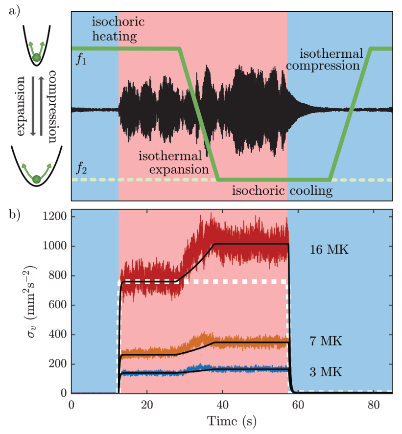
Figure 2: Engine cycle with position dependent diffusion. a) A single position trajectory (black trace) of a levitated microparticle undergoing a Stirling engine cycle (green) and b) averaged velocity variances $\sigma_{v}$ (coloured traces). In an isochoric heating step the temperature is changed from cold (blue shaded region) to hot (red shaded region), while the trap frequency is subsequently changed from $f_{1}$ to $f_{2}$ realizing isothermal expansion. The velocity variances $\sigma_{v}$ are at different hot-bath temperatures labeled in units of MK ($1\,$MK $=10^{6}\,$K). This experimental data is averaged over 1000 cycles with a time-bin of 1 ms. Solid black lines are obtained by numerically solving the dynamical equations of our model (21). The white dashed line is the predicted variance for standard Brownian motion, with the deviation from this prediction a clear indication of position dependent diffusion.

The electric field in the $z$-direction is not uniform (see Supplementary Information), hence the bath temperature generated by $U_{T}$ is not spatially uniform. Due to the amplitude of the trapped particle’s motion, it experiences a position-dependent temperature, which will prove to be critical in understanding the dynamics of our system.

We run a Stirling engine cycle as illustrated in Fig. 2 a). The particle is brought to equilibrium at a high temperature $T_{\mathrm{h}}$ through application of white voltage noise $U_{T}$. The Paul trap potential is quasistatically relaxed linearly over time (isothermal expansion) by evenly reducing the DC voltage $U_{0}$ on both endcap electrodes and the particle is again left to reach equilibrium. The white voltage noise $U_{T}$ is switched off, and the particle thermalizes with the surrounding gas and residual voltage noise, which determines the cold temperature $T_{\mathrm{c}}=34,000$ K. An isothermal compression step is achieved by evenly increasing the voltage on both endcap electrodes, completing the Stirling cycle. This cycle is repeated 700-1400 times at each value of $T_{\mathrm{h}}$.

Theoretical modeling. As we will see, a key feature of our electrically levitated particle engine is that fluctuations of thermodynamic quantities (around the mean values considered within macroscopic thermodynamics) can be enormous. Stochastic thermodynamics [5] provides the framework for the analysis of such dynamics. To model the dynamics of the particle, we set up the Fokker-Planck equation for the probability distribution ${\cal P}(z,v,t)$ of the particle having at time $t$ the position $z$ and velocity $v=\dot{z}$ in the $z$-direction. The voltage noise $U_{T}$ induces a stochastic electric field $E(z,t)=E_{0}(z)\,\xi(t)$, with magnitude $E_{0}(z)$ and $\xi(t)$ describing Gaussian white noise with zero mean, $\langle\xi(t)\rangle=0$, which is delta-correlated $\langle\xi(t)\xi(t^{\prime})\rangle=2\delta(t-t^{\prime})$, where $\langle\cdot\rangle$ is an average over an ensemble of stochastic trajectories. Note that the strength $E_{0}$ of the field experienced by the charged particle here depends on the particle’s position $z$.

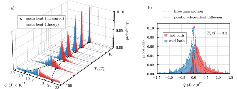
Figure 3: Stochastic engine heat distributions. a) Measured distribution of the heat $Q$ the levitated particle exchanges with the cold (blue) and hot (red) environment, respectively, as a function of temperature ratio $T_{\mathrm{h}}/T_{\mathrm{c}}$. The highly stochastic nature of the heat exchange is evident in the wide range of heat values. Distributions at the highest temperature ratio have been truncated for clarity. Negative (positive) heat values signify energy is transferred from (to) the particle’s motion to (from) the bath. The mean of these experimental distributions are marked with a black circle, with the theoretical prediction (Eq. 3) indicated by a dashed line. Values of heat exceed $10^{-18}$ J, equivalent to $>500\,k_{\mathrm{B}}T_{\mathrm{c}}$; much larger than previous single-particle heat engines ($<1\,k_{\mathrm{B}}T_{\mathrm{c}}$ [26, 28]) due to the extreme temperatures involved. b) A pair of heat distributions at a low temperature ratio of $T_{\mathrm{h}}/T_{\mathrm{c}}=3.3$. The stochastic nature of the energetic exchanges is particularly pronounced, as evidenced by the negative values of the particle’s heat absorption from the hot bath (red), i.e. the particle sometimes dumps heat into the hot bath, and vice versa cools the cold bath (blue, positive values). The experimental data is compared to predictions based on standard Brownian motion (dotted lines) and our model with position-dependent diffusion (solid lines, Eq. (3)), the latter showing better agreement with the data.

Adapting the form of a general multi-variate Langevin equation [40] to capture the experimental situation described above, we find

$$\partial_{t}{\cal P}(z,v,t)=$$ (1)

$$\left[-v\,\partial_{z}+\partial_{v}(\omega^{2}(z-z_{0})+\gamma_{g}v)+F^{2}(z)\,\partial_{v}^{2}\right]\!{\cal P}(z,v,t),$$

where $\omega=2\pi f$ and $z_{0}$ are the trap angular frequency and trap centre, respectively, which can both vary in time. $F^{2}(z)=\left(\frac{q}{m}\right)^{2}E_{0}^{2}(z)+F^{2}_{\rm gas}$ is the stochastic noise which here consists of voltage noise, with $q/m$ the particle’s charge to mass ratio, plus the independent noise arising from gas collisions [38]. Note that, together with the gas noise, the electric field term $\left(q/m\right)^{2}\!\!E_{0}^{2}(z)$ now plays the role of the standard temperature term $\gamma_{g}k_{\mathrm{B}}T/m$ of Brownian motion. Expanding the field around the trap’s center, $F^{2}(z)\approx D_{0}+D_{1}(z-z_{0})+D_{2}(z-z_{0})^{2}$ with $D_{0}:=\left(q/m\right)^{2}E_{0}^{2}(z_{0})+F^{2}_{\rm gas}$, one obtains inbuilt position-dependent diffusion terms $D_{1}:=\left(q/m\right)^{2}\left.\partial_{z}E_{0}^{2}(z)\right|_{z=z_{0}}$ and $D_{2}:=(1/2)\left(q/m\right)^{2}\left.\partial_{z}^{2}E_{0}^{2}(z)\right|_{z=z_{0}}$.

These terms describe a bath with a position-dependent synthetic temperature $T(z):=\frac{m}{\gamma_{g}k_{\mathrm{B}}}(D_{0}+D_{1}(z-z_{0})+D_{2}(z-z_{0})^{2})$. This scenario experiences not only additive noise, but also multiplicative noise. This makes the dynamics of our system distinctly different from standard Brownian motion and is known to give rise to a wide variety of complex phenomena in stochastic processes [41]. The origin of this position-dependent temperature can be understood from Fig. 1, where the stochastic noise $U_{T}$ is applied on top of the trapping potential provided by $U_{0}$, generating a stochastic electric field that increases in strength as the particle approaches either electrode. Before we look at the fluctuations that dominate the dynamics of the system, we first turn to the averages, which already show unique features that arise due to the position dependent diffusion, such as the breaking of the equipartition theorem.

Results. The Stirling engine is put in motion by cyclically modifying the harmonic frequency of the trapped particle $f=\omega/(2\pi)$ by changing $U_{0}$, and the temperature by applying voltage noise $U_{T}$, see Fig. 2. The temperature is described by the coefficients $D_{0}$, $D_{1}$, and $D_{2}$ in Eq. (1). In Fig. 2b) we plot the time evolution of the measured variances $\sigma_{z}=\langle z^{2}\rangle-\langle z\rangle^{2}$ and $\sigma_{v}=\langle v^{2}\rangle-\langle v\rangle^{2}$ of the levitated particle at three different levels of voltage noise, corresponding to particle temperatures of 16 MK, 7 MK, and 3 MK (red, orange, and blue lines, respectively). We compare the measured variances with the numerical solution of the dynamics obtained from (1) (see Supplementary Information for details), including both the effect of the position-dependent diffusion (black lines) and for the case of standard Brownian motion ($D_{1}=D_{2}=0$, white dashed lines). The inclusion of the position-dependent diffusion is necessary to accurately reproduce the observed dynamics. In particular, we highlight that the equilibrium velocity variance $\sigma_{v}$ displays a dependence on the trap frequency, in stark contrast to the prediction of standard Brownian motion. From Eq. (1) we find that, at equilibrium, the second order moments are given by (see Supplementary Information)

$$\langle v^{2}\rangle_{\mathrm{eq}}=\frac{D_{0}}{\gamma_{g}-D_{2}/\omega^{2}},\;\langle z^{2}\rangle_{\mathrm{eq}}=\frac{\langle v^{2}\rangle_{\mathrm{eq}}}{\omega^{2}},\;\langle zv\rangle_{\mathrm{eq}}=0.$$ (2)

These equilibrium fluctuations are independent of the linear noise term $D_{1}$ and depend only on the constant ($D_{0}$) and quadratic ($D_{2}$) contributions, with the latter responsible for the new dependence of $\langle v^{2}\rangle_{\mathrm{eq}}$ on frequency. Since the equipartition of energy for the harmonic oscillator Hamiltonian $H=\frac{mv^{2}}{2}+\frac{m\omega^{2}z^{2}}{2}$ implies that $\frac{m}{2}\langle v^{2}\rangle_{{\mathrm{eq}}}\to\frac{k_{\mathrm{B}}T}{2}$, it is clear that the frequency-dependence of $\langle v^{2}\rangle_{\mathrm{eq}}$ in our system represents breaking of equipartition, arising from position-dependent temperature.

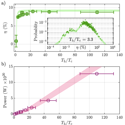
Figure 4: Engine efficiency and power. a) Measured efficiency (green circles) as a function of temperature ratio $T_{\mathrm{h}}/T_{\mathrm{c}}$. The efficiency rapidly saturates at around 9%, in agreement with our theory (shaded green line). The efficiency is calculated by taking the average of the heat-exchanged and work-done over all trajectories and then taking the ratio. The inset shows the distributions of efficiencies calculated within each trajectory at one temperature ratio, illustrating the highly stochastic nature of this quantity. Each green point represents a bin with 5 data points, and the shaded green region represents the standard deviation of the data within each bin. b) Measured power (purple circles) as a function of temperature ratio $T_{\mathrm{h}}/T_{\mathrm{c}}$, compared to our model (purple shaded region). Although the efficiency of the engine saturates with increasing temperature, the power output does not.

Macroscopic engines, as considered by Carnot 200 years ago, run by having the working medium receive energy (in the form of heat) from the hot reservoir, and it dumping less energy (also heat) into the cold reservoir, while extracting the difference in energy as useful work $W$. A key difference in microscopic engines is that the energetic exchanges are noticeably stochastic. Given the position-dependent temperature of the particle, quantification of heat exchange can be particularly subtle. Indeed, for the much explored overdamped case [42, 43, 44, 45, 46] it was found that the standard overdamped approximation can give fundamentally wrong predictions of the dissipated heat [42] when position-dependent noise is present. Here, we work in the underdamped regime. Following the well-established arguments by Sekimoto [47] we define heat at the single trajectory level as the back-action force of the environment on to the particle. Then the differential of heat exchanged in a single realisation is $\dj Q=\left(-\gamma_{g}mv+qE_{0}(z)\xi(t)\right)\circ\mathrm{d}z(t),$ and the differential average heat received by the particle becomes

$$\langle\dj Q\rangle=\left(-\gamma_{g}\langle{v^{2}}\rangle+D_{0}+D_{1}\langle{z}\rangle+D_{2}\langle{z^{2}}\rangle\right)m\mathrm{d}t.$$ (3)

We note that while the first two terms are the same as those that appear in the expression for heat of standard Brownian motion, the last two, entirely due to the position-dependent diffusion, are new. Interestingly, while heat dissipation is usually exclusively determined by the kinetic energy, Eq. (3) predicts that the potential energy also affects heat dissipation.

In Fig. 3 we plot the probability distributions of the measured heat that the levitated particle exchanges with the hot and cold reservoirs, over between 700-1400 individual realisations of the Stirling cycle. Panel a) highlights the extremely wide spread of heat exchanged with the environment, which increases dramatically with increasing temperature reaching many hundreds of $k_{\mathrm{B}}T_{\mathrm{c}}$. Panel b) gives an example distribution illustrating that the flow of heat can invert sign, flowing in the thermodynamically “wrong” direction. This effect becomes less pronounced at higher temperatures. We compare the measured heat distributions with the numerically obtained values from the model in Eq. (3), with (solid line) and without (dashed line) the additional diffusion terms $D_{1,2}$. We observe that the model in Eq. (3) better describes the experimentally observed distribution.

From the average heat and work we can obtain the average efficiency $\eta=\langle W\rangle/\langle Q_{\mathrm{h}}\rangle$ and power $P=\langle W\rangle/\tau$ of our engine cycle, where $\tau$ is the duration of the cycle. The experimentally obtained efficiency and power are plotted in Figs. 4 a) and b), respectively. We compare to the theoretical predictions from our model (shaded areas) which take into account the uncertainty in the model parameters (such as particle mass and estimated temperatures). We see that there is good agreement between the model and what we observe. We note that as the temperature ratio $T_{\mathrm{h}}/T_{\mathrm{c}}$ increases, the efficiency quickly saturates at a maximum value of $9\%$, whilst the power continues to increase. It is worth noting that the maximal efficiency obtained experimentally is smaller than the Carnot efficiency (about $99\%$), or even the more realistic finite power bound of Curzon-Ahlborn (about $90\%$). This is due to the fact that the Stirling cycle protocol we implement, a linear change of the harmonic frequency, is not the optimal protocol even for the case of standard underdamped Brownian motion [48]. Here we explore a new regime of operation, where the particle experiences position-dependent diffusion. Future research should address how to find an optimal cycle in this highly non-equilibrium situation [49, 48, 50, 51, 52].

Despite not being optimal, our engine efficiency of 9% is significantly higher than the 0.3% obtained in a single-atom engine following a similar protocol [27], due to the extreme temperature differences that we can achieve, pointing the way to potentially very high efficiencies. Comparing to experimental realizations of optimal engines such as in Ref. [28], similar efficiencies as ours are achieved.

Finally we can study the efficiency for each trajectory of the engine cycle (inset to Fig. 4a)). We see that the efficiency distribution displays extreme values, highlighting the highly stochastic nature of the engine. In some realizations the efficiency is negative. This is due to the fact that in some individual trajectories the flow of heat can be reversed and therefore the cycle is not actually operating as an engine. In other realizations efficiencies higher than 100% are achieved; as is well-known, one can stochastically violate the second law of thermodynamics at the single-trajectory level, obtaining efficiencies higher than Carnot predicted 200 years ago.

Discussion. In conclusion, we present a single-particle heat engine operating at extreme temperatures in excess of $10^{7}$ K, exhibiting large fluctuations in the heat exchanged with its environment and per-cycle efficiency. Levitation in a vacuum ensures the engine operates in the underdamped regime, and the use of electric fields to levitate the charged particle ensures a deep potential which provides linear dynamics even at very high temperatures.

Our experimental system shows great promise in its ability to simulate and explore not only high temperatures, but also the biologically relevant thermodynamic scenario of position-dependent diffusion (via spatially varying temperature), which is critical in describing the dynamics of our engine. Position-dependent diffusion is key to understanding, for example, protein folding [33] and mass transport [53] in biological settings. Moving forward, one can study non-Markovian energetics through the introduction of feedback [22, 54] and thermodynamic processes in the presence of non-White noise [41].

I Acknowledgements

This work has been supported by the European union (ERC Starting Grant 803277) and the Engineering and Physical Sciences Research Council (EP/S004777/1). JA and FC gratefully acknowledge funding from EPSRC (EP/R045577/1). JA thanks the Royal Society for the research grant on “First measurements of non-equilibrium fluctuations in the underdamped regime”.

II Supplementary information

II.1 Experimental setup

A $(4.8\pm 0.5)\,\mu$m diameter silica sphere (Bangs Laboratories, Inc.) is levitated at $(2.0\pm 0.4)\times 10^{-3}$ mbar using a custom-built linear Paul trap, shown in Fig. 1. The Paul trap consists of four trapping electrodes made from 3.0 mm diameter steel rods that are positioned such that they compose four corners of a square, with the centres of the rods on a circle of radius 5.0 mm. A signal generator (Stanford Research Systems DS345) generates a sinusoidally varying voltage which is amplified 1,000 times (TREK 10/10B-HS) and applied to one pair of diagonally opposed electrodes as, V = $V_{\rm{RF}}\rm{cos}(\omega_{\rm{RF}}t)$, where, $V_{\rm{RF}}$ = 1600 V, and, $\omega_{\rm{RF}}$ = $2\pi\times 1450$ Hz. The other pair of diagonally opposed electrodes have a small (0-10 V) DC voltage applied to centre the particle such that its micromotion is minimized.

The Paul trap has two cyclindrical endcap electrodes of diameter 1.0 mm which are aligned coaxially along the centre of the Paul trap, with a separation of 1.7 mm. A voltage supply (Stanford Research Systems SIM928) generates a DC voltage that is amplified 20 times (Falco Systems WMA-20) to give $U_{0}$ = 8.0 V on both electrodes, confining the particle in 3D.

The particle is introduced to the trap using Light Induced Acoustic Desorption (LIAD) [55, 56] at a pressure of $4\times 10^{-2}\,$mbar. Before launching, the dry sample of microparticles is sonicated for 30 minutes, and subsequently spread onto an aluminium sheet of 0.4 mm thickness, leaving a thin coating. A second sheet of aluminium is placed on top and rubbed across the sample, producing significant positive charge on the surface of the particle in excess of $10^{4}\,e$. We find a combination of this method and the mass-selectivity of the Paul trap leads to trapping of single spheres, as confirmed by light scattering.

A 532 nm laser beam (Vortran Stradus) of 40 mW power and a beam waist radius of $\sim 100\,\mu$m is used to image the particle, which scatters light onto the sensor of an Event Based Camera (EBC), (Prophessee EVK3 Gen4.1). The EBC contains an onboard proprietary tracking algorithm that tracks the particle motion in the plane of the camera in real time. This allows us to track the particle over hundreds of micrometres while retaining a position resolution of $30\,$nm Hz^-1/2. Further information on Event Based Imaging can be found in ref. [39].

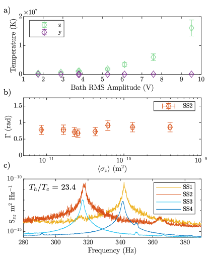
Figure 5: Technical details of the response of a levitated microparticle to the engine cycle. a) The temperature of the particle along the $z$-axis in response to white voltage noise with RMS amplitude $U_{T}$, green diamonds. The noise is applied to one endcap electrode, which produces a field which predominantly acts in the $z$-direction. This is verified through electric field simulations, and experimentally here by simultaneously monitoring the temperature along the $y$-axis, purple diamonds, which shows no significant response, giving us confidence that our engine operates in 1D only. b) The measured momentum damping rate $\Gamma=\gamma_{g}$ of a particle as the variance $\sigma_{z}$ of the motion along the $z$-axis increases due to increasing temperature, measured when the variance is maximized (in the hot bath with a loose trap, which we label SS2). This plot verifies that even at high temperatures, our particle remains in the linear part of the trapping potential; non-linearities broaden the spectral response [57]. c) The PSD of the particle motion along the $z$-axis at all four steady states of the engine cycle.

Calibration of our imaging system and calculation of particle charge is described in detail in ref. [39]. Once the system has been calibrated, the temperature of the particle can be calculated by analyzing the PSD or the position variance [11].

II.2 Experimental engine cycle

The Stirling engine protocol is generated by programming a function generator (Moku:Lab) to generate a voltage which is added to both endcap electrodes before amplification using a summing amplifier (Stanford Research Systems SIM980), resulting in a modified $U_{0}$. This changes the stiffness of the Paul trap, and shifts all of the secular frequencies of the levitated particle. Even though we only study the motion in the $z$-direction, it is critical that none of the motional frequencies cross $50\,$Hz (UK mains frequency) or its harmonics, since this pumps significant amounts of energy into the motion of the particle. This fact limits the amount which we can vary $f$ to $\sim 25\,$Hz, which is still over 30 linewidths.

The same function generator produces a signal which is used to both amplitude modulate white noise produced by a signal generator (Stanford Research Systems DS345), and trigger the EBC, which records the time that the hot bath is turned on and off in the data stream. This white noise with RMS amplitude $U_{T}$ is added to the DC voltage $U_{0}$ applied to a single endcap electrode before being amplified. The effective temperature of the levitated particle $T_{\mathrm{h}}$ is proportional to the square of $U_{T}$, see Fig. 5 (a), which also shows that this voltage noise only significantly heats the motion in the $z$-direction. We confirm that the particle remains in the linear part of the Paul trap potential by observing no change in the damping rate $\gamma_{g}$ with increasing motional standard deviation, Fig.5 (b). Furthermore, simulation in the ion-optics software SIMION verifies that our potential is harmonic over several hundred micrometers. The response of the particle in frequency space at each of the four steady states in the engine cycle is shown in Fig. 5 (c).

When the white noise voltage is turned off, the particle loses energy through interactions with the residual gas in the vacuum system. However, the equilibrium temperature when $U_{T}=0$ is not room-temperature, due to noise in the voltages used to levitate the particle, and is instead approximately 34,000 K.

II.3 Data processing and analysis

The output of the EBC gives the position of the particle over time in the $y-$ and $z-$directions, and contains trigger-marks for when the white voltage noise (heat bath) is switched on and off. Data was analysed in real time as the engine was running, and each cycle had a length of 135s. The engine cycle was repeated between 700 to 1400 times at each temperature. As we change the voltages $U_{0}$ on the endcap electrodes to change the particle’s frequency, the particle’s mean position shifts $\sim 1.7\,\mu$m due to unavoidable DC offsets present in the protocol and noise signals. The analysis assumes oscillation around an equilibrium position, and so for a given temperature, the trajectory of the particle averaged across all cycles is subtracted from each cycle. This is in effect a high-pass filter. No other filtering is performed on the data. Furthermore, temperature changes in the lab shift the measured position of the trap centre by around 7 $\mu$m over the course of several hours, as the imaging system moves slightly relative to the trap. Hence, the mean position of the particle in the first 1s of data is subtracted from each file to correct for this long term drift.

II.4 Theoretical model

As explained in the main text and in further detail in previous appendices, the two endcaps of the trap are used both for controlling the trapping frequency and applying the stochastic noise. Notably, the amplitude of the noise is comparable with the amplitude of the DC noise used to control the trap frequency ($U_{0}=8.0\,\mathrm{V}$ with ramp modulation of maximum amplitude of $1.5\,\mathrm{V}$ and the RMS value of the noise $U_{T}$ between $1.5\,\mathrm{V}$ – $9.5\,\mathrm{V}$). We therefore model the effect of the noise on the particle in two contributions: (i) a constant stochastic forcing of the particle (as is usually modelled in Brownian motion), and (ii) an effective stochastic fluctuation of the frequency of the harmonic trap. In such case, we can write the Langevin equation of motion

$$\dot{z} =v,$$ (4)

$$\dot{v} =-(\omega^{2}+\delta\omega^{2}\xi(t))z-\gamma_{g}v+F_{\mathrm{el}}\xi(t)+F_{\mathrm{gas}}(t),$$ (5)

where $F_{\mathrm{gas}}$ is the stochastic forcing due to collisions with the gas, $F_{\mathrm{el}}$ is the constant stochastic forcing due the electric noise, $\delta\omega^{2}$ characterizes the strength of the frequency fluctuations, and $\xi(t)$ is the Gaussian white noise associated with the electric noise such that $\langle\xi(t)\xi(t^{\prime})\rangle=2\delta(t-t^{\prime})$. Notice that here, the main difference from standard Brownian motion is the appearance of the multiplicative noise $\delta\omega^{2}$. Finally, note that here, without loss of generality, we take as centre of the harmonic trap the origin $z=0$.

The Langevin equation (5) can be rearranged as

$$\ddot{z}=-\omega^{2}z-\gamma_{g}v+F_{\mathrm{gas}}(t)+\frac{q}{m}E_{0}(z)\xi(t),$$ (6)

where $E_{0}(z)=(m/q)(F_{\mathrm{elec}}-\delta\omega^{2}z)$ is an effective position-dependent electric field that acts on the particle. From this Langevin equation, one can derive a corresponding Fokker-Planck equation for the probability density. To do so, we follow [40], where it is shown that given a general set of $N$-variable ($\vec{\eta}$) Langevin equations of the form

$$\dot{\eta}_{i}=h_{i}(\vec{\eta},t)+g_{ij}(\vec{\eta},t)\xi_{j}(t),\qquad i=1,\dots,N,$$ (7)

then, the associated probability distribution $\mathcal{P}(\vec{\eta},t)$ follows the Fokker-Planck equation

$$\frac{\partial\mathcal{P}(\vec{\eta},t)}{\partial t} =L^{\dagger}_{\mathrm{FP}}\mathcal{P}(\vec{\eta},t),$$ (8)

$$L^{\dagger}_{\mathrm{FP}} =-\frac{\partial}{\partial\eta_{i}}D^{(1)}_{i}(\vec{\eta},t)+\frac{\partial^{2}}{\partial\eta_{i}\eta_{j}}D^{(2)}_{ij}(\vec{\eta},t),$$

where the drift coefficients $D^{(1)}_{i}$ are given by

$$D^{(1)}_{i}(\vec{\eta},t)=h_{i}(\vec{\eta},t)+g_{kj}(\vec{\eta},t)\frac{\partial}{\partial\eta_{k}}g_{ij}(\vec{\eta},t),$$ (9)

while the diffusion coefficients $D^{(2)}_{ij}$ are

$$D^{(2)}_{ij}(\vec{\eta},t)=g_{ik}(\vec{\eta},t)g_{jk}(\vec{\eta},t).$$ (10)

Returning to our equations of motion (6), we can put them into the form of (7) with

$$\eta_{1}=x, \qquad\eta_{2}=v,$$ (11)

$$h_{1}(z,v,t)=v, \qquad h_{2}(z,v,t)=-\omega^{2}z-\gamma_{g}v,$$ (12)

$$g_{11}(z,v,t)=0, \qquad g_{12}(z,v,t)=0,$$ (13)

$$g_{21}(z,v,t)=F_{\mathrm{gas}}, \qquad g_{22}(z,v,t)=\frac{q}{m}E_{0}(z).$$ (14)

Therefore, the corresponding drift coefficients are

$$D_{1}^{(1)}(z,v,t)=v,\quad D_{2}^{(1)}(z,v,t)=-\omega^{2}z-\gamma_{g}v,$$ (15)

and the diffusion coefficients

$$D^{(2)}_{11}(z,v,t) =0,\quad D^{(2)}_{12}(z,v,t)=0,\quad$$ (16)

$$D^{(2)}_{21}(z,v,t) =0,\quad D^{(2)}_{22}(z,v,t)=F_{\mathrm{gas}}^{2}+\frac{q^{2}}{m^{2}}E_{0}^{2}(z).$$

Plugging this into (8) we obtain the Fokker-Planck equation (1) of the main text. Note that for $E_{0}(z)=(m/q)(F_{\mathrm{el}}-\delta\omega^{2}z)$, we obtain the diffusion coefficient

$$D^{(2)}_{22}(z,v,t)=D^{(2)}_{0}+D^{(2)}_{1}z+D^{(2)}z^{2},$$ (17)

with

$$D^{(2)}_{0} =F_{\mathrm{gas}}^{2}+F_{\mathrm{el}}^{2},$$ (18)

$$D^{(2)}_{1} =-2F_{\mathrm{el}}\delta\omega^{2},$$ (19)

$$D^{(2)}_{2} =\delta\omega^{4}.$$ (20)

Note that if the electric force term dominates over the gas collisions, $F_{\mathrm{gas}}^{2}\ll F_{\mathrm{el}}^{2}$, (which we expect to be valid due to the very low pressure of the system), then the $D_{0}\approx F_{\mathrm{el}}^{2}$ and the $D_{1}$ coefficient is fixed by the value of the $D_{0}$ and $D_{2}$ coefficients, i.e. $D_{1}\approx-2\sqrt{D_{0}D_{2}}$. This will be useful to allow us to remove one additional degree of freedom in the system parameters.

Now, taking the average over the ensemble of stochastic trajectories, we can obtain a closed set of differential equations for the particle’s dynamical first and second moments, $\langle z\rangle$, $\langle v\rangle$, and $\langle z^{2}\rangle$, $\langle v^{2}\rangle$, $\langle zv\rangle$. Then, the equations, describing the non-equilibrium dynamics of the particle, are

$$\frac{\mathrm{d}^{2}}{\mathrm{d}t^{2}}{\langle z\rangle} =-\omega^{2}\langle z\rangle-\gamma_{g}\langle v\rangle,$$ (21)

$$\frac{\mathrm{d}}{\mathrm{d}t}{\langle z^{2}\rangle} =2\langle zv\rangle,$$

$$\frac{\mathrm{d}}{\mathrm{d}t}\langle v^{2}\rangle =-2\omega^{2}\langle zv\rangle-2\gamma\langle v^{2}\rangle+2D_{0}+2D_{1}\langle z\rangle+2D_{2}\langle z^{2}\rangle,$$

$$\frac{\mathrm{d}}{\mathrm{d}t}\langle zv\rangle =\langle v^{2}\rangle-\omega^{2}\langle z^{2}\rangle-\gamma_{g}\langle zv\rangle.$$

Note that the equations of motion for the means follow exactly the dynamics of a standard damped harmonic oscillator, while the equations for the second moments differ from those of standard Brownian motion due to the appearance of the anomalous diffusion terms $D_{1}$ and $D_{2}$.

References

- Blickle and Bechinger [2012] V. Blickle and C. Bechinger, Realization of a micrometre-sized stochastic heat engine, Nature Physics 8, 143 (2012).
- Hänggi and Marchesoni [2009] P. Hänggi and F. Marchesoni, Artificial brownian motors: Controlling transport on the nanoscale, Rev. Mod. Phys. 81, 387 (2009).
- Franosch et al. [2011] T. Franosch, M. Grimm, M. Belushkin, F. M. Mor, G. Foffi, L. Forró, and S. Jeney, Resonances arising from hydrodynamic memory in brownian motion, Nature 478, 85 (2011).
- Bressloff and Newby [2013] P. C. Bressloff and J. M. Newby, Stochastic models of intracellular transport, Rev. Mod. Phys. 85, 135 (2013).
- Seifert [2012] U. Seifert, Stochastic thermodynamics, fluctuation theorems and molecular machines, Reports on Progress in Physics 75, 126001 (2012).
- Ciliberto [2017] S. Ciliberto, Experiments in stochastic thermodynamics: Short history and perspectives, Phys. Rev. X 7, 021051 (2017).
- Spesyvtseva and Dholakia [2016] S. E. S. Spesyvtseva and K. Dholakia, Trapping in a material world, ACS Photonics 3, 719 (2016).
- Gieseler and Millen [2018] J. Gieseler and J. Millen, Levitated nanoparticles for microscopic thermodynamics—a review, Entropy 20, 326 (2018).
- Millen and Gieseler [2018] J. Millen and J. Gieseler, Single particle thermodynamics with levitated nanoparticles, in Thermodynamics in the Quantum Regime: Fundamental Aspects and New Directions, edited by F. Binder, L. A. Correa, C. Gogolin, J. Anders, and G. Adesso (Springer International Publishing, Cham, 2018) pp. 853–885.
- Gieseler et al. [2021] J. Gieseler, J. R. Gomez-Solano, A. Magazzù, I. P. Castillo, L. P. García, M. Gironella-Torrent, X. Viader-Godoy, F. Ritort, G. Pesce, A. V. Arzola, K. Volke-Sepúlveda, and G. Volpe, Optical tweezers — from calibration to applications: a tutorial, Adv. Opt. Photon. 13, 74 (2021).
- Millen et al. [2020] J. Millen, T. S. Monteiro, R. Pettit, and A. N. Vamivakas, Optomechanics with levitated particles, Reports on Progress in Physics 83, 026401 (2020).
- Gonzalez-Ballestero et al. [2021] C. Gonzalez-Ballestero, M. Aspelmeyer, L. Novotny, R. Quidant, and O. Romero-Isart, Levitodynamics: Levitation and control of microscopic objects in vacuum, Science 374, eabg3027 (2021).
- Toyabe et al. [2010] S. Toyabe, T. Sagawa, M. Ueda, E. Muneyuki, and M. Sano, Experimental demonstration of information-to-energy conversion and validation of the generalized jarzynski equality, Nature Physics 6, 988 (2010).
- Bérut et al. [2012] A. Bérut, A. Arakelyan, A. Petrosyan, S. Ciliberto, R. Dillenschneider, and E. Lutz, Experimental verification of landauer’s principle linking information and thermodynamics, Nature 483, 187 (2012).
- Gomez-Solano et al. [2009] J. R. Gomez-Solano, A. Petrosyan, S. Ciliberto, R. Chetrite, and K. Gawedzki, Experimental verification of a modified fluctuation-dissipation relation for a micron-sized particle in a nonequilibrium steady state, Phys. Rev. Lett. 103, 040601 (2009).
- Rings et al. [2010] D. Rings, R. Schachoff, M. Selmke, F. Cichos, and K. Kroy, Hot brownian motion, Phys. Rev. Lett. 105, 090604 (2010).
- Ibáñez et al. [2024] M. Ibáñez, C. Dieball, A. Lasanta, A. Godec, and R. A. Rica, Heating and cooling are fundamentally asymmetric and evolve along distinct pathways, Nature Physics 20, 135 (2024).
- Li et al. [2010] T. Li, S. Kheifets, D. Medellin, and M. G. Raizen, Measurement of the instantaneous velocity of a brownian particle, Science 328, 1673 (2010).
- Gieseler et al. [2014] J. Gieseler, R. Quidant, C. Dellago, and L. Novotny, Dynamic relaxation of a levitated nanoparticle from a non-equilibrium steady state, Nature Nanotechnology 9, 358 (2014).
- Raynal et al. [2023] D. Raynal, T. de Guillebon, D. Guéry-Odelin, E. Trizac, J.-S. Lauret, and L. Rondin, Shortcuts to equilibrium with a levitated particle in the underdamped regime, Phys. Rev. Lett. 131, 087101 (2023).
- Hoang et al. [2018] T. M. Hoang, R. Pan, J. Ahn, J. Bang, H. T. Quan, and T. Li, Experimental test of the differential fluctuation theorem and a generalized jarzynski equality for arbitrary initial states, Phys. Rev. Lett. 120, 080602 (2018).
- Debiossac et al. [2020] M. Debiossac, D. Grass, J. J. Alonso, E. Lutz, and N. Kiesel, Thermodynamics of continuous non-markovian feedback control, Nature Communications 11, 1360 (2020).
- Militaru et al. [2021] A. Militaru, M. Innerbichler, M. Frimmer, F. Tebbenjohanns, L. Novotny, and C. Dellago, Escape dynamics of active particles in multistable potentials, Nature Communications 12, 2446 (2021).
- Rondin et al. [2017] L. Rondin, J. Gieseler, F. Ricci, R. Quidant, C. Dellago, and L. Novotny, Direct measurement of kramers turnover with a levitated nanoparticle, Nature Nanotechnology 12, 1130 (2017).
- Ricci et al. [2017] F. Ricci, R. A. Rica, M. Spasenović, J. Gieseler, L. Rondin, L. Novotny, and R. Quidant, Optically levitated nanoparticle as a model system for stochastic bistable dynamics, Nature Communications 8, 15141 (2017).
- Martínez et al. [2016] I. A. Martínez, É. Roldán, L. Dinis, D. Petrov, J. M. R. Parrondo, and R. A. Rica, Brownian carnot engine, Nature Physics 12, 67 (2016).
- Roßnagel et al. [2016] J. Roßnagel, S. T. Dawkins, K. N. Tolazzi, O. Abah, E. Lutz, F. Schmidt-Kaler, and K. Singer, A single-atom heat engine, Science 352, 325 (2016).
- Li et al. [2024] C. Li, S. Zhu, P. He, Y. Wang, Y. Zheng, K. Zhang, X. Gao, Y. Dong, and H. Hu, Realization of an all-optical underdamped stochastic stirling engine, Phys. Rev. A 109, L021502 (2024).
- Dago et al. [2021] S. Dago, J. Pereda, N. Barros, S. Ciliberto, and L. Bellon, Information and thermodynamics: Fast and precise approach to landauer’s bound in an underdamped micromechanical oscillator, Phys. Rev. Lett. 126, 170601 (2021).
- Dago et al. [2022] S. Dago, J. Pereda, S. Ciliberto, and L. Bellon, Virtual double-well potential for an underdamped oscillator created by a feedback loop, Journal of Statistical Mechanics: Theory and Experiment 2022, 053209 (2022).
- Dago et al. [2023] S. Dago, S. Ciliberto, and L. Bellon, Adiabatic computing for optimal thermodynamic efficiency of information processing, Proceedings of the National Academy of Sciences 120, e2301742120 (2023).
- Hummer [2005] G. Hummer, Position-dependent diffusion coefficients and free energies from bayesian analysis of equilibrium and replica molecular dynamics simulations, New Journal of Physics 7, 34 (2005).
- Best and Hummer [2010] R. B. Best and G. Hummer, Coordinate-dependent diffusion in protein folding, Proc. Natl. Acad. Sci. U. S. A. 107, 1088 (2010).
- Venable et al. [2019] R. M. Venable, A. Krämer, and R. W. Pastor, Molecular dynamics simulations of membrane permeability, Chemical Reviews 119, 5954 (2019).
- Whitford et al. [2013] P. C. Whitford, S. C. Blanchard, J. H. D. Cate, and K. Y. Sanbonmatsu, Connecting the kinetics and energy landscape of trna translocation on the ribosome, PLOS Computational Biology 9, 1 (2013).
- Verley et al. [2014] G. Verley, M. Esposito, T. Willaert, and C. Van den Broeck, The unlikely carnot efficiency, Nature Communications 5, 4721 (2014).
- Polettini et al. [2015] M. Polettini, G. Verley, and M. Esposito, Efficiency statistics at all times: Carnot limit at finite power, Phys. Rev. Lett. 114, 050601 (2015).
- Millen et al. [2014] J. Millen, T. Deesuwan, P. Barker, and J. Anders, Nanoscale temperature measurements using non-equilibrium brownian dynamics of a levitated nanosphere, Nature Nanotechnology 9, 425 (2014).
- Ren et al. [2022] Y. Ren, E. Benedetto, H. Borrill, Y. Savchuk, K. O’Flynn, M. Rashid, J. Millen, et al., Event-based imaging of levitated microparticles, Applied Physics Letters 121 (2022).
- Risken [1996] H. Risken, The Fokker-Planck Equation: Methods of Solution and Applications (Springer Berlin Heidelberg, 1996).
- Volpe and Wehr [2016] G. Volpe and J. Wehr, Effective drifts in dynamical systems with multiplicative noise: a review of recent progress, Reports on Progress in Physics 79, 053901 (2016).
- Celani et al. [2012] A. Celani, S. Bo, R. Eichhorn, and E. Aurell, Anomalous thermodynamics at the microscale, Physical Review Letters 109, 10.1103/physrevlett.109.260603 (2012).
- Ding et al. [2024] M. Ding, J. Wu, and X. Xing, Stochastic thermodynamics of brownian motion in temperature gradient, Journal of Statistical Mechanics: Theory and Experiment 2024, 033203 (2024).
- Marino et al. [2016] R. Marino, R. Eichhorn, and E. Aurell, Entropy production of a brownian ellipsoid in the overdamped limit, Physical Review E 93, 10.1103/physreve.93.012132 (2016).
- Sancho [2015] J. M. Sancho, Brownian colloids in underdamped and overdamped regimes with nonhomogeneous temperature, Physical Review E 92, 10.1103/physreve.92.062110 (2015).
- Polettini [2013] M. Polettini, Diffusion in nonuniform temperature and its geometric analog, Physical Review E 87, 10.1103/physreve.87.032126 (2013).
- Sekimoto [2010] K. Sekimoto, Stochastic Energetics (Springer Berlin Heidelberg, 2010).
- Dechant et al. [2017] A. Dechant, N. Kiesel, and E. Lutz, Underdamped stochastic heat engine at maximum efficiency, EPL (Europhysics Letters) 119, 50003 (2017).
- Schmiedl and Seifert [2007] T. Schmiedl and U. Seifert, Efficiency at maximum power: An analytically solvable model for stochastic heat engines, EPL (Europhysics Letters) 81, 20003 (2007).
- Ye et al. [2022] Z. Ye, F. Cerisola, P. Abiuso, J. Anders, M. Perarnau-Llobet, and V. Holubec, Optimal finite-time heat engines under constrained control, Physical Review Research 4, 10.1103/physrevresearch.4.043130 (2022).
- Abiuso et al. [2022] P. Abiuso, V. Holubec, J. Anders, Z. Ye, F. Cerisola, and M. Perarnau-Llobet, Thermodynamics and optimal protocols of multidimensional quadratic brownian systems, Journal of Physics Communications 6, 063001 (2022).
- Bauer et al. [2016] M. Bauer, K. Brandner, and U. Seifert, Optimal performance of periodically driven, stochastic heat engines under limited control, Physical Review E 93, 10.1103/physreve.93.042112 (2016).
- Nagai et al. [2020] T. Nagai, S. Tsurumaki, R. Urano, K. Fujimoto, W. Shinoda, and S. Okazaki, Position-dependent diffusion constant of molecules in heterogeneous systems as evaluated by the local mean squared displacement, Journal of Chemical Theory and Computation 16, 7239 (2020).
- Ren et al. [2024] Y. Ren, B. Siegel, R. Yin, M. Rashid, and J. Millen, Neuromorphic detection and cooling of microparticle arrays (2024), arXiv:2408.00661 [physics.ins-det] .
- Bykov et al. [2019] D. S. Bykov, P. Mestres, L. Dania, L. Schmöger, and T. E. Northup, Direct loading of nanoparticles under high vacuum into a Paul trap for levitodynamical experiments, Applied Physics Letters 115, 034101 (2019).
- Nikkhou et al. [2021] M. Nikkhou, Y. Hu, J. A. Sabin, and J. Millen, Direct and clean loading of nanoparticles into optical traps at millibar pressures, Photonics 8, 10.3390/photonics8110458 (2021).
- Gieseler et al. [2013] J. Gieseler, L. Novotny, and R. Quidant, Thermal nonlinearities in a nanomechanical oscillator, Nature Physics 9, 806 (2013).