Exact Matching in Correlated Networks with Node Attributes for Improved Community Recovery

Abstract

We study community detection in multiple networks whose nodes and edges are jointly correlated. This setting arises naturally in applications such as social platforms, where a shared set of users may exhibit both correlated friendship patterns and correlated attributes across different platforms. Extending the classical Stochastic Block Model (SBM) and its contextual counterpart (CSBM), we introduce the correlated CSBM, which incorporates structural and attribute correlations across graphs. To build intuition, we first analyze correlated Gaussian Mixture Models, wherein only correlated node attributes are available without edges, and identify the conditions under which an estimator minimizing the distance between attributes achieves exact matching of nodes across the two databases. For correlated CSBMs, we develop a two-step procedure that first applies $k$-core matching to most nodes using edge information, then refines the matching for the remaining unmatched nodes by leveraging their attributes with a distance-based estimator. We identify the conditions under which the algorithm recovers the exact node correspondence, enabling us to merge the correlated edges and average the correlated attributes for enhanced community detection. Crucially, by aligning and combining graphs, we identify regimes in which community detection is impossible in a single graph but becomes feasible when side information from correlated graphs is incorporated. Our results illustrate how the interplay between graph matching and community recovery can boost performance, broadening the scope of multi-graph, attribute-based community detection.

I Introduction

Identifying community labels of nodes from a given graph or database–often referred to as community recovery or community detection–is a fundamental problem in network analysis, with wide-ranging applications in machine learning, social network analysis, and biology. The principal insight behind many community detection approaches is that nodes within the same community are typically more strongly connected or share similar attributes compared to nodes in different communities. However, real-world networks frequently deviate from such idealized patterns due to noise or the presence of anomalous nodes whose behaviors do not conform to typical intra-community connectivity or attribute similarities, thereby complicating the community recovery process.

A variety of probabilistic models has been developed to provide rigorous frameworks for community detection. Among these, the Stochastic Block Model (SBM) introduced by Holland, Laskey, and Leinhardt [1] remains one of the most widely studied. In the classical SBM, $n$ nodes are partitioned into $r$ communities, and edges form with probability $p\in[0,1]$ between nodes in the same community, versus $q\in[0,p)$ between nodes in different communities. Such models capture community structures effectively in various settings–for example, social networks where edges represent friendships or interactions. In SBMs with $p=\frac{a\log n}{n}$, $q=\frac{b\log n}{n}$ for constants $a,b>0$ and $r=\Theta(1)$, it has been established in [2, 3, 4] that exact community recovery is information-theoretically achievable if and only if $\sqrt{a}-\sqrt{b}>\sqrt{r}$. Although SBMs incorporate only network structure, node attributes can play an equally important role in determining community memberships.

Since the standard SBM focuses on graph connectivity alone, it neglects potentially informative node attributes. To remedy this, the Contextual Stochastic Block Model (CSBM) includes node attributes alongside structural connectivity. For instance, in [5], the authors consider a two-community CSBM in which each node has a Gaussian-distributed attribute vector of dimension $d$, with mean either ${\boldsymbol{\mu}}$ or $-{\boldsymbol{\mu}}$ (depending on the node’s community) and covariance ${\boldsymbol{I}}_{d}$. This augmented framework leverages both graph structure and node attributes, leading to improved community recovery. Indeed, it is shown in [5] that the Signal-to-Noise Ratio (SNR), derived from both edges and attributes, governs the feasibility of exact community recovery, thereby demonstrating that combining these two sources of information can outperform methods relying on only one.

While CSBMs incorporate attributes in a single-network context, many real-world settings naturally feature multiple, correlated networks. For example, users often participate in more than one social platform (e.g., Facebook and LinkedIn), giving rise to correlated friendship relationships. However, due to privacy and security concerns, user identities are anonymized across different platforms, making it nontrivial to match corresponding users. This task, known as graph matching, is critical for leveraging correlated graphs for downstream tasks. Indeed, finding the exact correspondence between all nodes (i.e., exact matching) enables the construction of a combined graph by merging edges from both platforms, thereby facilitating more accurate community detection. Past research [6, 7] has shown that once exact matching is attainable in correlated SBMs, community recovery becomes easier than if only one graph were available. Moreover, Gaudio et al. [8] established precise information-theoretic limits for exact community recovery under correlated SBMs.

Building on these insights, this work addresses scenarios in which both edges and node attributes are correlated across multiple networks. For example, a user on platforms like Facebook and LinkedIn may exhibit similar friendship connections as well as comparable personal attributes. We posit that these correlated sources of information can significantly enhance community recovery. Concretely, we propose extending Contextual Stochastic Block Models to the correlated setting, resulting in correlated CSBMs.

As a preliminary step, we first investigate correlated Gaussian Mixture Models, which capture correlated attributes alone (i.e., without edges). By generalizing the database alignment techniques from [9, 10], we identify the conditions under which an estimator minimizing the distance between node attributes can reliably recover the underlying permutation $\pi_{*}:[n]\to[n]$, even when community memberships are initially unknown. For correlated CSBMs, we introduce a two-step algorithm for exact matching: in the first step, we apply the $k$-core matching approach [11], which leverages edge information to recover matching for $n-o(n)$ nodes; in the second step, we employ the minimum-distance estimator using the node attributes of the remaining unmatched nodes, thereby finalizing the alignment. We derive conditions where this two-step algorithm achieves exact matching.

Once the node alignment is established, merging the correlated edges yields a denser graph structure, while averaging correlated node attributes increases the effective SNR. Crucially, by aligning and combining graphs, we identify regimes in which community detection is impossible in a single graph but becomes feasible when side information from correlated graphs is incorporated. This strategy offers deeper insights into how the interplay between graph matching and community detection can improve overall performance. To the best of our knowledge, we are the first to investigate community recovery in correlated graphs that incorporate correlated node attributes, thereby broadening the scope of existing research on multi-graph and attribute-based community detection.

I-A Models

We introduce two new models to capture correlations: correlated Gaussian Mixture Models, which focus on node attributes alone, and correlated Contextual Stochastic Block Models, which integrate both node attributes and graph structure.

I-A1 Correlated Gaussian Mixture Models

First, we assign $d$ dimensional features (or attributes) to $n$ nodes. Let $V_{1}:=[n]$ denote the set of nodes in the first database, and for each node $i\in V_{1}$, the node attribute is given by

$${\boldsymbol{x}}_{i}=\boldsymbol{\mu}\sigma_{i}+{\boldsymbol{z}}_{i},$$ (1)

where $\boldsymbol{\mu}\in\mathbb{R}^{d}$, $\sigma_{i}\in\{-1,+1\}$ and ${\boldsymbol{z}}_{i}\sim\mathcal{N}(0,{\boldsymbol{I}}_{d})$ for all $i\in[n]$. Let ${\boldsymbol{\sigma}}:=\{\sigma_{i}\}_{i=1}^{n}$ be the vector of community labels associated with the nodes in $V_{1}$.

Next, for the node set $V_{2}:=[n]$, we assign the attribute

$${\boldsymbol{y}}_{i}=\boldsymbol{\mu}\sigma_{i}+\rho{\boldsymbol{z}}_{i}+\sqrt{1-\rho^{2}}{\boldsymbol{w}}_{i},$$ (2)

where $\rho\in[0,1]$ and ${\boldsymbol{w}}_{i}\sim\mathcal{N}(0,{\boldsymbol{I}}_{d})$ for all $i\in[n]$. Equivalently, for each $i\in[n]$, the pair $({\boldsymbol{x}}_{i},{\boldsymbol{y}}_{i})$ can be represented as

$$({\boldsymbol{x}}_{i},{\boldsymbol{y}}_{i})\sim\mathcal{N}\left(\left[\begin{matrix}\boldsymbol{\mu}\sigma_{i}&\boldsymbol{\mu}\sigma_{i}\end{matrix}\right],\Sigma_{d}\right),$$ (3)

where

$$\Sigma_{d}:=\left[\begin{matrix}{\boldsymbol{I}}_{d}&\text{diag}(\rho)\\ \text{diag}(\rho)&{\boldsymbol{I}}_{d}\\ \end{matrix}\right].$$ (4)

We view these assigned attributes as two “databases,” which can be represented by the matrices $X:=[{\boldsymbol{x}}_{1},{\boldsymbol{x}}_{2},\ldots,{\boldsymbol{x}}_{n}]^{\top}\in\mathbb{R}^{n\times d}$ and $Y^{\prime}:=[{\boldsymbol{y}}_{1},{\boldsymbol{y}}_{2},\ldots,{\boldsymbol{y}}_{n}]^{\top}\in\mathbb{R}^{n\times d}$. Finally, for a permutation $\pi_{*}:[n]\to[n]$, define $Y=[{\boldsymbol{y}}_{\pi_{*}(1)},{\boldsymbol{y}}_{\pi_{*}(2)},\ldots,{\boldsymbol{y}}_{\pi_{*}(n)}]^{\top}\in\mathbb{R}^{n\times d}$. We assume $\pi_{*}$ is uniformly distributed over $S_{n}$, the set of all permutations on $n$ elements. The community label vectors for $X$ and $Y$ are given by ${\boldsymbol{\sigma}}^{1}:={\boldsymbol{\sigma}}$ and ${\boldsymbol{\sigma}}^{2}:={\boldsymbol{\sigma}}\circ\pi_{*}^{-1}$, respectively. We write the resulting pair of databases as

$$(X,\,Y)\;\sim\;\text{CGMMs}\bigl{(}n,\boldsymbol{\mu},d,\rho\bigr{)}.$$

I-A2 Correlated Contextual Stochastic Block Models

Let $V=[n]$ be the vertex set, and let ${\boldsymbol{\sigma}}:=\{\sigma_{i}\}_{i=1}^{n}$ be the community labels, where each $\sigma_{i}\in\{-1,+1\}$ is drawn independently and uniformly at random. We generate a “parent” graph $G\sim\text{SBM}(n,p,q)$ with $p,q\in[0,1]$, $p>q$, and $q=\Theta(p)$ in the following manner. Partition $V$ into $V^{+}:=\{i\in[n]:\sigma_{i}=+1\}$ and $V^{-}:=\{i\in[n]:\sigma_{i}=-1\}$. If $\sigma_{u}\sigma_{v}=+1$, an edge $(u,v)$ is placed with probability $p$; if $\sigma_{u}\sigma_{v}=-1$, an edge is placed with probability $q$. The graph $G_{1}$ is then obtained by sampling every edge of $G$ independently with probability $s$. Similarly, $G^{\prime}_{2}$ is generated by the same sampling procedure, ensuring that $G_{1}$ and $G^{\prime}_{2}$ are subgraphs of $G$ with $\mathbb{P}\left\{(u,v)\in\mathcal{E}(G^{\prime}_{2})|(u,v)\in\mathcal{E}(G_{1})\right\}=s$ for all distinct $u,v\in[n]$, where $\mathcal{E}(G)$ denotes the edge set of graph $G$.

Each node in $G_{1}$ and $G^{\prime}_{2}$ is assigned correlated Gaussian attributes $\{{\boldsymbol{x}}_{i}\}$ and $\{{\boldsymbol{y}}_{i}\}$ as defined in (3), where $\boldsymbol{\mu}$ is uniformly distributed over the set $\bigl{\{}\boldsymbol{\mu}\in\mathbb{R}^{d}:\|\boldsymbol{\mu}\|^{2}=R\bigr{\}}$ for some $R>0$. Finally, $G_{2}$ is obtained by permuting the nodes of $G^{\prime}_{2}$ using $\pi_{*}:[n]\to[n]$. The community labels for $G_{1}$ and $G_{2}$ are given by ${\boldsymbol{\sigma}}^{1}:={\boldsymbol{\sigma}}$ and ${\boldsymbol{\sigma}}^{2}:={\boldsymbol{\sigma}}\circ\pi_{*}^{-1}$, respectively. Denoting the database (attribute) matrices by $X,Y^{\prime}$, and $Y$, and the adjacency matrices by $A,B^{\prime}$, and $B$, we denote the resulting graphs by

$$(G_{1},G_{2})\;\sim\;\text{CCSBMs}\bigl{(}n,p,q,s;\,R,d,\rho\bigr{)}.$$

I-B Prior Works

TABLE I: Characteristics of various models: This table summarizes the differences between the previous models and our two new models, depending on the existence of community structure, edges, node attributes, and/or correlated graphs.

Models	Communities	Edges	Node attributes	Correlated graphs
Correlated Erdős-Rényi graphs	-	O	-	O
Correlated Gaussian databases	-	-	O	O
Correlated Gaussian-Attributed Erdős-Rényi model	-	O	O	O
Stochastic Block Model	O	O	-	-
Gaussian Mixture Model	O	-	O	-
Contextual Stochastic Block Model	O	O	O	-
Correlated Stochastic Block Models	O	O	-	O
Correlated Gaussian Mixture Models (Ours)	O	-	O	O
Correlated Contextual Stochastic Block Models (Ours)	O	O	O	O

TABLE II: Comparison on the information-theoretic limits for exact matching and exact community recovery across various models: In the conditions for exact community recovery, we consider the cases with two communities and the parameter regimes where $p=\frac{a\log n}{n}$, $q=\frac{b\log n}{n}$, $c\log n=\frac{R^{2}}{R+d/n}$ and $c^{\prime}\log n=\frac{\left(\frac{2}{1+\rho}R\right)^{2}}{\frac{2}{1+\rho}R+d/n}$ for constants $a,b,c,c^{\prime}>0$. Our exact matching results also require $R\geq 2\log n+\omega(1)$ or $d=\omega(\log n)$, but these conditions have been omitted for simplicity.

	Models	Exact Graph Matching	Exact Community Recovery
[12]	Correlated Erdős-Rényi graphs	$nps^{2}\geq(1+\epsilon)\log n$	-
[9]	Correlated Gaussian databases	$\frac{d}{4}\log\frac{1}{1-\rho^{2}}\geq\log n+\omega(1)$	-
[13]	Correlated Gaussian-Attributed Erdős-Rényi model	$nps^{2}+\frac{d}{4}\log\frac{1}{1-\rho^{2}}\geq(1+\epsilon)\log n$	-
[4]	Stochastic Block Model	-	$s\frac{(\sqrt{a}-\sqrt{b})^{2}}{2}>1$
[14]	Gaussian Mixture Model	-	$c>2$
[5]	Contextual Stochastic Block Model	-	$\frac{s(\sqrt{a}-\sqrt{b})^{2}+c}{2}>1$
[7, 6]	Correlated Stochastic Block Models	$ns^{2}\frac{p+q}{2}\geq(1+\epsilon)\log n$	$\left(1-(1-s)^{2}\right)\frac{(\sqrt{a}-\sqrt{b})^{2}}{2}>1$
Our results	Correlated Gaussian Mixture Models	$\frac{d}{4}\log\frac{1}{1-\rho^{2}}\geq(1+\epsilon)\log n$	$c^{\prime}>2$
	Correlated Contextual Stochastic Block Models	$ns^{2}\frac{p+q}{2}+\frac{d}{4}\log\frac{1}{1-\rho^{2}}\geq(1+\epsilon)\log n$	$\frac{\left(1-(1-s)^{2}\right)\left(\sqrt{a}-\sqrt{b}\right)^{2}+c^{\prime}}{2}>1$

In Table I, we present various graph models–including our newly introduced ones–classified according to whether they incorporate community structure, edges, node attributes, or correlated graphs. Table II provides a summary of information-theoretic limits for graph matching in correlated graphs and community recovery in graphs with community structure, highlighting the performance gains achievable in our proposed models by incorporating correlated edges and/or node attributes.

I-B1 Graph Matching

Matching correlated random graphs

One of the most extensively studied settings for graph matching is the correlated Erdős–Rényi (ER) model, first proposed in [15]. In this model, the parent graph $G$ is drawn from $\mathcal{G}(n,p)$ (an ER graph), and $G_{1}$ and $G^{\prime}_{2}$ are obtained by independently sampling every edge of $G$ with probability $s$ twice. Cullina and Kiyavash [16, 17] provided the first information-theoretic limits for exact matching, showing that exact matching is possible if $nps^{2}\geq\log n+\omega(1)$ under the condition $p\leq O(1/(\log n)^{3})$. More recently, Wu et al. [12] showed that exact matching remains feasible whenever $p=o(1)$ and $nps^{2}\geq(1+\epsilon)\log n$ for any fixed $\epsilon>0$. However, these proofs rely on checking all permutations, yielding time complexity on the order of $\Theta(n!)$. Consequently, a significant effort has focused on more efficient algorithms. Quasi-polynomial time ($n^{O(\log n)}$) approaches were proposed in [18, 19], while polynomial-time algorithms in [20, 21, 22] achieve exact matching under $s=1-o(1)$. Recently, the first polynomial-time algorithms for constant correlation $s\geq\alpha$ (for a suitable constant $\alpha$) appeared in [23, 24], using subgraph counting or large-neighborhood statistics.

Graph matching under correlated Stochastic Block Models (SBMs), where the parent graph is an SBM, has also been investigated [25, 26]. Assuming known community labels in each graph, Onaran et al. [25] showed that exact matching is possible when $s(1-\sqrt{1-s^{2}})\frac{p+q}{2}\geq 3\log n$ for two communities. Cullina et al. [26] extended this to $r$ communities, where $p=\frac{a\log n}{n}$ and $q=\frac{b\log n}{n}$, demonstrating that exact matching holds if $s^{2}\frac{a+(r-1)b}{r}>2$. Notably, in the special case $p=q$, correlated SBMs reduce to correlated ER graphs; even under known labels, the bounds in [25, 26] differ from the information-theoretic limit in the correlated ER setting. Rácz and Sridhar [6] refined these results for $r=2$, proving that exact matching is possible if $s^{2}\,\frac{a+b}{2}>1$. Yang and Chung [7] generalized these findings to SBMs with $r$ communities, showing that exact matching holds if $ns^{2}\,\frac{p+(r-1)q}{r}\geq(1+\epsilon)\log n$, under mild assumptions. As before, achieving this bound requires a time complexity of $\Theta(n!)$. Yang et al. [27] designed a polynomial-time algorithm under constant correlation when community labels are known, and Chai and Rácz [28] recently devised a polynomial-time method that obviates label information.

Database alignment

Database alignment [9, 29, 30, 31] addresses the problem of finding a one-to-one correspondence between nodes in two “databases,” where each node is associated with correlated attributes. Similar to graph matching, various models have been proposed, among which the correlated Gaussian database model is popular. In this model, each pair of corresponding nodes $({\boldsymbol{x}}_{i},{\boldsymbol{y}}_{i})$ is drawn i.i.d. from $\mathcal{N}(\boldsymbol{\mu},\Sigma_{d})$, where $\boldsymbol{\mu}\in\mathbb{R}^{2d}$ and $\Sigma_{d}=\begin{bmatrix}{\boldsymbol{I}}_{d}&\text{diag}(\rho)\\ \text{diag}(\rho)&{\boldsymbol{I}}_{d}\end{bmatrix}.$ Dai et al. [9] showed that exact alignment is possible if $\tfrac{d}{4}\log\tfrac{1}{1-\rho^{2}}\geq\log n+\omega(1)$. Their method uses the maximum a posteriori (MAP) estimator, with a time complexity of $O(n^{2}d+n^{3})$.

Attributed graph matching

In many social networks, users (nodes) have both connections (edges) and personal attributes. The attributed graph alignment problem aims to match nodes across two correlated graphs while exploiting both edge structure and node features. In the correlated Gaussian-attributed ER model [13], the edges come from correlated ER graphs, and node attributes come from correlated Gaussian databases. It was shown that exact matching is possible if

$$nps^{2}+\frac{d}{4}\log\frac{1}{1-\rho^{2}}\geq(1+\epsilon)\log n,$$ (5)

indicating that the effective SNR is an additive combination of edge- and attribute-based signals.

Zhang et al. [32] introduced an alternative attributed ER pair model with $n$ user nodes and $m$ attribute nodes, assuming that the $m$ attribute nodes are pre-aligned. Edges between user nodes appear with probability $p$, while edges between users and attribute nodes appear with probability $q$. Similar to the correlated ER framework, edges are independently subsampled with probabilities $s_{p}$ and $s_{q}$ for user-user and user-attribute edges, respectively, and a permutation $\pi_{*}$ is applied to yield $G_{1}$ and $G_{2}$. Exact matching is possible if $nps_{p}^{2}+mqs_{q}^{2}\geq\log n+\omega(1)$. Polynomial-time algorithms for recovering $\pi_{*}$ in this setting have been explored in [33].

I-B2 Community Recovery in Correlated Random Graphs

Rácz and Sridhar [6] first investigated exact community recovery in the presence of two or more correlated networks. Focusing on correlated SBMs with $p=\frac{a\log n}{n}$ and $q=\frac{b\log n}{n}$ (for $a,b>0$) and two communities, they established conditions under which exact matching is possible. Once the exact matching is achieved, they construct a union graph $G_{1}\vee_{\pi_{*}}G_{2}\sim\text{SBM}\bigl{(}n,p(1-(1-s)^{2}),q(1-(1-s)^{2})\bigr{)}$, which is denser than the individual graphs $G_{1},G_{2}\sim\text{SBM}\bigl{(}n,ps,qs\bigr{)}$. By doing so, the threshold for exact community recovery becomes less stringent: while a single graph $G_{1}$ or $G_{2}$ requires $\sqrt{a}-\sqrt{b}>\tfrac{2}{s}$, the union graph only needs $\sqrt{a}-\sqrt{b}>\tfrac{2}{\sqrt{1-(1-s)^{2}}}$, illustrating a regime in which exact recovery is infeasible with a single graph but feasible with two correlated ones.

Although [6] narrowed the gap between achievability and impossibility for two-community correlated SBMs, Gaudio et al. [8] completely characterized the information-theoretic limit for exact recovery by leveraging partial matching, even in cases where perfect matching is not possible. Subsequent work has extended these ideas to correlated SBMs with more communities or more than two correlated graphs. Yang and Chung [7] generalized the results of [6] to SBMs with $r$ communities that may scale with $n$, while Rácz and Zhang [34] built on [8] to determine the exact information-theoretic threshold for community recovery in scenarios involving more than two correlated SBM graphs.

I-C Our Contributions

This paper introduces and analyzes two new models that jointly consider correlated graphs and correlated node attributes to better reflect hidden community structures. Specifically, we focus on correlated Gaussian Mixture Models (GMMs) and correlated Contextual Stochastic Block Models (CSBMs), as defined in Section I-A, with the ultimate goal of determining the conditions for exact community recovery. A key preliminary step is to establish exact matching–that is, to recover the one-to-one correspondence between the nodes of two correlated graphs–so that the second graph (or database) can serve as side information for community detection. We characterize the regimes under which exact matching is achievable or impossible in each proposed model.

In the correlated GMM setting, we adopt an estimator that minimizes the sum of squared distances between node attributes,

$$\hat{\pi}:=\operatorname*{arg\,min}_{\pi\in S_{n}}\sum_{i=1}^{n}\bigl{\lVert}{\boldsymbol{x}}_{i}-{\boldsymbol{y}}_{\pi(i)}\bigr{\rVert}^{2},$$ (6)

and establish threshold conditions for exact alignment. For the correlated CSBMs, we develop a two-step algorithm that first performs $k$-core matching using only edge information to match the majority of nodes, and then applies the distance-based attribute estimator (6) to align the remaining unmatched nodes. This two-step strategy, previously employed for correlated Gaussian-attributed Erdős–Rényi graphs [13], is shown here to be effective even when community labels are unknown. In particular, the $k$-core matching [11, 8, 35, 13], which selects the largest matching (the number of matched nodes) with a minimum degree of at least $k$ in the intersection graph under a particular permutation, turns out to be successfully recovery $n-o(n)$ nodes with a proper choice of $k$. We also analyze the MAP estimator to characterize the regimes in which exact matching becomes information-theoretically impossible.

Having established the conditions for exact matching, we then investigate exact community recovery in these correlated models. When matching is successful, one can merge the two correlated graphs by taking their union, thereby creating a denser graph, and average their correlated Gaussian attributes to reduce variance. Consequently, the achievable range for exact community detection expands relative to the scenario of having only a single graph or database, as illustrated in Figures 1 and 3. In particular, for correlated GMMs $(X,Y)\sim\text{CGMMs}\bigl{(}n,\boldsymbol{\mu},d,\rho\bigr{)}$ with $\|\boldsymbol{\mu}\|^{2}=R$, the effective signal-to-noise ratio for exact recovery increases from

$$\frac{R^{2}}{\,R+\tfrac{d}{n}\,}\quad\text{to}\quad\frac{\bigl{(}\tfrac{2}{1+\rho}\,R\bigr{)}^{2}}{\,\tfrac{2}{1+\rho}\,R+\tfrac{d}{n}\,},$$

while for the contextual SBMs $(G_{1},G_{2})\sim\text{CCSBMs}\bigl{(}n,p,q,s;R,d,\rho\bigr{)}$, the corresponding SNR improves from

$$\frac{s\bigl{(}\sqrt{a}-\sqrt{b}\bigr{)}^{2}+c}{\,2\,}\quad\text{to}\quad\frac{\bigl{(}1-(1-s)^{2}\bigr{)}\bigl{(}\sqrt{a}-\sqrt{b}\bigr{)}^{2}+c^{\prime}}{\,2\,},$$

where $c\log n=\frac{R^{2}}{\,R+d/n\,}$ and $c^{\prime}\log n=\frac{\bigl{(}\tfrac{2}{1+\rho}\,R\bigr{)}^{2}}{\,\tfrac{2}{1+\rho}\,R+d/n\,},$ compared to having only one contextual SBM ($G_{1}$ or $G_{2}$).

I-D Notation

For a positive integer $n$, write $[n]:=\{1,2,\ldots,n\}$. For a graph $G$ on vertex set $[n]$, let $\deg_{G}(i)$ be the degree of node $i$, and let $G\{M\}$ be the subgraph induced by $M\subseteq[n]$. Define $d_{\min}(G)$ as the minimum degree of $G$. Let $\mathcal{E}:=\{\{i,j\}:i,j\in[n],i\neq j\}$ be the set of all unordered vertex pairs. For a community label vector ${\boldsymbol{\sigma}}$, define

$$\mathcal{E}^{+}({\boldsymbol{\sigma}}):=\{\{i,j\}\in\mathcal{E}:\sigma_{i}\sigma_{j}=+1\}\quad\text{and}\quad\mathcal{E}^{-}({\boldsymbol{\sigma}}):=\{\{i,j\}\in\mathcal{E}:\sigma_{i}\sigma_{j}=-1\}.$$

Then $\mathcal{E}^{+}({\boldsymbol{\sigma}})$ and $\mathcal{E}^{-}({\boldsymbol{\sigma}})$ partition $\mathcal{E}$ into intra- and inter-community node pairs. Let $A,B^{\prime},B$ be the adjacency matrices of $G_{1},G^{\prime}_{2},G_{2}$, respectively, and let $X,Y^{\prime},Y$ be the corresponding databases of node attributes. Denote by $\vee$ and $\wedge$ the entrywise max and min, respectively. For a permutation $\pi$, define

$$(A\vee_{\pi}B)_{i,j}=\max\{A_{i,j},\,B_{\pi(i),\pi(j)}\}\quad\text{and}\quad(A\wedge_{\pi}B)_{i,j}=\min\{A_{i,j},\,B_{\pi(i),\pi(j)}\}.$$

For $v=[v_{1},\ldots,v_{k}]^{\top}\in\mathbb{R}^{k}$ and $i\in[k]$, let $v_{-i}$ be the vector obtained by removing $v_{i}$. For an event $E$, let $\mathds{1}(E)$ be its indicator. Write $\Phi(\cdot)$ for the tail distribution of a standard Gaussian. For two functions $f,g:[n]\to[m]$, define their overlap as $\mathbf{ov}(f,g):=\tfrac{1}{n}\sum_{i=1}^{n}\mathds{1}\bigl{(}f(i)=g(i)\bigr{)}$. Lastly, asymptotic notation $O(\cdot),o(\cdot),\Omega(\cdot),\omega(\cdot),\Theta(\cdot)$ is used with $n\to\infty$.

II Correlated Gaussian Mixture Models

In this section, we investigate the correlated Gaussian Mixture Models (GMMs) introduced in Section I-A1, with a primary goal of determining conditions for exact community recovery when two correlated databases are provided. Our approach consists of two steps: (i) establishing exact matching between the two databases, and (ii) merging the matched databases to identify regimes in which exact community recovery is significantly more tractable compared to using only a single database.

II-A Exact Matching on Correlated Gaussian Mixture Models

We begin by examining the requirements for exact matching in correlated GMMs. Theorem 1 below provides sufficient conditions under which an estimator (6) achieves perfect alignment with high probability.

Theorem 1 (Achievability for Exact Matching).

Let $(X,Y)\sim\textnormal{CGMMs}(n,\boldsymbol{\mu},d,\rho)$ as defined in Section I-A1. Suppose that either

$$\frac{d}{4}\log\frac{1}{1-\rho^{2}}\geq\log n+\omega(1)\quad\text{and}\quad\|\boldsymbol{\mu}\|^{2}\geq 2\log n+\omega(1),$$ (7)

or

$$\frac{d}{4}\log\frac{1}{1-\rho^{2}}\geq(1+\epsilon)\log n\quad\text{and}\quad d=\omega(\log n)$$ (8)

holds for an arbitrarily small constant $\epsilon>0$. Then there exists an estimator $\hat{\pi}(X,Y)$ such that $\hat{\pi}(X,Y)=\pi_{*}$ with high probability.

In correlated GMMs, the MAP estimator can be written as

$$\hat{\pi} =\operatorname*{arg\,max}_{\pi\in S_{n}}\mathbb{P}(\pi_{*}=\pi|X,Y)$$ (9)

$$\stackrel{{\scriptstyle(a)}}{{=}}\operatorname*{arg\,max}_{\pi\in S_{n}}\mathbb{P}(X,Y|\pi_{*}=\pi)$$

$$=\operatorname*{arg\,max}_{\pi\in S_{n}}\sum^{n}_{i=1}\left(-\|{\boldsymbol{x}}_{i}-\boldsymbol{\mu}\sigma_{i}\|^{2}+2\rho\langle{\boldsymbol{x}}_{i}-\boldsymbol{\mu}\sigma_{i},{\boldsymbol{y}}_{\pi(i)}-\boldsymbol{\mu}\sigma_{\pi(i)}\rangle-\|{\boldsymbol{y}}_{\pi(i)}-\boldsymbol{\mu}\sigma_{\pi(i)}\|^{2}\right)$$

$$=\operatorname*{arg\,max}_{\pi\in S_{n}}\sum^{n}_{i=1}\left(-\rho\|{\boldsymbol{x}}_{i}-{\boldsymbol{y}}_{\pi(i)}\|^{2}-(1-\rho)(\|{\boldsymbol{x}}_{i}\|^{2}+\|{\boldsymbol{y}}_{\pi(i)}\|^{2})\right)+f({\boldsymbol{\sigma}},{\boldsymbol{\sigma}}_{\pi})$$

$$=\operatorname*{arg\,min}_{\pi\in S_{n}}\sum^{n}_{i=1}\|{\boldsymbol{x}}_{i}-{\boldsymbol{y}}_{\pi(i)}\|^{2}-\frac{1}{\rho}f({\boldsymbol{\sigma}},{\boldsymbol{\sigma}}_{\pi}),$$

where

$$f\bigl{(}{\boldsymbol{\sigma}},{\boldsymbol{\sigma}}_{\pi}\bigr{)}=\sum_{i=1}^{n}\Bigl{(}2\langle{\boldsymbol{x}}_{i},\boldsymbol{\mu}\sigma_{i}\rangle+2\langle{\boldsymbol{y}}_{\pi(i)},\boldsymbol{\mu}\sigma_{\pi(i)}\rangle-2\rho\langle{\boldsymbol{x}}_{i},\boldsymbol{\mu}\sigma_{\pi(i)}\rangle-2\rho\langle{\boldsymbol{y}}_{\pi(i)},\boldsymbol{\mu}\sigma_{i}\rangle+2\rho\|\boldsymbol{\mu}\|^{2}\sigma_{i}\sigma_{\pi(i)}\Bigr{)}.$$

Step $(a)$ uses the fact that $\pi_{*}$ is uniformly distributed over $S_{n}$. Note also that $\sum_{i=1}^{n}\|{\boldsymbol{x}}_{i}\|^{2}+\|{\boldsymbol{y}}_{\pi(i)}\|^{2}$ is invariant under permutation $\pi$, ensuring this part does not affect the alignment decision. If the community labels ${\boldsymbol{\sigma}}$ and ${\boldsymbol{\sigma}}_{\pi}$ are known, then $f\bigl{(}{\boldsymbol{\sigma}},{\boldsymbol{\sigma}}_{\pi}\bigr{)}$ is also fixed, so the MAP estimator reduces exactly to the simpler distance-based estimator in (6). Even without known labels, the proof of Theorem 1 shows that (6) attains tight bounds under the conditions $\|\boldsymbol{\mu}\|^{2}\geq 2\log n+\omega(1)$ or $d=\omega(\log n)$; see Section VI for details.

Remark 1 (Interpretation of Conditions for Exact Matching).

Assume $d=o(n\log n)$. If $\|\boldsymbol{\mu}\|^{2}\geq(2+\epsilon)\log n$ for some $\epsilon>0$, then by [14], exact community recovery is already possible in each individual database $X$ or $Y$. In this situation, we only need to align nodes within the same community. Consequently, the distance-based estimator (6), which coincides with the MAP rule under known labels, matches nodes optimally. This explains the sufficiency of condition (7) for exact alignment when communities can first be recovered.

On the other hand, if $\|\boldsymbol{\mu}\|^{2}=O(\log n)$ is not large enough to recover community labels, exact matching can still be achieved by taking the condition (8). If $d=\omega(\log n)$, $\|{\boldsymbol{x}}_{i}-{\boldsymbol{y}}_{i}\|^{2}$, which originally follows the scaled chi-squared distribution, can be approximated as a normal distribution as follows:

$$\|{\boldsymbol{x}}_{i}-{\boldsymbol{y}}_{i}\|^{2}\stackrel{{\scriptstyle(d)}}{{\approx}}2\mathcal{N}((1-\rho)d,2(1-\rho)^{2}d).$$ (10)

Similarly, for different nodes within the same community, we obtain

$$\|{\boldsymbol{x}}_{i}-{\boldsymbol{y}}_{j}\|^{2}\stackrel{{\scriptstyle(d)}}{{\approx}}2\mathcal{N}(d,2d)\;\text{ for }i\neq j\text{ and }\sigma_{i}=\sigma_{j},$$ (11)

and for nodes in different communities,

$$\|{\boldsymbol{x}}_{i}-{\boldsymbol{y}}_{k}\|^{2}\stackrel{{\scriptstyle(d)}}{{\approx}}2\mathcal{N}(2\|\boldsymbol{\mu}\|^{2}+d,8\|\boldsymbol{\mu}\|^{2}+2d)\;\text{ for }i\neq k\text{ and }\sigma_{i}\neq\sigma_{k}.$$ (12)

If $d\gg\|\boldsymbol{\mu}\|^{2}$, then we can consider $\|{\boldsymbol{x}}_{i}-{\boldsymbol{y}}_{k}\|^{2}\stackrel{{\scriptstyle(d)}}{{\approx}}2\mathcal{N}(d,2d)$. Thus, through the approximations, for a fixed $i$, we can obtain that

$$\mathbb{P}\left(\|{\boldsymbol{x}}_{i}-{\boldsymbol{y}}_{i}\|^{2}\geq\|{\boldsymbol{x}}_{i}-{\boldsymbol{y}}_{j}\|^{2},\;\forall j\neq i\right)$$ (13)

$$\stackrel{{\scriptstyle(a)}}{{\leq}}n\mathbb{P}\left(\mathcal{N}((1-\rho)d,2(1-\rho)^{2}d)\geq\mathcal{N}(d,2d)\right)$$

$$\leq n\mathbb{P}\left(\mathcal{N}(0,2d(1+(1-\rho)^{2}))\geq\rho d\right)$$

$$\stackrel{{\scriptstyle(b)}}{{\leq}}\exp\left(\log n-\frac{1}{4}d\rho^{2}\cdot\frac{1}{1+(1-\rho)^{2}}\right).$$

The inequality $(a)$ holds by approximating (12) as (11) and taking a union bound over $j\neq i$, and the inequality $(b)$ holds by the tail bound of normal distribution (Lemma 19). Therefore, if $\frac{1}{4}d\rho^{2}\geq(1+(1-\rho)^{2})\log n+\omega(1)$, exact matching becomes achievable even with a greedy algorithm, which attempts to match each point to its nearest neighbor. If we consider the case where $\rho=o(1)$, the above condition becomes $\frac{1}{4}d\rho^{2}\geq 2\log n+\omega(1)$, while the bound in (8) is approximately $\frac{d}{4}\log\frac{1}{1-\rho^{2}}\approx\frac{1}{4}d\rho^{2}\geq(1+\epsilon)\log n$. The tighter bound in (8) is obtained by carefully analyzing the distance-based estimator (6).

We now state the matching impossibility result for correlated GMMs.

Theorem 2 (Impossibility for Exact Matching).

Let $(X,Y)\sim\textnormal{CGMMs}(n,\boldsymbol{\mu},d,\rho)$ be as in Section I-A1. Suppose either

$$\frac{d}{4}\log\frac{1}{1-\rho^{2}}\leq(1-\epsilon)\log n\quad\text{and}\quad 1\ll d=O(\log n),$$ (14)

for any small $\epsilon>0$, or

$$\frac{d}{4}\log\frac{1}{1-\rho^{2}}\leq\log n-\log d+C\quad\text{and}\quad\frac{1}{\rho^{2}}-1\leq\frac{d}{40}$$ (15)

for some positive constant $C>0$. Under either set of conditions, there is no estimator that can achieve exact matching with high probability.

Remark 2 (Gaps in Achievability and Converse Results).

Comparing Theorems 1 and 2 shows that the limiting condition for exact matching is roughly

$$\frac{d}{4}\log\frac{1}{1-\rho^{2}}\geq(1+\epsilon)\log n.$$ (16)

However, to attain achievability, we also require $\|\boldsymbol{\mu}\|^{2}\geq 2\log n+\omega(1)$ or $d=\omega(\log n)$. This gap may arise because the distance-based estimator (6) ignores the term $f({\boldsymbol{\sigma}},{\boldsymbol{\sigma}}_{\pi})$ in (9). This simplification enables us to recover the matching without relying on the knowledge of the community labels ${\boldsymbol{\sigma}}$ and ${\boldsymbol{\sigma}}_{\pi}$, but possibly at the cost of stricter requirements than the full MAP approach.

To prove the converse in Theorem 2, we show that the stated conditions imply failure of exact matching even if the community labels ${\boldsymbol{\sigma}}^{1}$ and ${\boldsymbol{\sigma}}^{2}$ are known, and a partial matching for all but $|V^{\prime}|$ nodes is revealed (where $V^{\prime}:=\{\,i\in[n]:\sigma_{i}=+1\}$). This reduces the task to a database alignment problem with $|V^{\prime}|$ nodes in correlated Gaussian databases, for which previous impossibility arguments in [9, 36] directly apply. A complete proof is given in Section VII.

II-B Exact Community Recovery in Correlated Gaussian Mixture Models

In [6], it was demonstrated that for correlated SBMs, once exact matching is achieved, combining correlated edges to form a denser union graph can extend the regime where exact community recovery is possible. Similarly, we now identify the conditions under which exact community recovery becomes feasible in correlated Gaussian Mixture Models (GMMs) when two correlated node-attribute databases are available.

Theorem 3 (Achievability for Exact Community Recovery).

Let $(X,Y)\sim\textnormal{CGMMs}(n,\boldsymbol{\mu},d,\rho)$ be as defined in Section I-A1. Suppose either (7) or (8) holds. If

$$\|\boldsymbol{\mu}\|^{2}\geq(1+\epsilon)\frac{1+\rho}{2}\biggl{(}1+\sqrt{1+\frac{2d}{n\log n}}\biggr{)}\log n$$ (17)

for an arbitrarily small constant $\epsilon>0$, then there exists an estimator $\hat{{\boldsymbol{\sigma}}}(X,Y)$ such that $\hat{{\boldsymbol{\sigma}}}(X,Y)={\boldsymbol{\sigma}}$ with high probability.

If exact matching is possible–or if $\pi_{*}$ is given–then the two correlated node attributes can be merged by taking their average. Specifically, if node $i\in[n]$ has attributes ${\boldsymbol{x}}_{i}$ and ${\boldsymbol{y}}_{\pi_{*}(i)}$, we form

$$\frac{{\boldsymbol{x}}_{i}+{\boldsymbol{y}}_{\pi_{*}(i)}}{2}=\boldsymbol{\mu}\sigma_{i}+\frac{(1+\rho){\boldsymbol{z}}_{i}+\sqrt{1-\rho^{2}}{\boldsymbol{w}}_{i}}{2},$$ (18)

where ${\boldsymbol{x}}_{i}$ and ${\boldsymbol{y}}_{i}$ are defined in (1) and (2), respectively. Since ${\boldsymbol{z}}_{i}$ and ${\boldsymbol{w}}_{i}$ are independent $d$-dimensional Gaussian vectors, $\frac{(1+\rho){\boldsymbol{z}}_{i}+\sqrt{1-\rho^{2}}{\boldsymbol{w}}_{i}}{2}$ is a $d$-dimensional Gaussian with mean $0$ and covariance $\frac{1+\rho}{2}\,{\boldsymbol{I}}_{d}$. Therefore, the averaged attribute has the same mean as the individual node attributes but a smaller variance. By applying known results for Gaussian Mixture Models [14, 5] to this averaged feature, we establish Theorem 3. A detailed proof is provided in Section VIII.

Remark 3 (Comparison with Standard GMM Results).

When only $X$ is available, [14, 5] showed that exact community recovery in a Gaussian Mixture Model requires

$$\lVert\boldsymbol{\mu}\rVert^{2}\geq(1+\epsilon)\left(1+\sqrt{1+\frac{2d}{n\log n}}\right)\log n.$$ (19)

Comparing (17) with (19) reveals that $\|\boldsymbol{\mu}\|^{2}$ can be smaller by a factor of $\tfrac{1+\rho}{2}$ when the correlated database $Y$ is available and we can form the combined feature (18) via exact matching. From (8), such a gain is particularly relevant in the regime $d=\omega(\log n)$. If $d=O(\log n)$, then to satisfy (7) we need $\|\boldsymbol{\mu}\|^{2}\geq 2\log n+\omega(1)$ for exact matching, which can exceed the threshold (17) for community recovery. Hence, in low-dimensional regimes, the advantage of incorporating the second database $Y$ is constrained by the stricter requirement on $\|\boldsymbol{\mu}\|^{2}$ for alignment.

We now provide the converse result, stating when exact community recovery is not possible in correlated GMMs.

Theorem 4 (Impossibility for Exact Community Recovery).

Let $(X,Y)\sim\textnormal{CGMMs}(n,\boldsymbol{\mu},d,\rho)$ as in Section I-A1. Suppose

$$\lVert\boldsymbol{\mu}\rVert^{2}\leq(1-\epsilon)\frac{1+\rho}{2}\left(1+\sqrt{1+\frac{2d}{n\log n}}\right)\log n$$ (20)

for an arbitrarily small constant $\epsilon>0$. Then, there is no estimator that achieves exact community recovery with high probability.

The proof of Theorem 4 follows the same reasoning as in Theorem 8 for the special case $p,q=0$, thus it can be viewed as a corollary of that result.

Remark 4 (Information-Theoretic Gaps in Exact Community Recovery).

Theorem 3 assumes that either (7) or (8) is satisfied to ensure exact matching. This raises a natural question: if matching is not feasible (i.e., $\tfrac{d}{4}\log\tfrac{1}{1-\rho^{2}}<\log n$), must exact community recovery also remain impossible, even if (17) holds? Addressing this question when exact matching is precluded is an interesting open problem, discussed further in Section V.

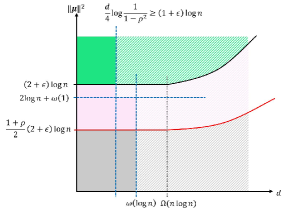
Figure 1: Conditions for exact community recovery (solid lines) and exact matching (dashed lines) in Gaussian Mixture Models (GMMs). The green region indicates where exact recovery is possible with a single GMM $X$, whereas the gray region shows where recovery is not possible even with correlated GMMs $(X,Y)$. The pink + green region (above the red curve) highlights where two correlated attributes $X$ and $Y$ enable exact recovery. The blue dashed line corresponds to conditions (7) and (8) for exact matching, with striped areas indicating parameter regimes where matching is feasible. Notably, the striped pink region represents cases where $X$ alone is insufficient for community recovery, but $(X,Y)$ together can achieve it, demonstrating the benefit of using correlated attributes.

Figure 1 illustrates the threshold conditions for both exact matching and exact community recovery in correlated Gaussian Mixture Models. It visually highlights how the addition of correlated node attributes expands the parameter regime where community detection becomes feasible.

III Correlated Contextual Stochastic Block Models

In this section, we consider the correlated Contextual Stochastic Block Models (CSBMs) introduced in Section I-A2. Similar to Section II, we first establish the conditions for exact matching and then derive the conditions for exact community recovery, assuming we can perfectly match the nodes between the two correlated graphs.

III-A Exact Matching

The following theorem provides sufficient conditions for exact matching in correlated CSBMs.

Theorem 5 (Achievability for Exact Matching).

Let $(G_{1},G_{2})\sim\textnormal{CCSBMs}(n,p,q,s;R,d,\rho)$ be as defined in Section I-A2, and suppose

$$p\leq O\left(\frac{1}{e^{(\log\log n)^{3}}}\right),$$ (21)

as well as

$$R\geq 2\log n+\omega(1)\text{ or }d=\omega(\log n)$$ (22)

holds. If

$$ns^{2}\frac{p+q}{2}+\frac{d}{4}\log\frac{1}{1-\rho^{2}}\geq(1+\epsilon)\log n$$ (23)

for an arbitrarily small constant $\epsilon>0$, then there exists an estimator $\hat{\pi}(G_{1},G_{2})$ such that $\hat{\pi}(G_{1},G_{2})=\pi_{*}$ with high probability.

In [6, 35, 7], it was shown that for correlated SBMs, exact matching is possible if the average degree of the intersection graph $ns^{2}\tfrac{p+q}{2}$ exceeds $\log n$. Hence, we focus on the regime $ns^{2}\tfrac{p+q}{2}=O(\log n)$, where we employ a two-step approach. First, we use $k$-core matching to align a large fraction of the nodes via edge information alone; the $k$-core approach has been extensively studied in [11, 8, 35] and is adapted here to handle more general regimes of $p$ and $q$. By choosing an appropriate $k$, we obtain a partial matching that is both large (in terms of the number of matched nodes) and accurate (no mismatches). The remaining unmatched node pairs follow the correlated Gaussian Mixture Model framework, so we apply Theorem 1 to match those residual pairs via the node-attribute estimator.

Remark 5 (Interpretation of Conditions for Exact Matching).

Condition (21) ensures that the $k$-core algorithm yields the correct matching for nodes within the $k$-core of $G_{1}\wedge_{\pi_{*}}G_{2}$. Condition (22) is required for matching the remaining nodes using node attributes. The combined inequality (23) highlights the benefit of leveraging both edge and node-attribute correlations. As a baseline, if $d=0$ (no node attributes), the model reduces to correlated SBMs, and (23) becomes $ns^{2}\tfrac{p+q}{2}\geq(1+\epsilon)\,\log n$, matching the exact-matching threshold in [6, 35, 7]. Conversely, if $p=q=0$ (no edges), the model is just correlated GMMs, and (23) becomes $\frac{d}{4}\log\!\bigl{(}\tfrac{1}{1-\rho^{2}}\bigr{)}\geq(1+\epsilon)\log n$, consistent with Theorem 1.

Theorem 6 (Impossibility for Exact Matching).

Let $(G_{1},G_{2})\sim\textnormal{CCSBMs}(n,p,q,s;R,d,\rho)$ be as in Section I-A2, and assume $ps^{2}=o(1)$. Suppose either

$$ns^{2}\frac{p+q}{2}+\frac{d}{4}\log\frac{1}{1-\rho^{2}}\leq(1-\epsilon)\log n\text{ and }1\ll d=O(\log n)$$ (24)

for arbitrarily small $\epsilon>0$, or

$$ns^{2}\frac{p+q}{2}+\frac{d}{4}\log\frac{1}{1-\rho^{2}}\leq\log n-\log d-\omega(1)\text{ and }\frac{1}{\rho^{2}}-1\leq\frac{d}{40}.$$ (25)

Then no estimator can achieve exact matching with high probability.

To prove Theorem 6, we show that even a MAP estimator fails when we provide $G_{1}$, $G_{2}$, the community labels ${\boldsymbol{\sigma}}^{1}$ and ${\boldsymbol{\sigma}}^{2}$ for each graph, the mean vector $\boldsymbol{\mu}$, and partial knowledge of $\pi_{*}$ on all but the set

$$\mathcal{H}_{*}:=\left\{i\in[n]:\forall j\in[n],A_{ij}B_{\pi_{*}(i)\pi_{*}(j)}=0\right\}$$ (26)

which consists of isolated nodes in the intersection graph $A\wedge_{\pi_{*}}B$. Section X contains the detailed argument.

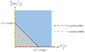
Figure 2: The region in blue indicates where exact matching is possible in correlated CSBMs, and the gray region shows where matching is infeasible. The red dashed line ($d=0$) captures the special case of correlated SBMs, while the yellow dashed line ($p=q=0$) represents correlated GMMs. Each dashed line intersects the boundary of the blue region at its respective matching threshold, thus recovering the known results for correlated SBMs and correlated GMMs.

The figure 2 illustrates the parameter regions where exact node matching is (blue area) and is not (gray area) achievable in correlated Contextual Stochastic Block Models. It also highlights how removing either edges ($p,q=0$) or node attributes ($d=0$) reduces the region of feasible matching to the thresholds for correlated GMMs and correlated SBMs, respectively.

III-B Exact Community Recovery

In [4], it was shown that if $p,q=\omega\bigl{(}\tfrac{\log n}{n}\bigr{)}$ ($p>q$), then exact community recovery in a single CSBM graph $G_{1}$ is achievable using only edge information. Likewise, it was shown in [14, 5] that if the effective SNR $\frac{R^{2}}{R+d/n}=\omega(\log n)$ where $\|\boldsymbol{\mu}\|^{2}=R,$ then exact community recovery is possible using only node attributes in $G_{1}$. Accordingly, for correlated CSBMs, we focus on the setting

$$p=\frac{a\log n}{n},\quad q=\frac{b\log n}{n},\quad\frac{R^{2}}{R+d/n}=c\log n,\quad\frac{\left(\frac{2}{1+\rho}R\right)^{2}}{\frac{2}{1+\rho}R+d/n}=c^{\prime}\log n$$ (27)

for positive constants $a,b,c,c^{\prime}$. The last term in (27) represents the SNR for the averaged correlated Gaussian attributes in (18). Under these assumptions, we have the following feasibility and infeasibility results for exact community recovery.

Theorem 7 (Achievability for Exact Community Recovery).

Let $(G_{1},G_{2})\sim\textnormal{CCSBMs}\bigl{(}n,p,q,s;R,d,\rho\bigr{)}$ be as in Section I-A2. Suppose conditions (21), (22), and (23) hold, and also assume (27). If

$$\frac{\bigl{(}1-(1-s)^{2}\bigr{)}\,\bigl{(}\sqrt{a}-\sqrt{b}\bigr{)}^{2}+c^{\prime}}{\,2\,}\;>\;1,$$ (28)

then there exists an estimator $\hat{{\boldsymbol{\sigma}}}(G_{1},G_{2})$ such that $\hat{{\boldsymbol{\sigma}}}(G_{1},G_{2})={\boldsymbol{\sigma}}$ with high probability.

When exact matching is achievable, we can construct a new Contextual Stochastic Block Model by forming a denser union graph $G_{1}\vee_{\pi_{*}}G_{2}$ whose edges follow $\textnormal{SBM}\bigl{(}n,p(1-(1-s)^{2}),q(1-(1-s)^{2})\bigr{)}$, and by assigning to each node the averaged correlated attribute from (18). Applying the techniques of [5] to this merged structure establishes Theorem 7.

Remark 6 (Comparison with the Single-Graph Setting).

Abbe et al. [5] showed that exact community recovery in a single CSBM $G_{1}$ is possible if

$$\frac{s\bigl{(}\sqrt{a}-\sqrt{b}\bigr{)}^{2}+c}{2}>1.$$

When two correlated graphs $G_{1}$ and $G_{2}$ are available, an exact matching (if feasible) allows one to form a denser union graph from the correlated edges and to average the correlated attributes. This increases the effective SNR term to

$$\frac{\bigl{(}1-(1-s)^{2}\bigr{)}\bigl{(}\sqrt{a}-\sqrt{b}\bigr{)}^{2}+c^{\prime}}{2},$$

thereby relaxing the threshold to the condition in (28). A detailed proof of Theorem 7 can be found in Section XI.

Theorem 8 (Impossibility for Exact Community Recovery).

Let $(G_{1},G_{2})\sim\textnormal{CCSBMs}\bigl{(}n,p,q,s;R,d,\rho\bigr{)}$ be as in Section I-A2, and assume (27). If

$$\frac{\bigl{(}1-(1-s)^{2}\bigr{)}\bigl{(}\sqrt{a}-\sqrt{b}\bigr{)}^{2}+c^{\prime}}{2}<1,$$ (29)

then no estimator can achieve exact community recovery with high probability.

The proof of Theorem 8 resembles the simulation argument used in Theorem 3.4 of [6], where one constructs a graph $\mathrm{H}$ to mirror $(G_{1},G_{2})$. By showing that exact community recovery in $\mathrm{H}$ is impossible under (29), it follows that $(G_{1},G_{2})$ also fails to admit exact community recovery. A detailed proof is given in Section XII.

Figure 3 visualizes the parameter ranges under which community recovery is possible or impossible in correlated CSBMs. It highlights how adding correlated node attributes and edges can expand the regime where exact community detection succeeds.

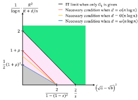
Figure 3: Green region: exact community recovery is possible using a single graph $G_{1}$. Gray region: exact recovery remains impossible even when two correlated graphs $(G_{1},G_{2})$ are given. The red, yellow, and blue lines mark necessary conditions for exact recovery, depending on the dimensional regime of $d$. In particular, the pink area indicates where single-graph recovery fails, but having two correlated graphs $(G_{1},G_{2})$ can enable exact recovery if exact matching is feasible.

Remark 7 (SNR of Node Attributes).

Suppose

$$\frac{\left(\frac{2}{1+\rho}R\right)^{2}}{\tfrac{2}{1+\rho}R+\tfrac{d}{n}}=2\,\log n\quad\Longrightarrow\quad\frac{2}{1+\rho}\,R\approx\sqrt{\frac{2d}{n}\,\log n}\;\;\text{or}\;\;2\log n,$$

depending on whether $d$ dominates $n\log n$ or not. In the high-dimensional regime $d=\omega(n\log n)$, we obtain $\frac{2}{1+\rho}\,R\approx\sqrt{\tfrac{2d}{n}\log n}$, yielding $\frac{R^{2}}{\,R+\tfrac{d}{n}\,}\approx\tfrac{1}{2}(1+\rho)^{2}\log n$. In contrast, if $d=o(n\log n)$, we have $\frac{2}{1+\rho}\,R\approx 2\log n$, so $\frac{R^{2}}{\,R+\tfrac{d}{n}\,}\approx(1+\rho)\log n$. Finally, in the intermediate case $d=\Theta(n\log n)$, the achievable SNR lies between these two extremes. These scenarios explain how the $y$-intercept in Figure 3 varies with respect to $d$.

IV Outline of the Proof

Without loss of generality, let $\pi_{*}:[n]\to[n]$ be the identity permutation. In this section, we outline the proofs of exact matching for the two proposed models.

IV-A Proof Sketch of Theorem 1

We begin by explaining how Theorem 1 can be established via the estimator in (6). The argument closely follows the ideas of [10], adapted to our setting.

Define

$$Z_{ij}:=\lVert{\boldsymbol{x}}_{i}-{\boldsymbol{y}}_{j}\rVert^{2}.$$ (30)

Then the estimator (6) can be rewritten as

$$\hat{\pi}=\operatorname*{arg\,min}_{\pi\in S_{n}}\sum\limits_{i=1}^{n}Z_{i\pi(i)}.$$ (31)

Let

$$\mathcal{M}:=\{i\in[n]:\hat{\pi}(i)\neq\pi_{*}(i)\}.$$ (32)

be the set of mismatched nodes. Our goal is to show that $\mathbb{P}\bigl{(}|\mathcal{M}|=0\bigr{)}=1-o(1)$.

Consider the event

$$\mathcal{F}_{t}=\left\{\sum_{k=1}^{t}Z_{i_{k}i_{k}}\geq\sum_{k=1}^{t}Z_{i_{k}i_{k+1}}\right\},$$ (33)

where $i_{1},\ldots,i_{t}$ are $t$ distinct nodes in $[n]$, and $i_{t+1}=i_{1}$. We will show that the probability of $\mathcal{F}_{t}$ is sufficiently small if either (7) or (8) holds. Denote this upper bound by $f(t)$. Since there are ${n\choose t}(t-1)!$ ways to choose $t$ distinct nodes, we obtain

$$\mathbb{E}(|\mathcal{M}|)\leq\sum\limits_{t=2}^{n}f(t){n\choose t}(t-1)!$$ (34)

where $t=1$ cannot yield a mismatch by itself. If $f(t)$ is made sufficiently small, it follows that $\mathbb{E}\bigl{(}|\mathcal{M}|\bigr{)}=o(1)$, and by Markov’s inequality, $\mathbb{P}\bigl{(}|\mathcal{M}|=0\bigr{)}=1-o(1)$. Achieving a suitably small $f(t)$ necessitates either (7) or (8). A rigorous proof can be found in Section VI.

IV-B Proof Sketch of Theorem 5

Exact matching in correlated CSBMs is proved via a two-step algorithm:

1. $k$-core matching using edges: We choose

   $$k=\frac{\log n}{(\log\log n)^{2}}\vee\frac{nps^{2}}{(\log nps^{2})^{2}}.$$

   Applying $k$-core matching with this $k$ matches $n-o(n)$ nodes correctly, leaving a set $F$ of unmatched nodes satisfying

   $$|F|\leq n^{1-\frac{ns^{2}(p+q)}{2\log n}+o(1)}.$$ (35)

2. Matching the remainder via node attributes: The remaining unmatched nodes in $F$ form a correlated Gaussian Mixture Model. Under assumptions (22) and (23), Theorem 1 applies, ensuring that these nodes can also be matched correctly using their node attributes.

A full proof of Theorem 5, detailing each step, can be found in Section IX.

V Discussion and Open Problems

In this work, we studied the problem of community recovery in the presence of two correlated networks. We introduced, for the first time, Correlated Gaussian Mixture Models (CGMMs), which focus on correlated node attributes, and Correlated Contextual Stochastic Block Models (CCSBMs), which leverage both correlated node attributes and edges. We showed that, while exact community recovery may be impossible for a single network, there are parameter regimes in which having a second, correlated network serves as valuable side information, thereby making exact community recovery feasible. In particular, we found that sufficiently high-dimensional node attributes–on the order of $\omega(\log n)$–can enable effective recovery.

To obtain these results, we first identified conditions for exact matching between the two networks. Notably, exact matching is easier to achieve when both node attributes and edges are correlated, compared to scenarios where only one is available. Below, we discuss several open problems stemming from our study.

V-1 Closing the information-theoretic gap for exact matching

Consider first the case of Correlated Gaussian Mixture Models. In Theorem 1, either $d=\omega(\log n)$ or $\|\boldsymbol{\mu}\|^{2}\geq 2\log n+\omega(1)$ must hold for exact matching. In contrast, in the community-free correlated Gaussian database model (i.e., $\boldsymbol{\mu}=0$), Dai et al. [9] showed that exact matching is possible with $\frac{d}{4}\log\frac{1}{1-\rho^{2}}\geq\log n+\omega(1)$ without further constraints on $d$. Meanwhile, Theorem 2 leaves some gaps, especially for $d=\Omega(n)$. We hypothesize that higher-dimensional attributes should make exact matching progressively easier, suggesting that $\frac{d}{4}\log\frac{1}{1-\rho^{2}}\geq(1+\epsilon)\log n$ may indeed be the core information-theoretic threshold, even without additional conditions on $\boldsymbol{\mu}$ and $d$. Resolving this would also address the same gap in the CCSBM setting, since the latter relies on CGMMs for unmatched nodes.

V-2 Closing the information-theoretic gap for exact community recovery

Theorems 3 and 7 establish achievable regions for exact community recovery in CGMMs and CCSBMs under the assumption that exact matching is possible. Comparing these to the converse results (Theorems 4 and 8) reveals that the stated conditions are not necessarily tight. Thus, it is natural to ask whether exact matching is truly needed for exact community recovery. Indeed, in correlated SBMs, Rácz and Sridhar [6] used exact matching to derive conditions for community recovery, whereas Gaudio et al. [8] refined the threshold by using partial matching (e.g., $k$-core). Similarly, one might conjecture that for correlated GMMs there exists a constant $\kappa$ such that, even if $\frac{d}{4}\log\frac{1}{1-\rho^{2}}\geq(1-\kappa)\log n$ there exists an estimator $\tilde{{\boldsymbol{\sigma}}}$ that can exactly recover ${\boldsymbol{\sigma}}$ even without full matching. Exploring this possibility is an intriguing open problem.

V-3 Generalizing to more communities

Our analysis has focused on the simplest case of two communities. A natural next step is to consider models with $r\geq 2$ communities. It would be interesting to investigate whether the conditions for exact matching and exact community recovery generalize in a straightforward manner or require fundamentally new techniques.

V-4 Multiple correlated graphs

We have considered only two correlated graphs. Another direction is to explore the setting where more than two correlated graphs are given. For example, Ameen and Hajek [37] established exact matching thresholds for $r\geq 2$ correlated Erdős-Rényi graphs when the average degree is on the order of $\log n$. An open question is to characterize exact matching in the presence of $r$ correlated graphs (possibly with node attributes) and then design optimal strategies for combining their edge and attribute information to further improve community recovery. We conjecture that taking the union of edges and averaging node attributes across multiple graphs may yield the best results.

V-5 Efficient algorithms

From a computational viewpoint, there remain major challenges. Although [5] showed that exact community recovery can be done with spectral methods in Gaussian Mixture Models or Contextual Stochastic Block Models in $O(n^{3})$ time, exact matching under CGMMs currently relies on a Hungarian algorithm to minimize pairwise distances, incurring $O(n^{2}d+n^{3})$ complexity. For CCSBMs, the situation is more severe: the $k$-core method requires examining all matchings, leading to $\Theta(n!)$ complexity. Developing polynomial-time algorithms that achieve $k$-core-level performance for exact matching–and thus enable more efficient community recovery in CCSBMs–would be a significant breakthrough for large-scale network analysis.

VI Proof of Theorem 1:
Achievability of Exact Matching in Correlated Gaussian Mixture Models

We analyze the estimator (31), which finds a permutation that minimizes the sum of attribute distances, and establish the conditions under which no mismatched node pairs arise. Our proof technique builds on the approach of [10], where the estimator (31) was analyzed in the context of geometric partial matching without community structures, assuming an identical distribution for all node attribute vectors. In contrast, we analyze the correlated Gaussian Mixture Models where node attribute distributions vary with the unknown community labels. We demonstrate that the estimator (31) achieves the exact matching when conditions (7) or (8) are met.

First, for the analysis, we present a lemma that provides an upper bound for $\mathbb{P}\left(\mathcal{F}_{t}\right)$, where $\mathcal{F}_{t}$ is defined in (33). For $t\geq 2$ and $\alpha>0$, let us define

$$S\left(\alpha,t\right):=\sum_{j=1}^{t-1}\log\left(1+\frac{1}{2\alpha}\left(1-\cos\left(\frac{2\pi}{t}j\right)\right)\right),$$ (36)

$$I(\alpha):=\int_{0}^{1}\log\left(1+\frac{1}{2\alpha}\left(1-\cos\left(2\pi x\right)\right)\right)dx.$$ (37)

Additionally, let us define two events

$$\mathcal{A}_{1}:=\left\{-\|{\boldsymbol{\mu}}\|^{2}\leq\langle{\boldsymbol{\mu}},{\boldsymbol{z}}_{i}\rangle\leq\|{\boldsymbol{\mu}}\|^{2}\text{ for all }i\in[n]\right\}$$ (38)

$$\begin{gathered}\mathcal{A}_{2}:=\left\{\frac{\rho-\lambda}{2}\left\|{\boldsymbol{z}}_{i}-{\boldsymbol{z}}_{j}+\boldsymbol{\mu}+\frac{1-\lambda}{\rho-\lambda}\boldsymbol{\mu}\right\|^{2}\geq\frac{\rho-\lambda}{2}\left(1+\frac{1-\lambda}{\rho-\lambda}\right)^{2}\|\boldsymbol{\mu}\|^{2}-2(1-\lambda)\|\boldsymbol{\mu}\|^{2}\text{ and }\right.\\ \left.\frac{\rho-\lambda}{2}\left\|{\boldsymbol{z}}_{i}-{\boldsymbol{z}}_{j}+\boldsymbol{\mu}-\frac{1-\lambda}{\rho-\lambda}\boldsymbol{\mu}\right\|^{2}\geq\frac{\rho-\lambda}{2}\left(1-\frac{1-\lambda}{\rho-\lambda}\right)^{2}\|\boldsymbol{\mu}\|^{2}\text{ for all distinct }i,j\in[n]\right\}.\end{gathered}$$ (39)

Lemma 1.

For any $t$ distinct integers $i_{1},...,i_{t}\in[n]$, on the event $\mathcal{A}_{1}$, it holds that

$$\mathbb{P}\left(\mathcal{F}_{t}\right)\leq\exp\left(-\frac{d}{2}S\left(\frac{1-\rho^{2}}{\rho^{2}},t\right)\right);$$ (40)

and on the event $\mathcal{A}_{2}$ for some $\lambda\in(0,\rho)$, it holds that

$$\mathbb{P}\left(\mathcal{F}_{t}\right)\leq\exp\left(-\frac{d}{2}S\left(\frac{1-\rho^{2}}{\lambda^{2}},t\right)\right).$$ (41)

The proof of Lemma 1 can be found in Section XIII. Furthermore, it is known that $S(\alpha,t)$ has the following lower bound:

Lemma 2 (Corollary 2.1 in [10]).

For all $t_{0}\geq 2$ and $t>t_{0}$, we have

$$S(\alpha,t)>S(\alpha,t_{0})+(t-t_{0})I(\alpha),$$ (42)

where $t_{0}I(\alpha)>S(\alpha,t_{0})$.

Using the above two lemmas, we can prove Theorem 1 as follows:

Proof:

Recall that the estimator we use is $\hat{\pi}=\operatorname*{arg\,min}_{\pi\in S_{n}}\sum\limits_{i=1}^{n}Z_{i\pi(i)}$. We define the set of mismatched nodes by $\mathcal{M}:=\{i\in[n]:\hat{\pi}(i)\neq\pi_{*}(i)\}$. To show that $\hat{\pi}$ can achieve exact matching, we will show that $\mathbb{P}(|\mathcal{M}|=0)=1-o(1)$. First, let us show that exact matching is possible when (7) holds. On the event $\mathcal{A}_{1}$, we can obtain

$$\mathbb{E}(|\mathcal{M}|) =\sum\limits_{t=2}^{n}\mathbb{P}(\mathcal{F}_{t}){n\choose t}(t-1)!$$ (43)

$$\stackrel{{\scriptstyle(a)}}{{\leq}}\sum\limits_{t=2}^{n}\ \exp\left(-\frac{d}{2}S\left(\frac{1-\rho^{2}}{\rho^{2}},t\right)\right)\frac{n(n-1)\cdots(n-t+1)}{t}$$

$$\stackrel{{\scriptstyle(b)}}{{\leq}}\sum\limits_{t=2}^{n}\ \exp\left(t\log n-\frac{d}{2}S\left(\frac{1-\rho^{2}}{\rho^{2}},t\right)\right)$$

$$\stackrel{{\scriptstyle(c)}}{{\leq}}\sum\limits_{t=2}^{n}\ \exp\left(t\log n-\frac{d}{2}S\left(\frac{1-\rho^{2}}{\rho^{2}},2\right)-\frac{d}{2}(t-2)I\left(\frac{1-\rho^{2}}{\rho^{2}}\right)\right)$$

$$\stackrel{{\scriptstyle(d)}}{{\leq}}\sum\limits_{t=2}^{n}\ \exp\left(t\log n-\frac{dt}{4}S\left(\frac{1-\rho^{2}}{\rho^{2}},2\right)\right).$$

The inequality $(a)$ holds by the first result (40) in Lemma 1, the inequality $(b)$ holds since $\frac{n(n-1)\cdots(n-t+1)}{t}\leq n^{t}$, the inequality $(c)$ holds by Lemma 2, the inequality $(d)$ holds by $\frac{1}{2}S\left(\frac{1-\rho^{2}}{\rho^{2}},2\right)<I\left(\frac{1-\rho^{2}}{\rho^{2}}\right)$, which can be shown using Lemma 17. From the definition of $S(\alpha,t)$ in (36), we have $S\left(\frac{1-\rho^{2}}{\rho^{2}},2\right)=\log\frac{1}{1-\rho^{2}}$. Thus, if $\frac{d}{4}\log\frac{1}{1-\rho^{2}}\geq\log n+\omega(1)$, then $\log n-\frac{d}{4}S\left(\frac{1-\rho^{2}}{\rho^{2}},2\right)\leq-\omega(1)$. Therefore, if (7) holds, then we can have

$$\mathbb{E}(|\mathcal{M}|)\leq\sum\limits_{t=2}^{n}\exp\left(-\omega(1)\cdot t\right)=o(1).$$ (44)

Finally, by using Markov’s inequality, we can show that

$$\mathbb{P}(|\mathcal{M}|\geq 1)\leq\mathbb{E}(|\mathcal{M}|)=o(1).$$ (45)

Moreover, when $\lVert\boldsymbol{\mu}\rVert^{2}\geq 2\log n+\omega(1)$, we can have that

$$\mathbb{P}(\mathcal{A}_{1})\geq 1-n\mathbb{P}(\langle\boldsymbol{\mu},{\boldsymbol{z}}_{1}\rangle\leq-\lVert\boldsymbol{\mu}\rVert^{2}\text{ or }\langle\boldsymbol{\mu},{\boldsymbol{z}}_{1}\rangle\geq\lVert\boldsymbol{\mu}\rVert^{2})\geq 1-2ne^{-\frac{1}{2}\lVert\boldsymbol{\mu}\rVert^{2}}=1-o(1)$$ (46)

by the tail bound of normal distributions (Lemma 19). Therefore, it holds that $\mathbb{P}(|\mathcal{M}|=0)=1-o(1)$.

We will next show that exact matching is possible when (8) holds. Suppose that $\lVert\boldsymbol{\mu}\rVert^{2}=O(\log n)$. On the event $\mathcal{A}_{2}$, we can obtain that

$$\mathbb{E}(|\mathcal{M}|) =\sum\limits_{t=2}^{n}\mathbb{P}(\mathcal{F}_{t}){n\choose t}(t-1)!$$ (47)

$$\stackrel{{\scriptstyle(e)}}{{\leq}}\sum\limits_{t=2}^{n}\ \exp\left(-\frac{d}{2}S\left(\frac{1-\rho^{2}}{\lambda^{2}},t\right)\right)\frac{n(n-1)\cdots(n-t+1)}{t}$$

$$\leq\sum\limits_{t=2}^{n}\ \exp\left(t\log n-\frac{d}{2}S\left(\frac{1-\rho^{2}}{\lambda^{2}},t\right)\right)$$

$$\stackrel{{\scriptstyle(f)}}{{\leq}}\sum\limits_{t=2}^{n}\ \exp\left(t\log n-\frac{d}{2}S\left(\frac{1-\rho^{2}}{\lambda^{2}},2\right)-\frac{d}{2}(t-2)I\left(\frac{1-\rho^{2}}{\lambda^{2}}\right)\right)$$

$$\stackrel{{\scriptstyle(g)}}{{\leq}}\sum\limits_{t=2}^{n}\ \exp\left(t\log n-\frac{dt}{4}S\left(\frac{1-\rho^{2}}{\lambda^{2}},2\right)\right).$$

The inequality $(e)$ holds by (41) in Lemma 1, the inequality $(f)$ holds by Lemma 2, and the inequality $(g)$ holds by $\frac{1}{2}S\left(\frac{1-\rho^{2}}{\lambda^{2}},2\right)<I\left(\frac{1-\rho^{2}}{\lambda^{2}}\right)$, which can be shown using Lemma 17. Moreover, when $\frac{d}{4}\log\frac{1}{1-\rho^{2}}\geq(1+\epsilon)\log n$, there exists some constant $r\in(0,1)$, depending on $\epsilon$, such that $\frac{d}{4}\log\left(1+\frac{r^{2}\rho^{2}}{1-\rho^{2}}\right)\geq(1+\epsilon/2)\log n$. For such a $r$, let $\lambda=r\rho$. From the definition of $S(\alpha,t)$ in (36), we have $S\left(\frac{1-\rho^{2}}{\lambda^{2}},2\right)=\log\left(1+\frac{r^{2}\rho^{2}}{1-\rho^{2}}\right)$. Thus, we have $\log n-\frac{d}{4}S\left(\frac{1-\rho^{2}}{\lambda^{2}},2\right)\leq-\frac{\epsilon}{2}\log n$. So if (8) holds, we can get

$$\mathbb{E}(|\mathcal{M}|)\leq\sum\limits_{t=2}^{n}\exp\left(-t\frac{\epsilon}{2}\log n\right)=o(1).$$ (48)

Finally, by using Markov’s inequality, we can have that

$$\mathbb{P}(|\mathcal{M}|\geq 1)\leq\mathbb{E}(|\mathcal{M}|)=o(1).$$ (49)

Lastly, we will show that when $d=\omega(\log n)$, $\mathbb{P}(\mathcal{A}_{2})\geq 1-o(1)$, and thus it holds that $\mathbb{P}(|\mathcal{M}|=0)=1-o(1)$.

For ${\boldsymbol{z}}_{1},{\boldsymbol{z}}_{2}\sim\mathcal{N}(0,{\boldsymbol{I}}_{d})$, let ${\boldsymbol{z}}=\frac{{\boldsymbol{z}}_{1}-{\boldsymbol{z}}_{2}}{\sqrt{2}}\sim\mathcal{N}(0,{\boldsymbol{I}}_{d})$. We can have that

$$\mathbb{P}\left(\frac{\rho-\lambda}{2}\left\|{\boldsymbol{z}}_{1}-{\boldsymbol{z}}_{2}+\boldsymbol{\mu}+\frac{1-\lambda}{\rho-\lambda}\boldsymbol{\mu}\right\|^{2}\leq\frac{\rho-\lambda}{2}\left(1+\frac{1-\lambda}{\rho-\lambda}\right)^{2}\|\boldsymbol{\mu}\|^{2}-2(1-\lambda)\|\boldsymbol{\mu}\|^{2}\right)$$ (50)

$$=\mathbb{P}\left(\left\|{\boldsymbol{z}}+\frac{\rho-2\lambda+1}{\sqrt{2}(\rho-\lambda)}\boldsymbol{\mu}\right\|^{2}\leq\frac{1}{2}\left(\frac{\rho-2\lambda+1}{\rho-\lambda}\right)^{2}\|\boldsymbol{\mu}\|^{2}-\frac{2(1-\lambda)}{\rho-\lambda}\|\boldsymbol{\mu}\|^{2}\right).$$

Then, $\left\|{\boldsymbol{z}}+\frac{\rho-2\lambda+1}{\sqrt{2}(\rho-\lambda)}{\boldsymbol{\mu}}\right\|^{2}$ follows a noncentral chi-squared distribution ($\chi^{2}$ distribution) with $d$ degrees of freedom and noncentrality parameter $\frac{(\rho-2\lambda+1)^{2}}{2(\rho-\lambda)^{2}}\|\boldsymbol{\mu}\|^{2}$. By the tail bound for noncentral chi-squared distribution (Lemma 22), if $\frac{\left(d+\frac{2-2\lambda}{\rho-\lambda}\lVert\boldsymbol{\mu}\rVert^{2}\right)^{2}}{d+\left(\frac{\rho-2\lambda+1}{\rho-\lambda}\right)^{2}\lVert\boldsymbol{\mu}\rVert^{2}}\geq 8\log n+\omega(1)$, then we have

$$\mathbb{P}\left(\left\|{\boldsymbol{z}}+\frac{\rho-2\lambda+1}{\sqrt{2}(\rho-\lambda)}\boldsymbol{\mu}\right\|^{2}\leq\frac{1}{2}\left(\frac{\rho-2\lambda+1}{\rho-\lambda}\right)^{2}\|\boldsymbol{\mu}\|^{2}-\frac{2(1-\lambda)}{\rho-\lambda}\|\boldsymbol{\mu}\|^{2}\right)\leq\exp\left(-2\log n-\omega(1)\right).$$ (51)

Similarly, we can have that

$$\mathbb{P}\left(\frac{\rho-\lambda}{2}\left\|{\boldsymbol{z}}_{1}-{\boldsymbol{z}}_{2}+\boldsymbol{\mu}-\frac{1-\lambda}{\rho-\lambda}\boldsymbol{\mu}\right\|^{2}\leq\frac{\rho-\lambda}{2}\left(1-\frac{1-\lambda}{\rho-\lambda}\right)^{2}\|\boldsymbol{\mu}\|^{2}\right)$$ (52)

$$=\mathbb{P}\left(\left\|{\boldsymbol{z}}+\frac{\rho-1}{\sqrt{2}(\rho-\lambda)}\boldsymbol{\mu}\right\|^{2}\leq\frac{1}{2}\left(\frac{\rho-1}{\rho-\lambda}\right)^{2}\|\boldsymbol{\mu}\|^{2}\right).$$

Then, $\left\|{\boldsymbol{z}}+\frac{\rho-1}{\sqrt{2}(\rho-\lambda)}\boldsymbol{\mu}\right\|^{2}$ follows a noncentral chi-squared distribution ($\chi^{2}$ distribution) with $d$ degrees of freedom and noncentrality parameter $\frac{(\rho-1)^{2}}{2(\rho-\lambda)^{2}}\|\boldsymbol{\mu}\|^{2}$. Again, by the tail bound for noncentral chi-squared distribution (Lemma 22), if $\frac{d^{2}}{d+\left(\frac{\rho-1}{\rho-\lambda}\right)^{2}\lVert\boldsymbol{\mu}\rVert^{2}}\geq 8\log n+\omega(1)$, then we have

$$\mathbb{P}\left(\left\|{\boldsymbol{z}}+\frac{\rho-1}{\sqrt{2}(\rho-\lambda)}\boldsymbol{\mu}\right\|^{2}\leq\frac{1}{2}\left(\frac{\rho-1}{\rho-\lambda}\right)^{2}\|\boldsymbol{\mu}\|^{2}\right)\leq\exp\left(-2\log n-\omega(1)\right).$$ (53)

Under the assumption $d=\omega(\log n)$ in (8), for any constant $r\in(0,1)$ and the associated $\lambda=r\rho$, we have $\frac{\left(d+\frac{2-2\lambda}{\rho-\lambda}\lVert\boldsymbol{\mu}\rVert^{2}\right)^{2}}{d+\left(\frac{\rho-2\lambda+1}{\rho-\lambda}\right)^{2}\lVert\boldsymbol{\mu}\rVert^{2}}\geq 8\log n+\omega(1)$ and $\frac{d^{2}}{d+\left(\frac{\rho-1}{\rho-\lambda}\right)^{2}\lVert\boldsymbol{\mu}\rVert^{2}}\geq 8\log n+\omega(1)$. Therefore, combining (51) and (53) and taking a union bound over all distinct $i,j\in[n]$, we obtain that

$$\mathbb{P}(\mathcal{A}_{2})\geq 1-o(1).$$ (54)

Therefore, it holds that $\mathbb{P}(|\mathcal{M}|=0)=1-o(1)$.

∎

VII Proof of Theorem 2:
Impossibility of Exact Matching in Correlated Gaussian Mixture Models

Assume that the community labels ${\boldsymbol{\sigma}}^{1}$ and ${\boldsymbol{\sigma}}^{2}$ are given. Without loss of generality, assume that at least half of the nodes, i.e., $n/2$ more, are assigned $+$ label. Let this set of nodes be denoted as $V^{\prime}$. Additionally, assume that the $\pi_{*}\left\{V\backslash V^{\prime}\right\}$ and the mean vector $\boldsymbol{\mu}$ are also given. Then, we can consider that we are solving the database alignment problem for $|V^{\prime}|$ nodes in the given correlated Gaussian databases. Dai et al. [9] identified the conditions under which exact matching is impossible, and the results are as follows.

Theorem 9 (Theorem 2 in [9]).

Consider the correlated Gaussian databases $X,Y\in\mathbb{R}^{n\times d}$. Suppose that $1\ll d=O(\log n)$ and

$$\frac{d}{4}\log\frac{1}{1-\rho^{2}}\leq(1-\epsilon)\log n$$ (55)

for an arbitrary small constant $\epsilon>0$. Then, there is no estimator that can exactly recover $\pi_{*}$ with probability $1-o(1).$

Assume that $1\ll d=O(\log n)$. Then, by applying Theorem 9, we can conclude that exact matching is impossible if $\frac{d}{4}\log\frac{1}{1-\rho^{2}}\leq(1-\epsilon)\log|V^{\prime}|\leq(1-\epsilon)\log n$.

Wang et al. [36] also idenitfied the conditions under which exact matching is not possible, and the results are as follows.

Theorem 10 (Theorem 19 in [36]).

Consider the correlated Gaussian databases $X,Y\in\mathbb{R}^{n\times d}$. Suppose that $\frac{1}{\rho^{2}}-1\leq\frac{d}{40}$ and

$$\frac{d}{4}\log\frac{1}{1-\rho^{2}}\leq\log n-\log d+C,$$ (56)

for a constant $C>0$. Then, there is no estimator that can exactly recover $\pi_{*}$ with probability $1-o(1).$

Assume that $\frac{1}{\rho^{2}}-1\leq\frac{d}{40}$. Then, by applying Theorem 10, we can conclude that exact matching is impossible if $\frac{d}{4}\log\frac{1}{1-\rho^{2}}\leq\log|V^{\prime}|-\log d+C\leq\log n-\log d+C$.

VIII Proof of Theorem 3:
Achievability of Exact Community Recovery in Correlated Gaussian Mixture Models

Given a permutation $\pi:[n]\to[n]$, let $X+_{\pi}Y$ represent the database where each node $i$ is assigned the vector $\frac{{\boldsymbol{x}}_{i}+{\boldsymbol{y}}_{\pi(i)}}{2}$. Recall that for two functions $f,g$, $\mathbf{ov}(f,g):=\sum\limits_{i=1}^{n}\frac{\mathds{1}\left(f(i)=g(i)\right)}{n}$. Ndaoud [14] found the conditions under which there exists an estimator $\hat{{\boldsymbol{\sigma}}}$, which is based on a variant of Lloyd’s iteration initialized by a spectral method, that can exactly recover ${\boldsymbol{\sigma}}$ from a Gaussian mixture model $X$.

Theorem 11 (Theorem 8 in [14]).

For $k>0$ and ${\boldsymbol{z}}_{i}\sim\mathcal{N}(0,{\boldsymbol{I}}_{d})$, let $X:=\left\{{\boldsymbol{x}}_{i}\right\}_{i=1}^{n}\sim\operatorname{GMM}(\boldsymbol{\mu},{\boldsymbol{\sigma}})$, where $\boldsymbol{\mu}\in\mathbb{R}^{d}$ and ${\boldsymbol{x}}_{i}:=\boldsymbol{\mu}\sigma_{i}+k{\boldsymbol{z}}_{i}$. If

$$\lVert\boldsymbol{\mu}\rVert^{2}\geq k^{2}(1+\epsilon)\left(1+\sqrt{1+\frac{2d}{n\log n}}\right)\log n$$ (57)

for an arbitrary small constant $\epsilon>0$, then there exists an estimator $\hat{{\boldsymbol{\sigma}}}$ achieving $\mathbb{P}(\mathbf{ov}(\hat{{\boldsymbol{\sigma}}},{\boldsymbol{\sigma}})=1)=1-o(1)$.

When applying this estimator $\hat{{\boldsymbol{\sigma}}}$ to $X+_{\hat{\pi}}Y$ for the estimator $\hat{\pi}$ defined in (31), we can have

$$\mathbb{P}\left(\mathbf{ov}(\hat{{\boldsymbol{\sigma}}}(X+_{\hat{\pi}}Y),{\boldsymbol{\sigma}})\neq 1\right) \leq\mathbb{P}\left(\{\mathbf{ov}(\hat{{\boldsymbol{\sigma}}}(X+_{\hat{\pi}}Y),{\boldsymbol{\sigma}})\neq 1\}\cap\{X+_{\hat{\pi}}Y=X+_{\pi_{*}}Y\}\right)+\mathbb{P}(X+_{\hat{\pi}}Y\neq X+_{\pi_{*}}Y)$$ (58)

$$\leq\mathbb{P}\left(\mathbf{ov}(\hat{{\boldsymbol{\sigma}}}(X+_{\pi_{*}}Y),{\boldsymbol{\sigma}})\neq 1\right)+\mathbb{P}(\hat{\pi}\neq\pi_{*}).$$

If (7) or (8) holds, then by Theorem 1, we can obtain that

$$\mathbb{P}(\hat{\pi}\neq\pi_{*})=o(1).$$ (59)

Moreover, we have $\frac{{\boldsymbol{x}}_{i}+{\boldsymbol{y}}_{\pi_{*}}(i)}{2}=\boldsymbol{\mu}{\boldsymbol{\sigma}}_{i}+\frac{(1+\rho){\boldsymbol{z}}_{i}+\sqrt{1-\rho^{2}}{\boldsymbol{w}}_{i}}{2}\sim\boldsymbol{\mu}{\boldsymbol{\sigma}}_{i}+\sqrt{\frac{1+\rho}{2}}o_{i}$, where ${\boldsymbol{z}}_{i},{\boldsymbol{w}}_{i},{\boldsymbol{o}}_{i}\sim\mathcal{N}(0,{\boldsymbol{I}}_{d})$. Therefore, by Theorem 11, if $\lVert\boldsymbol{\mu}\rVert^{2}\geq(1+\epsilon)\frac{1+\rho}{2}\left(1+\sqrt{1+\frac{2d}{n\log n}}\right)\log n$, then it holds that

$$\mathbb{P}\left(\mathbf{ov}(\hat{{\boldsymbol{\sigma}}}(X+_{\pi_{*}}Y),{\boldsymbol{\sigma}})\neq 1\right)=o(1).$$ (60)

By combining the results from (58), (59) and (60), the proof is complete.

IX Proof of Theorem 5:
Achievability of Exact Matching in Correlated Contextual Stochastic Block Models

To prove Theorem 5, we consider a two-step procedure for exact matching. The first step utilizes the $k$-core matching based solely on edge information to recover the matching over $n-n^{1-\frac{ns^{2}(p+q)}{2\log n}+o(1)}$ nodes. Then, the second step utilizes the node features to match the rest $n^{1-\frac{ns^{2}(p+q)}{2\log n}+o(1)}$ nodes, where we apply the estimator (31) used in proving Theorem 1.

IX-A The $k$-core matching and the proof of Theorem 5

The $k$-core matching has been extensively studied in recovering the latent vertex correspondence between the edge-correlated Erdős-Rényi graphs or more general inhomogeneous random graphs including the correlated Stochastic Block Models [11, 8, 35, 13]. In this subsection, we will demonstrate that the analytical techniques developed in the previous papers can be effectively applied to the general correlated SBMs we consider in this paper.

We restate the definitions of matching, $k$-core matching and $k$-core estimator, introduced in [11], for the completeness of the paper.

Definition 1 (Matching).

Consider two graphs $G_{1}$ and $G_{2}$. $(M,\varphi)$ is a matching between $G_{1}$ and $G_{2}$ if $M\subset[n]$ and $\varphi$ : $M\to[n]$ is injective. For a matching $(M,\varphi)$, we define $\varphi(M)$ as the image of $M$ under $\varphi$, and $\varphi\{M\}:=\{(i,\varphi(i)):i\in[M]\}$.

Consider two graphs $G_{1}$ and $G_{2}$ with a matching $(M,\varphi)$. We define the intersection graph $G_{1}\wedge_{\varphi}G_{2}$ as follows:

• For $u,v\in M$, $(u,v)$ is an edge in $G_{1}\wedge_{\varphi}G_{2}$ if and only if $(u,v)$ is an edge in $G_{1}$ and $(\varphi(u),\varphi(v))$ is an edge in $G_{2}$.

Definition 2 ($k$-core matching and $k$-core estimator).

Consider two graphs $G_{1}$ and $G_{2}$. A matching $(M,\varphi)$ is a $k$-core matching if $d_{\min}(G_{1}\wedge_{\varphi}G_{2})\geq k$. Furthermore, the $k$-core estimator $(\widehat{M}_{k},\widehat{\varphi}_{k})$ is the $k$-core matching that includes the largest nodes among all the $k$-core matchings.

By using the $k$-core estimator, we can achieve a partial matching with no mismatched node pairs, as stated in the following theorem.

Theorem 12 (Partial matching achievable by the $k$-core estimator).

Consider the correlated Stochastic Block Models with two communities $(G_{1},G_{2})\sim\textnormal{CSBMs}(n,p,q,s)$. Suppose that

$$p\leq O\left(\frac{1}{e^{(\log\log n)^{3}}}\right)\text{ and}$$ (61)

$$k=\frac{nps^{2}}{(\log nps^{2})^{2}}\vee\frac{\log n}{(\log\log n)^{2}}.$$ (62)

Then, the $k$-core estimator $(\widehat{M}_{k},\widehat{\varphi}_{k})$ satisfies that

$$|\widehat{M}_{k}|\geq n-n^{1-\frac{ns^{2}(p+q)}{2\log n}+o(1)}\text{ and}$$ (63)

$$\widehat{\varphi}_{k}\{\widehat{M}_{k}\}=\pi_{*}\{\widehat{M}_{k}\}$$ (64)

with probability $1-o(1)$.

Furthermore, the matched node set $\widehat{M}_{k}$ is equivalent to the $k$-core set of the graph $G_{1}\wedge_{\pi_{*}}G_{2}$. A detailed explanation and the related lemmas for the $k$-core matching can be found in Section IX-B. We also state the sufficient conditions for exact matching in the correlated Stochastic Block Models achievable by the $k$-core estimator.

Theorem 13 (Exact matching achievable by the $k$-core estimator).

Consider the correlated Stochastic Block Models with two communities $(G_{1},G_{2})\sim\textnormal{CSBMs}(n,p,q,s)$. Suppose that $\eqref{eq:k-core p regmie}$ and (62) hold. Also, assume that

$$ns^{2}\frac{p+q}{2}\geq(1+\epsilon)\log n$$ (65)

for an arbitrary small constant $\epsilon>0$. Then, $\widehat{\varphi}_{k}=\pi_{*}$ with probability $1-o(1)$.

The proofs of Theorem 12 and 13 will be presented in Section IX-C.

Proof:

Let $k=\frac{nps^{2}}{(\log nps^{2})^{2}}\vee\frac{\log n}{(\log\log n)^{2}}$. Let us first consider the case where $nps^{2}\geq(1+\epsilon)\log n$ for an arbitrary small constant $\epsilon>0$. By Theorem 13, we can confirm that the exact matching is achievable through the $k$-core matching using only edge information, without relying on node information.

Now, let us consider the case where $nps^{2}=O(\log n)$. First, by Theorem 12, we can obtain a matching $(\widehat{M}_{k},\widehat{\varphi}_{k})$ that satisfies (63) and $\eqref{eq:k-core groundtruth}$ through the $k$-core matching. Let $F$ denote the set of nodes that remain unmatched after performing the $k$-core matching. That is, $F:=[n]\backslash\widehat{M}_{k}$. From (63), we have

$$|F|\leq n^{1-\frac{ns^{2}(p+q)}{2\log n}+o(1)}.$$ (66)

From (66) and (23), we can also have

$$\frac{d}{4}\log\frac{1}{1-\rho^{2}}\geq(1+\epsilon)\log n-ns^{2}\frac{p+q}{2}\geq\left(1+\epsilon/2\right)\log|F|$$ (67)

for a sufficiently large $n$. Therefore, if $\lVert\boldsymbol{\mu}\rVert^{2}\geq 2\log n+\omega(1)$ or $d=\omega(\log n)$, then the exact matching is possible between the unmatched nodes belonging to $F$ solely using the node features by Theorem 1. Thus, the proof is complete. ∎

IX-B Lemmas for the analysis of $k$-core matching

For a matching $(M,\varphi)$, define

$$f(M,\varphi)=\Sigma_{i\in M:\varphi(i)\neq\pi_{*}(i)}\deg_{G_{1}\wedge_{\varphi}G_{2}}(i).$$ (68)

The weak $k$-core matching, $\pi_{*}$-maximal matching and $k$-core set were defined in [11, 8, 35, 13]. For the completeness, we present the corresponding definitions below.

Definition 3 (Weak $k$-core matching).

We say that a matching $(M,\varphi)$ is a weak $k$-core matching if

$$f(M,\varphi)\geq k|\{i\in M:\varphi(i)\neq\pi_{*}(i)\}|.$$ (69)

Definition 4 ($\pi_{*}$-maximal matching).

We say that a matching $(M,\varphi)$ is $\pi_{*}$-maximal if for every $i\in[n]$, either $i\in M$ or $\pi_{*}(i)\in\varphi(M)$, where $\varphi(M)$ is the image of $M$ under $\varphi$. Additionally, let us define $\mathcal{M}(t)$ as the set of $\pi_{*}$-maximal matchings that have $t$ errors. It means that

$$\mathcal{M}(t):=\{(M,\varphi):(M,\varphi)\text{ is }\pi_{*}\text{-maximal and }|\{i\in M:\varphi(i)\neq\pi_{*}(i)\}|=t\}.$$ (70)

Definition 5 ($k$-core set).

For a graph $G$, a vertex set $M$ is referred to as the $k$-core of $G$ if it is the largest set such that $d_{\min}(G\{M\})\geq k$.

Let $M_{k}$ denote the $k$-core of $G_{1}\wedge_{\pi_{*}}G_{2}$. The following lemma provides a lower bound on the probability to obtain the $k$-core of $G_{1}\wedge_{\pi_{*}}G_{2}$ and the correct matching over the $k$-core as the result of $k$-core matching. Since Gaudio et al. [8] presented this result for general pairs of random graphs in Corollary 20, it can also be applied to the correlated SBMs.

Lemma 3 (Corollary 4.7 in [8]).

Consider the $(G_{1},G_{2})\sim\textnormal{CSBMs}(n,p,q,s)$. For any positive integer $k$, define the quantity

$$\xi:=\max_{1\leq t\leq n}\max_{(M,\varphi)\in\mathcal{M}(t)}\mathbb{P}(f(M,\varphi)\geq kt)^{1/t}.$$ (71)

Then, the $k$-core estimator $(\widehat{M}_{k},\widehat{\varphi}_{k})$ satisfies that

$$\mathbb{P}\left(\widehat{M}_{k}=M_{k}\text{ and }\widehat{\varphi}_{k}\{\widehat{M}_{k}\}\right. \left.=\pi_{*}\{\widehat{M}_{k}\}\right)\geq 2-\exp\left(n^{2}\xi\right).$$ (72)

From the above lemma, we can see that if $\xi=o(n^{-2})$, the matching obtained through the $k$-core estimator is the correct matching over the $k$-core of $G_{1}\wedge_{\pi_{*}}G_{2}$ with high probability. The next lemma represents a upper bound on $\xi$. This result has been proven in [8, 13, 35], and in particular [35] provides a proof for general random graph pairs in Lemma A.4. We obtain the similar results in the correlated Stochastic Block Models.

Lemma 4 (Lemma A.4 in [35]).

Consider the $(G_{1},G_{2})\sim\textnormal{CSBMs}(n,p,q,s)$. For any matching $(M,\varphi)\in\mathcal{M}(t)$ and any $\theta>0$, we have that

$$\mathbb{P}(f(M,\varphi) \geq kt)\leq 3\exp\left(-t\left(\theta k-e^{2\theta}ps^{2}-ne^{6\theta}p^{2}s^{2}\right)\right).$$ (73)

Now, let us analyze the size of the matched node set. Let us introduce a good event that will be useful in our analysis.

Definition 6 (Balanced communities).

$$\mathcal{B}:=\left\{\frac{n}{2}-n^{2/3}\leq|V^{+}|,|V^{-}|\leq\frac{n}{2}+n^{2/3}\right\}.$$ (74)

When $+$ or $-$ label is assigned to each node with equal probabilities, the probability of the event $\mathcal{B}$ is $1-o(1)$.

Lemma 5.

It holds that $\mathbb{P}(\mathcal{B})=1-o(1).$

Lemma 6.

Let $G\sim\textnormal{SBM}(n,p,q)$. Define the set

$$L_{k}:=\{i\in[n]:\deg_{G}(i)\leq k\}.$$ (75)

Then, on the event $\mathcal{B}$, it holds that

$$\mathbb{E}[|L_{k}|]\leq n\exp\left(-n\frac{p+q}{2}+o\left(n\frac{p+q}{2}\right)+k\log np+1\right).$$ (76)

Using the Luczak expansion [38], the size of the $k$-core of the graph $G$ can be obtained as follows. In [35], this result was proven for a general case.

Lemma 7 (Lemma IV.6 in [35]).

Let $G\sim\textnormal{SBM}(n,p,q)$ with $np,nq=O(\log n)$. Let $J_{k}$ denote the $k$-core of $G$, and let $\bar{J}_{k}:=[n]\backslash J_{k}$. Recall $L_{k}$ defined in (75). If $|L_{k}|\leq n^{c}$ for $c\in(0,1)$, then $|\bar{J}_{k}|\leq 3|L_{k}|$.

IX-C Proofs of Theorems 12 and 13 and Lemmas 5 and 6

Based on the lemmas above, we can now prove Theorem 12 as follows.

Proof:

If $ns^{2}\frac{p+q}{2}\geq(1+\epsilon)\log n$ for an arbitrary small constant $\epsilon>0$, then we can obtain $\widehat{\varphi}_{k}=\pi_{*}$ by Theorem 13. Now, let us consider the case where $nps^{2},nqs^{2}=O(\log n)$. By Lemma 4 and the definition of $\xi$ in (71), we have that

$$\xi \leq 3^{1/t}\exp\left(-\theta k+e^{2\theta}ps^{2}+ne^{6\theta}p^{2}s^{2}\right)\leq 3\exp\left(-\theta k+e^{2\theta}ps^{2}+ne^{6\theta}p^{2}s^{2}\right)$$ (77)

for any $\theta>0$. Through Lemma 3 and (77), we can show that if there exists an $\theta>0$ such that $\theta k-e^{2\theta}ps^{2}-ne^{6\theta}p^{2}s^{2}\geq 2\log n+\omega(1)$, then $\widehat{M}_{k}=M_{k}\text{ and }\widehat{\varphi}_{k}\{\widehat{M}_{k}\}=\pi_{*}\{\widehat{M}_{k}\}$ hold with probability $1-o(1)$. Let $\theta=(\log\log n)^{2.5}$ and recall that $p\leq O\left(e^{-(\log\log n)^{3}}\right)$ and $k=\frac{nps^{2}}{(\log nps^{2})^{2}}\vee\frac{\log n}{(\log\log n)^{2}}$. Then, we can have that

$$\theta k\geq\log n\cdot(\log\log n)^{0.5}$$ (78)

and

$$e^{2\theta}ps^{2}\leq e^{2\theta}p=o(1).$$ (79)

Moreover, we can obtain

$$\theta k\geq\theta\frac{nps^{2}}{(\log nps^{2})^{2}}\geq(\log\log n)^{2.5}\frac{nps^{2}}{(\log n)^{2}}\geq 2ne^{6\theta}p^{2}s^{2}.$$ (80)

The last inequality holds by $p\leq O\left(e^{-(\log\log n)^{3}}\right)$. Therefore, we have

$$\theta k-e^{2\theta}ps^{2}-ne^{6\theta}p^{2}s^{2}\geq\frac{1}{3}\theta k=\omega(\log n).$$ (81)

Now, we will prove that $|M_{k}|\geq n-n^{1-\frac{ns^{2}(p+q)}{2\log n}+o(1)}$. If $ns^{2}(p+q)=o(\log n)$, the right-hand side converges to 0, making the result trivial. So, let us consider the case where $ns^{2}(p+q)=\Theta(\log n)$. Recall that $M_{k}$ is the $k$-core of $G_{1}\wedge_{\pi_{*}}G_{2}$. Let $\overline{L}_{k}:=\{i\in[n]:\deg_{G_{1}\wedge_{\pi_{*}}G_{2}}(i)\leq k\}$ and $\overline{M}_{k}:=[n]\backslash M_{k}$. Since $G_{1}\wedge_{\pi_{*}}G_{2}\sim\textnormal{SBM}(n,ps^{2},qs^{2})$, combining Lemma 5 and Lemma 6 allows us to conclude that

$$\mathbb{E}[|\overline{L}_{k}|]\leq n\exp\left(-ns^{2}\frac{p+q}{2}+o\left(ns^{2}\frac{p+q}{2}\right)+k\log nps^{2}+1\right)$$ (82)

with probability $1-o(1)$. By Markov’s inequality, we can also obtain that

$$|\overline{L}_{k}|\leq(\log n)\mathbb{E}[|\overline{L}_{k}|]$$ (83)

with probability at least $1-\frac{1}{\log n}$. By applying Lemma 7 with (62), (82) and (83), we can obtain

$$\overline{M}_{k}\leq 3|\overline{L}_{k}|\leq n^{1-\frac{ns^{2}(p+q)}{2\log n}+o(1)}.$$ (84)

Hence, the proof is complete. ∎

Proof:

For the same reasons as in the proof of Theorem 12, we obtain that $\widehat{M}_{k}=M_{k}\text{ and }\widehat{\varphi}_{k}\{\widehat{M}_{k}\}=\pi_{*}\{\widehat{M}_{k}\}$ with probability $1-o(1)$. Thus, if we can show that $|M_{k}|=n$ with probability $1-o(1)$, the proof will be complete.

On the event $\mathcal{B}$, we can obtain

$$\mathbb{P}(|M_{k}|\neq n) =\mathbb{P}(d_{\min}(G_{1}\wedge_{\pi_{*}}G_{2})<k)$$ (85)

$$\stackrel{{\scriptstyle(a)}}{{\leq}}n\mathbb{P}(\deg_{G_{1}\wedge_{\pi_{*}}G_{2}}(i)<k)$$

$$\stackrel{{\scriptstyle(b)}}{{\leq}}n\exp\left(-ns^{2}\frac{p+q}{2}+o\left(ns^{2}\frac{p+q}{2}\right)+k\log nps^{2}+1\right)$$

$$\stackrel{{\scriptstyle(c)}}{{=}}o(1).$$

The inequality $(a)$ holds by taking union bound over $i\in[n]$, the inequality $(b)$ holds by Lemma 6, and the equality $(c)$ holds by (62) and (65). Therefore, combining (85) and Lemma 5, the proof is complete. ∎

Proof:

We know that $|V^{+}|\sim\operatorname{Bin}(n,1/2)$. By applying Hoeffding’s inequality (stated in Lemma 20), we can obtain that

$$\mathbb{P}\left(\left||V^{+}|-n/2\right|\geq n^{2/3}\right)\leq 2\exp(-2n^{1/3}).$$ (86)

Since $|V^{-}|$ also follows a $\operatorname{Bin}(n,1/2)$, the proof is complete. ∎

Proof:

Let $n_{1}:=|V^{+}|$ and $n_{2}:=|V^{-}|$. On the event $\mathcal{B}$, we can obtain that

$$\frac{n}{2}-n^{2/3}\leq n_{1},n_{2}\leq\frac{n}{2}+n^{2/3}.$$ (87)

For $i\in V^{+}$, it holds that $\deg_{G}(i)=\sum^{n_{1}-1}_{j=1}X_{j}+\sum^{n_{2}}_{j=1}Y_{j}$, where $X_{j}\sim\operatorname{Bern}(p)$ and $Y_{j}\sim\operatorname{Bern}(q)$. Therefore, we can obtain that

$$\mathbb{P}(\deg_{G}(i)\leq k) =\mathbb{P}\left(\sum^{n_{1}-1}_{j=1}X_{j}+\sum^{n_{2}}_{j=1}Y_{j}\leq k\right)$$ (88)

$$\stackrel{{\scriptstyle(a)}}{{\leq}}\inf_{t>0}(1-p+pe^{-t})^{n_{1}-1}(1-q+qe^{-t})^{n_{2}}e^{kt}$$

$$\stackrel{{\scriptstyle(b)}}{{\leq}}\inf_{t>0}\exp\left(-(n_{1}-1)p(1-e^{-t})-n_{2}q(1-e^{-t})+kt\right)$$

$$\stackrel{{\scriptstyle(c)}}{{\leq}}\exp\left(-n\frac{p+q}{2}+o\left(n\frac{p+q}{2}\right)+k\log np+1\right).$$

The inequality $(a)$ holds by Chernoff bound, the inequality $(b)$ holds since $1-x\geq e^{-x}$, and the inequality $(c)$ holds by (87) and choosing $t=\log np$. Since the same result can be obtained for $i\in V^{-}$ as well, the proof is complete. ∎

X Proof of Theorem 6:
Impossibility of Exact Matching in Correlated Contextual Stochastic Block Models

To prove Theorem 6, we will analyze the MAP estimator and find the conditions where the MAP estimator fails. The posterior distribution of the permutation $\pi\in S_{n}$ in the correlated SBMs was analyzed in [7, 6, 39]. We will introduce this result and the related lemmas and explain how these previous results can be utilized to prove Theorem 6.

Given community labels ${\boldsymbol{\sigma}}$, for $a,b\in\{0,1\}$, define

$$\psi^{+}_{ab}(\pi):=\sum_{(i,j)\in\mathcal{E}^{+}({\boldsymbol{\sigma}})}\mathds{1}\{(A_{i,j},B_{\pi(i),\pi(j)})=(a,b)\},$$ (89)

$$\psi^{-}_{ab}(\pi):=\sum_{(i,j)\in\mathcal{E}^{-}({\boldsymbol{\sigma}})}\mathds{1}\{(A_{i,j},B_{\pi(i),\pi(j)})=(a,b)\},$$ (90)

$$\chi^{+}(\pi):=\sum_{(i,j)\in\mathcal{E}^{+}({\boldsymbol{\sigma}})}B_{\pi(i),\pi(j)},$$ (91)

$$\chi^{-}(\pi):=\sum_{(i,j)\in\mathcal{E}^{+}({\boldsymbol{\sigma}})}B_{\pi(i),\pi(j)},$$ (92)

where $\mathcal{E}^{+}({\boldsymbol{\sigma}})$ represents the set of node pairs belonging to the same community, while $\mathcal{E}^{-}({\boldsymbol{\sigma}})$ represents the set of node pairs belonging to different communities.

We will also use the notation for the edge probabilities as follows.

$$p_{ab}:=\mathbb{P}\left((A_{i,j},B_{\pi_{*}(i),\pi_{*}(j)})=(a,b)|{\boldsymbol{\sigma}}\right)=\begin{cases}ps^{2}&\text{if }(a,b)=(1,1)\text{ and }\sigma_{i}=\sigma_{j};\\ ps(1-s)&\text{if }(a,b)=(1,0),(0,1)\text{ and }\sigma_{i}=\sigma_{j};\\ 1-2ps+ps^{2}&\text{if }(a,b)=(0,0)\text{ and }\sigma_{i}=\sigma_{j}.\end{cases}$$ (93)

$$q_{ab}:=\mathbb{P}\left((A_{i,j},B_{\pi_{*}(i),\pi_{*}(j)})=(a,b)|{\boldsymbol{\sigma}}\right)=\begin{cases}qs^{2}&\text{if }(a,b)=(1,1)\text{ and }\sigma_{i}\neq\sigma_{j};\\ qs(1-s)&\text{if }(a,b)=(1,0),(0,1)\text{ and }\sigma_{i}\neq\sigma_{j};\\ 1-2qs+qs^{2}&\text{if }(a,b)=(0,0)\text{ and }\sigma_{i}\neq\sigma_{j}.\end{cases}$$ (94)

That is, $p_{ab}$ represents the edge probability between nodes within the same community, while $q_{ab}$ represents the edge probability between nodes in different communities. Given $A,B$ and ${\boldsymbol{\sigma}}$, the posterior distribution for $\pi$ can be written as follows:

Lemma 8 (Lemma C.1 in [39]).

Let $\pi\in S_{n}$. Then, we have

$$\mathbb{P}\left(\pi_{*}=\pi\mid A,B,{\boldsymbol{\sigma}}\right)=c\left(\frac{p_{00}p_{11}}{p_{01}p_{10}}\right)^{\psi^{+}_{11}(\pi)}\left(\frac{q_{00}q_{11}}{q_{01}q_{10}}\right)^{\psi^{-}_{11}(\pi)}\left(\frac{p_{01}}{p_{00}}\right)^{\chi^{+}(\pi)}\left(\frac{q_{01}}{q_{00}}\right)^{\chi^{-}(\pi)},$$ (95)

where $c$ is a constant depending on $A,B$ and ${\boldsymbol{\sigma}}$.

For a permutation $\pi\in S_{n}$, let us define

$$\mathcal{H}(\pi):=\left\{i\in[n]:\forall j\in[n],A_{i,j}B_{\pi(i),\pi(j)}=0\right\},$$ (96)

where $A$ and $B$ are the adjacency matrices of the graphs $G_{1}$ and $G_{2}$. Additionally, let $\mathcal{H}(\pi)^{+}:=\mathcal{H}(\pi)\cap V^{+}$ and $\mathcal{H}(\pi)^{-}:=\mathcal{H}^{\pi}\cap V^{-}$. To simplify the notation, let the node sets corresponding to $\pi_{*}$ be denoted by $\mathcal{H}_{*},\mathcal{H}_{*}^{+}$ and $\mathcal{H}_{*}^{-}$.

Now, we will derive a lower bound for $|\mathcal{H}_{*}^{+}|$ and $|\mathcal{H}_{*}^{-}|$. Recall that

$$\mathcal{B}:=\left\{\frac{n}{2}-n^{2/3}\leq|V^{+}|,|V^{-}|\leq\frac{n}{2}+n^{2/3}\right\}$$ (97)

as defined in Definition 6.

Lemma 9.

Suppose that the community label $\sigma_{*}$ is given and the event $\mathcal{B}$ holds. If $ns^{2}\frac{p+q}{2}=O(\log n)$, then it holds that

$$|\mathcal{H}_{*}^{+}|,|\mathcal{H}_{*}^{-}|\geq\frac{1}{8}n^{1-\frac{ns^{2}(p+q)}{2\log n}}$$ (98)

with probability $1-o(1)$.

We define the set of permutations $\mathcal{T}_{*}$ as follows. The permutations belonging to $\mathcal{T}_{*}$ will have a posterior probability greater than or equal to that of $\pi_{*}$

Definition 7.

A permutation $\pi\in\mathcal{T}_{*}$ if and only if the following conditions hold:

• $\pi(i)=\pi_{*}(i)$     if $i\in[n]\backslash\mathcal{H}_{*}$

• $\pi(i)=\pi_{*}(\rho^{+}(i))$ if $i\in\mathcal{H}_{*}^{+}$,

• $\pi(i)=\pi_{*}(\rho^{-}(i))$ if $i\in\mathcal{H}_{*}^{-}$,

where $\rho^{+}$ and $\rho^{-}$ are any permutations over $\mathcal{H}^{+}_{*}$ and $\mathcal{H}^{-}_{*}$, respectively.

The permutations in set $\mathcal{T}_{*}$ satisfy the following properties:

Lemma 10 (Proposition C.2 and C.3 in [39]).

For any permutation $\pi\in\mathcal{T}_{*}$, we have that $\psi^{+}_{11}(\pi)\geq\psi^{+}_{11}(\pi_{*})$, $\psi^{-}_{11}(\pi)\geq\psi^{-}_{11}(\pi_{*})$, $\chi^{+}(\pi)=\chi^{+}(\pi_{*})$ and $\chi^{-}(\pi)=\chi^{-}(\pi_{*})$.

Proof:

We consider the posterior distribution of $\pi\in{S}_{n}$ given $G_{1},G_{2}$, along with the additional side information $\pi_{*}\{[n]\backslash\mathcal{H}_{*}\}$, and community labels $\sigma^{1}$ and $\sigma^{2}$. Then, the MAP estimator can be expressed as follows :

$$\widehat{\pi}_{\text{MAP }}:=\operatorname*{arg\,max}_{\pi\in S_{n}}\mathbb{P}\left(\pi_{*}=\pi\mid G_{1},G_{2},\pi_{*}\left\{[n]\backslash\mathcal{H}_{*}\right\},{\boldsymbol{\sigma}}^{1},{\boldsymbol{\sigma}}^{2}\right).$$ (99)

Recall that $A$ and $B$ are the adjacency matrices of $G_{1}$ and $G_{2}$, respectively, and $X$ and $Y$ are the corresponding database matrices. We can obtain that

$$\mathbb{P}\left(\pi_{*}=\pi\mid G_{1},G_{2},\pi_{*}\left\{[n]\backslash\mathcal{H}_{*}\right\},{\boldsymbol{\sigma}}^{1},{\boldsymbol{\sigma}}^{2}\right)$$ (100)

$$=\frac{\mathbb{P}\left(\pi_{*}=\pi\mid G_{1},G_{2}\right)\mathbb{P}\left(\pi_{*}\left\{[n]\backslash\mathcal{H}_{*}\right\},{\boldsymbol{\sigma}}^{1},{\boldsymbol{\sigma}}^{2}\mid\pi_{*}=\pi,G_{1},G_{2}\right)}{\mathbb{P}\left(\pi_{*}\left\{[n]\backslash\mathcal{H}_{*}\right\},{\boldsymbol{\sigma}}^{1},{\boldsymbol{\sigma}}^{2}\mid G_{1},G_{2}\right)}$$

$$\stackrel{{\scriptstyle(a)}}{{=}}\frac{\mathbb{P}\left(\pi_{*}=\pi\mid A,B,X,Y\right)}{\mathbb{P}\left(\pi_{*}\left\{[n]\backslash\mathcal{H}_{*}\right\},{\boldsymbol{\sigma}}^{1},{\boldsymbol{\sigma}}^{2}\mid A,B,X,Y\right)}\mathds{1}\left(\pi\in\mathcal{T}_{*}\right)$$

$$\stackrel{{\scriptstyle(b)}}{{=}}\frac{\mathbb{P}\left(\pi_{*}=\pi\mid A,B\right)\mathbb{P}\left(\pi_{*}=\pi\mid X,Y\right)}{\mathbb{P}\left(\pi_{*}=\pi\right)\mathbb{P}\left(\pi_{*}\left\{[n]\backslash\mathcal{H}_{*}\right\},{\boldsymbol{\sigma}}^{1},{\boldsymbol{\sigma}}^{2}\mid A,B,X,Y\right)}\mathds{1}\left(\pi\in\mathcal{T}_{*}\right)$$

$$=C_{1}\mathbb{P}\left(\pi_{*}=\pi\mid A,B\right)\mathbb{P}\left(\pi_{*}=\pi\mid X,Y\right)\mathds{1}\left(\pi\in\mathcal{T}_{*}\right)$$

$$\stackrel{{\scriptstyle(c)}}{{=}}C_{2}\mathbb{P}\left(\pi_{*}=\pi\mid X,Y\right)\left(\frac{p_{00}p_{11}}{p_{01}p_{10}}\right)^{\psi^{+}_{11}(\pi)}\left(\frac{q_{00}q_{11}}{q_{01}q_{10}}\right)^{\psi^{-}_{11}(\pi)}\left(\frac{p_{01}}{p_{00}}\right)^{\chi^{+}(\pi)}\left(\frac{q_{01}}{q_{00}}\right)^{\chi^{-}(\pi)}\mathds{1}\left(\pi\in\mathcal{T}_{*}\right),$$

where $C_{1}$ and $C_{2}$ are constants that do not depend on $\pi$. The inequality $(a)$ holds from Definition 7, the inequality $(b)$ holds since given $\pi_{*}=\pi$, the adjacency matrices $(A,B)$ and the database matrices $(X,Y)$ are independent, and the inequality $(c)$ holds by Lemma 8. Let $K(\pi):=\left(\frac{p_{00}p_{11}}{p_{01}p_{10}}\right)^{\psi^{+}_{11}(\pi)}\left(\frac{q_{00}q_{11}}{q_{01}q_{10}}\right)^{\psi^{-}_{11}(\pi)}\left(\frac{p_{01}}{p_{00}}\right)^{\chi^{+}(\pi)}\left(\frac{q_{01}}{q_{00}}\right)^{\chi^{-}(\pi)}$. By Lemma 10, we can obtain that for $\pi\in\mathcal{T}_{*}$,

$$K(\pi)\geq K(\pi_{*}).$$ (101)

Assume that the event $\mathcal{B}$ holds. First, suppose that (24) holds. By Lemma 9, we can obtain

$$|\mathcal{H}_{*}^{+}|,|\mathcal{H}_{*}^{-}|\geq\frac{1}{8}n^{1-\frac{ns^{2}(p+q)}{2\log n}}=\omega(1)$$ (102)

with probability $1-o(1)$. Therefore, $|\mathcal{T}_{*}|=\omega(1)$ also holds. Additionally, we can have

$$\frac{d}{4}\log\frac{1}{1-\rho^{2}} \leq(1-\epsilon)\log n-ns^{2}\frac{p+q}{2}\leq\left(1-\frac{\epsilon}{2}\right)\log|\mathcal{H}^{+}_{*}|.$$ (103)

Thus, by combining Theorem 2 with (100) and (101), we can conclude that the MAP estimator fails.

Conversely, suppose that (25) holds. It holds that $|\mathcal{T}_{*}|=\omega(1)$ since (102). Additionally, we can have

$$\frac{d}{4}\log\frac{1}{1-\rho^{2}} \leq\log n-ns^{2}\frac{p+q}{2}-\log d-\omega(1)\leq\log|\mathcal{H}^{+}_{*}|-\log d.$$ (104)

Thus, by combining Theorem 2 with (100) and (101), we can conclude that the MAP estimator fails. Therefore we can obtain that

$$\mathbb{P}(\text{MAP estimator fails})\geq\mathbb{P}(\text{MAP estimator fails}|\mathcal{B})\mathbb{P}(\mathcal{B})=1-o(1)$$ (105)

since $\mathbb{P}(\mathcal{B})=1-o(1)$ by Lemma 5. ∎

X-A Proof of Lemma 9

Proof:

Let $n_{1}=|V^{+}|$ and $n_{2}=|V^{-}|$, and let $\mathcal{H}^{+}_{*}$ and $\mathcal{H}^{-}_{*}$ represent the isolated nodes in $G_{1}\wedge_{\pi_{*}}G_{2}\sim\text{SBM}(n,ps^{2},qs^{2})$ belonging to $V^{+}$ and $V^{-}$, respectively. On the event $\mathcal{B}$ in Definition 6, we have

$$\frac{n}{2}(1-o(1))\leq n_{1},n_{1}\leq\frac{n}{2}(1+o(1)).$$ (106)

We can obtain that

$$\mathbb{E}(|\mathcal{H}^{+}_{*}|) =n_{1}(1-ps^{2})^{n_{1}-1}(1-qs^{2})^{n_{2}}.$$ (107)

Let $I_{i}$ be the indicator variable representing the event that the vertex $i$ is isolated. Then, we have

$$\operatorname{Var}(|\mathcal{H}^{+}_{*}|) =\mathbb{E}(|\mathcal{H}^{+}_{*}|^{2})-\mathbb{E}(|\mathcal{H}^{+}_{*}|)^{2}$$ (108)

$$=\mathbb{E}\left(\left(\Sigma_{i\in V^{+}}I_{i}\right)^{2}\right)-\mathbb{E}(|\mathcal{H}^{+}_{*}|)^{2}$$

$$=\mathbb{E}(|\mathcal{H}^{+}_{*}|)+n_{1}(n_{1}-1)(1-ps^{2})^{2n_{1}-3}(1-qs^{2})^{2n_{2}}-\mathbb{E}(|\mathcal{H}^{+}_{*}|)^{2}.$$

By (107), (108) and Chebyshev’s inequality, we can obtain that

$$\mathbb{P}(|\mathcal{H}^{+}_{*}|\leq\frac{1}{2}\mathbb{E}(|\mathcal{H}^{+}_{*}|))\leq\frac{4\operatorname{Var}(|\mathcal{H}^{+}_{*}|)}{\mathbb{E}(|\mathcal{H}^{+}_{*}|)^{2}}\leq\frac{5(n_{1}ps^{2}-1)}{n_{1}-n_{1}ps^{2}}=o(1)$$ (109)

Moreover, we have

$$\mathbb{E}(|\mathcal{H}^{+}_{*}|) =n_{1}(1-ps^{2})^{n_{1}-1}(1-qs^{2})^{n_{2}}$$ (110)

$$\geq n_{1}\left(1+\frac{ps^{2}}{1-ps^{2}}\right)^{-n_{1}}\left(1+\frac{qs^{2}}{1-qs^{2}}\right)^{-n_{2}}$$

$$\stackrel{{\scriptstyle(a)}}{{\geq}}n_{1}\exp\left(-\frac{ps^{2}}{1-ps^{2}}n_{1}-\frac{qs^{2}}{1-qs^{2}}n_{2}\right)$$

$$\stackrel{{\scriptstyle(b)}}{{\geq}}\frac{1}{4}n^{1-\frac{ns^{2}(p+q)}{2\log n}}.$$

The inequality $(a)$ holds by $e^{x}\geq 1+x$ and the inequality $(b)$ holds by the assumption $ns^{2}\frac{p+q}{2}=O(\log n)$ and (87). Therefore, it holds that $|\mathcal{H}^{+}_{*}|\geq\frac{1}{8}n^{1-\frac{ns^{2}(p+q)}{2\log n}}$ with probability $1-o(1)$. Similarly, $|\mathcal{H}^{-}_{*}|\geq\frac{1}{8}n^{1-\frac{ns^{2}(p+q)}{2\log n}}$ can also be proven using the same steps.

∎

XI Proof of Theorem 7:
Achievability of Exact Community Recovery in Correlated Contextual Stochastic Block Models

Recall that the graph $G_{1}$ consists of a database $X$ and an adjacency matrix $A$, while the graph $G_{2}$ consists of a database $Y$ and an adjacency matrix $B$. Given a permutation $\pi:[n]\to[n]$, let $G_{1}+_{\pi}G_{2}$ represent a graph where database matrix is given by $X+_{\pi}Y$ and the adjacency matrix is given by $A\vee_{\pi}B$, where each node $i$ is assigned the vector $\frac{{\boldsymbol{x}}_{i}+{\boldsymbol{y}}_{\pi(i)}}{2}$ and $(A\vee_{\pi}B)_{i,j}=\max\{A_{i,j},B_{\pi(i),\pi(j)}\}$. It can be seen that

$$\frac{{\boldsymbol{x}}_{i}+{\boldsymbol{y}}_{\pi_{*}(i)}}{2}=\boldsymbol{\mu}{\boldsymbol{\sigma}}_{i}+\frac{(1+\rho){\boldsymbol{z}}_{i}+\sqrt{1-\rho^{2}}{\boldsymbol{w}}_{i}}{2}\sim\boldsymbol{\mu}{\boldsymbol{\sigma}}_{i}+\sqrt{\frac{1+\rho}{2}}{\boldsymbol{o}}_{i}$$ (111)

and

$$A\vee_{\pi_{*}}B\sim\text{SBM}(n,p(1-(1-s)^{2}),q(1-(1-s)^{2})),$$ (112)

where ${\boldsymbol{z}}_{i},{\boldsymbol{w}}_{i},{\boldsymbol{o}}_{i}\sim\mathcal{N}(0,I_{d})$.

Abbe et al. [5] found the conditions under which, given a Contextual Stochastic Block Model(CSBM), the estimator $\hat{{\boldsymbol{\sigma}}}$ based on a spectral method can exactly recover ${\boldsymbol{\sigma}}$.

Theorem 14 (Theorem 4.1 in [5]).

Assume that $\eqref{eq:assumption}$ holds. Let $G\sim\textnormal{CSBM}(n,p,q;R,d)$ with community labels ${\boldsymbol{\sigma}}:[n]\to\{+,-\}$ defined in Section I. If

$$\frac{(\sqrt{a}-\sqrt{b})^{2}+c}{2}>1,$$ (113)

then, then there exists an estimator $\hat{{\boldsymbol{\sigma}}}(G)$ such that $\hat{{\boldsymbol{\sigma}}}(G)={\boldsymbol{\sigma}}$ with high probability.

When using the same spectral estimator $\hat{{\boldsymbol{\sigma}}}$ used in [5], we can have

$$\mathbb{P}\left(\mathbf{ov}(\hat{{\boldsymbol{\sigma}}}(G_{1}+_{\hat{\pi}}G_{2}),{\boldsymbol{\sigma}})\neq 1\right) \leq\mathbb{P}\left(\{\mathbf{ov}(\hat{{\boldsymbol{\sigma}}}(G_{1}+_{\hat{\pi}}G_{2}),{\boldsymbol{\sigma}})\neq 1\}\cap\{G_{1}+_{\hat{\pi}}G_{2}=G_{1}+_{\pi_{*}}G_{2}\}\right)+\mathbb{P}(G_{1}+_{\hat{\pi}}G_{2}\neq G_{1}+_{\pi_{*}}G_{2})$$ (114)

$$\leq\mathbb{P}\left(\mathbf{ov}(\hat{{\boldsymbol{\sigma}}}(G_{1}+_{\pi_{*}}G_{2}),{\boldsymbol{\sigma}})\neq 1\right)+\mathbb{P}(\hat{\pi}\neq\pi_{*}).$$

Suppose that (21), (22) and (23) hold. Then, by Theorem 5, there exists an estimator $\hat{\pi}$ such that $\hat{\pi}=\pi_{*}$ with probability $1-o(1)$. Thus, it holds that

$$\mathbb{P}(\hat{\pi}\neq\pi_{*})=o(1).$$ (115)

Moreover, combining Theorem 14 with (111) and (112), we can obtain that if (28) holds, then

$$\mathbb{P}\left(\mathbf{ov}(\hat{{\boldsymbol{\sigma}}}(G_{1}+_{\pi_{*}}G_{2}),{\boldsymbol{\sigma}})\neq 1\right)=o(1).$$ (116)

Finally, by combining the results from (114), (115) and (116), the proof is complete.

XII Proof of Theorem 8:
Impossiblity of Exact Community Recovery in Correlated Contextual Stochastic Block Models

Proof of Theorem 8.

Suppose that (27) holds. First, we generate a graph $H$ with the following distributions for the edges and node attributes. Let ${\boldsymbol{\sigma}}^{H}$ be the community labels of the graph $H$. The probability of an edge forming between nodes within the same community is $p(1-(1-s)^{2})=ps(2-s)$, while the probability of an edge forming between nodes in different communities is $q(1-(1-s)^{2})=qs(2-s)$. Moreover, each node $i$ has a attribute represented by the vector $\begin{bmatrix}{\boldsymbol{f}}_{i}\\ {\boldsymbol{g}}_{i}\end{bmatrix}\sim\mathcal{N}\left(\begin{bmatrix}\sigma_{i}\boldsymbol{\mu}\\ \sigma_{i}\boldsymbol{\mu}\end{bmatrix},\left[\begin{matrix}{\boldsymbol{I}}_{d}&\text{diag}(\rho)\\ \text{diag}(\rho)&{\boldsymbol{I}}_{d}\\ \end{matrix}\right]\right)$, where ${\boldsymbol{f}}_{i},{\boldsymbol{g}}_{i}\in\mathbb{R}^{d}$ and $\boldsymbol{\mu}$ is generated from the uniform distribution over $\{\boldsymbol{\mu}\in\mathbb{R}^{d}:\lVert\boldsymbol{\mu}\rVert^{2}=R\}$ for $R>0$. We have identified the conditions under which the exact community recovery is impossible in the graph $H$, and the results are as follows:

Lemma 11.

Suppose that (27) holds. If $\eqref{eq:csbm rec imp cond1}$ holds, then for any estimator $\tilde{{\boldsymbol{\sigma}}}$, we have

$$\mathbb{P}(\mathbf{ov}(\tilde{{\boldsymbol{\sigma}}}(H),{\boldsymbol{\sigma}}^{H})=1)=o(1).$$ (117)

From the graph $H$, we generate two Contextual Stochastic Block Models $H_{1}$ and $H_{2}$ using the following method. First, the edges of $H_{1}$ and $H^{\prime}_{2}$ are generated as follows. For $(i,j)\in[n]\times[n]$,

• If $(i,j)$ is not an edge in the graph $H$, it is also not an edge in both $H_{1}$ and $H^{\prime}_{2}$

• If $(i,j)$ is an edge in the graph $H$, then

  • $(i,j)$ is an edge in $H_{1}$ and $H^{\prime}_{2}$ with probability $s_{11}$;

  • $(i,j)$ is an edge in $H_{1}$ but not an edge in $H^{\prime}_{2}$ with probability $s_{10}$;

  • $(i,j)$ is an edge in $H^{\prime}_{2}$ but not an edge in $H_{1}$ with probability $s_{01}$,

where $\left(s_{01},s_{10},s_{11}\right):=\left(\frac{s(1-s)}{1-(1-s)^{2}},\frac{s(1-s)}{1-(1-s)^{2}},\frac{s^{2}}{1-(1-s)^{2}}\right)$. Additionally, the node attributes of $H_{1}$ and $H^{\prime}_{2}$ will be represented by the database matrices $[{\boldsymbol{f}}_{1},\ldots,{\boldsymbol{f}}_{n}]^{\top}\in\mathbb{R}^{n\times d}$ and $[{\boldsymbol{g}}_{1},\ldots,{\boldsymbol{g}}_{n}]^{\top}\in\mathbb{R}^{n\times d}$, respectively. Finally, by applying an arbitrary permutation $\pi:[n]\to[n]$ to the nodes of $H^{\prime}_{2}$, we obtain the graph $H_{2}$. Then, we can confirm that $(H_{1},H_{2},{\boldsymbol{\sigma}}^{H})$ and $(G_{1},G_{2},{\boldsymbol{\sigma}}_{*})$ follow the same distribution.

Suppose that there exists an estimator $\tilde{{\boldsymbol{\sigma}}}$ such that we can exactly recover ${\boldsymbol{\sigma}}_{*}$ by observing $G_{1}$ and $G_{2}$. Since $(H_{1},H_{2},{\boldsymbol{\sigma}}^{H})$ and $(G_{1},G_{2},{\boldsymbol{\sigma}}_{*})$ follow the same distribution, the estimator should also be able to exactly recover ${\boldsymbol{\sigma}}^{H}$ with high probability by observing $H_{1}$ and $H_{2}$. However, since $(H_{1},H_{2})$ was generated from $H$ using only random sampling and random permutation, this assumption leads to a contradiction according to Lemma 11. ∎

XII-A Proof of Lemma 11

For two sequences $\{X_{n}\}$ and $\{Y_{n}\}$ of random variables and a deterministic sequence $\{r_{n}\}_{n=1}^{\infty}\subseteq(0,+\infty)$, if there exists a constant $C>0$ and a deterministic sequence $\{c_{n}\}$ that converges to 0 such that

$$\forall C^{\prime}>0,\exists N>0,\;\text{ s.t.}\;\mathbb{P}(|X_{n}|\geq c_{n}|Y_{n}|)\leq Ce^{-C^{\prime}r_{n}},\forall n\geq N_{0},$$ (118)

then we write $X_{n}=o_{\mathbb{P}}(Y_{n};r_{n})$.

Proof of Lemma 11.

When (27) holds, Abbe et al. [5] demonstrated that the condition $\frac{(\sqrt{a}-\sqrt{b})^{2}+c}{2}<1$ makes the exact community recovery impossible in the Contextual Stochastic Block Model(CSBM), as explained in Section I. We apply a similar proof technique as in [5] to prove Lemma 11.

Let

$$I(t,a,b,c)=\frac{a}{2}\left[1-(a/b)^{t}\right]+\frac{b}{2}\left[1-(b/a)^{t}\right]-2c\left(t+t^{2}\right)$$ (119)

and

$$I^{*}(a,b,c):=\frac{(\sqrt{a}-\sqrt{b})^{2}+c}{2}.$$ (120)

Then, $I(t,a,b,c)$ and $I^{*}(a,b,c)$ satisfy the following relationship.

Lemma 12.

For $a,b,c>0$, we have that

$$I^{*}(a,b,c)=I(-1/2,a,b,c)=\sup_{t\in\mathbb{R}}I(t,a,b,c).$$ (121)

For an estimator $\hat{{\boldsymbol{\sigma}}}$, define

$$r(\hat{{\boldsymbol{\sigma}}},{\boldsymbol{\sigma}}^{H}):=\frac{1}{n}\min_{\nu\in\{-1,1\}}\sum\limits_{i=1}^{n}|\hat{\sigma}_{i}-\nu\sigma^{H}_{i}|.$$ (122)

We will show that for any estimator $\hat{{\boldsymbol{\sigma}}}$, $\mathbb{E}[r(\hat{{\boldsymbol{\sigma}}},{\boldsymbol{\sigma}}^{H})]>n^{1-I^{*}(a^{\prime},b^{\prime},c^{\prime})}$, where $a^{\prime}=as(2-s),b^{\prime}=bs(2-s)$ and $\frac{\left(\frac{2}{1+\rho}R\right)^{2}}{\frac{2}{1+\rho}R+d/n}=c^{\prime}\log n$. Through this, we can prove that if $I^{*}(a^{\prime},b^{\prime},c^{\prime})<1$, then the exact community recovery is impossible.

Let the adjacency matrix of the graph $H$ be denoted by $J$, and let $Z:=[({\boldsymbol{f}}_{1},{\boldsymbol{g}}_{1}),({\boldsymbol{f}}_{2},{\boldsymbol{g}}_{2},),\ldots,({\boldsymbol{f}}_{n},{\boldsymbol{g}}_{n})]^{\top}\in\mathbb{R}^{n\times 2d}$. Additionally, let the database matrix be $U:=[{\boldsymbol{u}}_{1},{\boldsymbol{u}}_{2},\ldots,{\boldsymbol{u}}_{n}]^{\top}\in\mathbb{R}^{n\times d}$ where ${\boldsymbol{u}}_{i}=\frac{1}{\sqrt{2+2\rho}}({\boldsymbol{f}}_{i}+{\boldsymbol{g}}_{i})$.

Abbe et al. [5] studied the fundamental limit via a genie-aided approach, and the results are as follows.

Lemma 13 (Lemma F.3 in [5]).

Suppose that $\mathcal{S}$ is a Borel space and $({\boldsymbol{\sigma}},\boldsymbol{X})$ is a random element in $\{\pm 1\}^{n}\times\mathcal{S}$. Let $\mathcal{F}$ be a family of Borel mappings from $\mathcal{S}$ to $\{\pm 1\}^{n}$. Define

$$\mathcal{M}({\boldsymbol{u}},{\boldsymbol{v}})=\min\left\{\frac{1}{n}\sum_{i=1}^{n}\mathds{1}_{\left\{u_{i}\neq v_{i}\right\}},\frac{1}{n}\sum_{i=1}^{n}\mathds{1}_{\left\{-u_{i}\neq v_{i}\right\}}\right\},\quad\forall{\boldsymbol{u}},{\boldsymbol{v}}\in\{\pm 1\}^{n}$$ (123)

$$f\left(\cdot\mid\tilde{\boldsymbol{X}},\tilde{\sigma}_{-i}\right)=\mathbb{P}\left(\sigma_{i}=\cdot\mid\boldsymbol{X}=\tilde{\boldsymbol{X}},\sigma_{-i}=\tilde{\sigma}_{-i}\right),\quad\forall i\in[n],\quad\tilde{\boldsymbol{X}}\in\mathcal{S},\tilde{\sigma}_{-i}\in\{\pm 1\}^{n-1}.$$

We have

$$\inf_{\hat{{\boldsymbol{\sigma}}}\in\mathcal{F}}\mathbb{E}\mathcal{M}(\hat{{\boldsymbol{\sigma}}},{\boldsymbol{\sigma}})\geq\frac{n-1}{3n-1}\cdot\frac{1}{n}\sum_{i=1}^{n}\mathbb{P}\left[f\left(\sigma_{i}\mid\boldsymbol{X},\sigma_{-i}\right)<f\left(-\sigma_{i}\mid\boldsymbol{X},\sigma_{-i}\right)\right].$$ (124)

Let $\mathcal{U}:=\mathcal{H}(UU^{\top})$, where $\mathcal{H}(\cdot)$ represents the hollowing operator, which sets all diagonal entries of a square matrix to zero. Recall that $\boldsymbol{\mu}$ is generated from the uniform distribution over $\{\boldsymbol{\mu}\in\mathbb{R}^{d}:\lVert\boldsymbol{\mu}\rVert^{2}=R\}$. The following lemma is the result of applying the genie-aided analysis by Abbe et al. (Lemma 4.1 in [5]) for the Contextual Stochastic Block Model to our graph model, which have two correlated node attributes. The key difference from the Contextual Stochastic Block Model is as follows: In the Contextual Stochastic Block Model, each nod $i$ is assigned a single attribute ${\boldsymbol{x}}_{i}\sim\mathcal{N}(\boldsymbol{\mu}\sigma_{i},{\boldsymbol{I}}_{d})$. Consequently, given ${\boldsymbol{\sigma}}$, the probability distribution for the database $X=[{\boldsymbol{x}}_{1},\ldots,{\boldsymbol{x}}_{n}]^{\top}$ is proportional to

$$\mathbb{E}_{\boldsymbol{\mu}}\exp\left(-\frac{1}{2}\sum^{n}_{i=1}\|{\boldsymbol{x}}_{i}-\sigma_{i}\boldsymbol{\mu}\|^{2}\right)\propto\mathbb{E}_{\boldsymbol{\mu}}\exp\left(\langle\sum^{n}_{i=1}{\boldsymbol{x}}_{i}\sigma_{i},\boldsymbol{\mu}\rangle\right).$$

In contrast, in our graph $H$, each node $i$ is assigned two correlated attributes ${\boldsymbol{f}}_{i}$ and ${\boldsymbol{g}}_{i}$, so given ${\boldsymbol{\sigma}}^{H}$, the probability distribution for the database $Z:=[{\boldsymbol{f}}_{1},{\boldsymbol{f}}_{2},\ldots,{\boldsymbol{f}}_{n},{\boldsymbol{g}}_{1},{\boldsymbol{g}}_{2},\ldots,{\boldsymbol{g}}_{n}]^{\top}$ becomes proportional to $\mathbb{E}_{\boldsymbol{\mu}}\exp\left(-\frac{1}{2(1-\rho^{2})}\sum^{n}_{i=1}\left(\|{\boldsymbol{f}}_{i}-\sigma_{i}\boldsymbol{\mu}\|^{2}-2\rho\langle{\boldsymbol{f}}_{i}-\boldsymbol{\mu},{\boldsymbol{g}}_{i}-\boldsymbol{\mu}\rangle+\|{\boldsymbol{g}}_{i}-\sigma_{i}\boldsymbol{\mu}\|^{2}\right)\right)\propto\mathbb{E}_{\boldsymbol{\mu}}\exp\left(\frac{1}{1+\rho}\langle\sum^{n}_{i=1}({\boldsymbol{f}}_{i}+{\boldsymbol{g}}_{i})\sigma_{i},\boldsymbol{\mu}\rangle\right)$. Moreover, we can have that ${\boldsymbol{u}}_{i}=\frac{1}{\sqrt{2+2\rho}}({\boldsymbol{f}}_{i}+{\boldsymbol{g}}_{i})\sim\mathcal{N}(\boldsymbol{\mu}^{\prime}\sigma_{i},I_{d})$, where $\boldsymbol{\mu}^{\prime}=\sqrt{\frac{2}{1+\rho}}\boldsymbol{\mu}$. Thus, it holds that $\frac{1}{1+\rho}\langle\sum^{n}_{i=1}({\boldsymbol{f}}_{i}+{\boldsymbol{g}}_{i})\sigma_{i},\boldsymbol{\mu}\rangle=\langle\sum^{n}_{i=1}{\boldsymbol{u}}_{i}\sigma_{i},\boldsymbol{\mu}^{\prime}\rangle$. Then, we can obtain the following lemma for our graph $H$, which is a generalized version of Lemma 4.1 in [5].

Lemma 14.

Suppose that (27) holds. For each given $i$, we have

$$\left|\log\left(\frac{\mathbb{P}\left(\sigma^{H}_{i}=1\mid J,Z,\sigma^{H}_{-i}\right)}{\mathbb{P}\left(\sigma^{H}_{i}=-1\mid J,Z,\sigma^{H}_{-i}\right)}\right)-\left[\left(\log(a^{\prime}/b^{\prime})J+\frac{2}{n+d/R^{\prime 2}}\mathcal{U}\right){\boldsymbol{\sigma}}^{H}\right]_{i}\right|=o_{\mathbb{P}}\left(\log n;\log n\right)$$ (125)

where $a^{\prime}=a(1-(1-s)^{2}),b^{\prime}=b(1-(1-s)^{2})$ and $R^{\prime}=\frac{2}{1+\rho}\lVert\boldsymbol{\mu}\rVert^{2}=\frac{2}{1+\rho}R$.

Furthermore, given $\sigma_{i}$, $\sum_{j\neq i}\langle{\boldsymbol{u}}_{i},{\boldsymbol{u}}_{j}\rangle\sigma_{j}$ and $\sum_{j\neq i}J_{ij}\sigma_{j}$ are independent, allowing us to obtain the same result as Lemma F.2 in [5] for our model.

Lemma 15.

Suppose that (27) holds. Let ${\boldsymbol{u}}_{i}:=\frac{1}{\sqrt{2+2\rho}}({\boldsymbol{f}}_{i}+{\boldsymbol{g}}_{i})$. Define

$$W_{ni}=\left(\frac{2R^{\prime 2}}{nR^{\prime 2}+d}\sum_{j\neq i}\left\langle{\boldsymbol{u}}_{i},{\boldsymbol{u}}_{j}\right\rangle\sigma^{H}_{j}+\log(a^{\prime}/b^{\prime})\sum_{j\neq i}J_{ij}\sigma^{H}_{j}\right)\sigma^{H}_{i}.$$ (126)

For any fixed $i$,

$$\lim_{n\rightarrow\infty}\mathbb{P}\left(W_{ni}\leq\varepsilon\log n\right)=n^{-\sup_{t\in\mathbb{R}}\{\varepsilon t+I(t,a^{\prime},b^{\prime},c^{\prime})\}},\quad\forall\varepsilon<\frac{a^{\prime}-b^{\prime}}{2}\log(a^{\prime}/b^{\prime})+2c^{\prime},$$ (127)

where $a^{\prime}=a(1-(1-s)^{2}),b^{\prime}=b(1-(1-s)^{2})$ and $\frac{R^{\prime 2}}{R^{\prime}+d/n}=c^{\prime}\log n$.

By Lemma 13, we can obtain that

$$\mathbb{E}r(\hat{{\boldsymbol{\sigma}}},{\boldsymbol{\sigma}}^{H})\geq\frac{n-1}{3n-1}\mathbb{P}\left(f\left(\sigma^{H}_{1}\mid J,Z,\sigma^{H}_{-1}\right)<f\left(-\sigma^{H}_{1}\mid J,Z,\sigma^{H}_{-1}\right)\right).$$ (128)

Define two events

$$\mathcal{A}_{\varepsilon}:=\left\{\left|\log\left(\frac{f\left(\sigma^{H}_{1}\mid J,Z,\sigma^{H}_{-1}\right)}{f\left(-\sigma^{H}_{1}\mid J,Z,\sigma^{H}_{-1}\right)}\right)-\left(\log(a^{\prime}/b^{\prime})(J\sigma^{H})_{1}+\frac{2R^{\prime 2}}{nR^{\prime 2}+d}(\mathcal{U}\sigma^{H})_{1}\right)\sigma^{H}_{1}\right|<\varepsilon\log n\right\}$$ (129)

$$\mathcal{B}_{\varepsilon}:=\left\{\left(\frac{2R^{\prime 2}}{nR^{\prime 2}+d}(\mathcal{U}\sigma^{H})_{1}+\log(a^{\prime}/b^{\prime})(J\sigma^{H})_{1}\right)\sigma^{H}_{1}\leq-\varepsilon\log n\right\}.$$

If $\mathcal{A}_{\varepsilon}\cap\mathcal{B}_{\varepsilon}$ holds, then it is easy to verify that $f\left(\sigma^{H}_{1}\mid J,Z,\sigma^{H}_{-1}\right)<f\left(-\sigma^{H}_{1}\mid J,Z,\sigma^{H}_{-1}\right)$ also holds. Therefore, we can have

$$\mathbb{E}r(\hat{{\boldsymbol{\sigma}}},{\boldsymbol{\sigma}}^{H})\geq\frac{n-1}{3n-1}\mathbb{P}(\mathcal{A}_{\varepsilon}\cap\mathcal{B}_{\varepsilon})\geq\frac{n-1}{3n-1}\left(\mathbb{P}(\mathcal{B}_{\varepsilon})-\mathbb{P}(\mathcal{A}^{c}_{\varepsilon})\right).$$ (130)

By Lemma 14, it holds that

$$\mathbb{P}(\mathcal{A}_{\varepsilon}^{c})=o(1/n).$$ (131)

Furthermore, by Lemma 15, it holds that

$$\lim_{n\to\infty}\mathbb{P}(\mathcal{B}_{\varepsilon})=n^{-\sup_{t\in\mathbb{R}}\{\varepsilon t+I(t,a^{\prime},b^{\prime},c^{\prime})\}}.$$ (132)

We can have that $I^{*}(a^{\prime},b^{\prime},c^{\prime})=I(-1/2,a^{\prime},b^{\prime},c^{\prime})=\sup_{t\in\mathbb{R}}I(t,a^{\prime},b^{\prime},c^{\prime})$ since Lemma 12. Therefore, taking $\varepsilon\to 0$, we can obtain that

$$\liminf_{n\to\infty}\mathbb{E}r(\hat{{\boldsymbol{\sigma}}},{\boldsymbol{\sigma}}^{H})\geq n^{-I^{*}(a^{\prime},b^{\prime},c^{\prime})}.$$ (133)

Thus, if $I^{*}(a^{\prime},b^{\prime},c^{\prime})<1$, then the exact community recovery is impossible. ∎

XIII Proof of Lemma 1

Recall that

$$\mathcal{F}_{t}=\left\{\sum_{k=1}^{t}Z_{i_{k}i_{k}}\geq\sum_{k=1}^{t}Z_{i_{k}i_{k+1}}\right\}$$ (134)

for $t\geq 2$, where $i_{1},\ldots,i_{t}$ are $t$ distinct integers belonging to $[n]$ and $i_{t+1}=i_{1}$.

We will first show that on the event $\mathcal{A}_{1}$,

$$\mathbb{P}\left(\mathcal{F}_{t}\right)\leq\exp\left(-\frac{d}{2}S\left(\frac{1-\rho^{2}}{\rho^{2}},t\right)\right)$$ (135)

for any $t$ distinct integers $i_{1},...,i_{t}\in[n]$, i.e., (40) holds. We will prove this for the cases $t=2$ and $t\geq 3$, separately.

Let us first consider the case where $t=2$. From the definition of $Z_{i,j}=\|{\boldsymbol{x}}_{i}-{\boldsymbol{y}}_{j}\|^{2}$, we have

$$\begin{split}Z_{1,1}&=\|{\boldsymbol{x}}_{1}-{\boldsymbol{y}}_{1}\|^{2}=\|({\boldsymbol{\mu}}\sigma_{1}+{\boldsymbol{z}}_{1})-({\boldsymbol{\mu}}\sigma_{1}+\rho{\boldsymbol{z}}_{1}+\sqrt{1-\rho^{2}}{\boldsymbol{w}}_{1})\|^{2}=\|(1-\rho){\boldsymbol{z}}_{1}-\sqrt{1-\rho^{2}}{\boldsymbol{w}}_{1}\|^{2};\\ Z_{2,2}&=\|{\boldsymbol{x}}_{2}-{\boldsymbol{y}}_{2}\|^{2}=\|(1-\rho){\boldsymbol{z}}_{2}-\sqrt{1-\rho^{2}}{\boldsymbol{w}}_{2}\|^{2};\\ Z_{1,2}&=\|{\boldsymbol{x}}_{1}-{\boldsymbol{y}}_{2}\|^{2}=\|({\boldsymbol{\mu}}\sigma_{1}+{\boldsymbol{z}}_{1})-({\boldsymbol{\mu}}\sigma_{2}+\rho{\boldsymbol{z}}_{2}+\sqrt{1-\rho^{2}}{\boldsymbol{w}}_{2})\|^{2}=\|{\boldsymbol{\mu}}(\sigma_{1}-\sigma_{2})+{\boldsymbol{z}}_{1}-\rho{\boldsymbol{z}}_{2}-\sqrt{1-\rho^{2}}{\boldsymbol{w}}_{2}\|^{2};\\ Z_{2,1}&=\|{\boldsymbol{x}}_{2}-{\boldsymbol{y}}_{1}\|^{2}=\|{\boldsymbol{\mu}}(\sigma_{2}-\sigma_{1})+{\boldsymbol{z}}_{2}-\rho{\boldsymbol{z}}_{1}-\sqrt{1-\rho^{2}}{\boldsymbol{w}}_{1}\|^{2}.\end{split}$$ (136)

If nodes $1$ and $2$ belong to the same community, i.e., $\sigma_{1}=\sigma_{2}$, we can obtain that

$$\mathbb{P}(\mathcal{F}_{2}) =\mathbb{P}(Z_{1,1}+Z_{2,2}\geq Z_{1,2}+Z_{2,1})$$ (137)

$$=\mathbb{P}\left(\sqrt{1-\rho^{2}}\left\langle{\boldsymbol{z}}_{1}-{\boldsymbol{z}}_{2},{\boldsymbol{w}}_{2}-{\boldsymbol{w}}_{1}\right\rangle\geq\rho\left\|{\boldsymbol{z}}_{1}-{\boldsymbol{z}}_{2}\right\|^{2}\right)$$

$$=\mathbb{E}_{{\boldsymbol{z}}_{1},{\boldsymbol{z}}_{2}}\mathbb{P}_{u\sim\mathcal{N}\left(0,2\left(1-\rho^{2}\right)\left\|{\boldsymbol{z}}_{1}-{\boldsymbol{z}}_{2}\right\|^{2}\right)}\left(u\geq\rho\left\|{\boldsymbol{z}}_{1}-{\boldsymbol{z}}_{2}\right\|^{2}\right)$$

$$=\mathbb{E}_{{\boldsymbol{z}}_{1},{\boldsymbol{z}}_{2}}\mathbb{P}_{u\sim\mathcal{N}\left(0,1\right)}\left(u\geq\sqrt{\frac{\rho^{2}\left\|{\boldsymbol{z}}_{1}-{\boldsymbol{z}}_{2}\right\|^{2}}{2(1-\rho^{2})}}\right)$$

$$\stackrel{{\scriptstyle(a)}}{{\leq}}\mathbb{E}_{{\boldsymbol{z}}_{1},{\boldsymbol{z}}_{2}}\exp\left(-\frac{\rho^{2}}{4(1-\rho^{2})}\left\|{\boldsymbol{z}}_{1}-{\boldsymbol{z}}_{2}\right\|^{2}\right)$$

$$\stackrel{{\scriptstyle(b)}}{{=}}\det\left({\boldsymbol{I}}_{2d}+\frac{\rho^{2}}{2(1-\rho^{2})}{\boldsymbol{L}}^{P_{2}}\otimes{\boldsymbol{I}}_{d}\right)^{-1/2}$$

$$=\det\left({\boldsymbol{I}}_{2}+\frac{\rho^{2}}{2(1-\rho^{2})}{\boldsymbol{L}}^{P_{2}}\right)^{-d/2}$$

$$=\left(\frac{\rho^{2}}{1-\rho^{2}}\right)^{-d/2}$$

$$=\exp\left(-\frac{d}{2}S\left(\frac{1-\rho^{2}}{\rho^{2}},2\right)\right),$$

where ${\boldsymbol{L}}^{P_{2}}=\begin{bmatrix}1&-1\\ -1&1\end{bmatrix}$ is the Laplacian matrix for a path graph consisting of two nodes. The inequality $(a)$ holds by the tail bound on normal distribution (Lemma 19), the equality $(b)$ holds by Lemma 18 and $\left\|{\boldsymbol{z}}_{1}-{\boldsymbol{z}}_{2}\right\|^{2}={\boldsymbol{z}}^{\top}({\boldsymbol{L}}^{P_{2}}\otimes{\boldsymbol{I}}_{d}){\boldsymbol{z}}$ where ${\boldsymbol{z}}$ is the concatenation of ${\boldsymbol{z}}_{1}$ and ${\boldsymbol{z}}_{2}$, and the last equality holds by the definition of $S(\alpha,t)$ in (36).

Conversely, if nodes $1$ and $2$ belong to different communities, i.e., $\sigma_{1}\neq\sigma_{2}$, we can obtain that

$$\mathbb{P}(\mathcal{F}_{2}) =\mathbb{P}(Z_{1,1}+Z_{2,2}\geq Z_{1,2}+Z_{2,1})$$ (138)

$$=\mathbb{P}\left(\sqrt{1-\rho^{2}}\left\langle\boldsymbol{\mu}(\sigma_{1}-\sigma_{2})+{\boldsymbol{z}}_{1}-{\boldsymbol{z}}_{2},{\boldsymbol{w}}_{2}-{\boldsymbol{w}}_{1}\right\rangle\geq\left\|2\boldsymbol{\mu}\right\|^{2}+(1+\rho)\langle\boldsymbol{\mu}(\sigma_{1}-\sigma_{2}),{\boldsymbol{z}}_{1}-{\boldsymbol{z}}_{2}\rangle+\rho\left\|{\boldsymbol{z}}_{1}-{\boldsymbol{z}}_{2}\right\|^{2}\right).$$

On the event $\mathcal{A}_{1}$, it holds that

$$\left\|2\boldsymbol{\mu}\right\|^{2}+(1+\rho)\langle\boldsymbol{\mu}(\sigma_{1}-\sigma_{2}),{\boldsymbol{z}}_{1}-{\boldsymbol{z}}_{2}\rangle+\rho\left\|{\boldsymbol{z}}_{1}-{\boldsymbol{z}}_{2}\right\|^{2}\geq\rho\lVert\boldsymbol{\mu}(\sigma_{1}-\sigma_{2})+{\boldsymbol{z}}_{1}-{\boldsymbol{z}}_{2}\rVert^{2},$$ (139)

both for the cases where $(\sigma_{1},\sigma_{2})=(+1,-1)$ and $(\sigma_{1},\sigma_{2})=(-1,+1)$, since (139) is equivalent to

$$\|2{\boldsymbol{\mu}}\|^{2}\geq-\langle{\boldsymbol{\mu}},{\boldsymbol{z}}_{1}-{\boldsymbol{z}}_{2}\rangle(\sigma_{1}-\sigma_{2}),$$ (140)

and we have $-\|{\boldsymbol{\mu}}\|^{2}\leq-\langle{\boldsymbol{\mu}},{\boldsymbol{z}}_{i}\rangle\leq\|{\boldsymbol{\mu}}\|^{2}$ for $\forall i\in[n]$ on the event $\mathcal{A}_{1}$. Thus, by combining (138) and (139) and assuming $(\sigma_{1},\sigma_{2})=(+1,-1)$ without loss of generality, we can obtain that

$$\mathbb{P}(\mathcal{F}_{2}) \leq\mathbb{P}\left(\sqrt{1-\rho^{2}}\left\langle 2\boldsymbol{\mu}+{\boldsymbol{z}}_{1}-{\boldsymbol{z}}_{2},{\boldsymbol{w}}_{2}-{\boldsymbol{w}}_{1}\right\rangle\geq\rho\lVert 2\boldsymbol{\mu}+{\boldsymbol{z}}_{1}-{\boldsymbol{z}}_{2}\rVert^{2}\right)$$ (141)

$$=\mathbb{P}\left(\sqrt{1-\rho^{2}}\left\langle{\boldsymbol{\zeta}}_{1}-{\boldsymbol{\zeta}}_{2},{\boldsymbol{w}}_{2}-{\boldsymbol{w}}_{1}\right\rangle\geq\rho\lVert{\boldsymbol{\zeta}}_{1}-{\boldsymbol{\zeta}}_{2}\rVert^{2}\right)$$

$$=\mathbb{E}_{{\boldsymbol{\zeta}}_{1},{\boldsymbol{\zeta}}_{2}}\mathbb{P}_{u\sim\mathcal{N}\left(0,2\left(1-\rho^{2}\right)\left\|{\boldsymbol{\zeta}}_{1}-{\boldsymbol{\zeta}}_{2}\right\|^{2}\right)}\left(u\geq\rho\left\|{\boldsymbol{\zeta}}_{1}-{\boldsymbol{\zeta}}_{2}\right\|^{2}\right)$$

$$=\mathbb{E}_{{\boldsymbol{\zeta}}_{1},{\boldsymbol{\zeta}}_{2}}\mathbb{P}_{u\sim\mathcal{N}\left(0,1\right)}\left(u\geq\sqrt{\frac{\rho^{2}\left\|{\boldsymbol{\zeta}}_{1}-{\boldsymbol{\zeta}}_{2}\right\|^{2}}{2(1-\rho^{2})}}\right)$$

$$\stackrel{{\scriptstyle(a)}}{{\leq}}\mathbb{E}_{{\boldsymbol{\zeta}}_{1},{\boldsymbol{\zeta}}_{2}}\exp\left(-\frac{\rho^{2}}{4(1-\rho^{2})}\left\|{\boldsymbol{\zeta}}_{1}-{\boldsymbol{\zeta}}_{2}\right\|^{2}\right)$$

$$\stackrel{{\scriptstyle(b)}}{{=}}\det\left({\boldsymbol{I}}_{2d}+\frac{\rho^{2}}{2(1-\rho^{2})}({\boldsymbol{L}}^{P_{2}}\otimes{\boldsymbol{I}}_{d})\right)^{-1/2}\exp(-\rho^{2}\lVert\boldsymbol{\mu}\rVert^{2})$$

$$\leq\exp\left(-\frac{d}{2}S\left(\frac{1-\rho^{2}}{\rho^{2}},2\right)\right),$$

where ${\boldsymbol{\zeta}}_{1}=\boldsymbol{\mu}+{\boldsymbol{z}}_{1},$ ${\boldsymbol{\zeta}}_{2}=-\boldsymbol{\mu}+{\boldsymbol{z}}_{2}$. The inequality $(a)$ holds by the tail bound on normal distribution (Lemma 19), the equality $(b)$ holds by Lemma 18 and $\left\|{\boldsymbol{\zeta}}_{1}-{\boldsymbol{\zeta}}_{2}\right\|^{2}={\boldsymbol{\zeta}}^{\top}(L^{P_{2}}\otimes I_{d}){\boldsymbol{\zeta}}$ where ${\boldsymbol{\zeta}}$ is the concatenation of ${\boldsymbol{\zeta}}_{1}$ and ${\boldsymbol{\zeta}}_{2}$, and the last equality holds by the definition of $S(\alpha,t)$ in (36).

Next, we consider the case where $t\geq 3$. It holds that

$$\sum_{i=1}^{t}Z_{i,i}\geq\sum_{i=1}^{t-1}Z_{i,i+1}+Z_{t,1}\text{ if and only if}$$ (142)

$$\sqrt{1-\rho^{2}}\sum_{i=1}^{t}\left\langle{\boldsymbol{x}}_{i}-{\boldsymbol{x}}_{i+1},{\boldsymbol{w}}_{i+1}\right\rangle\geq\sum_{i=1}^{t}\frac{\|\boldsymbol{\mu}\|^{2}}{2}\left(\sigma_{i}-\sigma_{i+1}\right)^{2}+\rho\langle\boldsymbol{\mu},{\boldsymbol{z}}_{i}\rangle\left(\sigma_{i}-\sigma_{i-1}\right)+\left\langle\boldsymbol{\mu},{\boldsymbol{z}}_{i}\right\rangle\left(\sigma_{i}-\sigma_{i+1}\right)+\frac{\rho}{2}\left\|{\boldsymbol{z}}_{i}-{\boldsymbol{z}}_{i+1}\right\|^{2}$$ (143)

where ${\boldsymbol{w}}_{t+1}={\boldsymbol{w}}_{1},{\boldsymbol{x}}_{t+1}={\boldsymbol{x}}_{1},{\boldsymbol{z}}_{t+1}={\boldsymbol{z}}_{1}$ and $\sigma_{t+1}=\sigma_{1}$. On the event $\mathcal{A}_{1}$, we have $2\|{\boldsymbol{\mu}}\|^{2}\geq-\langle{\boldsymbol{\mu}},{\boldsymbol{z}}_{i}\rangle(\sigma_{i}-\sigma_{i+1})$ for all $i\in[n]$. Thus, it holds that $\sum_{i=1}^{t}2\|{\boldsymbol{\mu}}\|^{2}\geq\sum_{i=1}^{t}-\langle{\boldsymbol{\mu}},{\boldsymbol{z}}_{i}\rangle(\sigma_{i}-\sigma_{i+1})$, which is equivalent to

$$\begin{split}\text{Right-hand side of \eqref{eq:main eq} }&\geq\sum_{i=1}^{t}\frac{\rho}{2}\|{\boldsymbol{x}}_{i}-{\boldsymbol{x}}_{i+1}\|^{2}=\frac{\rho}{2}{\boldsymbol{x}}^{\top}({\boldsymbol{L}}^{C_{t}}\otimes{\boldsymbol{I}}_{d}){\boldsymbol{x}},\end{split}$$ (144)

where ${\boldsymbol{x}}$ is concatenation of ${\boldsymbol{x}}_{i}$ for $i=1,\dots,t$ and ${\boldsymbol{L}}^{C_{t}}$ is the Laplacian matrix for a cycle graph consisting of $t$ nodes. Therefore, we can obtain

$$\mathbb{P}(\mathcal{F}_{t}) \leq\mathbb{P}\left(\sqrt{1-\rho^{2}}\sum_{i=1}^{t}\left\langle{\boldsymbol{x}}_{i}-{\boldsymbol{x}}_{i+1},{\boldsymbol{w}}_{i+1}\right\rangle\geq\frac{\rho}{2}{\boldsymbol{x}}^{\top}({\boldsymbol{L}}^{C_{t}}\otimes{\boldsymbol{I}}_{d}){\boldsymbol{x}}\right)$$ (145)

$$=\mathbb{E}_{{\boldsymbol{x}}_{1},\ldots,{\boldsymbol{x}}_{t}}\mathbb{P}_{u\sim\mathcal{N}\left(0,\left(1-\rho^{2}\right){\boldsymbol{x}}^{\top}({\boldsymbol{L}}^{C_{t}}\otimes{\boldsymbol{I}}_{d}){\boldsymbol{x}}\right)}\left(u\geq\frac{\rho}{2}{\boldsymbol{x}}^{\top}({\boldsymbol{L}}^{C_{t}}\otimes{\boldsymbol{I}}_{d}){\boldsymbol{x}}\right)$$

$$=\mathbb{E}_{{\boldsymbol{x}}_{1},\ldots,{\boldsymbol{x}}_{t}}\mathbb{P}_{u\sim\mathcal{N}\left(0,1\right)}\left(u\geq\sqrt{\frac{\rho^{2}{\boldsymbol{x}}^{\top}({\boldsymbol{L}}^{C_{t}}\otimes{\boldsymbol{I}}_{d}){\boldsymbol{x}}}{4(1-\rho^{2})}}\right)$$

$$\stackrel{{\scriptstyle(a)}}{{\leq}}\mathbb{E}_{{\boldsymbol{x}}_{1},\ldots,{\boldsymbol{x}}_{t}}\exp\left(-\frac{\rho^{2}}{8(1-\rho^{2})}{\boldsymbol{x}}^{\top}({\boldsymbol{L}}^{C_{t}}\otimes{\boldsymbol{I}}_{d}){\boldsymbol{x}}\right)$$

$$\stackrel{{\scriptstyle(b)}}{{=}}\det\left({\boldsymbol{I}}_{dt}+\frac{\rho^{2}}{4(1-\rho^{2})}{\boldsymbol{L}}^{C_{t}}\otimes{\boldsymbol{I}}_{d}\right)^{-1/2}\exp\left(-\frac{1}{2}{\boldsymbol{v}}^{\top}\left[{\boldsymbol{I}}_{dt}-\left[{\boldsymbol{I}}_{dt}+\frac{\rho^{2}}{4\left(1-\rho^{2}\right)}{\boldsymbol{L}}^{C_{t}}\otimes{\boldsymbol{I}}_{d}\right]^{-1}\right]{\boldsymbol{v}}\right)$$

$$\stackrel{{\scriptstyle(c)}}{{\leq}}\det\left({\boldsymbol{I}}_{t}+\frac{\rho^{2}}{4(1-\rho^{2})}{\boldsymbol{L}}^{C_{t}}\right)^{-d/2}$$

$$\stackrel{{\scriptstyle(d)}}{{=}}\left(\prod_{j=0}^{t-1}\left\{1+\frac{\rho^{2}}{2(1-\rho^{2})}\left(1-\cos\left(\frac{2\pi j}{t}\right)\right)\right\}\right)^{-d/2}$$

$$=\exp\left(-\frac{d}{2}S\left(\frac{1-\rho^{2}}{\rho^{2}},t\right)\right),$$

where ${\boldsymbol{v}}$ is concatenation of $\boldsymbol{\mu}\sigma_{i}$. The inequality $(a)$ holds by Lemma 19, the equality $(b)$ holds by Lemma 18, the inequality $(c)$ holds by confirming through Lemma 21 that the eigenvalue of ${\boldsymbol{I}}_{dt}-\left[{\boldsymbol{I}}_{dt}+\frac{\rho^{2}}{4\left(1-\rho^{2}\right)}{\boldsymbol{L}}^{C_{t}}\otimes{\boldsymbol{I}}_{d}\right]^{-1}$ is non-negative, thereby establishing that ${\boldsymbol{I}}_{dt}-\left[{\boldsymbol{I}}_{dt}+\frac{\rho^{2}}{4\left(1-\rho^{2}\right)}{\boldsymbol{L}}^{C_{t}}\otimes{\boldsymbol{I}}_{d}\right]^{-1}$ is positive semi-definite, and the last equality holds by the definition of $S(\alpha,t)$ in (36). Thus, on the event $\mathcal{A}_{1}$, (40) holds.

Now, we will show that (41) holds, i.e., on the event $\mathcal{A}_{2}$, for some $\lambda\in(0,\rho)$

$$\mathbb{P}\left(\mathcal{F}_{t}\right)\leq\exp\left(-\frac{d}{2}S\left(\frac{1-\rho^{2}}{\lambda^{2}},t\right)\right)$$ (146)

for any $t$ distinct integers $i_{1},...,i_{t}\in[n]$. Similar to the previous analysis, let us start by considering the case when $t=2$. Since the scenario where the two nodes belong to the same community yields a result analogous to that of (137), we will now focus on the case where the two nodes belong to different communities. On the event $\mathcal{A}_{2}$, it holds that

$$\left\|2\boldsymbol{\mu}\right\|^{2}+(1+\rho)\langle\boldsymbol{\mu}(\sigma_{1}-\sigma_{2}),{\boldsymbol{z}}_{1}-{\boldsymbol{z}}_{2}\rangle+\rho\left\|{\boldsymbol{z}}_{1}-{\boldsymbol{z}}_{2}\right\|^{2}\geq\lambda\lVert\boldsymbol{\mu}(\sigma_{1}-\sigma_{2})+{\boldsymbol{z}}_{1}-{\boldsymbol{z}}_{2}\rVert^{2}.$$ (147)

both for the cases where $(\sigma_{1},\sigma_{2})=(+1,-1)$ and $(\sigma_{1},\sigma_{2})=(-1,+1)$. Thus, by combining (138) and (147) and assuming $(\sigma_{1},\sigma_{2})=(+1,-1)$ without loss of generality, we can obtain

$$\mathbb{P}(\mathcal{F}_{2}) \leq\mathbb{P}\left(\sqrt{1-\rho^{2}}\left\langle 2\boldsymbol{\mu}+{\boldsymbol{z}}_{1}-{\boldsymbol{z}}_{2},{\boldsymbol{w}}_{2}-{\boldsymbol{w}}_{1}\right\rangle\geq\lambda\lVert 2\boldsymbol{\mu}+{\boldsymbol{z}}_{1}-{\boldsymbol{z}}_{2}\rVert^{2}\right)$$ (148)

$$=\mathbb{P}\left(\sqrt{1-\rho^{2}}\left\langle{\boldsymbol{\zeta}}_{1}-{\boldsymbol{\zeta}}_{2},{\boldsymbol{w}}_{2}-{\boldsymbol{w}}_{1}\right\rangle\geq\lambda\lVert{\boldsymbol{\zeta}}_{1}-{\boldsymbol{\zeta}}_{2}\rVert^{2}\right)$$

$$=\mathbb{E}_{{\boldsymbol{\zeta}}_{1},{\boldsymbol{\zeta}}_{2}}\mathbb{P}_{u\sim\mathcal{N}\left(0,2\left(1-\rho^{2}\right)\left\|{\boldsymbol{\zeta}}_{1}-{\boldsymbol{\zeta}}_{2}\right\|^{2}\right)}\left(u\geq\lambda\left\|{\boldsymbol{\zeta}}_{1}-{\boldsymbol{\zeta}}_{2}\right\|^{2}\right)$$

$$=\mathbb{E}_{{\boldsymbol{\zeta}}_{1},{\boldsymbol{\zeta}}_{2}}\mathbb{P}_{u\sim\mathcal{N}\left(0,1\right)}\left(u\geq\sqrt{\frac{\lambda^{2}\left\|{\boldsymbol{\zeta}}_{1}-{\boldsymbol{\zeta}}_{2}\right\|^{2}}{2(1-\rho^{2})}}\right)$$

$$\stackrel{{\scriptstyle(a)}}{{\leq}}\mathbb{E}_{{\boldsymbol{\zeta}}_{1},{\boldsymbol{\zeta}}_{2}}\exp\left(-\frac{\lambda^{2}}{4(1-\rho^{2})}\left\|{\boldsymbol{\zeta}}_{1}-{\boldsymbol{\zeta}}_{2}\right\|^{2}\right)$$

$$\stackrel{{\scriptstyle(b)}}{{=}}\det\left({\boldsymbol{I}}_{2d}+\frac{\lambda^{2}}{2(1-\rho^{2})}({\boldsymbol{L}}^{P_{2}}\otimes{\boldsymbol{I}}_{d})\right)^{-1/2}\exp\left(-\frac{\lambda^{2}}{1+\lambda^{2}-\rho^{2}}\lVert\boldsymbol{\mu}\rVert^{2}\right)$$

$$\leq\exp\left(-\frac{d}{2}S\left(\frac{1-\rho^{2}}{\lambda^{2}},2\right)\right)$$

where ${\boldsymbol{\zeta}}_{1}=\boldsymbol{\mu}+{\boldsymbol{z}}_{1},$ ${\boldsymbol{\zeta}}_{2}=-\boldsymbol{\mu}+{\boldsymbol{z}}_{2}$. The inequality $(a)$ holds by the tail bound on normal distribution (Lemma 19), the equality $(b)$ holds by Lemma 18 and $\left\|{\boldsymbol{\zeta}}_{1}-{\boldsymbol{\zeta}}_{2}\right\|^{2}={\boldsymbol{\zeta}}^{\top}({\boldsymbol{L}}^{P_{2}}\otimes{\boldsymbol{I}}_{d}){\boldsymbol{\zeta}}$ where ${\boldsymbol{\zeta}}$ is the concatenation of ${\boldsymbol{\zeta}}_{1}$ and ${\boldsymbol{\zeta}}_{2}$, and the last equality holds by the definition of $S(\alpha,t)$ in (36).

Let us consider the case where $t\geq 3$. Recall that it holds that

$$\sum_{i=1}^{t}Z_{i,i}\geq\sum_{i=1}^{t-1}Z_{i,i+1}+Z_{t,1}$$ (149)

if and only if

$$\sqrt{1-\rho^{2}}\sum_{i=1}^{t}\left\langle{\boldsymbol{x}}_{i}-{\boldsymbol{x}}_{i+1},{\boldsymbol{w}}_{i+1}\right\rangle\geq\sum_{i=1}^{t}\frac{\|\boldsymbol{\mu}\|^{2}}{2}\left(\sigma_{i}-\sigma_{i+1}\right)^{2}+\rho\langle\boldsymbol{\mu},{\boldsymbol{z}}_{i}\rangle\left(\sigma_{i}-\sigma_{i-1}\right)+\left\langle\boldsymbol{\mu},{\boldsymbol{z}}_{i}\right\rangle\left(\sigma_{i}-\sigma_{i+1}\right)+\frac{\rho}{2}\left\|{\boldsymbol{z}}_{i}-{\boldsymbol{z}}_{i+1}\right\|^{2}$$ (150)

where ${\boldsymbol{w}}_{t+1}={\boldsymbol{w}}_{1},{\boldsymbol{x}}_{t+1}={\boldsymbol{x}}_{1},{\boldsymbol{z}}_{t+1}={\boldsymbol{z}}_{1}$ and $\sigma_{t+1}=\sigma_{1}$. Furthermore, it holds that

$$\begin{gathered}\text{Right-hand side of \eqref{eq:main eq2} }\geq\sum_{i=1}^{t}\frac{\lambda}{2}\|{\boldsymbol{x}}_{i}-{\boldsymbol{x}}_{i+1}\|^{2}=\frac{\lambda}{2}{\boldsymbol{x}}^{\top}({\boldsymbol{L}}^{C_{t}}\otimes{\boldsymbol{I}}_{d}){\boldsymbol{x}}\;\text{ if and only if}\\ \frac{\rho-\lambda}{2}\sum_{i=1}^{t}\left\|z_{i}-z_{i+1}+\boldsymbol{\mu}\sigma_{i}-\frac{1-\lambda}{\rho-\lambda}\boldsymbol{\mu}\sigma_{i+1}\right\|^{2}\geq\frac{\rho-\lambda}{2}\|\boldsymbol{\mu}\|^{2}\sum_{i=1}^{t}\left(\sigma_{i}-\frac{1-\lambda}{\rho-\lambda}\sigma_{i+1}\right)^{2}-\frac{1-\lambda}{2}\|\boldsymbol{\mu}\|^{2}\sum_{i=1}^{t}\left(\sigma_{i}-\sigma_{i+1}\right)^{2}.\end{gathered}$$ (151)

Therefore, on the event $\mathcal{A}_{2}$, (151) holds and we can obtain that

$$\mathbb{P}(\mathcal{F}_{t}) \leq\mathbb{P}\left(\sqrt{1-\rho^{2}}\sum_{i=1}^{t}\left\langle{\boldsymbol{x}}_{i}-{\boldsymbol{x}}_{i+1},{\boldsymbol{w}}_{i+1}\right\rangle\geq\frac{\lambda}{2}{\boldsymbol{x}}^{\top}({\boldsymbol{L}}^{C_{t}}\otimes{\boldsymbol{I}}_{d}){\boldsymbol{x}}\right)$$ (152)

$$=\mathbb{E}_{{\boldsymbol{x}}_{1},\ldots,{\boldsymbol{x}}_{t}}\mathbb{P}_{u\sim\mathcal{N}\left(0,\left(1-\rho^{2}\right){\boldsymbol{x}}^{\top}({\boldsymbol{L}}^{C_{t}}\otimes{\boldsymbol{I}}_{d}){\boldsymbol{x}}\right)}\left(u\geq\frac{\lambda}{2}{\boldsymbol{x}}^{\top}({\boldsymbol{L}}^{C_{t}}\otimes{\boldsymbol{I}}_{d}){\boldsymbol{x}}\right)$$

$$=\mathbb{E}_{{\boldsymbol{x}}_{1},\ldots,{\boldsymbol{x}}_{t}}\mathbb{P}_{u\sim\mathcal{N}\left(0,1\right)}\left(u\geq\sqrt{\frac{\lambda^{2}{\boldsymbol{x}}^{\top}({\boldsymbol{L}}^{C_{t}}\otimes{\boldsymbol{I}}_{d}){\boldsymbol{x}}}{4(1-\rho^{2})}}\right)$$

$$\stackrel{{\scriptstyle(a)}}{{\leq}}\mathbb{E}_{{\boldsymbol{x}}_{1},\ldots,{\boldsymbol{x}}_{t}}\exp\left(-\frac{\lambda^{2}}{8(1-\rho^{2})}{\boldsymbol{x}}^{\top}({\boldsymbol{L}}^{C_{t}}\otimes{\boldsymbol{I}}_{d}){\boldsymbol{x}}\right)$$

$$\stackrel{{\scriptstyle(b)}}{{=}}\det\left({\boldsymbol{I}}_{dt}+\frac{\lambda^{2}}{4(1-\rho^{2})}{\boldsymbol{L}}^{C_{t}}\otimes{\boldsymbol{I}}_{d}\right)^{-1/2}\exp\left(-\frac{1}{2}{\boldsymbol{v}}^{\top}\left[{\boldsymbol{I}}_{dt}-\left[{\boldsymbol{I}}_{dt}+\frac{\lambda^{2}}{4\left(1-\rho^{2}\right)}{\boldsymbol{L}}^{C_{t}}\otimes{\boldsymbol{I}}_{d}\right]^{-1}\right]{\boldsymbol{v}}\right)$$

$$\stackrel{{\scriptstyle(c)}}{{\leq}}\det\left({\boldsymbol{I}}_{t}+\frac{\lambda^{2}}{4(1-\rho^{2})}{\boldsymbol{L}}^{C_{t}}\right)^{-d/2}$$

$$\stackrel{{\scriptstyle(d)}}{{=}}\left(\prod_{j=0}^{t-1}\left\{1+\frac{\lambda^{2}}{2(1-\rho^{2})}\left(1-\cos\left(\frac{2\pi j}{t}\right)\right)\right\}\right)^{-d/2}$$

$$=\exp\left(-\frac{d}{2}S\left(\frac{1-\rho^{2}}{\lambda^{2}},t\right)\right),$$

where ${\boldsymbol{v}}$ is concatenation of $\boldsymbol{\mu}\sigma_{i}$. The inequality $(a)$ holds by Lemma 19, the equality $(b)$ holds by Lemma 18, the inequality $(c)$ holds by confirming through Lemma 21 that the eigenvalue of ${\boldsymbol{I}}_{dt}-\left[{\boldsymbol{I}}_{dt}+\frac{\lambda^{2}}{4\left(1-\rho^{2}\right)}{\boldsymbol{L}}^{C_{t}}\otimes{\boldsymbol{I}}_{d}\right]^{-1}$ is non-negative, thereby establishing that ${\boldsymbol{I}}_{dt}-\left[{\boldsymbol{I}}_{dt}+\frac{\lambda^{2}}{4\left(1-\rho^{2}\right)}{\boldsymbol{L}}^{C_{t}}\otimes{\boldsymbol{I}}_{d}\right]^{-1}$ is positive semi-definite, the inequality holds by Lemma 21, and the last equality holds by the definition of $S(\alpha,t)$ in (36). Thus, on the event $\mathcal{A}_{2}$, (41) holds.

XIV Technical Tools

Lemma 16 (Proposition 2.2 in [10]).

For all $\alpha>0$

$$I\left(\alpha\right)=2\log\left(\frac{1+\sqrt{1+\alpha^{-1}}}{2}\right).$$ (153)

Lemma 17 (Lemma 2.2 in [10]).

For $t\geq 2$ and $\alpha>0,S\left(\alpha,t\right)<tI\left(\alpha\right)$.

Lemma 18 (Moment generating function of quadratic form).

Let $X\sim\mathcal{N}(\vec{\mu},\Sigma)$ and $A$ is symmetric. We have

$$M_{X^{\top}AX}(t):=\mathbb{E}(e^{X^{\top}AX})=\frac{1}{|I-2tA\Sigma|^{\frac{1}{2}}}e^{-\frac{1}{2}\mu^{\top}\left[I-(I-2tA\Sigma)^{-1}\right]\Sigma^{-1}\mu}.$$ (154)

Lemma 19 (Tail bound of normal distribution).

Let $X\sim\mathcal{N}(0,1)$. For $t>0$, we have

$$\mathbb{P}(X\geq t)\leq\exp(-t^{2}/2).$$ (155)

Lemma 20 (Hoeffding’s inequality).

Let $X_{1},\ldots,X_{n}$ be independent random variables such that $a_{i}\leq X_{i}\leq b_{i}$ almost surely. Consider the sum of these random variables,

$$S_{n}=X_{1}+\cdots+X_{n}$$ (156)

Then it holds that , for all $t>0$

$$\begin{gathered}\mathbb{P}\left(S_{n}-\mathbb{E}\left[S_{n}\right]\geq t\right)\leq\exp\left(-\frac{2t^{2}}{\sum_{i=1}^{n}\left(b_{i}-a_{i}\right)^{2}}\right)\\ \mathbb{P}\left(\left|S_{n}-\mathbb{E}\left[S_{n}\right]\right|\geq t\right)\leq 2\exp\left(-\frac{2t^{2}}{\sum_{i=1}^{n}\left(b_{i}-a_{i}\right)^{2}}\right).\end{gathered}$$ (157)

Lemma 21 (Proposition 2.1 in [10]).

Let $L^{C_{t}}$ be the Laplacian matrix for a cycle graph consisting of $t$ nodes. The eigenvalues of $L^{C_{t}}$ are $2\left(1-\cos\left(\frac{2\pi k}{t}\right)\right)=4\sin^{2}\left(\frac{\pi k}{t}\right)$ for $k=0,\ldots,t-1$.

Lemma 22 (Lemma 8.1 in [40] : Tail bound for noncentral chi-squared distribution).

Let $X$ be a noncentral $\chi^{2}$ variable with $D$ degrees of freedom and noncentrality parameter $B$, then for all $x>0$,

$$\mathbb{P}[X\geq(D+B)+2\sqrt{(D+2B)x}+2x]\leq\exp(-x)$$ (158)

and

$$\mathbb{P}[X\leq(D+B)-2\sqrt{(D+2B)x}]\leq\exp(-x).$$ (159)

References

• [1] P. W. Holland, K. B. Laskey, and S. Leinhardt, “Stochastic blockmodels: First steps,” Social networks, vol. 5, no. 2, pp. 109–137, 1983.
• [2] E. Abbe and C. Sandon, “Community detection in general stochastic block models: Fundamental limits and efficient algorithms for recovery,” in 2015 IEEE 56th Annual Symposium on Foundations of Computer Science. IEEE, 2015, pp. 670–688.
• [3] E. Abbe, A. S. Bandeira, and G. Hall, “Exact recovery in the stochastic block model,” IEEE Transactions on information theory, vol. 62, no. 1, pp. 471–487, 2015.
• [4] E. Abbe, “Community detection and stochastic block models: recent developments,” The Journal of Machine Learning Research, vol. 18, no. 1, pp. 6446–6531, 2017.
• [5] E. Abbe, J. Fan, and K. Wang, “An $\ell_{p}$ theory of pca and spectral clustering,” The Annals of Statistics, vol. 50, no. 4, pp. 2359–2385, 2022.
• [6] M. Racz and A. Sridhar, “Correlated stochastic block models: Exact graph matching with applications to recovering communities,” Advances in Neural Information Processing Systems, vol. 34, pp. 22 259–22 273, 2021.
• [7] J. Yang and H. W. Chung, “Graph matching in correlated stochastic block models for improved graph clustering,” in 2023 59th Annual Allerton Conference on Communication, Control, and Computing (Allerton). IEEE, 2023.
• [8] J. Gaudio, M. Z. Racz, and A. Sridhar, “Exact community recovery in correlated stochastic block models,” in Conference on Learning Theory. PMLR, 2022, pp. 2183–2241.
• [9] O. E. Dai, D. Cullina, and N. Kiyavash, “Database alignment with gaussian features,” in The 22nd International Conference on Artificial Intelligence and Statistics. PMLR, 2019, pp. 3225–3233.
• [10] D. Kunisky and J. Niles-Weed, “Strong recovery of geometric planted matchings,” in Proceedings of the 2022 Annual ACM-SIAM Symposium on Discrete Algorithms (SODA). SIAM, 2022, pp. 834–876.
• [11] D. Cullina, N. Kiyavash, P. Mittal, and H. V. Poor, “Partial recovery of erdős-rényi graph alignment via k-core alignment,” ACM SIGMETRICS Performance Evaluation Review, vol. 48, no. 1, pp. 99–100, 2020.
• [12] Y. Wu, J. Xu, and H. Y. Sophie, “Settling the sharp reconstruction thresholds of random graph matching,” IEEE Transactions on Information Theory, vol. 68, no. 8, pp. 5391–5417, 2022.
• [13] J. Yang and H. W. Chung, “Exact graph matching in correlated gaussian-attributed erdős-rényi model,” in 2024 IEEE International Symposium on Information Theory (ISIT). IEEE, 2024.
• [14] M. Ndaoud, “Sharp optimal recovery in the two component gaussian mixture model,” The Annals of Statistics, vol. 50, no. 4, pp. 2096–2126, 2022.
• [15] P. Pedarsani and M. Grossglauser, “On the privacy of anonymized networks,” in Proceedings of the 17th ACM SIGKDD international conference on Knowledge discovery and data mining, 2011, pp. 1235–1243.
• [16] D. Cullina and N. Kiyavash, “Improved achievability and converse bounds for erdős-rényi graph matching,” ACM SIGMETRICS performance evaluation review, vol. 44, no. 1, pp. 63–72, 2016.
• [17] ——, “Exact alignment recovery for correlated erdős-rényi graphs,” arXiv preprint arXiv:1711.06783, 2017.
• [18] E. Mossel and J. Xu, “Seeded graph matching via large neighborhood statistics,” Random Structures & Algorithms, vol. 57, no. 3, pp. 570–611, 2020.
• [19] B. Barak, C.-N. Chou, Z. Lei, T. Schramm, and Y. Sheng, “(nearly) efficient algorithms for the graph matching problem on correlated random graphs,” Advances in Neural Information Processing Systems, vol. 32, 2019.
• [20] J. Ding, Z. Ma, Y. Wu, and J. Xu, “Efficient random graph matching via degree profiles,” Probability Theory and Related Fields, vol. 179, pp. 29–115, 2021.
• [21] Z. Fan, C. Mao, Y. Wu, and J. Xu, “Spectral graph matching and regularized quadratic relaxations ii: Erdős-rényi graphs and universality,” Foundations of Computational Mathematics, vol. 23, no. 5, pp. 1567–1617, 2023.
• [22] C. Mao, M. Rudelson, and K. Tikhomirov, “Random graph matching with improved noise robustness,” in Conference on Learning Theory. PMLR, 2021, pp. 3296–3329.
• [23] ——, “Exact matching of random graphs with constant correlation,” Probability Theory and Related Fields, vol. 186, no. 1-2, pp. 327–389, 2023.
• [24] C. Mao, Y. Wu, J. Xu, and S. H. Yu, “Random graph matching at otter’s threshold via counting chandeliers,” in Proceedings of the 55th Annual ACM Symposium on Theory of Computing, 2023, pp. 1345–1356.
• [25] E. Onaran, S. Garg, and E. Erkip, “Optimal de-anonymization in random graphs with community structure,” in 2016 50th Asilomar conference on signals, systems and computers. IEEE, 2016, pp. 709–713.
• [26] D. Cullina, K. Singhal, N. Kiyavash, and P. Mittal, “On the simultaneous preservation of privacy and community structure in anonymized networks,” arXiv preprint arXiv:1603.08028, 2016.
• [27] J. Yang, D. Shin, and H. W. Chung, “Efficient algorithms for exact graph matching on correlated stochastic block models with constant correlation,” in International Conference on Machine Learning. PMLR, 2023, pp. 39 416–39 452.
• [28] S. Chai and M. Z. Racz, “Efficient graph matching for correlated stochastic block models,” in The Thirty-eighth Annual Conference on Neural Information Processing Systems.
• [29] O. E. Dai, D. Cullina, and N. Kiyavash, “Achievability of nearly-exact alignment for correlated gaussian databases,” in 2020 IEEE International Symposium on Information Theory (ISIT). IEEE, 2020, pp. 1230–1235.
• [30] D. Cullina, P. Mittal, and N. Kiyavash, “Fundamental limits of database alignment,” in 2018 IEEE International Symposium on Information Theory (ISIT). IEEE, 2018, pp. 651–655.
• [31] O. E. Dai, D. Cullina, and N. Kiyavash, “Gaussian database alignment and gaussian planted matching,” arXiv preprint arXiv:2307.02459, 2023.
• [32] N. Zhang, W. Wang, and L. Wang, “Attributed graph alignment,” in 2021 IEEE International Symposium on Information Theory (ISIT). IEEE, 2021, pp. 1829–1834.
• [33] Z. Wang, N. Zhang, W. Wang, and L. Wang, “On the feasible region of efficient algorithms for attributed graph alignment,” IEEE Transactions on Information Theory, 2024.
• [34] M. Z. Racz and J. Zhang, “Harnessing multiple correlated networks for exact community recovery,” in The Thirty-eighth Annual Conference on Neural Information Processing Systems.
• [35] M. Z. Rácz and A. Sridhar, “Matching correlated inhomogeneous random graphs using the k-core estimator,” in 2023 IEEE International Symposium on Information Theory (ISIT). IEEE, 2023, pp. 2499–2504.
• [36] H. Wang, Y. Wu, J. Xu, and I. Yolou, “Random graph matching in geometric models: the case of complete graphs,” in Conference on Learning Theory. PMLR, 2022, pp. 3441–3488.
• [37] T. Ameen and B. Hajek, “Exact random graph matching with multiple graphs,” arXiv preprint arXiv:2405.12293, 2024.
• [38] T. Łuczak, “Size and connectivity of the k-core of a random graph,” Discrete Mathematics, vol. 91, no. 1, pp. 61–68, 1991.
• [39] M. Racz and A. Sridhar, “Supplementary material for correlated stochastic block models: Exact graph matching with applications to recovering communities.”
• [40] L. Birgé, “An alternative point of view on lepski’s method,” Lecture Notes-Monograph Series, pp. 113–133, 2001.