language=R,texcl=true,style=vs

Fast and light-weight energy statistics using the R package Rfast

Abstract

Energy statistics ($\mathcal{\varepsilon}$-statistics) are functions of distances between statistical observations. This class of functions has enabled the development of non-linear statistical concepts, termed distance variance, distance covariance, distance correlation, etc. The computational burden associated with the $\mathcal{\varepsilon}$-statistical quantities is really heavy and when the data reside in the multivariate space, the task becomes even harder. We alleviate this cost by tremendously reducing the memory requirements and essentially making the computations faster. We show the process for the cases of (univariate and multivariate) distance variance, distance covariance, (partial) distance correlation, energy distance and hypothesis testing for the equality of univariate distributions.

Keywords: Median regression, multivariate median, multivariate regression

MSC: 62H11, 62H30

1 Introduction

The concept of energy statistics ($\mathcal{\varepsilon}$-statistics) was introduced through the works of Székely and Rizzo. In 2007 they introduced the distance correlation (Székely et al.,, 2007) as a measure of non-linear correlation and, broadly speaking of dependence between two random variables in arbitrary dimensions. Even though the two main works of Székely and Rizzo (Székely et al.,, 2007) and (Székely and Rizzo,, 2009) have gathered more than 4,000 citations on google.scholar, one could say that they are widely used. However, the computational burden associated with this quantity could perhaps be seen as an obstacle in the wide-spread applicability of this new correlation, which was highly praised by Speed, (2011) who termed it the correlation of the 21st century.

Distance correlation has been successfully used in many fields, such as variable selection (Li et al.,, 2012), network analysis (MacCarron et al.,, 2023), and time series (Edelmann et al.,, 2019). Its uses extend beyond statistics, such as in finance (Ugwu et al.,, 2023), bioinformatics (Hou et al.,, 2022), and physics (Kasieczka and Shih,, 2020) to name a few.

Huo and Székely, (2016) proposed a fast implementation of the distance correlation, but for the univariate case. Their algorithm possesses a computational complexity $O(nlogn)$, which is the same as required for the computation of the Spearman correlation. Their algorithm allowed for the computation of the distance correlation even with millions of observations. However, for the case of 2 or more dimensions the current implementations in the package energy (Rizzo and Szekely,, 2024) has a limit in the number of observations (or sample size), and the same is true for the distance variance, distance covariance and energy distance.

However, the partial distance correlation, the energy distance and the equality of distributions tests that rely upon the latter are still computationally expensive and require great amounts of memory when the number of observations is measures in tens of thousands or more.

The contribution of this paper is towards both the computational burden and the memory requirements of some energy statistics quantities. We exhibit how to reduce the memory required for the computations while increasing the speed of the calculations. For the multivariate cases we exploit the formulas given in Székely and Rizzo, (2023) and especially for the univariate cases we take into advantage mathematical identities. Both aspects facilitate the fast computation of energy statistics such as energy distance, a test of equality of distribution that relies upon the energy distance, distance variance, covariance, correlation, and partial distance correlation.

The next section briefly describes some quantities from the energy statistics and shows how to make computationally efficient, while Section 3 presents the relevant functions in the R package Rfast (Papadakis et al.,, 2024). Section 4 compares the Rfast implementations to implementations in other R packages and finally Section 5 concludes the paper.

2 Energy statistics

The energy distance, distance variance covariance and correlation are related to the concept of energy. Assume we have two sets of data ${\bf X},{\bf Y}\in\mathbb{R}^{p}$.

2.1 Energy distance

The energy between ${\bf X}$ and ${\bf Y}$ is given by

$$\mathcal{\varepsilon}\left({\bf X},{\bf Y}\right)=\frac{2}{nm}\sum_{i=1}^{n}\sum_{j=1}^{m}\|{\bf X}_{i}-{\bf Y}_{j}\|-\frac{1}{n^{2}}\sum_{i=1}^{n}\sum_{j=1}^{n}\|{\bf X}_{i}-{\bf X}_{j}\|-\frac{1}{m^{2}}\sum_{i=1}^{m}\sum_{j=1}^{m}\|{\bf Y}_{i}-{\bf Y}_{j}\|,$$ (1)

where $\|\cdot\|$ denotes the Euclidean norm and, $n$ and $m$ are the sample sizes of ${\bf X}$ and ${\bf Y}$, respectively.

Similarly to the energy package, we compute the energy distance as $T=\frac{nm}{n+m}\mathcal{\varepsilon}\left({\bf X},{\bf Y}\right)$.

2.2 Testing for equality of two distributions

To test for the equality of two univariate and multivariate distributions, the test statistic is the energy distance (1) and the test statistic becomes $T=\frac{nm}{n+m}\mathcal{\varepsilon}\left({\bf x},{\bf y}\right)$. Permutations are used, where shuffling takes place between the two vectors and Eq. (LABEL:uenergy) is computed. This process is repeated $R$ times, and the proportion of times the energy distance test statistics of the permuted data exceeds the energy distance test statistic computed at the observed data serves as the approximate p-value.

2.3 Distance variance, covariance and correlation

For the next three cases under study denote by $A$ and $B$ the Euclidean distance matrices of ${\bf X}$ and ${\bf Y}$, respectively, where $a_{ij}=\|{\bf X}_{i}-{\bf X}_{j}\|$ and $b_{ij}=\|{\bf Y}_{i}-{\bf Y}_{j}\|$ denote the $(i,j)$ elements of these matrices.

We next define the doubly centered matrix $\hat{A}$ whose entries are given by

$$\hat{A}_{ij}=a_{ij}-\bar{a}_{i.}-\bar{a.j}+\bar{a}_{..}\ \ (i,j=1,\ldots,n),$$

where

$$\bar{a}_{i.}=\frac{1}{n}\sum_{j=1}^{n}a_{ij},\ \ \bar{a}_{.j}=\frac{1}{n}\sum_{i=1}^{n}a_{ij}\ \ \text{and}\ \ \bar{a}_{..}=\frac{1}{n^{2}}\sum_{i,j=1}^{n}a_{ij}.$$

Similarly, the $(i,j)$ elements of the doubly centered matrix $\hat{B}$ are given by

$$\hat{B}_{ij}=b_{ij}-\bar{b}_{i.}-\bar{b.j}+\bar{b}_{..}\ \ (i,j=1,\ldots,n),$$

The sample distance covariance, variance, correlation and partial correlation are given by (Székely and Rizzo,, 2009, 2023)

$$\mathcal{V}_{n}^{2}\left({\bf X},{\bf Y}\right) = \frac{1}{n^{2}}\sum_{i,j=1}\hat{A}_{ij}\hat{B}_{ij}$$ (2a)

$$\mathcal{V}_{n}^{2}\left({\bf X}\right) = \mathcal{V}_{n}^{2}\left({\bf X},{\bf X}\right)=\frac{1}{n^{2}}\sum_{i,j=1}\hat{A}_{ij}$$ (2b)

$$\mathcal{R}_{n}^{2}\left({\bf X},{\bf Y}\right) = \frac{\mathcal{V}_{n}^{2}\left({\bf X},{\bf Y}\right)}{\sqrt{\mathcal{V}_{n}^{2}\left({\bf X}\right)\mathcal{V}_{n}^{2}\left({\bf Y}\right)}}$$ (2c)

$$\mathcal{R}_{n}^{*2}\left({\bf X},{\bf Y}|{\bf Z}\right) = \frac{\mathcal{R}_{n}^{*2}\left({\bf X},{\bf Y}\right)-\mathcal{R}_{n}^{*2}\left({\bf X},{\bf Z}\right)\mathcal{R}_{n}^{*2}\left({\bf Y},{\bf Z}\right)}{\sqrt{1-\mathcal{R}_{n}^{*2}\left({\bf X},{\bf Z}\right)^{2}}\sqrt{1-\mathcal{R}_{n}^{*2}\left({\bf Y},{\bf Z}\right)^{2}}},$$ (2d)

where $\mathcal{R}_{n}^{*2}\left({\bf X},{\bf Y}\right)$ denotes the unbiased distance correlation of $\bf X$ and $\bf Y$.

Let us now focus on the case of distance covariance (2a). An alternative formula is given by (Székely and Rizzo,, 2023)

$$\mathcal{V}_{n}^{2}\left({\bf X},{\bf Y}\right)=\frac{\sum_{i\neq j}^{n}a_{ij}b_{ij}}{n^{2}}-\frac{2\sum_{i=1}^{n}a_{i.}b_{i.}}{n^{3}}+\frac{a_{..}b_{..}}{n^{4}}.$$ (3)

The bias-corrected distance covariance entails slightly different denominators (Székely and Rizzo,, 2023)

$$\mathcal{V}_{n}^{*2}\left({\bf X},{\bf Y}\right)=\frac{\sum_{i\neq j}^{n}a_{ij}b_{ij}}{n(n-3)}-\frac{2\sum_{i=1}^{n}a_{i.}b_{i.}}{n(n-2)(n-3)}+\frac{a_{..}b_{..}}{n(n-1)(n-2)(n-3)}.$$ (4)

In the case of distance variance the formula changes accordingly to become

$$\mathcal{V}_{n}^{2}\left({\bf X}\right)=\frac{\sum_{i\neq j}^{n}a_{ij}^{2}}{n^{2}}-\frac{2\sum_{i=1}^{n}a_{i.}^{2}}{n^{3}}+\frac{a_{..}^{2}}{n^{4}}.$$ (5)

while for the unbiased distance variance the formula becomes

$$\mathcal{V}_{n}^{*2}\left({\bf X}\right)=\frac{\sum_{i\neq j}^{n}a_{ij}^{2}}{n(n-3)}-\frac{2\sum_{i=1}^{n}a_{i.}^{2}}{n(n-2)(n-3)}+\frac{a_{..}^{2}}{n(n-1)(n-2)(n-3)}.$$ (6)

2.4 Fast and light-weight computation of the distance quantities

The R packages energy (Rizzo and Szekely,, 2024) and Rfast compute the distance (co)variance using Equations (2a) and (2b). The problem with that approach is that one needs to compute the distance matrix and store it, and in the case of distance covariance or distance correlation, two matrices must be computed and stored. If the sample size of the observations is on the order of tens of thousands, the computer must be equipped with a really large memory to perform the required computations. Alternatively, the use may use space from their hard drive, an approach that solves the problem of big memory, but does not fully attack the problem of speed. A different approach would be to compute the lower triangular matrix, which has less memory requirements, but the computational cost will only be slightly reduced.

2.4.1 Computation of distance variance, covariance, correlation and partial correlation

Rfast computes the same quantities using Equations (3) and (5), but computes the required distances ”on-the-fly”, thus never computes the full distance matrix and hence has minimum memory requirements. Let us now focus on the computation of the distance variance (5). Equation (5) comprises three terms, all related to $a_{ij}$, that is, the Euclidean distance between the $i$-th and $j$-vector. The three quantities are

$$\gamma_{1}=\frac{\sum_{i\neq j}^{n}a_{ij}^{2}}{n^{2}},\ \ \gamma_{2}=\frac{2\sum_{i=1}^{n}a_{i.}^{2}}{n^{3}}\ \ \text{and}\ \ \gamma_{3}=\frac{a_{..}^{2}}{n^{4}}.$$ (7)

Using two nested for() loops one may compute all terms of Equation (5) at one pass. At iterations $i$ and $j$ the value of $a_{ij}$ is computed and summed. This action related to quantity $\gamma_{3}$. The value is next squared and added in two places, one place related to quantity $\gamma_{1}$ and one place related to quantity $\gamma_{2}$. The extra memory requirements, apart from the one required by the data sets themselves is the memory required by quantity $\gamma_{2}$ which must compute the sum of $a_{ij}$ with respect to $j$, thus, at the $i$-th iteration one must store the $n$-sized vector of the $a_{ij}$ values and then sum them to obtain $a_{i.}$. The same computational tricks occur for the cases of the distance covariance (3) and correlation (2c), but this time the computations involving both datasets occur simultaneously.

For the univariate distance variance we can exploit the identity used in the Gini coefficient to compute the second term, $\gamma_{2}$, of Eq. (7)

$$a_{i.}=(2i-n)x_{(i)}+\sum_{i=1}^{n}x_{i}-2\sum_{k=1}^{i}x_{(k)},$$

where $x_{(i)}$ denote the ordered values, in ascending order. Regarding the denominator of $\gamma_{1}$, we can do the following

$$\sum_{i\neq j}^{n}a_{ij}^{2}=\sum_{i\neq j}^{n}|x_{i}-x_{j}|^{2}=n\sum_{i=1}^{n}x_{i}^{2}-\left(\sum_{i=1}^{n}x_{i}\right)^{2}.$$

Since the sum of all numbers has already been computed since it is required in $\gamma_{1}$ we do not need to compute it twice and also we having to compute the sum of all pairwise squared differences. Finally, for the partial distance correlation, we have implemented it in R by computing the necessary distance correlations.

2.4.2 Computation of energy distance

Regarding the energy distance (1) a similar trick was applied. The energy consists of three quantities, the sum of all pairwise distances between the matrix $\bf X$ and $\bf Y$, and the sum of all pairwise distances of $\bf X$ and $\bf Y$. We compute the pairwise distances again ”on-the-fly”, that is, compute each pairwise distance and sum it. This way avoids the computation of the whole distance matrix.

2.4.3 Computations for testing the equality of two distributions

It was mentioned earlier that random permutations occur repeatedly. This means that the constant factor $\frac{nm}{n+m}$ that multiplies the energy distance $(\varepsilon({\bf x},{\bf y}))$ does not influence the p-value. In the case of univariate distributions we can break Eq. (1) into its three terms

$$\gamma_{1}=\sum_{i=1}^{n}\sum_{j=1}^{m}|x_{i}-y_{j}|,\ \ \gamma_{2}=\sum_{i=1}^{n}\sum_{j=1}^{n}|x_{i}-x_{j}|\ \ \text{and}\ \ \gamma_{3}=\sum_{i=1}^{m}\sum_{j=1}^{m}|y_{i}-y_{j}|.$$

Fortunately, in the univariate case, we can again use the identity used in the Gini coefficient to compute the sum of all pairwise distances, without actually computing the distances

$$\gamma_{2}=\sum_{i=1}^{n}\sum_{j=1}^{n}|x_{i}-x_{j}|=2\sum_{i=1}^{n}(ix_{(i)})-(n+1)\sum_{i=1}^{n}x_{i}.$$

The same formula applies to the $\gamma_{3}$ quantity that refers to the second vector. Regarding $\gamma_{1}$ this can be computed via the following identity

$$\gamma_{1}=2\sum_{i=1}^{n+m}(iz_{(i)})-(n+m+1)\sum_{i=1}^{n+m}z_{i}-\gamma_{2}-\gamma_{3},$$

where $z_{(1)},\ldots,z_{(n+m)}$ denotes the ordered observations of the combined samples, ${\bf z}=\left(x_{1},\ldots,x_{n},y_{1},\ldots,y_{m}\right)$. Some extra tricks take place, for instance, minimization of the repeated computations such as sums and the creation of the necessary sequences, and the use of fast functions to sample the permutations and sort the vectors.

For the case of multivariate distributions we can compute the first term ($\gamma_{1}$) and the other two ($\gamma_{2}$ and $\gamma_{3}$) using the commands dista(x, result = "sum") and Dist(x, result = "sum"), respectively, both available in the Rfast library. The resulting function is not faster than the available implementation in the energy library, but it is memory-saving. Note that the command Dist(x, result = "sum") can also facilitate the memory-efficient computation of the multivariate normality test (Székely and Rizzo,, 2023) as well.

Two extra trick we will take advantages of is the fact that the combined samples are sorted, and that the total sum does not change. When permuting the data we only need to sort the observations that fall within the first permuted sample, the rest of the observations that form the second permuted sample are already sorted. Further, instead of sorting the observations of the first permuted sample we sort their indices as it is faster to sort integer numbers than numerical numbers. The $\gamma_{2}$ quantity involves computation of the sum of each permuted sample. Since, the total sum does not change, we only need to compute the sum of the observations that fall within the permuted sample, the sum of the observations of the second permuted sample is easily obtained by a subtraction.

3 The relevant commands in Rfast

The relevant commands in the Rfast library are edist(), dvar(), dcov(), dcor() and pdcor() and we show some examples below. First, let us generate two matrices with a few rows and a few columns.

3.1 The command edist()

The command edist() accepts two numerical matrices as its arguments and computes the energy distance (1) between the two data sets.

library(Rfast)
x <- as.matrix( iris[1:50, 1:4] )
y <- as.matrix( iris[51:100, 1:4] )

edist(x, y)
[1] 123.5538

In case the user wants to compute the energy distance matrix among three or more data sets they should assign them in a list and provide the list as a single argument in the function.

z <- as.matrix(iris[101:150, 1:4])
a <- list()
a[[ 1 ]] <- x
a[[ 2 ]] <- y
a[[ 3 ]] <- z

edist(a)
         [,1]      [,2]      [,3]
[1,]   0.0000 123.55381 195.30396
[2,] 123.5538   0.00000  38.85415
[3,] 195.3040  38.85415   0.00000

3.2 The command dvar()

The command dvar() accepts a numerical matrix and an extra logical argument (bc) whose default is FALSE and defines whether the bias-corrected distance variance (6) should be computed or not.

dvar(x)
[1] 0.2712927

dvar(x, bc = TRUE)
[1] 0.06524269

3.3 The command dcov()

The command dcov() accepts two numerical matrices and the logical argument (bc) whose default is FALSE and defines whether the bias-corrected distance covariance (4) should be returned or not.

dcov(x, y)
[1] 0.1025087

dcov(x, y, bc = TRUE)
[1] -0.002748351

3.4 The command dcor()

The command dcor() works in the same way as the command dcov but this returns a list with the (bias-corrected) distance variance of each data set, and their distance variance and correlation (2c).

dcor(x,y)
$dcov
[1] 0.1025087

$dvarX
[1] 0.2712927

$dvarY
[1] 0.4135274

$dcor
[1] 0.3060479

dcor(x, y, bc = TRUE)
$dcov
[1] -0.002748351

$dvarX
[1] 0.06524269

$dvarY
[1] 0.1568211

$dcor
[1] -0.0271709

3.5 The command pdcor()

The command pdcor() unlike dcor() returns only the partial distance correlation (2d).

pdcor(x,y,z)
[1] -0.02722611

4 Measuring the computational cost and speed-up factors

We show the time improvements comparing the functions dcor() and edit() from the packages energy, and Rfast (most recent implementation). The experiments took place using a Dell laptop with Intel Core i5-1053G1 CPU at 1GHz, with 256 GB SSD, 8 GB RAM and Windows installed. Using a range of sample sizes (n=(1000, 2000, 5000, 10000, 20000, 50000)) and dimensions (p=(2, 5, 10, 20)) we generate two random matrices, and compute the running time each function requires to compute the aforementioned quantities. Table 1 presents the running time (in seconds) required by each implementation.

We repeated the examples of the distance correlation but this time compared to the running time required by the function distcor() that is available in the package dcortools (Edelmann and Fiedler,, 2022) with the option to use the memory save algorithm that according to the authors of the package has a computational complexity of $O(n^{2})$ but requires only $O(n)$ memory.

4.1 Results

Table 1 and 2 presents the running times of energy and Rfast packages required for the computation of the distance correlation, energy distance, and partial distance correlation, respectively. Table 3 presents the estimated scalability of the Rfast::dcor with regards to the sample size, and figure 1 visualizes Tables 1 and 2 and also contains the speed-up factor of Rfast::dcor compared to dcortools::distcor.

For the distance correlation the speed-up factor ranges from 5.5 (for the case of $n=1000$ and $p=20$) to 119 (for the case of $n=15000$ and $p=10$) with an average of 33. For the energy distance the speed-up factor ranges from 4.6 (for the case of $n=1000$ and $p=10$) and goes up to 88 (for the case of $n=15000$ and $p=2$) with an average of 26. For either quantity, there are two important conclusions. Finally, for the partial distance correlation, the speed-up factor ranges from 7.33 (for the case of $n=1000$ and $p=20$) up to 156 (for the case of $n=15000$ and $p=2$).

At first, the speed-up factor increases with increasing sample size and second, the implementation in the package energy cannot compute those quantities when the sample size exceeds $15000$ due to large memory requirements. This implies that, given the specifications of the computer used, installation of a larger memory that would allow the quantities to be computed with the energy package, would lead to higher speed-up factors with increasing sample sizes.

As seen in Table 3, the running time of the computation of both the the distance correlation and the energy distance via Rfast increases quadratically with respect to the sample size. Finally, Figure 1 shows that the speed-up factor of Rfast::dcor() compared to dcortools::distcor() is always greater than 1 and as the dimensionality of the data increases, so does the speed-up factor.

Finally, Table 4 contains the running time to perform the test of equality of two univariate distributions where the p-value is computed based on 999 permutations. Evidently, memory limitations forbid the application of the test with tens of thousands of observations, but this time, there is an extra limitation, that of running time. In the case of 15000 observations, the energy::eqdist.etest requires a tremendous amount of time, which is more than a single day. In contrast, the pure R implementation requires 11 seconds for the case of 50000 observations. Hence, the speed-up factors need not be computed for this test.

Table 1: Running times (in seconds) of the energy and the Rfast implementations of the distance correlation and of the energy distance. Empty cells imply that the quantity could not be computed by the energy package implementation due to memory limitations.

		Distance correlation				Energy distance
Sample size	Package	p=2	p=5	p=10	p=20	p=2	p=5	p=10	p=20
$n=1000$	energy	0.126	0.086	0.086	0.110	0.126	0.158	0.232	0.342
	Rfast	0.016	0.008	0.009	0.020	0.003	0.017	0.026	0.017
$n=2000$	energy	0.412	0.554	0.588	0.636	0.662	0.896	1.236	1.906
	Rfast	0.040	0.050	0.051	0.062	0.021	0.028	0.041	0.081
$n=5000$	energy	4.446	4.424	4.512	5.670	4.012	4.300	5.258	7.750
	Rfast	0.275	0.308	0.342	0.404	0.137	0.172	0.424	0.731
$n=10000$	energy	32.706	34.166	41.676	36.850	73.970	60.334	74.510	82.416
	Rfast	1.166	1.334	1.472	1.764	0.538	0.798	1.825	2.912
$n=15000$	energy	321.894	336.263	410.177	362.679	353.902	365.658	389.848	395.272
	Rfast	2.803	3.212	3.451	4.227	2.006	2.369	4.130	6.710
$n=20000$	energy	-	-	-	-	-	-	-	-
	Rfast	5.079	6.008	6.189	7.540	3.289	4.330	6.984	1.954
$n=25000$	energy	-	-	-	-	-	-	-	-
	Rfast	7.911	9.324	10.371	14.227	5.072	6.599	10.209	18.004
$n=30000$	energy	-	-	-	-	-	-	-	-
	Rfast	13.681	13.770	20.622	24.061	7.152	9.425	16.454	29.571
$n=35000$	energy	-	-	-	-	-	-	-	-
	Rfast	15.481	17.854	20.228	24.587	10.422	13.830	23.301	34.683
$n=40000$	energy	-	-	-	-	-	-	-	-
	Rfast	21.725	24.420	26.223	32.256	13.611	17.417	25.143	56.997
$n=45000$	energy	-	-	-	-	-	-	-	-
	Rfast	27.491	31.672	33.408	41.153	14.088	17.775	32.716	131.637
$n=50000$	energy	-	-	-	-	-	-	-	-
	Rfast	33.959	38.181	40.899	52.201	17.105	22.413	49.346	223.218

Table 2: Running times (in seconds) of the energy and the Rfast implementations of the partial distance correlation. Empty cells imply that the quantity could not be computed by the energy package implementation due to memory limitations.

		Partial Distance correlation
Sample size	Package	p=2	p=5	p=10	p=20
$n=1000$	energy	0.242	0.354	0.246	0.264
	Rfast	0.026	0.030	0.032	0.036
$n=2000$	energy	1.458	0.970	1.106	1.728
	Rfast	0.092	0.098	0.128	0.186
$n=5000$	energy	11.706	12.918	12.170	13.390
	Rfast	0.702	0.630	0.792	1.120
$n=10000$	energy	264.614	235.116	238.410	277.240
	Rfast	3.112	3.460	5.074	6.774
$n=15000$	energy	1321.772	1420.980	1436.202	1271.894
	Rfast	8.454	10.378	12.014	15.702
$n=20000$	energy	-	-	-	-
	Rfast	15.050	14.788	19.224	31.688
$n=25000$	energy	-	-	-	-
	Rfast	25.528	28.576	33.946	49.212
$n=30000$	energy	-	-	-	-
	Rfast	33.562	34.834	50.248	70.294
$n=35000$	energy	-	-	-	-
	Rfast	48.480	53.442	73.054	97.498
$n=40000$	energy	-	-	-	-
	Rfast	61.976	69.916	92.764	113.812
$n=45000$	energy	-	-	-	-
	Rfast	66.192	69.940	85.028	117.706
$n=50000$	energy	-	-	-	-
	Rfast	77.248	85.526	108.740	146.986

Table 3: Estimated scalability rate of the Rfast implementations of the distance correlation, partial distance correlation and of the energy distance (95% confidence interval within parentheses).

Case	p=2	p=5	p=10	p=20
dcor	2.022 (1.952, 2.092)	2.131 (2.085, 2.177)	2.143 (2.078, 2.208)	2.062 (1.995, 2.130)
edist	2.210 (2.117, 2.303)	1.987 (1.852, 2.122)	2.002 (1.885, 2.119)	2.265 (2.101, 2.429)
pdcor	2.113 (2.050, 2.177)	2.117 (2.031, 2.203)	2.145 (2.060, 2.229)	2.164 (2.076, 2.253)

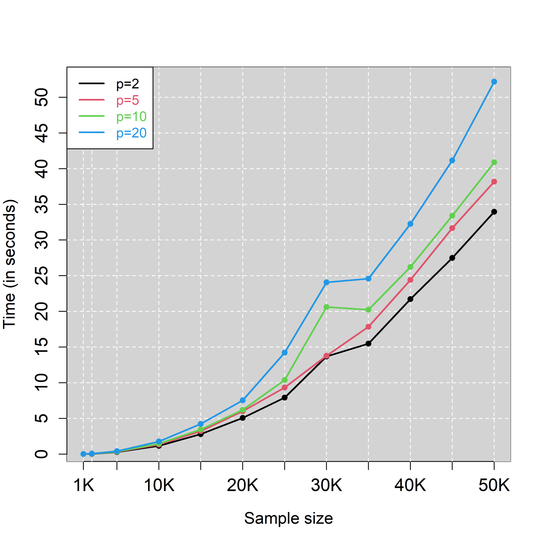
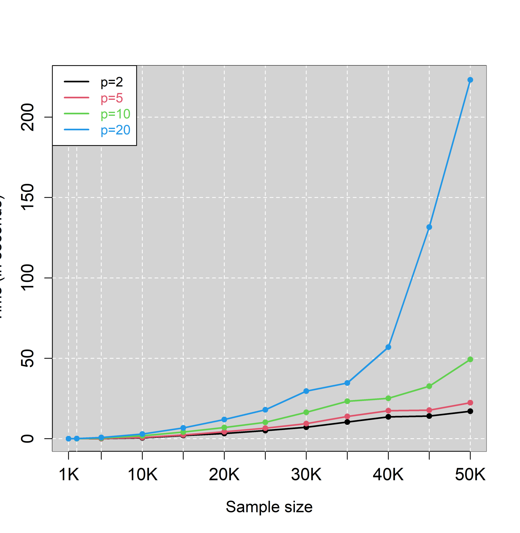
(a) Distance correlation	(b) Energy distance
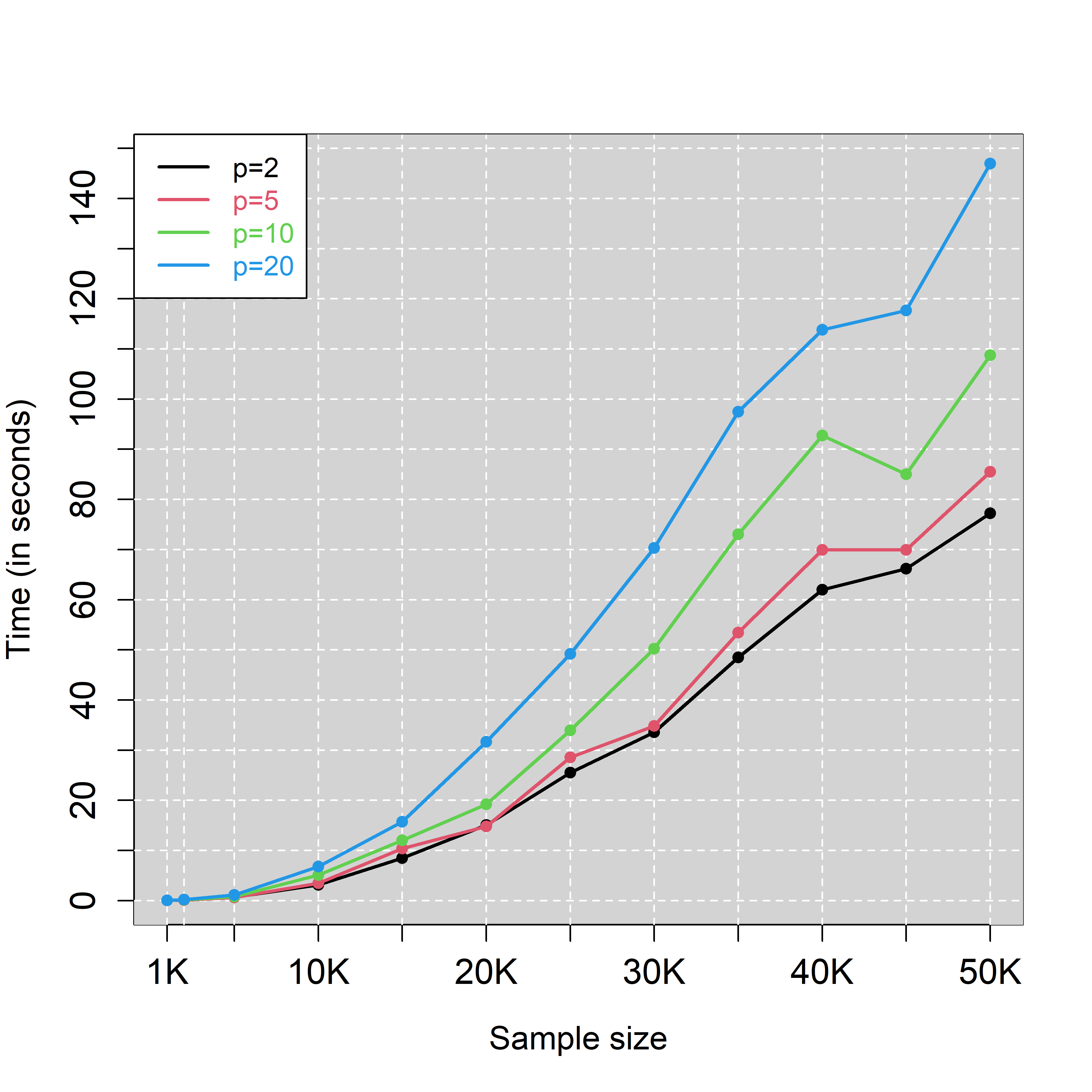
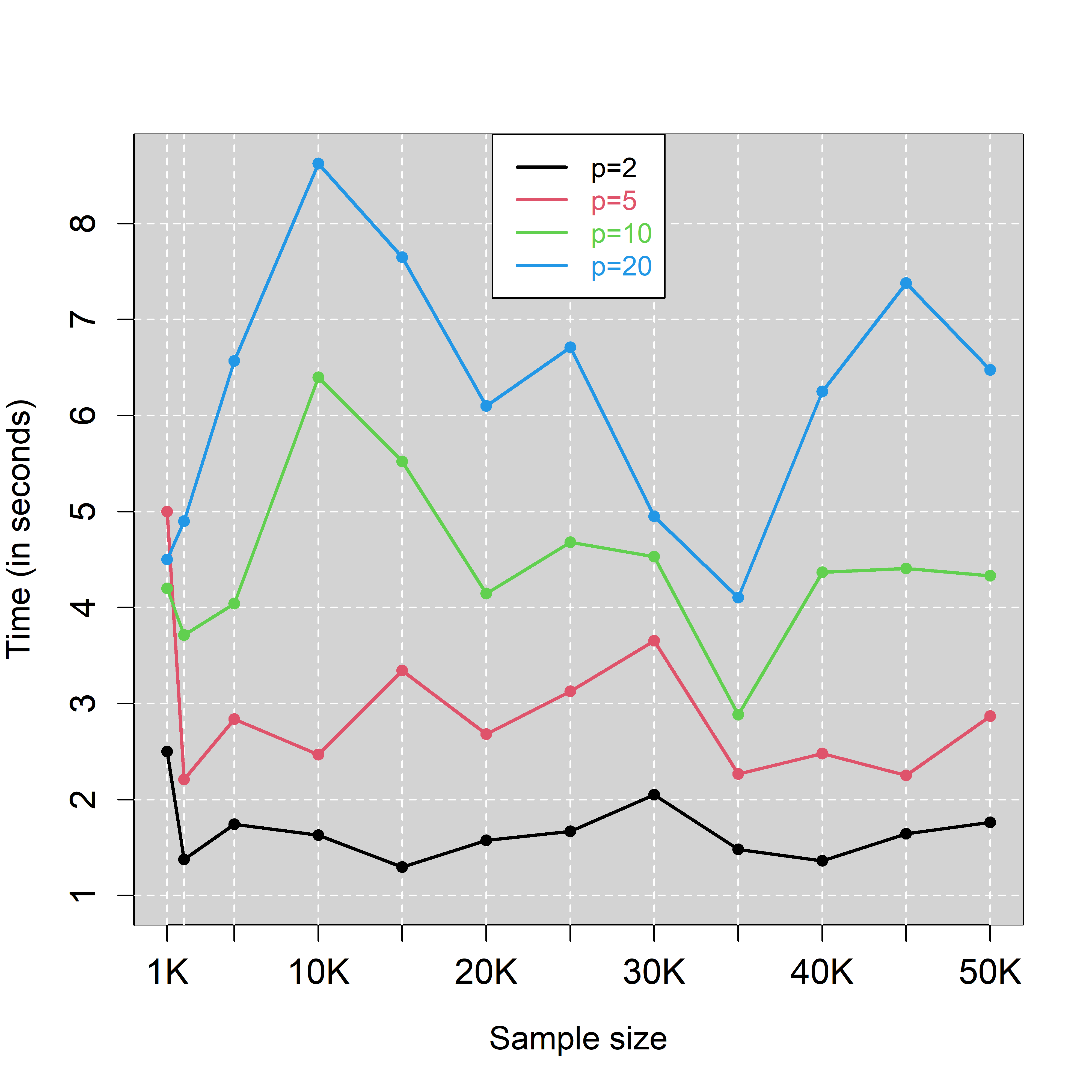
(c) Partial distance correlation	(d) Speed-up factor of Rfast::dcor()

Figure 1: Sample size versus running time for the Rfast implementations of (a) distance correlation and (b) energy distance, (c) partial distance correlation and (d) speed-up factor of Rfast::dcor() to dcortools::distcor().

Table 4: Running times (in seconds) of the energy, Rfast implementations of the equality of univariate distributions with $999$ permutations. Empty cells imply that the quantity could not be computed by the energy package implementation due to memory limitations.
^∗In the case of $n=15000$ the energy implementation required 516.082 seconds for only 4 permutations. Thus it would take more than 1 day to perform 999 permutations.

Sample size	energy	R
$n=1000$	5.068	0.138
$n=2000$	28.512	0.320
$n=5000$	178.040	0.782
$n=10000$	712.880	1.940
$n=15000$	516.082∗	3.240
$n=20000$	-	4.172
$n=25000$	-	4.734
$n=30000$	-	5.598
$n=35000$	-	7.186
$n=40000$	-	6.038
$n=45000$	-	6.706
$n=50000$	-	7.900

5 Conclusions

We showed a simple trick to alleviate the memory requirements and the computational cost associated with the energy distance, and the distance variance, covariance and correlation measures. Our next goal is to transfer the equality of univariate distributions testing code in C++. The same is true for the implementation of the partial distance correlation but in this case we must also reduce the number of calculations so as to make this function faster. We would also like to create more efficient functions of computing the permutation based p-value for more hypothesis testing procedures.

Appendix

The R version of the command dvar() to compute the distance variance for a vector

dvar <- function(x, bc = FALSE) {
  n <- length(x)
  i <- 1:n
  x <- Rfast::Sort(x)
  sxi <- cumsum(x)
  sxn <- sxi[n]
  ai <- (2 * i - n) * x + sxn - 2 * sxi
  #D <- Rfast::Dist(x, square = TRUE, result = "sum")
  D <- n * sum(x^2) - sxn^2
  if ( bc ) {
    a <- 2 * D / ( n * (n - 3) ) - 2 / ( n * (n - 2) * (n - 3) ) * sum(ai^2) +
         sum(ai)^2 / (n * (n - 1) * (n - 2) * (n - 3) )
  } else  a <- 2 * D/n^2 - 2/n^3 * sum(ai^2) + sum(ai)^2/n^4
  sqrt(a)
}

The R version of the command pdcor() to compute the partial distance correlation

pdcor <- function(x, y, z) {
  a1 <- Rfast::dcor(x, y, bc = TRUE)$dcor
  a2 <- Rfast::dcor(x, z, bc = TRUE)$dcor
  a3 <- Rfast::dcor(y, z, bc = TRUE)$dcor
  up <- a1 - a2 * a3
  down <- sqrt( 1 - a2^2 ) * sqrt( 1 - a3^2 )
  up / down
}

The R version of the command eqdist.etest() to test the equality of two univariate or multivariate distributions

eqdist.etest <- function(y, x, R = 999) {
  if ( !is.matrix(x) ) {
    ## univariate
    #dii is the sum of all pairwise distances of x
    ni <- length(x)
    i <- 1:ni
    x <- Rfast::Sort(x)
    sx <- sum(x)
    dii <- 2 * sum(i * x) - (ni + 1) * sx
    #djj is the sum of all pairwise distances of y
    nj <- length(y)
    j <- 1:nj
    y <- Rfast::Sort(y)
    sy <- sum(y)
    s <- sx + sy
    djj <- 2 * sum(j * y) - (nj + 1) * sy
    n <- ni + nj  ## total sample size
    z <- Rfast::Sort( c(x, y) )
    ##dij <- Rfast::dista(x, y, result = "sum")
    dtot <- 2 * sum( ( 1:n ) * z ) - (n + 1) * s
    dij <- dtot - dii - djj
    stat <- dij - nj * dii / ni - ni * djj / nj

    pstat <- numeric(R)
    for ( k in 1:R ) {
      id <- Rfast::Sort.int( Rfast2::Sample.int(n, ni) )
      xp <- z[id]
      sxp <- sum(xp)
      pdii <- 2 * sum(i * xp) - (ni + 1) * sxp
      yp <- z[-id]
      syp <- s - sxp
      pdjj <- 2 * sum(j * yp) - (nj + 1) * syp
      pdij <- dtot - pdii - pdjj
      pstat[k] <- pdij - nj * pdii / ni - ni * pdjj / nj
    }
    ## multivariate
  } else {
    nx <- dim(x)[1]  ;  ny <- dim(y)[1]
    n <- nx + ny
    stat <- Rfast::edist(x, y)
    z <- rbind(x, y)
    for ( k in 1:R ) {
      id <- Rfast2::Sample.int(n, nx)
      pstat[k] <- Rfast::edist(z[id, ], z[-id, ])
    }
  }
  ( sum( pstat >= stat ) + 1 ) / (R + 1)
}

References

- Edelmann and Fiedler, (2022) Edelmann, D. and Fiedler, J. (2022). dcortools: Providing Fast and Flexible Functions for Distance Correlation Analysis. R package version 0.1.6.
- Edelmann et al., (2019) Edelmann, D., Fokianos, K., and Pitsillou, M. (2019). An updated literature review of distance correlation and its applications to time series. International Statistical Review, 87(2):237–262.
- Hou et al., (2022) Hou, J., Ye, X., Feng, W., Zhang, Q., Han, Y., Liu, Y., Li, Y., and Wei, Y. (2022). Distance correlation application to gene co-expression network analysis. BMC bioinformatics, 23(1):81.
- Huo and Székely, (2016) Huo, X. and Székely, G. J. (2016). Fast computing for distance covariance. Technometrics, 58(4):435–447.
- Kasieczka and Shih, (2020) Kasieczka, G. and Shih, D. (2020). Robust jet classifiers through distance correlation. Physical review letters, 125(12):122001.
- Li et al., (2012) Li, R., Zhong, W., and Zhu, L. (2012). Feature screening via distance correlation learning. Journal of the American Statistical Association, 107(499):1129–1139.
- MacCarron et al., (2023) MacCarron, P., Mannion, S., and Platini, T. (2023). Correlation distances in social networks. Journal of Complex Networks, 11(3):cnad016.
- Papadakis et al., (2024) Papadakis, M., Tsagris, M., Dimitriadis, M., Fafalios, S., Fasiolo, M., Jacob, M., Borboudakis, G., Burkardt, J., Zou, C., Lakiotaki, K., and Chatzipantsiou, C. (2024). Rfast: A Collection of Efficient and Extremely Fast R Functions. R package version 2.1.3.
- Rizzo and Szekely, (2024) Rizzo, M. and Szekely, G. (2024). energy: E-Statistics: Multivariate Inference via the Energy of Data. R package version 1.7-12.
- Speed, (2011) Speed, T. (2011). A correlation for the 21st century. Science, 334(6062):1502–1503.
- Székely and Rizzo, (2009) Székely, G. J. and Rizzo, M. L. (2009). Brownian distance covariance. Annals of Applied Statistics, 3(4):1236–1265.
- Székely and Rizzo, (2023) Székely, G. J. and Rizzo, M. L. (2023). The energy of data and distance correlation. Chapman and Hall/CRC.
- Székely et al., (2007) Székely, G. J., Rizzo, M. L., and Bakirov, N. K. (2007). Measuring and testing dependence by correlation of distances. Annals of Statistics, 35(6):2769–2794.
- Ugwu et al., (2023) Ugwu, S., Miasnikof, P., and Lawryshyn, Y. (2023). Distance Correlation Market Graph: The Case of S&P500 Stocks. Mathematics, 11(18):3832.