Graph-based Retrieval Augmented Generation for Dynamic Few-shot Text Classification

Abstract.

Text classification is a fundamental task in natural language processing, pivotal to various applications such as query optimization, data integration, and schema matching. While neural network-based models, such as CNN and BERT, have demonstrated remarkable performance in text classification, their effectiveness heavily relies on abundant labeled training data. This dependency makes these models less effective in dynamic few-shot text classification, where labeled data is scarce, and target labels frequently evolve based on application needs. Recently, large language models (LLMs) have shown promise due to their extensive pretraining and contextual understanding. Current approaches provide LLMs with text inputs, candidate labels, and additional side information (e.g., descriptions) to predict text labels. However, their effectiveness is hindered by the increased input size and the noise introduced through side information processing. To address these limitations, we propose a graph-based online retrieval-augmented generation framework, namely GORAG, for dynamic few-shot text classification. GORAG constructs and maintains an adaptive information graph by extracting side information across all target texts, rather than treating each input independently. It employs a weighted edge mechanism to prioritize the importance and reliability of extracted information and dynamically retrieves relevant context using a minimum-cost spanning tree tailored for each text input. Empirical evaluations demonstrate that GORAG outperforms existing approaches by providing more comprehensive and accurate contextual information.

PVLDB Reference Format:
PVLDB, 14(1): XXX-XXX, 2020.
doi:XX.XX/XXX.XX

PVLDB Artifact Availability:
The source code, data, and/or other artifacts have been made available at ***.

1. Introduction

Text classification is a fundamental task that is connected to various other tasks, such as query optimization (Yu et al., 2023; Yu and Litchfield, 2020) data integration (Dong and Rekatsinas, 2018), and schema matching (Sahay et al., 2020; Zhang et al., 2024a). For example, in schema matching tasks, a text classifier can be trained to determine whether two schema attributes refer to the same concept based on their descriptions or metadata (Zhang et al., 2024a). In recent years, Neural Network (NN)-based models (Johnson and Zhang, 2015; Prieto et al., 2016; Liu et al., 2016; Dieng et al., 2017; Wang et al., 2017; Johnson and Zhang, 2017; Peters et al., 2018; Wang et al., 2018; Yang et al., 2019; Miao et al., 2021), such as CNN (Kim, 2014), Bert (Devlin, 2018) and RoBERTa (Liu, 2019), have demonstrated impressive performance on text classification tasks. However, the effectiveness of these NN-based approaches depend on abundant labeled training data, which requires significant time and human efforts (Meng et al., 2018). Consequently, these methods perform poorly with limited labeled text data (Xia et al., 2021), such as in few-shot text classification tasks (Wang et al., 2020; Aljehani et al., 2024).

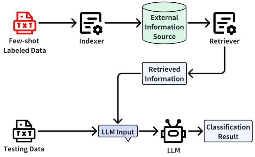
Figure 1. An illustration of the structural composition of current Reteieval Augmented Generation based few-shot text classification models, where the few-shot labeled training data is indexed as an external information source. During classification, the model retrieves side information from the external information source to provide additional context that aids the classification process.

Also, in real-world applications, such as Web Of Science (Kowsari et al., 2017) and IMDb (imd, [n.d.]), target labels for text often change based on the application’s requirements (Xia et al., 2021), leading to dynamic text classification. For instance, movie labels might initially be {Action, Thriller, Comedy}, but platforms may need to add more genres (e.g., Romantic and Comic) to extend the original labels. Therefore, it is important to classify text into these new categories. Consequently, how to develop methods to dynamically classify text with limited labeled data (i.e., dynamic few-shot text classification) remains a necessity and open problem.

Depending the technique for dynamic few-shot text classification task, current models can be categorized into three types, i.e., data augmentation-based (Meng et al., 2018; Meng et al., 2020; Xia et al., 2021), meta learning-based (Bansal et al., 2020; Zhang et al., 2023a), and large language model (LLM)-based approaches (Chen et al., 2023; Sarthi et al., 2024; Edge et al., 2024; Gutiérrez et al., 2024; Guo et al., 2024). Firstly, data augmentation-based models create additional training data by mixing the pairs of the few-shot labeled data and assign a mixed labels for these created data based on the labels of each pairs of data (Xia et al., 2021). Also, several data augmentation approaches create extra semantic related content based on the label names (Meng et al., 2018; Meng et al., 2020). However, due to the limited labeled data, the generated text data has very limited patterns. Consequently, the text classification models trained on these generated data are over-fitting on limited text data and are not generalizable (Liu et al., 2023). Also, meta-learning models (Bansal et al., 2020; Zhang et al., 2023a) train meta-learners on each base class to quickly adapt to new classes with minimal data. However, meta-learning still requires a substantial amount of labeled data for base classes.

Recently, large language models (Sun et al., 2021; Jiang et al., 2023; Touvron et al., 2023; Achiam et al., 2023; Yang et al., 2024), pretrained on extensive corpora, have achieved significant success due to their superior and comprehensive text understanding abilities. Several researchers (Chen et al., 2023; Sarthi et al., 2024) provide the text, candidate labels, and retrieve side information (e.g., descriptions of text and labels, or documents) for LLMs, and these LLMs output the labels of the text. Current work (Gao et al., 2023) demonstrates that this side information can provide context for the text and labels, enabling LLMs to comprehensively understand these inputs, which is a key component of the success of LLMs in text classification. However, the incorporation of side information can further increase the input size and noise (Chen et al., 2023), which impedes the efficiency and effectiveness of LLMs (Sarthi et al., 2024). As a result, compression-based retrieval-augmented generation (RAG) approaches (Edge et al., 2024; Gutiérrez et al., 2024; Guo et al., 2024) are proposed to construct graphs by extracting key information from the side information sources. These models then only retrieve the information (e.g., graph path or subgraphs) relevant to the target text as the side information for LLMs, reducing the length of inputs for LLMs.

However, existing compression-based RAG approaches (Edge et al., 2024; Guo et al., 2024; Gutiérrez et al., 2024) still have three limitations in the dynamic few-shot text classification task. Firstly, these approaches only extract information and build an information graph based on the side information of each text individually. In this way, they do not merge the information graphs of different text inputs into a single graph to obtain more comprehensive information for incoming target texts. Consequently, they fail to consider the correlation between side information of different text inputs, providing insufficient and incomplete context for LLMs. Secondly, existing approaches construct graphs by indexing extracted information linkages uniformly. They do not consider the varying importance and extraction confidence of each link, which may provide incorrect and unreliable context for LLMs. Thirdly, existing approaches select relevant information for each input text based on a globally predefined threshold. However, the optimal retrieval threshold can vary across different text samples, making the globally predefined threshold suboptimal for the entire dataset.

To address the aforementioned issues, we propose a novel Graph-based Online Retrieval Augmented Generation framework for dynamic few-shot text classification, called GORAG. In general, GORAG constructs and maintains an adaptive online information graph by extracting side information from all target texts, tailoring graph retrieval for each input. Firstly, GORAG extracts keywords from the text using the LLM and links these keywords with the text’s ground truth label to represent the relationship between keywords and labels. Then, GORAG employs an edge-weighting mechanism when indexing edges into the information graph, assigning edge weights based on the importance of the keywords and their relevance to the respective text’s label. Secondly, when retrieving information from the graph for each text, GORAG retrieves candidate labels by constructing a minimum-cost spanning tree of text keywords mapped to the graph. After retrieval, the candidate labels serve as a filtered subset of the original target labels, which are then used to create input for the LLM. Since the generated spanning tree is determined solely by the graph information and the extracted text keywords, GORAG achieves adaptive retrieval without relying on any human-defined retrieval thresholds.

We summarize the novel contributions as follows.

• We present a RAG framework for few-shot text classification tasks, namely GORAG. The GORAG framework consists of four stages: (1) Graph construction, where a graph is built with keywords from the training texts considering their correlation with the texts’ label; (2) Candidate label retrieval, where relevant labels are adaptively retrieved from the graph for label pre-filtering; (3) Prompt construction, where prompts are generated based on the filtered candidate labels and the testing texts; and (4) Online indexing, where the keywords of the un-labeled text are indexed to the constructed graph based on the prediction result.

• We develop a novel graph edge weighting mechanism based on the keyword nodes’ importance within the text corpus, which can be applied during both graph construction and online indexing. This mechanism enables our approach to effectively model the relevance between keywords and labels, thereby reducing the noise introduced to the graph.

• To avoid the need for human-selected thresholds during retrieval, we formulate the candidate label retrieval problem which akin to the NP-hard Steiner Tree problem. To solve this problem, we modified the Mehlhorn algorithm (Mehlhorn, 1988) which provides an efficient and effective solution to the problem to generate candidate types from the information graph.

In the rest of this paper, we first present prelimnary and related work in section 2, the pipeline of our model GORAG in section 3, our experiments in section 4 and the final conclusion in section 5.

2. Preliminary and Related Works

In this section, we first introduce the preliminaries of dynamic few-shot text classification in Section 2.1 and then discuss the existing approaches in Section 2.2. The important notations used in this paper are listed in Table 1.

2.1. Dynamic Few-shot Text Classification

Text classification (Kowsari et al., 2019; Minaee et al., 2021; Li et al., 2022) is a key task in real-world application that involves assigning predefined labels $y\in\mathcal{Y}$ to text $t=(w_{1},\cdots,w_{|t|})$ based on its words $w_{i}$. It is widely applied in areas like sentiment analysis (Kouadri et al., 2020; maamar2022sa),query optimization (Yu et al., 2023; Yu and Litchfield, 2020) data integration (Dong and Rekatsinas, 2018), and schema matching (Sahay et al., 2020; Zhang et al., 2024a). Traditional approaches rely on large labeled datasets (Devlin, 2018; Liu, 2019), which may not always be available. Recently, few-shot learning addresses this limitation by enabling models to classify text with only a small number of labeled examples per class (Meng et al., 2018; Meng et al., 2020). Dynamic classification (Parisi et al., 2019; Hanmo et al., 2024; Wang et al., 2024) introduces an additional challenge where new classes are introduced over multiple rounds, requiring the model to adapt to new classes while retaining knowledge of previously seen ones. Combining these aspects, Dynamic Few-Shot Text Classification (DFSTC) (Xia et al., 2021) allows the model to handle evolving classification tasks with minimal labeled data.

In DFSTC, the model is provided with multiple rounds of new class updates. Specifically, In each round $r$, a new set of classes $\mathcal{Y}_{new}^{r}$ is introduced and the labelled dataset for $\mathcal{Y}_{\text{new}}^{r}$ is denoted as $\mathcal{D}_{new}^{r}=\cup_{y_{i}\in\mathcal{Y}_{\text{new}}^{r}}\{t_{j},y_{i}\}_{j=1}^{k}$, where per class $y\in\mathcal{Y}_{\text{new}}^{r}$ only has $k$ labeled examples $\{t_{j},y_{i}\}_{j=1}^{k}$. Also, we denote candidate cumulative labels from the first round to the $r$-th round as $\mathcal{Y}^{r}=\bigcup_{i=1}^{r}\mathcal{Y}_{\text{new}}^{i}$. Formally, at the $r$-th round, given the candidate labels $\mathcal{Y}^{r}$ and all labeled data $\mathcal{D}^{r}=\cup_{i=1}^{r}\mathcal{D}_{new}^{i}$, the target of DFSTC task is to learn a function $f^{r}_{\theta}$, which can learn scores for all target labels $\mathbf{s}^{r}_{k}={f}^{r}_{\theta}(t,\mathcal{Y}^{r})\in[0,1]^{|\mathcal{Y}^{r}|}$ for the unseen text $t_{k}$. Then, we can get the predicted label $y^{r*}_{k}\in\mathcal{Y}^{r}$ for the unseen text $t_{k}$ as follows.

(1) $$y^{r*}_{k}=\arg\max_{y^{r}_{k}\in\mathcal{Y}^{r}}({f}_{\theta}(t,\mathcal{Y}^{r})[y^{r}_{k}])$$

DFSTC is valuable for its ability to learn from limited labeled data, adapt to evolving class distributions, and address real-world scenarios where categories and data evolve over time. For example, in Round 1, the model might be trained on classes like Sports, Politics, and Technology. In Round 2, new classes such as Health and Education are introduced. The model must now classify texts into all five classes while retaining its knowledge of earlier ones. For instance, given the text ”The new vaccine shows promising results,” the model should classify it as Health.

2.2. Dynamic Few-shot Text Classification Models

Current dynamic few-shot text classification models can be broadly categorized into two types: Meta learning-based models and Data Augmentation-based models, and Large Language Model (LLM)-based models.

2.2.1. Meta learning-based models

Meta learning-based models train a meta-learner on base classes $C_{b}$ and then adapt it to new classes in each round. For instance, LEOPARD (Bansal et al., 2020) use the meta-learner to generate model parameters to predict classes in each round. ConEntail (Zhang et al., 2023a) trains the meta-learner to classify texts based on their nested entailments with class label names at each round. However, these models require a sufficient amount of training data to train the meta-learner, which differs from our experimental setting and limits their generalization ability.

2.2.2. Data Augmentation-based models

Data Augmentation-based models generate additional data contrastively based on the few-shot labeled data to train the classifier. For example, Entailment (Xia et al., 2021) creates extra data samples, by concatenating texts with class label names. WeSTClass (Meng et al., 2018) trains a document generator to produce pseudo documents contrastively based on few-shot training data. LOTClass (Meng et al., 2020) uses a Pretrained Language Model (PLM) to generate words semantically correlated with the class label name to help with the classification. However, due to the limited labeled data, the generated text data of these models can have very limited patterns, which makes them prone to overfitting (Liu et al., 2023).

Table 1. Summary on Important Notations.

Notations	Meanings
$t$	Text.
$w$	The edge weight.
$r$	The round of label updation.
$y\in\mathcal{Y}^{r}$	The target label at round $r$.
$k$	The number of labeled data provided per target label.
$f^{r}_{\theta}$	The function that learn all target labels’ score for texts.
$\mathbf{s}^{r}_{k}$	The score for all target labels at round $r$.
$y^{r*}_{k}$	The predicted label for the text.
$\mathcal{G}^{r}(\mathcal{V},\mathcal{E})$	Information graph with node set $\mathcal{V}$ and edge set $\mathcal{E}.$
$\mathcal{Y}^{r}$, $\mathcal{Y}^{r}_{new}$	All target label and new target labels at round $r$.
$\mathcal{D}^{r}$, $\mathcal{D}^{r}_{new}$	The labeled text for all labels and new labels at round $r$.
$\mathcal{T}^{r}$, $\mathcal{T}_{new}^{r}$	The text of all labels and new labels at round $r$.
$\mathcal{T}_{test}^{r}$	The testing text for at round $r$.
$\mathcal{K}_{new}^{r}$	The extracted keyword set for new labels of round $r$.
$\mathcal{V}_{new}^{r}$	The set of new graph nodes to be added in round $r$.
$\mathcal{N}(\cdot)$	The neighbor set of a node in the information graph.
$p_{extract}$	The extraction instruction prompt.
$p_{gen}$	The generation instruction prompt.
$p_{classify}$	The classification instruction prompt.
$CS(\cdot)$	The correlation score between keywords and labels.
$w^{r}_{v,y}$	The weight of edge $e_{v,y}$ in round $r$.
$P_{u,v}$	The shortest path between node $u$ and node $v$.
$\mathcal{V}_{exist}$	The keywords that exist in graph.
$\mathcal{V}_{notexist}$	The keywords do not exist in graph.
$\mathcal{E}_{oi}^{t}$	Edges added based on text $t$.

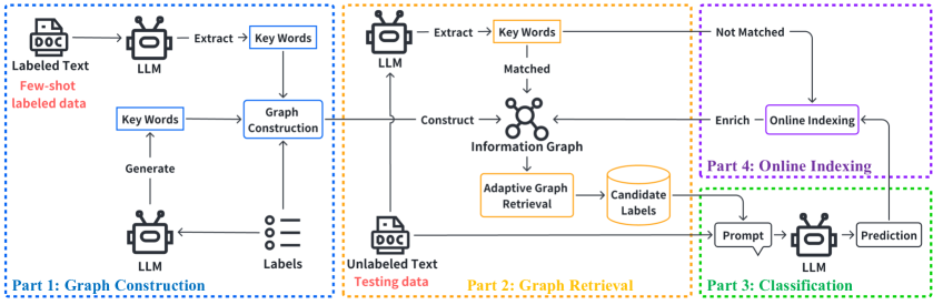
Figure 2. An overview of the GORAG model is as follows. In Part 1, GORAG constructs a graph based on keywords extracted from the few-shot training data, taking into account the keyword extraction confidence and relatedness to the target labels. In Part 2, GORAG performs adaptive graph retrieval and utilizes the retrieved graph information to filter the target labels. In Part 3, GORAG carry out classification with the testing texts and the candidate labels retrieved from the information graph. In Part 4, GORAG applies online indexing to update the graph with newly extracted nodes from testing texts through online indexing.

2.2.3. LLM-based models

Recently, Large Language Model (LLM)-based models have undergone rapid development (Fernandez et al., 2023; Amer-Yahia et al., 2023; Zhang et al., 2024b; Miao et al., 2024) and have been successfully adapted to various tasks, including data discovery (Arora et al., 2023; Dong et al., 2023; Kayali et al., 2024), entity or schema matching (Zhang et al., 2023b; Tu et al., 2023; Fan et al., 2024; Du et al., 2024), and natural language to SQL conversion (Li et al., 2024; Ren et al., 2024; Trummer, 2022; Gu et al., 2023). Notably, LLMs are inherently capable of inference without fine-tuning (Sun et al., 2021; Jiang et al., 2023; Touvron et al., 2023; Achiam et al., 2023; Yang et al., 2024), making them originally suitable for dynamic text classification tasks. However, the lack of fine-tuning can lead LLMs to generate incorrect answers, as they lack task-specific knowledge, these incorrect answers are often referred to as hallucinations (Zhang et al., 2023c). To mitigate hallucinations, researchers have provided LLMs with side information for classification, namely long context RAG models. For example, Propositionizer (Chen et al., 2023) applies a fine-tuned LLM to convert side information into atomic expressions, to facilitate fine-grained information retrieval. RAPTOR (Sarthi et al., 2024) clusters side information and then generate summaries for each cluster, to help with the model prediction. However, the retrieved contents from these models remain unstructured and can be lengthy, which impedes the efficiency and effectiveness of LLMs, leading to lost-in-the-middle issue (Liu et al., 2024).

To address this, compression-based RAG models were proposed, these models try to compress side information to reduce the input length. Based on how they compress model inputs, these models can be classified into prompt compressor models, and graph-based RAG models. On the one hand, prompt compressor models, such as LLMLingua2 (Pan et al., 2024), apply LLM’s generation perplexity to filter out un-important tokens in the model input. Based on LLMLingua2, LongLLMLingua (Jiang et al., 2024) further considers the instruction to the model when compression, make the model instruction-aware. On the other hand, graph-based RAG models index side informations into a graph, and retrieve graph components or summaries, which are shorter than long contexts thet traditional RAG models retrieved. For instance, GraphRAG (Edge et al., 2024) constructs a graph and aggregates nodes into graph communities, then generate community summaries to help the LLM prediction. However, GraphRAG requires re-creating the community after each graph index, which incurs significant computational overhead.

To address this limitation of GraphRAG, two alternative models, HippoRAG (Gutiérrez et al., 2024) and LightRAG (Guo et al., 2024), have been proposed, which skip the formulation of communities and directly retrieve nodes or pathes from graphs. HippoRAG (Gutiérrez et al., 2024) retrieve nodes whose retrieval score is above a human defined threshold. However, the optimal retrieval threshold can vary across different data samples, and a globally fixed threshold selected by human may be suboptimal for the entire dataset. To address this issue, LightRAG (Guo et al., 2024) calculates the embedding similarity of text extracted entities with graph nodes, to achieve a one-to-one mapping and retrieve all triples involved these graph nodes.

3. Methdology

To address the aforementioned issues, we propose GORAG, a novel approach that achieves adaptive retrieval by extracting valuable side information from a minimum-cost spanning tree generated on the constructed graph. Specifically, GORAG takes into account each keyword’s with in the training and texting text corpus and relatedness to the class label by assigning different costs to edges on the constructed graph, allowing for more informed retrieval decisions. Moreover, GORAG incorporates an online indexing mechanism, which enables the model to index valuable information extracted from the testing texts to the constructed graph in real-time, thereby enhancing its ability to make accurate predictions in the future.

3.1. Framework Overview

As illustrated in Figure 2, our model consists of four primary components, i.e., Graph Construction, Graph Retrieval, Classification, and Online Indexing.

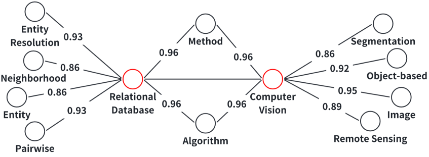
Figure 3. An example of the constructed information graph from WOS dataset, where red nodes denote the label node and black nodes denote the keyword node. In this subgraph, node Entity and node Neighborhood are considered most related to the label Relational Database, the edge between them with the label have the lowest cost assigned by our edge weighting mechanism.

Part 1: Graph Construction Graph construction proposes is to construct or update the information graph $\mathcal{G}^{r}_{new}(\mathcal{V}^{r}_{new},\mathcal{E}^{r}_{new},\mathcal{W}^{r}_{new})$ at round $r$ based on the labeled data $\mathcal{D}_{new}^{r}=\cup_{y_{i}\in\mathcal{Y}_{\text{new}}^{r}}\{t_{j},y_{i}\}_{j=1}^{k}$ for at the $r$-th round. A small subgraph of the information graph created on WOS dataset is shown in Figure 3, graph formed like this will be used to provide retrieved-augmented information as context for unseen text, enabling LLMs to better understand the unseen text and accurately predict its labels. Specifically, under each new data $\mathcal{D}_{new}^{r}$ at the $r$-th round, we first extract the new keywords $\mathcal{K}_{new}^{r}\in\{t_{j}\}_{j=1}^{|\mathcal{D}_{new}^{r}|}$ from the few-shot training texts $\mathcal{T}^{r}_{new}=\{t_{j}\}_{j=1}^{|\mathcal{D}_{new}^{r}|}$. Then, we will then assign an edge $e^{r}_{v,y}\in\mathcal{E}^{r}_{new}$ between each keyword $v\in\mathcal{K}_{new}^{r}$ and each label $y\in\mathcal{Y}^{r}_{new}$. We then compute the weight $w^{r}_{v,y}\in\mathcal{W}^{r}_{new}$ for each edge $e^{r}_{v,y}\in\mathcal{E}^{r}_{new}$ based on the keyword’s importance with in the text corpus and relatedness to the label $y$. We then can merge all graphs $\mathcal{G}^{r}_{new}(\mathcal{V}^{r}_{new},\mathcal{E}^{r}_{new},\mathcal{W}^{r}_{new})$ at each each round $r$ as the full graph $\mathcal{G}^{r}(\mathcal{V}^{r},\mathcal{E}^{r},\mathcal{W}^{r})$. More details can refer to Section 3.2.

Part 2: Graph Retrieval The Graph Retrieval process maps the extracted keyword nodes $\mathcal{V}^{t}$ from the unlabeled text $t$ to the constructed information graph $\mathcal{G}^{r}$ and generates a minimum-cost spanning tree on $\mathcal{G}^{r}$ that includes all these keywords. From this minimum-cost spanning tree, the candidate label set $\hat{\mathcal{Y}}_{t}^{r}$ is obtained, which is a reduced subset of the original target label set $\mathcal{Y}^{r}$. For more details, please refer to Section 3.3.

Part 3: Classification After retrieving the graph and obtaining the candidate types $\hat{\mathcal{Y}}_{t}^{r}$ for the text $t$ at round $r$, the classification procedure involves performing the final classification based on a large language model. This process utilizes the text $t$, the candidate labels $\hat{\mathcal{Y}}_{t}^{r}$ retrieved from the information graph $\mathcal{G}^{r}$, and descriptions $\mathcal{K}_{y_{i}}$ associated with each candidate label $y_{i}\in\hat{\mathcal{Y}}_{t}^{r}$. For more details, please refer to Section 3.4.1.

Part 4: Online Indexing The online indexing procedure dynamically indexes keywords, denoted as $\mathcal{V}_{\text{notexist}}^{t}$, which extracted from the testing text $t$ but are not in the existing graph $\mathcal{G}^{r}$. We then integrate these keywords into the graph to further enrich its structure, with weights assigned based on their importance within the text corpus and their relatedness to the predicted label $y^{*}_{t}$ for the testing text $t$. This process enhances the model’s ability to make more accurate predictions in the future. For more details, please refer to Section 3.4.2.

3.2. Part 1: Graph Construction

In this subsection, we would introduce the graph construction procedure of GORAG. To generate the information graph $\mathcal{G}^{r}(\mathcal{V}^{r},\mathcal{E}^{r},\mathcal{W}^{r})$ for each the $r$-th round, GORAG applies multiple instructions to the LLM for creating the graph node set $\mathcal{V}^{r}$ and the edges $e^{r}_{v,y}\in\mathcal{E}^{r}$ between keyword node $v$ and label node $y$. Also, we will assign weight $w^{r}_{v,y}\in\mathcal{W}^{r}$ for each each edge $e(v,y)$. The pseudo code of the graph construction algorithm is shown in Algorithm 1.

Algorithm 1 Graph Construction Algorithm of GORAG at the $r$-th round

0: $\mathcal{D}_{new}^{r}$: Training text set at the $r$-th round and the provided label $y_{i}\in\mathcal{Y}_{new}^{r}$ for each training text $t_{j}$; $p_{extraction},\ p_{gen}$: The extraction and description generation instruction prompt; $\mathcal{G}^{r-1}$: Information graph of the previous round $r-1$.

0: $\mathcal{G}^{r}$: Constructed information graph at the $r$-th round.

1: Let $\mathcal{V}_{text}^{r}=\emptyset$, $\mathcal{V}_{label}^{r}=\emptyset$, $\mathcal{E}_{new}^{r}=\emptyset$

2: for each text $t\in\mathcal{T}_{new}^{r}$ do

3:  $\mathcal{V}_{text}^{r}=\mathcal{V}_{text}^{r}\cup LLM(p_{extract},t)\cup y_{t}$

4: end for

5: if label names are available then

6:  for each label $y_{i}\in\mathcal{Y}_{new}^{r}$ do

7:   Get label description $\mathcal{K}_{y_{i}}=LLM(p_{gen},\mathcal{D}^{r})$.

8:   $\mathcal{V}_{label}^{r}=LLM(p_{extract},\mathcal{K}_{y_{i}})\cup\mathcal{V}_{label}^{r}$

9:  end for

10: end if

11: Let $\mathcal{V}_{new}^{r}=\mathcal{V}_{text}^{r}\cup\mathcal{Y}^{r}_{new}\cup\mathcal{V}_{label}^{r}$ be the new node set at the $r$-th round.

12: for each node $v\in\mathcal{V}_{new}^{r}$ do

13:  $\mathcal{E}_{new}^{r}=\mathcal{E}_{new}^{r}\cup e_{v,y_{i}}$

14:  $\mathcal{W}_{new}^{r}=\mathcal{W}_{new}^{r}\cup w_{v,y_{i}}^{r}$

15: end for

16: Let $\mathcal{G}^{r}_{new}=(\mathcal{V}_{new}^{r},\mathcal{E}_{new}^{r})$ be the newly constructed graph for at the $r$-th round.

17: Let $\mathcal{G}^{r}=Merge(\mathcal{G}^{r}_{new},\mathcal{G}^{r-1})$ be the final constructed graph at the $r$-th round.

18: return  $\mathcal{G}^{r}$

At each $r$-th round, given the labeled training text $\mathcal{D}_{new}^{r}=\cup_{y_{i}\in\mathcal{Y}_{\text{new}}^{r}}\{t_{j},y_{i}\}_{j=1}^{k}$, GORAG first extracts text keywords $\mathcal{K}^{r}_{new}$ from the text $\mathcal{T}^{r}_{new}=\cup_{y_{i}\in\mathcal{Y}_{\text{new}}^{r}}\{t_{j}\}_{j=1}^{k}$ to serve as graph nodes. Specifically, we use the LLM model with an extraction instruction prompt $p_{extract}$, such as $p_{extract}=$“Please extract some keywords from the following passage”. Then, we can get all text keywords $\mathcal{K}^{r}_{new}$ based on texts $\mathcal{T}^{r}_{new}$ as follows.

(2) $$\mathcal{K}^{r}_{new}=\bigcup_{t\in\mathcal{T}^{r}_{new}}LLM(p_{extract},t).$$

Also, by incorporating the new candidate labels $\mathcal{Y}^{r}_{new}$ at the $r$-th round, the graph node set $\mathcal{V}^{r}_{new}$ at the $r$-th round can be obtained as follows.

(3) $$\mathcal{V}_{new}^{r}=\mathcal{K}_{new}^{r}\cup\mathcal{Y}_{new}^{r}.$$

Then, GORAG links each keyword node $v\in\mathcal{K}_{{new}}^{r}$ to its corresponding label node $y\in\mathcal{Y}_{{new}}^{r}$, indicating that the keyword $v$ appears in texts associated with the label $y$.

We discuss how to compute the weight between each keyword node $v\in\mathcal{K}_{{new}}^{r}$ and each label $y\in\mathcal{Y}_{{new}}^{r}$. Considering the keywords $\mathcal{K}_{new}^{r}$ from the labeled text are not uniformly related to the text’s label $\mathcal{Y}_{new}^{r}$, we apply an edge weighting mechanism to assign a weight $w_{v,y}$ to each keyword-label link. This weight can be regarded as the correlation between keyword and each label. Firstly, we apply the $l_{2}$ normalized TF-IDF score (Sammut and Webb, 2010) to measure the importance and relatedness of a particular keyword $v\in\mathcal{K}_{new}^{r}$ and label $y\in\mathcal{Y}_{new}^{r}$ of the text $t\in\mathcal{T}^{r}$, where $\mathcal{T}^{r}=\cup_{i=1}^{r}\mathcal{T}_{new}^{i}$ denotes texts seen so far. Formally, given a keyword node $v\in\mathcal{K}_{new}^{r}$ and one text $t\in\mathcal{T}^{r}$, the correlation score $CS(v,t)$ between $v$ and $t$ is defined as follows.

(4) $$CS(v,t)=\frac{count(v,t)}{|t|}\times log\frac{|\mathcal{T}^{r}|}{1+|t_{j}:v\in t_{j},\ t_{j}\in\mathcal{T}^{r}|},$$

where $count(v,t)$ is the number of times that the term $v$ appears in the text $t$, and $|t_{j}:v\in t_{j},\ t_{j}\in\mathcal{T}^{r}|$ denotes the number of texts in the corpus $\mathcal{T}^{r}$ that contain the keyword $v$.

As the keyword $v$ can be extracted from multiple text source and from different rounds, the final edge weight $w_{v,y}^{r}$ of edge $e_{v,y}$ at the $r$-th round is calculated an the average of weights from all these texts. Formally, given the keyword $v\in\mathcal{K}_{new}^{r}$, label $y\in\mathcal{Y}_{new}^{r}$, and the texts $\mathcal{T}^{r,y}=\{t_{i}\}_{i=1}^{|\mathcal{T}^{r,y}|}$ consisting of texts $t_{i}$ associated with label $y$, the weight $w_{v,y}^{r}$ between $v$ and $y$ at the $r$-th round can be computed as follows:

(5) $$w_{v,y}^{r}=\frac{\sum_{t_{j}\in\mathcal{T}^{r,y,v}}1-CS(v,t_{j})}{|\mathcal{T}^{r,y,v}|},$$

where $\mathcal{T}^{r,y,v}=\{t_{j}|v\in t_{j}\land t_{j}\in\mathcal{T}^{r,y}\}$ is the text associated with label $y$ and containing the keyword $v$. We denote the generated graph for $\mathcal{K}_{new}^{r}$ and $\mathcal{Y}_{new}^{r}$ at the $r$-th round as $\mathcal{G}^{r}_{new}(\mathcal{V}_{new}^{r},\mathcal{E}_{new}^{r},\mathcal{W}_{new}^{r})$, where the node $\mathcal{V}^{r}_{new}=\mathcal{K}_{new}^{r}\cup\mathcal{Y}_{new}^{r}$ and edge $e^{r}_{v,y}\in\mathcal{E}_{new}^{r}$ is associated with the weight $w^{r}_{v,y}\in\mathcal{W}_{new}^{r}$.

We then discuss how to merge $\mathcal{G}^{r}_{new}$ into the graph from previous rounds $\mathcal{G}^{r-1}(\mathcal{V}^{r-1},\mathcal{E}^{r-1})$ to form the full graph $\mathcal{G}^{r}(\mathcal{V}^{r},\mathcal{E}^{r})$ as follows.

(6) $$\mathcal{G}^{r}=Merge(\mathcal{G}^{r}_{new},\mathcal{G}^{r-1}),$$

where $\mathcal{V}^{r}=\mathcal{V}^{r}_{new}\cup\mathcal{V}^{r-1}$, $\mathcal{E}^{r}=\mathcal{E}^{r}_{new}\cup\mathcal{E}^{r-1}$, and $\mathcal{W}^{r}=\mathcal{W}^{r}_{new}\cup\mathcal{W}^{r-1}$. Particularly, $\mathcal{G}^{0}=\emptyset$ and $\ r\geq 1$, Also, to guarantee the graph connectivity of the resulting graph, we add new edges between every newly added label node $y_{n}\in\mathcal{Y}_{new}^{r}$ and each old label node $y_{o}\in\mathcal{Y}^{r-1}$, the edge weight $w_{v,y}^{r}$ of edge $e_{y_{n},y_{o}}$ at round $r$ is calculated with the average weight of all edges that link keywords with label node $y_{n}$ or $y_{o}$, respectively:

(7) $$w_{y_{n},y_{o}}^{r}=\frac{AvgWei(y_{n},\mathcal{G}^{r})+AvgWei(y_{o},\mathcal{G}^{r-1})}{2}$$

(8) $$AvgWei(y,\mathcal{G}^{r})=\frac{\sum_{v\in\mathcal{M}_{y}^{r}}w_{v,y}^{r}}{2\times|\mathcal{M}_{y}^{r}|},$$

where $\mathcal{N}^{r}(y)$ denote the neighbor node set of label node $y$ in graph $\mathcal{G}^{r}$. Also, $\mathcal{M}_{y}^{r}=\{v\ |\ v\in\mathcal{N}^{r}(y)\ \land\ v\notin\mathcal{Y}^{r}\}$ denotes all neighbor nodes of label node $y$ that represent keywords, but not labels at the $r$-th round. After merge, the graph $\mathcal{G}^{r}$ would be used for future retrieval, and be further updated by GORAG’s online indexing mechanism later in Section 3.3.

Algorithm 2 Adaptive Candidate Type Generation Algorithm

0: $\mathcal{G}^{r}(\mathcal{V}^{r},\mathcal{E}^{r},\mathcal{W}^{r})$: The constructed information graph; $\mathcal{V}_{exist}^{t}\subseteq\mathcal{V}^{r}$: A set of keyword nodes extracted from text $t$ and can be mapped to graph $\mathcal{G}$; $\mathcal{Y}^{r}$: The target label set at the $r$-th round.

0: $\hat{\mathcal{Y}}^{r}_{t}$: The candidate type retrieved for text $t$.

1: Compute a minimum spanning tree $MST$ of the graph $\mathcal{G}$.

2: Let $\mathcal{V}_{term}=\mathcal{V}_{exist}^{t}\cap\mathcal{V}(MST)$ be the terminal nodes in $MST$

3: Construct a weighted auxiliary graph $H$: $\mathcal{V}(H)=\mathcal{V}_{term}$

4: for each pair of terminals $u,v\in\mathcal{V}_{term}$ do

5:  Find the shortest path $P_{uv}$ in $MST$ from $u$ to $v$

6:  Let $w^{H}_{u,v}=\sum_{e\in P_{uv}}w_{e}$

7: end for

8: Compute a minimum spanning tree $MST^{\prime}$ of the auxiliary graph $H$

9: Let $ST=\emptyset$

10: for each edge $e_{u,v}\in MST^{\prime}$ do

11:  Add the shortest path $P_{uv}$ in $MST$ to $ST$

12: end for

13: Let $\hat{\mathcal{Y}}^{r}_{t}=ST\cap\mathcal{Y}^{r}$

14: return  $\hat{\mathcal{Y}}^{r}_{t}$

3.3. Part 2: Graph Retrieval

In this subsection, we would introduce the graph retrieval procedure of GORAG. With the graph constructed in Part 1, GORAG is able to carry out adaptive reteieval algorithm with the keywords extracted from the testing texts.

To begin with, GORAG extract keywords $\mathcal{V}_{test}^{t}$ for each testing text $t\in T_{test}$ in the same manner with Equation (2), then, $\mathcal{V}_{test}^{t}$ would be splitted into two subsets:

(9) $$\mathcal{V}_{exist}^{t}\cup\mathcal{V}_{notexist}^{t}=\mathcal{V}_{test}^{t},\ \mathcal{V}_{exist}^{t}\cap\mathcal{V}_{notexist}^{t}=\emptyset,$$

where $\mathcal{V}_{exist}^{t}$ and $\mathcal{V}_{notexist}^{t}$ denotes the keywords in $\mathcal{V}_{test}^{t}$ that already exist and not yet exist in $\mathcal{G}^{r}$ at the current the $r$-th round respectively. Later, $\mathcal{V}_{exist}^{t}$ would be applied for achieving adaptive retrieval, and $\mathcal{V}_{notexist}^{t}$ would be applied for online indexing to further enrich the constructed graph (Further illustrated in Section 3.4).

To achieve the adaptive retrieval, GORAG try to find the minimum cost spanning tree that contain all keyword nodes within $\mathcal{V}_{exist}^{t}$. The intuition behind this approach is that a minimum cost spanning tree (MST) spans the entire graph to cover all given nodes with the smallest possible spanning cost. Consequently, nodes within the generated MST can be considered important for demonstrating the features of the given node set. The generation of an MST is a classical combinatorial optimization problem with an optimal solution determined solely by the set of given nodes. By generating the MST, we eliminate the need for any human-defined thresholds, relying instead on the LLM-extracted keywords to form the spanning tree.

Definition 3.1 (Adaptive Candidate Type Generation Problem).

Given an undirected weighted information graph $\mathcal{G}^{r}(\mathcal{V}^{r},\mathcal{E}^{r},\mathcal{W}^{r})$, a set of keywords $\mathcal{V}_{exist}^{t}$ extracted from text $t$ that can be mapped to nodes in $\mathcal{V}^{r}$, and the target label set $\mathcal{Y}^{r}$ at the $r$-th round, our target is to find a set of labels nodes ${\mathcal{Y}}^{r}_{t}\in{\mathcal{Y}}^{r}$. Firstly, we identify a subgraph $\mathcal{G}^{r}_{t}(\mathcal{V}^{r}_{t},\mathcal{E}^{r}_{t},\mathcal{W}^{r}_{t})$ of $\mathcal{G}^{r}$ by minimizing the edge weight sum as follows.

(10) $$\min_{e^{r}_{u.v}\in\mathcal{E}^{r}_{t}}w^{r}_{u,v}$$

(11) $$s.t.\ v\in\mathcal{V}^{r}_{t},\forall v\in\mathcal{V}_{exist}^{t}$$

Then, since the subgraph nodes $\mathcal{V}^{r}_{t}$ contains both keyword nodes and labels, we take the label nodes ${\mathcal{Y}}^{r}_{t}\in\mathcal{V}^{r}_{t}$ as our target candidate nodes for the text $t$.

Theorem 3.2.

The Adaptive Candidate Type Generation problem is NP-hard.

Proof.

To demonstrate that the Adaptive Candidate Type Generation problem is NP-hard, we provide a simple reduction of our problem from the Steiner Tree problem. Since the Steiner Tree problem is already proven to be NP-hard (Su et al., 2020), we show that there is a solution for the Steiner Tree problem if and only if there is a solution for our problem. Firstly, given a solution $S$ for our problem, we can construct a Steiner Tree by generating a minimum spanning tree for all nodes in $S$ on graph $\mathcal{G}^{r}$ then connecting all nodes from $\mathcal{V}_{exist}^{t}$ to their closest neighbor nodes in $S$. Secondly, any Steiner Tree $ST$ that contains any node $y\in\mathcal{V}^{r}_{t}$ is also a solution of our problem with $|\{y\in\mathcal{V}^{r}_{t}\}|$ nodes. Thus, we prove that the adaptive candidate type generation problem is NP-hard. ∎

Since this problem is the NP-hard, it is infeasible to obtain the optimal result in polynomial time. Therefore, to solve this problem, we propose a greedy algorithm, which generates the candidate type set ${\mathcal{Y}}^{r}_{t}\subseteq\mathcal{Y}^{r}$ for text $t$ at the $r$-th round. The detail of our algorithm is shown in Algorithm 2. Firstly, we calculate the shortest path between each keyword node $v$ in $\mathcal{V}_{exist}^{t}$ to all other nodes in $\mathcal{G}^{r}$ by calculating the minimum spanning tree $MST$ of $\mathcal{G}^{r}$ (line 1-2). Here, the keyword nodes $v$ in $\mathcal{V}_{exist}^{t}$ are served as terminal nodes that determins the final genrated candidate types w.r.t. to the information graph $\mathcal{G}^{r}$ . Secondly, we create a new auxiliary graph $H$ where the edges represent the shortest paths between the closest terminal nodes (line 3-7). Thirdly, we construct the minimum spanning tree $MST^{\prime}$ of the auxiliary graph $H$ (line 9), and then we add the shortest paths between each two nodes in $MST^{\prime}$ to the Steiner Tree $ST$ (line 10-12). Lastly our candidate types $\hat{\mathcal{Y}}^{r}_{t}$ for text $t$ are calculated as the interselect of $ST$ and all target labels $\mathcal{Y}^{r}$ at round $r$: $ST\cap\mathcal{Y}^{r}$ (line 13).

Note that in GORAG’s retrieval algorithm, the minimum-cost spanning tree is generated solely based on the constructed graph and the keywords extracted from the text. This approach eliminates the need for any manually defined retrieval thresholds, enabling GORAG to perform fully adaptive and context-driven retrieval.

3.4. Part 3: Classification and Online Indexing

In this subsection, we introduce GORAG’s two main components, i.e., classification and online indexing. For classification, GORAG utilizes an LLM to predict the class label for each unseen test text by retrieving adaptive demonstrations. For online indexing, GORAG dynamically updates the graph $\mathcal{G}^{r}$ by incorporating unseen keywords from the test text $t$ as new nodes and connecting them to the predicted label $y^{*}_{t}$ with weighted edges. This iterative process enriches the graph and enhances the framework’s ability to make accurate predictions in the future.

3.4.1. Classification

In this part, we introduce how GORAG performs text classification based a large language model. Specifically, for each unlabeled text $t$, GORAG predicts its class label $y^{*}$ by constructing an input $c_{t}$ for the LLM, which captures contextual and structural information about the text and its candidate labels. Specifically, given each unlableed text $t$, we will use LLM to predict its class label $y^{*}$. We first generate the LLM input $c_{t}$ as follows.

(12) $$c_{t}=Concat(t,\mathcal{K}^{t},\hat{\mathcal{Y}}^{r}_{t},\mathcal{K}_{\hat{\mathcal{Y}}^{r}_{t}}),$$

which is the text concatenation of the extracted keywords $\mathcal{K}^{t}$ from the text $t$, the candidate labels $\hat{\mathcal{Y}}^{r}_{t}$ obtained by Algorithm 2. Also, $\mathcal{K}_{\hat{\mathcal{Y}}^{r}_{t}}=\{\mathcal{K}_{y_{i}}\}_{i=1}^{|\hat{\mathcal{Y}}^{r}_{t}|}$ and $\mathcal{K}_{y_{i}}$ is the representative keywords of each label $y_{i}\in\hat{\mathcal{Y}}^{r}_{t}$.

(13) $$\mathcal{K}_{y_{i}}=LLM(p_{gen},\mathcal{D}^{r}),$$

and a classification instruction prompt $p_{classify}$.

(14) $$y^{*}_{t}=LLM(p_{classify},c_{t}),$$

As a result, the LLM would try to select the best-suited label $y^{*}_{t}\in\mathcal{Y}^{t}$ to annotate the text $t$.

3.4.2. Online indexing

To fully leverage the text-extracted keywords, GORAG utilizes an online indexing mechanism to incrementally update keywords that do not yet exist in the information graph $\mathcal{G}^{r}$ at the $r$-th round to the information graph $\mathcal{G}^{r}$ based on the text $t$’s predicted label $y^{*}_{t}$. To be specific, each keyword node $v\in\mathcal{V}_{notexist}^{t}$ would be directed added to the original graph’s node set $\mathcal{V}^{r}$ and be assigned with an edge $e_{v,y}$ connect it with the predicted label $y$:

(15) $$\mathcal{V}^{r}=\mathcal{V}^{r}\cup\mathcal{V}_{notexist}^{t},\ \mathcal{E}^{r}=\mathcal{E}^{r}\cup\mathcal{E}_{oi}^{t},$$

where $\mathcal{E}_{oi}^{t}=\{e_{v,y_{t}}|v\in\mathcal{V}_{notexist}^{t}\}$ denotes the set of all newly assigned edges $e_{v,y}$ between keyword node $v$ and its predicted label $y_{t}^{*}$, for these newly assigned edges, their weight is calculated with the edge weighting mechanism illustrated in Equation (5).

Table 2. Statistics of the WOS and Reuters dataset.

Dataset	Avg. Text Token	R1		R2		R3		R4		Total
		Testing data	Label #	Testing data	Label #	Testing data	Label #	Testing data	Label #	Testing data
WOS (Kowsari et al., 2017)	200	2,417	32	2,842	53	2,251	30	1,886	18	9,396
Reuters (Bao et al., 2020)	168	80	8	80	8	80	8	70	7	310

This online indexing mechanism serves two main purposes. First, it incrementally enriches the information graph $\mathcal{G}^{r}$ by incorporating new, previously unseen keywords, thus expanding the graph’s vocabulary and improving its adaptability. Second, by linking these new keywords to their predicted labels with weighted edges, the mechanism captures their relevance and context more effectively, enabling better utilization of the graph for future predictions.

3.5. Complexity Analysis

In this subsection, we analysis the time and space complexity of GORAG’s graph construction, retrieval and prediction procedure. We denote the maximum number of terms of the input text as $m_{t}$, the number of unique terms of training corpus $\mathcal{D}_{new}^{r}$ as $u$, the LLM’s maximum input token length as $m_{i}$, LLM’s its maximum extraction, generation, and classification token length as $m_{e}$, $m_{g}$, and $m_{c}$, respectively.

Graph Construction Complexity Firstly, we analysis the time and space complexity of GORAG’s graph construction. For the text keyword extraction procedure, the time complexity would be $O(|\mathcal{D}_{new}^{r}|(m_{i}+m_{e}))$; If label names are available, the time complexity of generat label descriptions and extract label keywords would be $O(|\mathcal{Y}^{r}_{new}|(m_{i}+m_{g}+m_{e}))$; Calculating the TFIDF and indexing edges to graph would require $O(|\mathcal{V}_{new}^{r}|(|\mathcal{D}_{new}^{r}|m_{t}+u))$ times, and merging graph requires $O(|\mathcal{Y}^{r}_{new}||\mathcal{Y}^{r-1}|)$. Hence, the total time complexity of GORAG’s graph construction at the $r$-th round would be:

$O(|\mathcal{D}_{new}^{r}|(m_{i}+m_{e})+|\mathcal{Y}^{r}_{new}|(m_{i}+m_{g}+m_{e}+|\mathcal{Y}^{r-1}|)+|\mathcal{V}_{new}^{r}|(|\mathcal{D}_{new}^{r}|m_{t}+u))$.

For the space complexity, the graph is stored with the weighted adjency matrix, hence needs $O(|\mathcal{E}^{r}|)$ space; Storing the training corpus at the $r$-th round would need $O(u|\mathcal{D}_{new}^{r}|)$ space; Storing the representive keywords $\mathcal{K}_{\hat{\mathcal{Y}_{t}^{r}}}$ would need $O(|\mathcal{K}_{\hat{\mathcal{Y}_{t}^{r}}}|)$ space. Hence the total space complexity of GORAG’s graph construction at the $r$-th round would be:

$O(|\mathcal{E}^{r}|+u|\mathcal{D}_{new}^{r}|+|\mathcal{K}_{\hat{\mathcal{Y}_{t}^{r}}}|)$.

Retrieval and Classification Complexity The time complexity of GORAG’s adaptive candidate type generation algorithm is the same with the Mehlhorn algorithm, which is $O(|\mathcal{E}^{r}|+|\mathcal{V}^{r}|log|\mathcal{V}^{r}|)$ (Mehlhorn, 1988); The time complexity of the online indexing mechanism would cost $|\mathcal{V}_{notexist}^{r}|(|\mathcal{T}_{test}^{r}|m_{t}+u)$; The time complexity of the final classification by LLM is $O(m_{i}+m_{c})$. Hence, the total time complexity of GORAG’s adaptive retrieval and classification can be denoted as

$O(|\mathcal{T}_{test}^{r}|(|\mathcal{E}^{r}|+|\mathcal{V}_{notexist}^{r}|(|\mathcal{T}_{test}^{r}|m_{t}+u)+|\mathcal{V}^{r}|log|\mathcal{V}^{r}|+m_{i}+m_{c})).$

For the space complexity, $O(|\mathcal{E}^{r}|)$ to store the graph, and $O(u|\mathcal{T}_{test}^{r}|)$ space is needed to store the testing corpus. Hence, the total space complexity of GORAG’s Retrieval and Classification procedure is

$O(|\mathcal{E}^{r}|+u|\mathcal{T}_{test}^{r}|).$

4. Experiments

In this section, we present the experimental evaluation of our framework GORAG on the DFSTC task. We compare the performance of GORAG against six effective baselines spanning three technical categories, using two datasets with distinct characteristics. Specifically, we first outline the experimental setup in Section 4.1, including details on datasets, baselines, evaluation metrics, and hyperparameter configurations. Next, we report the experimental results, focusing on both effectiveness and efficiency evaluations, in Section 4.2. Finally, we conduct an ablation study and a case study, presented in Section 4.3 and Section 4.4, respectively.

Table 3. Experiment results on WOS and Reuters dataset.

Dataset	Category	Model	Round
			R1			R2			R3			R4
			1-shot	5-shot	10-shot	1-shot	5-shot	10-shot	1-shot	5-shot	10-shot	1-shot	5-shot	10-shot
WOS	NN-based	Entailment	0.3695	0.3823	0.4187	0.3994	0.4471	0.4222	0.4510	0.4857	0.4787	0.4030	0.4387	0.4442
	Long Context RAG	NaiveRAG	0.3885	0.3904	0.3897	0.2267	0.2154	0.2187	0.1821	0.1475	0.1799	0.1653	0.1556	0.1649
		Propositionizer	0.1241	0.1306	0.1297	0.1074	0.1421	0.1303	0.1771	0.1645	0.1603	0.1611	0.1637	0.1656
	Compression RAG	LongLLMLingua	0.3806	0.3823	0.3901	0.2155	0.2202	0.2198	0.1770	0.1567	0.1608	0.1468	0.1382	0.1493
		GraphRAG	0.3852	0.3897	0.3906	0.2213	0.2197	0.2219	0.1816	0.1770	0.1786	0.1641	0.1634	0.1625
		LightRAG	0.3930	0.3806	0.3815	0.2202	0.2216	0.2145	0.1743	0.1767	0.1799	0.1625	0.1626	0.1632
		GORAG	0.4862	0.4973	0.5192	0.4649	0.5063	0.5208	0.4814	0.4906	0.4993	0.4210	0.4340	0.4471
Reuters	NN-based	Entailment	0.0000	0.0000	0.0000	0.0000	0.0000	0.0000	0.0000	0.0000	0.0000	0.0000	0.0000	0.0000
	Long Context RAG	NaiveRAG	0.0000	0.0000	0.0375	0.0000	0.0000	0.0000	0.0000	0.0000	0.0000	0.0000	0.0000	0.0000
		Propositionizer	0.0000	0.0000	0.0000	0.0000	0.0000	0.0000	0.0000	0.0000	0.0000	0.0000	0.0000	0.0000
	Compression-RAG	LongLLMLingua	0.0000	0.0000	0.0000	0.0000	0.0000	0.0000	0.0000	0.0000	0.0000	0.0258	0.0065	0.0085
		GraphRAG	0.1375	0.1625	0.1000	0.0688	0.0813	0.0500	0.0375	0.0417	0.0417	0.0291	0.0375	0.0375
		LightRAG	0.0500	0.1375	0.1125	0.0250	0.0813	0.0563	0.0333	0.0333	0.0333	0.0125	0.0333	0.0208
		GORAG	0.0875	0.0875	0.1000	0.1750	0.1688	0.1438	0.1667	0.1958	0.2167	0.1667	0.2516	0.2193

4.1. Experiment Settings

4.1.1. Datasets

We select the Web-Of-Science (WOS) dataset (Kowsari et al., 2017) and the Reuters few-shot text classification dataset by (Bao et al., 2020) for evaluating GORAG’s performance. We split the WOS dataset into 4, 6 and 8 rounds, and the Reuters dataset into 4 rounds, while trying to maintain a comparable number of testing data in each round. Due to the spacec limitation, we mainly display our experinents on the 4 rounds spit version of both datasets.

For the WOS dataset, the texts to be classified are text chunks from academic research papers, and their labels are the respective research fields. In the original WOS dataset, there are 9,396 testing texts and 133 labels with label names avaiable for all rounds. For Reuters datasets, the texts to be classified are text chunks of news, and their labels are numbers representing the news categories. In the original Reuters text classification dataset, there are 310 testing texts and 31 labels for all rounds, and the label names are not avaiable. Further statistics of these two dataset being splitted into 4 rounds are shown in Table 2.

Considering the differences in the properties of the two datasets, conducting experiments on both datasets provides a comprehensive and in-depth understanding of GORAG’s characteristics.

4.1.2. Baselines

In this paper, we compare GORAG’s performance with 7 baselines from 3 technical categories:

NN-based Models

• Entailment (Xia et al., 2021): Entailment concatenates the text data with each of the label names to form multiple entailment pairs with one text sample, hence increasing the number of training data and enhance its finetuning of a RoBERTa PLM (Liu, 2019). Entailment then carry out classification based on these entailment pairs and convert the text classification task into a binary classification task, for detecting whether the entailment pair formed is correct.

Long Context RAG Models

• NaiveRAG (Gao et al., 2023): NaiveRAG acts as a foundational baseline of current RAG models. When indexing, it stores text segments of the labeled texts in a vector database using text embeddings. When querying, NaiveRAG generates query texts’ vectorized representations to retrieve side information based on the highest similarity in their embeddings.

• Propositionizer (Chen et al., 2023): Propositionizer applies a fine-tuned LLM to convert side information into atomic expressions, namely propositions, to facilitate more fine-grained information retrieval than NaiveRAG.

Compression RAG Models

• LongLLMLingua (Jiang et al., 2024): LongLLMLingua is a instruction aware prompt compressor model, it applies LLM’s generation perplexity to filter out un-important tokens of the model input based on the retrieved side information and the task instruction.

• GraphRAG (Edge et al., 2024): GraphRAG is a graph-Based RAG model that employs the LLM to extract texts’ entities and relations, which are then represented as nodes and edges in the information graph. GraphRAG then aggregates nodes into communities, and generates a comprehensive community report to encapsulate global information from texts.

• LightRAG (Guo et al., 2024): LightRAG skips the GraphRAG’s formulation of graph communities and directly retrieve nodes or pathes from created graphs. It calculates the embedding similarity of text extracted entities with graph nodes, to achieve a one-to-one mapping from keywords to graph nodes and retrieve all triples involved these nodes.

According to Table 3, among these methods, Entailment achieves the state-of-the-art performance on the DFSTC task. For GraphRAG and NaiveRAG, we use the implementation from (nan, [n.d.]) which optimizes their original code and achieves better time efficiency while not affect the performance; For all other baselines, we use their open-sourced official implementations.

4.1.3. Evaluation Metrics

In this paper, we use classification accuracy as the evaluation metric. Given that LLMs can generate arbitrary outputs that may not precisely match the provided labels, we consider a classification correct only if the LLM’s output exactly matches the ground-truth label name or label number.

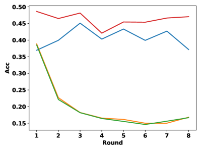
(a) 1-shot setting.

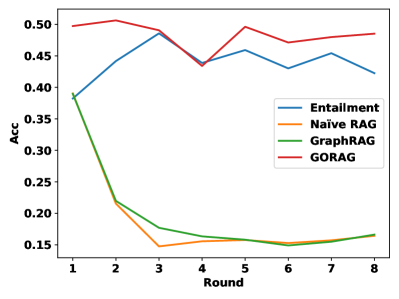
(b) 5-shot setting.

Figure 4. Experiment result of WOS dataset under 1-shot and 5-shot settings.

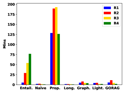
(a) Model Training/Indexing time on WOS dataset.

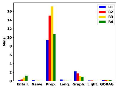
(b) Model Training/Indexing time on Reuters dataset.

Figure 5. Model Training/Indexing time on two datasets under 1-shot setting.

4.1.4. Hyperparameter and Hardware Settings

In each round of our experiments, we handle NN and RAG-based models differently for training and indexing. For NN-based models, we train them using all labeled data from the current round and all previous rounds. For RAG-based models, we index the labeled data of the current round to the information source from the previous round. The RAG-based model is initialized from scratch only in the first round.

After training or indexing in each round, we test the models using the testing data from the current round and all previous rounds. For GORAG, which employs an online indexing mechanism, we first test its performance with online indexing on the current round’s testing data. We then test its performance on the testing data from all previous rounds without online indexing. This approach allows us to study the effect of online indexing on the performance of later round data when applied to previous round data.

For the hyperparameter settings, we train the Entailment model with the RoBERTa-large PLM for 5 epochs with a batch size of 16, a learning rate of $1\times 10^{-6}$, and the Adam optimizer (Kingma, 2014), following the exact setting in Entailment’s original paper. For LongLLMLingua, we test the compression rate within ${0.75,0.8,0.85}$ and select 0.8, as it achieves the best overall classification accuracy. For GraphRAG and LightRAG, we use their local search mode, as it achieves the highest classification accuracy on both the WOS and Reuters datasets. For GORAG and all RAG-based baselines, we use LLaMA3 (Touvron et al., 2023) as the LLM backbone unless otherwise specified.

All experiments are conducted on an Intel(R) Xeon(R) Gold 5220R @ 2.20GHz CPU and a single NVIDIA A100-SXM4-40GB GPU.

4.2. Experiment Results

In this paper, we employ 1-shot, 5-shot, and 10-shot settings for few-shot training, where each setting corresponds to using 1, 5, and 10 labeled training samples per class, respectively. We omit experiments with more than 10 labeled samples per class, as for WOS dataset, there are already over 1300 labeled training data under 10-shot setting.

4.2.1. Effectiveness Evaluation

As shown in Table 3, GORAG achieves the best classification accuracy over all four rounds with 1-shot and 5-shot labeled indexing data on WOS dataset, it surpasses all RAG-based baselines as well as the state-of-the-art model Entailment. Compared with Entailment, when apply 1-shot setting, GORAG achieves at most 31.6% accuracy gain from 0.3695 to 0.4862 at the first round. On Reuters dataset, GORAG achieves the best classification accuracy over the last 3 rounds with 1-shot indexing data.

Furthermore, based on the experiment results in Table 3, we can have following observations. Firstly, for RAG-based models other than GORAG, although they can achieve comparable or even better performance than NN-based models in the first round, they tend to suffer a more significant performance drop as the number of labels increases. This is because the current RAG models compress the texts and ignore the compression of the target label set. As a result, when the number of target labels increases, the lengthy input can make the LLM tend to give wrong classification results and suffer from the lost-in-the-middle issue.

Secondly, compared with NN-based models, all RAG-based models other than GORAG are less sensitive to the increase of labeled data, from 1-shot to 5-shot setting on WOS dataset, the performance of Entailment increases significantly, however, for RAG-based baselines, performance tends to remain the same from 1-shot to 10-shot setting. This is because RAG-based models do not train any model parameters. Although an increase in training data can bring new information to enrich the side information, they are not always considered useful by the model and may not be retrieved. Consequently, the increase in labeled data may have no effect on some data samples during testing. On the other hand, for GORAG, the new information can introduce new paths for GORAG’s adaptive retrieval algorithm. This expands the influence scope of the new information from a fixed graph neighborhood to the entire information graph, making it easier for the retrieval process to benefit from the new information.

Thirdly, for Long Context RAG models, their lengthy retrieved side information further increase the length of LLM classification inputs, and consequently make the LLM harder to detect the relevence between side information and the labels than Compression based RAG models, exacerbating the lost-in-the-middle issue and make the LLM tend to generate wrong classification results.

4.2.2. Robustness Evaluation

To evaluate the robustness of GORAG and several representative baselines from the three technical categories, we conducted additional experiments on the 6 and 8 round split versions of the WOS dataset under 1-shot and 5-shot settings, as the WOS dataset contains more testing data than Reuters dataset. In Figure 4, the results for rounds 1 to 4 are obtained from the 4-round split version, rounds 5 and 6 are obtained from the 6-round split version, and rounds 7 and 8 are obtained from the 8-round split version of the WOS dataset. This setting ensures that the testing data at each round is as sufficient as possible while maintaining a acceptable amount of experiment time cost. As illustrated in Figure 4, the classification accuracy of GraphRAG and NaiveRAG drops significantly from round 1 to round 8, demonstrating the negative impact of the lengthy and unfiltered target label set on classification results. However, compared to other RAG-based baselines, GORAG maintains competitive classification accuracy as the number of rounds increases through 1 to 8 round, with both of the 1-shot and 5-shot setting.

Table 4. The size of the constructed information graph in each round.

Dataset	Model	Round
		R1		R2		R3		R4		After R4
		Node #	Edge #	Node #	Edge #	Node #	Edge #	Node #	Edge #	Node #	Edge #
WOS	GORAG offline	1,149	1,405	3,681	4,587	4,947	6,204	5,438	6,879	5,438	6,879
	GORAG	1,149	1,405	12,108	12,245	25,357	26,290	34,521	35,919	44,283	45,973
Reuters	GORAG offline	117	119	192	200	263	284	331	366	331	366
	GORAG	117	119	584	594	1,013	1,046	1,342	1,405	1,533	1,600

Table 5. 0-shot experiment result on WOS dataset.

Model	Round
	R1	R2	R3	R4
Qwen2.0-7B	0.3322	0.1790	0.1451	0.1444
Mistral0.3-7B	0.1436	0.0540	0.0336	0.0270
LLaMA3-8B	0.3351	0.1614	0.1161	0.0930
GORAG	0.3305	0.2567	0.2230	0.2102

4.2.3. Efficiency Evaluation

To evaluate the efficiency of GORAG, we compare GORAG’s indexing time cost with other baselines’ training or indexing time cost on the 4 round split version of WOS and Reuters datasets, the results are shown in Figure 5. For both datasets, Propositionizer achieves the worst indexing efficiency. This is because it employs an additional fine-tuned LLM to convert side information into propositions. In this process, this extra LLM generates a long list of propositions converted from each indexing or testing text, introducing more efficiency overhead compared to other models that use the LLM solely for classification, which typically generate only a few tokens representing the label name or label number.

On the WOS dataset, the indexing procedure of compression RAG-based models exhibits better time efficiency than the training procedure of NN-based models from R2 to R4. This is because NN-based models require retraining the entire model with all seen labeled data in each round, which limits their training efficiency.

On the Reuters dataset, GraphRAG achieves the worst indexing efficiency among all Compression RAG models. This is because the Reuters dataset contains fewer labels than the WOS dataset in each round. As a result, the constructed graph tends to be smaller than that of the WOS dataset, as shown in Table 4. Consequently, since the time cost of GraphRAG’s community generation procedure is also determined by the number of communities generated (Traag et al., 2019), GraphRAG introduces a more significant efficiency overhead on the Reuters dataset where the created information graph is much smaller compared to the WOS dataset.

4.3. Ablation Study

To further study GORAG’s zero-shot ability, we conducted an experiment on the WOS dataset by providing only the label names, without any labeled data to GORAG and some widely applied open-source LLM models, the result is shown in Table 5. In the 0-shot setting, GORAG first generates label descriptions based on the label names, then extracts keywords from these descriptions, without using any information from labeled texts. Note that the Entailment model cannot be applied in this setting, as they require labeled data for training or indexing. For RAG-based models, their performance in the 0-shot setting is equivalent to that of their backbone LLMs due to the lack of indexing data.

As shown by the results, GORAG achieves comparable performance with other open-source LLM models in the first round and outperforms them in all subsequent rounds. This is because, when the number of target labels is small, the benefit of compressing the target label set is not as pronounced. However, as the number of labels increases, the importance of filtering the label set becomes more significant, allowing GORAG to consistently outperform other open-source LLM models.

To better study the reason behind GORAG’s superior performance, we conduct an extensive ablation study under 1-shot setting on GORAG. For the ablation studie, we only experimented with the 1-shot setting unless further illustrated, as the performance of RAG models do not change significantly with different shot settings. Specifically, to better study how different components of GORAG affects the classification performance, we apply its following variants for ablation study:

• GORAG unit: The GORAG model that remove the edge weighting mechanim, every edge in this variant is assigned with weight 1.

• GORAG offline: The GORAG model that remove the online indexing mechanism.

• GORAG keyword: The GORAG model that only use the keyword extracted from the text to create LLM classification input, rather than the whole text.

Table 6. Ablation experiments for variants of GORAG.

Dataset	Model	Round
		R1	R2	R3	R4
WOS	GORAG unit	0.4706	0.4394	0.4407	0.3899
	GORAG offline	0.3063	0.2302	0.2455	0.2156
	GORAG keyword	0.4746	0.4606	0.4455	0.4030
	GORAG	0.4862	0.4649	0.4814	0.4210
Reuters	GORAG unit	0.0000	0.0625	0.1667	0.0795
	GORAG offline	0.0000	0.1000	0.0917	0.1032
	GORAG keyword	0.0000	0.1000	0.1167	0.1438
	GORAG	0.0875	0.1750	0.1667	0.1667

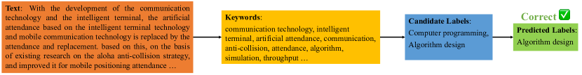
(a) GORAG’s candidate selection algorithm returns candidate labels adaptively based on keywords extracted from the tesing texts.

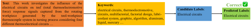
(b) GORAG’s candidate selection algorithm only returns the ground truth label of the testing text.

Figure 6. Two case of GORAG successfully generate candidate labels to help text classification on WOS dataset.

In Table 6, we present the results of these variants to evaluate whether the edge weighting mechanism, the online indexing mechanism, and the substitution of lengthy texts with shorter keywords can enhance the prediction accuracy of GORAG. The results show that GORAG achieves the best prediction accuracy, demonstrating the importance of the edge weighting and onling indexing mechanism. Furthermore, GORAG keyword also achieves a competitive performance, illustrating the keywords extracted from texts can also have valuable information for text classification.

Table 7. Evaluation on different LLM backbones.

Dataset	Model	Round
		R1	R2	R3	R4
WOS	GORAG LLaMA3	0.4862	0.4649	0.4814	0.4210
	GORAG Qwen2.5	0.5101	0.4839	0.4823	0.4235

Additionally, in Table 4, we compare the size of the constructed information graph with and without online indexing after each round. After applying the online indexing mechanism, the information graph being significantly enriched from R1 to After R4.

In Table 7, we present the results of GORAG with different backbone LLMs, we test GORAG with more advanced Qwen2.5-7B (Qwen Team, 2024), the result demonstates the GORAG’s performance can be further improved with more advanced LLM backbones.

4.4. Case Study

In this subsection, to illustrate the strength of GORAG’s adaptive retrieval and candidate label generation procedure, we dig into two testing cases select from WOS dataset where GORAG’s adaptive retrieval helps to reduce the LLM input length and benefit text classification. As shown in Figure 6(a), for the case whose ground truth label is Algorithm Design, the candidate label retrieved by GORAG are Computer programming and Algorithm design. As a result, GORAG’s adaptive retrieval algorithm successfully filter the target label set to only contains two candidate labels, and successfully cut down the target label number from at most over 100 to only 2 candidate labels that it consided as the possible labels for the text, significantlly reduce the LLM’s input length and mitigate the lost-in-the-middle issue.

On the other hand, for the case in Figure 6(b) whose ground truth label is Electrical Circuits, since the ground truth label name Electrical Circuits already exists in the text and being extracted as keyword, GORAG’s adaptive retrieval algorithm is almost certain to classify this text into class Electrical Circuits, hence GORAG’s adaptive retrieval and candidate type generation algorithm would only select the only candidate label retrieved from the constructed graph and input to the LLM.

4.5. Discussion

According to the aforementioned experimental results, we have identified several key characteristics of NN-based models and RAG-based models.

On the one hand, despite the rapid development of LLMs in recent years, they can still yield sub-optimal classification accuracy in DFSTC tasks due to the lengthy LLM inputs. When there is a sufficient amount of labeled data available in each dynamic updation round, the NN-based model Entailment can also achieve comparable or even better performance than traditional RAG based models other than GORAG.

On the other hand, compared with NN-based models, benefited from the time efficient indexing of the side information and the rich pre-trained knowledge within the LLM, by filter out some unrelated labels and shorten the LLM inputs, RAG-based models are better suited for DFSTC task when the target labels are updated frequently and there only existes a limit number or even none of the labeled data is avaiable for each dynamic updation round.

5. Conclusion

In this paper, we propose GORAG, a Graph-based Online Retrieval Augmented Generation framework for the Dynamic Few-shot Text Classification (DFSTC) task. Extensive experiments on two text datasets with different characteristics demonstrate the effectiveness of GORAG in classifying texts with only a limited number or even no labeled data. Additionally, GORAG shows its effectiveness in adapting to the dynamic updates of target labels by retrieving candidate labels to filter the large target label set in each update round. With extensive of ablation studies, we confirm that GORAG’s adaptive retrieval, edge weighting, and online indexing mechanisms contribute to its effectiveness. For future work, we aim to further enhance GORAG’s performance and explore its application in more complex and diverse scenarios, as well as further improve the efficiency of GORAG’s online indexing mechanism.

References

- (1)
- imd ([n.d.]) [n.d.]. https://developer.imdb.com/non-commercial-datasets/. [Accessed 08-11-2024].
- nan ([n.d.]) [n.d.]. GitHub - gusye1234/nano-graphrag: A simple, easy-to-hack GraphRAG implementation — github.com. https://github.com/gusye1234/nano-graphrag. [Accessed 23-11-2024].
- Achiam et al. (2023) Josh Achiam, Steven Adler, Sandhini Agarwal, Lama Ahmad, Ilge Akkaya, Florencia Leoni Aleman, Diogo Almeida, Janko Altenschmidt, Sam Altman, Shyamal Anadkat, et al. 2023. Gpt-4 technical report. arXiv preprint arXiv:2303.08774 (2023).
- Aljehani et al. (2024) Amani Aljehani, Syed Hamid Hasan, and Usman Ali Khan. 2024. Advancing Text Classification: A Systematic Review of Few-Shot Learning Approaches. International Journal of Computing and Digital Systems 16, 1 (2024), 1–14.
- Amer-Yahia et al. (2023) Sihem Amer-Yahia, Angela Bonifati, Lei Chen, Guoliang Li, Kyuseok Shim, Jianliang Xu, and Xiaochun Yang. 2023. From Large Language Models to Databases and Back: A Discussion on Research and Education. SIGMOD Rec. 52, 3 (2023), 49–56. https://doi.org/10.1145/3631504.3631518
- Arora et al. (2023) Simran Arora, Brandon Yang, Sabri Eyuboglu, Avanika Narayan, Andrew Hojel, Immanuel Trummer, and Christopher Ré. 2023. Language Models Enable Simple Systems for Generating Structured Views of Heterogeneous Data Lakes. Proceedings of the VLDB Endowment 17, 2 (2023), 92–105.
- Bansal et al. (2020) Trapit Bansal, Rishikesh Jha, and Andrew Mccallum. 2020. Learning to Few-Shot Learn Across Diverse Natural Language Classification Tasks. In Proceedings of the 28th International Conference on Computational Linguistics. 5108–5123.
- Bao et al. (2020) Yujia Bao, Menghua Wu, Shiyu Chang, and Regina Barzilay. 2020. Few-shot Text Classification with Distributional Signatures. In International Conference on Learning Representations.
- Chen et al. (2023) Tong Chen, Hongwei Wang, Sihao Chen, Wenhao Yu, Kaixin Ma, Xinran Zhao, Hongming Zhang, and Dong Yu. 2023. Dense x retrieval: What retrieval granularity should we use? arXiv preprint arXiv:2312.06648 (2023).
- Devlin (2018) Jacob Devlin. 2018. Bert: Pre-training of deep bidirectional transformers for language understanding. arXiv preprint arXiv:1810.04805 (2018).
- Dieng et al. (2017) Adji B Dieng, Jianfeng Gao, Chong Wang, and John Paisley. 2017. TopicRNN: A recurrent neural network with long-range semantic dependency. In 5th International Conference on Learning Representations, ICLR 2017.
- Dong and Rekatsinas (2018) Xin Luna Dong and Theodoros Rekatsinas. 2018. Data integration and machine learning: A natural synergy. In Proceedings of the 2018 international conference on management of data. 1645–1650.
- Dong et al. (2023) Yuyang Dong, Chuan Xiao, Takuma Nozawa, Masafumi Enomoto, and Masafumi Oyamada. 2023. DeepJoin: Joinable Table Discovery with Pre-Trained Language Models. Proceedings of the VLDB Endowment 16, 10 (2023), 2458–2470.
- Du et al. (2024) Xingyu Du, Gongsheng Yuan, Sai Wu, Gang Chen, and Peng Lu. 2024. In Situ Neural Relational Schema Matcher. In 2024 IEEE 40th International Conference on Data Engineering (ICDE). IEEE, 138–150.
- Edge et al. (2024) Darren Edge, Ha Trinh, Newman Cheng, Joshua Bradley, Alex Chao, Apurva Mody, Steven Truitt, and Jonathan Larson. 2024. From local to global: A graph rag approach to query-focused summarization. arXiv preprint arXiv:2404.16130 (2024).
- Fan et al. (2024) Meihao Fan, Xiaoyue Han, Ju Fan, Chengliang Chai, Nan Tang, Guoliang Li, and Xiaoyong Du. 2024. Cost-effective in-context learning for entity resolution: A design space exploration. In 2024 IEEE 40th International Conference on Data Engineering (ICDE). IEEE, 3696–3709.
- Fernandez et al. (2023) Raul Castro Fernandez, Aaron J. Elmore, Michael J. Franklin, Sanjay Krishnan, and Chenhao Tan. 2023. How Large Language Models Will Disrupt Data Management. , 3302–3309 pages. https://doi.org/10.14778/3611479.3611527
- Gao et al. (2023) Yunfan Gao, Yun Xiong, Xinyu Gao, Kangxiang Jia, Jinliu Pan, Yuxi Bi, Yi Dai, Jiawei Sun, Meng Wang, and Haofen Wang. 2023. Retrieval-augmented generation for large language models: A survey. arXiv preprint arXiv:2312.10997 (2023).
- Gu et al. (2023) Zihui Gu, Ju Fan, Nan Tang, Lei Cao, Bowen Jia, Sam Madden, and Xiaoyong Du. 2023. Few-shot text-to-sql translation using structure and content prompt learning. Proceedings of the ACM on Management of Data 1, 2 (2023), 1–28.
- Guo et al. (2024) Zirui Guo, Lianghao Xia, Yanhua Yu, Tu Ao, and Chao Huang. 2024. LightRAG: Simple and Fast Retrieval-Augmented Generation. (2024). arXiv:2410.05779 [cs.IR]
- Gutiérrez et al. (2024) Bernal Jiménez Gutiérrez, Yiheng Shu, Yu Gu, Michihiro Yasunaga, and Yu Su. 2024. HippoRAG: Neurobiologically Inspired Long-Term Memory for Large Language Models. arXiv preprint arXiv:2405.14831 (2024).
- Hanmo et al. (2024) LIU Hanmo, DI Shimin, LI Haoyang, LI Shuangyin, CHEN Lei, and ZHOU Xiaofang. 2024. Effective Data Selection and Replay for Unsupervised Continual Learning. In 2024 IEEE 40th International Conference on Data Engineering (ICDE). IEEE, 1449–1463.
- Jiang et al. (2023) Albert Q Jiang, Alexandre Sablayrolles, Arthur Mensch, Chris Bamford, Devendra Singh Chaplot, Diego de las Casas, Florian Bressand, Gianna Lengyel, Guillaume Lample, Lucile Saulnier, et al. 2023. Mistral 7B. arXiv preprint arXiv:2310.06825 (2023).
- Jiang et al. (2024) Huiqiang Jiang, Qianhui Wu, , Xufang Luo, Dongsheng Li, Chin-Yew Lin, Yuqing Yang, and Lili Qiu. 2024. LongLLMLingua: Accelerating and Enhancing LLMs in Long Context Scenarios via Prompt Compression. In Proceedings of the 62nd Annual Meeting of the Association for Computational Linguistics (Volume 1: Long Papers), Lun-Wei Ku, Andre Martins, and Vivek Srikumar (Eds.). Association for Computational Linguistics, Bangkok, Thailand, 1658–1677. https://aclanthology.org/2024.acl-long.91
- Johnson and Zhang (2015) Rie Johnson and Tong Zhang. 2015. Semi-supervised convolutional neural networks for text categorization via region embedding. Advances in neural information processing systems 28 (2015).
- Johnson and Zhang (2017) Rie Johnson and Tong Zhang. 2017. Deep pyramid convolutional neural networks for text categorization. In Proceedings of the 55th Annual Meeting of the Association for Computational Linguistics (Volume 1: Long Papers). 562–570.
- Kayali et al. (2024) Moe Kayali, Anton Lykov, Ilias Fountalis, Nikolaos Vasiloglou, Dan Olteanu, and Dan Suciu. 2024. Chorus: Foundation Models for Unified Data Discovery and Exploration. Proceedings of the VLDB Endowment 17, 8 (2024), 2104–2114.
- Kim (2014) Yoon Kim. 2014. Convolutional Neural Networks for Sentence Classification. In Proceedings of the 2014 Conference on Empirical Methods in Natural Language Processing, EMNLP 2014, October 25-29, 2014, Doha, Qatar, A meeting of SIGDAT, a Special Interest Group of the ACL, Alessandro Moschitti, Bo Pang, and Walter Daelemans (Eds.). ACL, 1746–1751. https://doi.org/10.3115/V1/D14-1181
- Kingma (2014) Diederik P Kingma. 2014. Adam: A method for stochastic optimization. arXiv preprint arXiv:1412.6980 (2014).
- Kouadri et al. (2020) Wissam Mammar Kouadri, Mourad Ouziri, Salima Benbernou, Karima Echihabi, Themis Palpanas, and Iheb Ben Amor. 2020. Quality of sentiment analysis tools: The reasons of inconsistency. Proceedings of the VLDB Endowment 14, 4 (2020), 668–681.
- Kowsari et al. (2017) Kamran Kowsari, Donald E Brown, Mojtaba Heidarysafa, Kiana Jafari Meimandi, Matthew S Gerber, and Laura E Barnes. 2017. Hdltex: Hierarchical deep learning for text classification. In 2017 16th IEEE international conference on machine learning and applications (ICMLA). IEEE, 364–371.
- Kowsari et al. (2019) Kamran Kowsari, Kiana Jafari Meimandi, Mojtaba Heidarysafa, Sanjana Mendu, Laura Barnes, and Donald Brown. 2019. Text classification algorithms: A survey. Information 10, 4 (2019), 150.
- Li et al. (2024) Boyan Li, Yuyu Luo, Chengliang Chai, Guoliang Li, and Nan Tang. 2024. The Dawn of Natural Language to SQL: Are We Fully Ready? [Experiment, Analysis \u0026 Benchmark ]. Proc. VLDB Endow. 17, 11 (2024), 3318–3331. https://www.vldb.org/pvldb/vol17/p3318-luo.pdf
- Li et al. (2022) Qian Li, Hao Peng, Jianxin Li, Congying Xia, Renyu Yang, Lichao Sun, Philip S Yu, and Lifang He. 2022. A survey on text classification: From traditional to deep learning. ACM Transactions on Intelligent Systems and Technology (TIST) 13, 2 (2022), 1–41.
- Liu et al. (2024) Nelson F Liu, Kevin Lin, John Hewitt, Ashwin Paranjape, Michele Bevilacqua, Fabio Petroni, and Percy Liang. 2024. Lost in the middle: How language models use long contexts. Transactions of the Association for Computational Linguistics 12 (2024), 157–173.
- Liu et al. (2016) Pengfei Liu, Xipeng Qiu, and Xuanjing Huang. 2016. Recurrent neural network for text classification with multi-task learning. In Proceedings of the Twenty-Fifth International Joint Conference on Artificial Intelligence. 2873–2879.
- Liu et al. (2023) Pengfei Liu, Weizhe Yuan, Jinlan Fu, Zhengbao Jiang, Hiroaki Hayashi, and Graham Neubig. 2023. Pre-train, prompt, and predict: A systematic survey of prompting methods in natural language processing. Comput. Surveys 55, 9 (2023), 1–35.
- Liu (2019) Yinhan Liu. 2019. Roberta: A robustly optimized bert pretraining approach. arXiv preprint arXiv:1907.11692 (2019).
- Mehlhorn (1988) Kurt Mehlhorn. 1988. A faster approximation algorithm for the Steiner problem in graphs. Inform. Process. Lett. 27, 3 (1988), 125–128. https://doi.org/10.1016/0020-0190(88)90066-X
- Meng et al. (2018) Yu Meng, Jiaming Shen, Chao Zhang, and Jiawei Han. 2018. Weakly-supervised neural text classification. In proceedings of the 27th ACM International Conference on information and knowledge management. 983–992.
- Meng et al. (2020) Yu Meng, Yunyi Zhang, Jiaxin Huang, Chenyan Xiong, Heng Ji, Chao Zhang, and Jiawei Han. 2020. Text classification using label names only: A language model self-training approach. arXiv preprint arXiv:2010.07245 (2020).
- Miao et al. (2024) Xupeng Miao, Zhihao Jia, and Bin Cui. 2024. Demystifying Data Management for Large Language Models. In Companion of the 2024 International Conference on Management of Data, SIGMOD/PODS 2024, Santiago AA, Chile, June 9-15, 2024, Pablo Barceló, Nayat Sánchez-Pi, Alexandra Meliou, and S. Sudarshan (Eds.). ACM, 547–555. https://doi.org/10.1145/3626246.3654683
- Miao et al. (2021) Zhengjie Miao, Yuliang Li, and Xiaolan Wang. 2021. Rotom: A meta-learned data augmentation framework for entity matching, data cleaning, text classification, and beyond. In Proceedings of the 2021 International Conference on Management of Data. 1303–1316.
- Minaee et al. (2021) Shervin Minaee, Nal Kalchbrenner, Erik Cambria, Narjes Nikzad, Meysam Chenaghlu, and Jianfeng Gao. 2021. Deep learning–based text classification: a comprehensive review. ACM computing surveys (CSUR) 54, 3 (2021), 1–40.
- Pan et al. (2024) Zhuoshi Pan, Qianhui Wu, Huiqiang Jiang, Menglin Xia, Xufang Luo, Jue Zhang, Qingwei Lin, Victor Ruhle, Yuqing Yang, Chin-Yew Lin, H. Vicky Zhao, Lili Qiu, and Dongmei Zhang. 2024. LLMLingua-2: Data Distillation for Efficient and Faithful Task-Agnostic Prompt Compression. In Proceedings of the 62nd Annual Meeting of the Association for Computational Linguistics (Volume 1: Long Papers), Lun-Wei Ku, Andre Martins, and Vivek Srikumar (Eds.). Association for Computational Linguistics, Bangkok, Thailand, 963–981. https://aclanthology.org/2024.findings-acl.57
- Parisi et al. (2019) German I Parisi, Ronald Kemker, Jose L Part, Christopher Kanan, and Stefan Wermter. 2019. Continual lifelong learning with neural networks: A review. Neural networks 113 (2019), 54–71.
- Peters et al. (2018) Matthew E. Peters, Mark Neumann, Mohit Iyyer, Matt Gardner, Christopher Clark, Kenton Lee, and Luke Zettlemoyer. 2018. Deep Contextualized Word Representations. In Proceedings of the 2018 Conference of the North American Chapter of the Association for Computational Linguistics: Human Language Technologies, Volume 1 (Long Papers), Marilyn Walker, Heng Ji, and Amanda Stent (Eds.). Association for Computational Linguistics, New Orleans, Louisiana, 2227–2237. https://doi.org/10.18653/v1/N18-1202
- Prieto et al. (2016) Alberto Prieto, Beatriz Prieto, Eva Martinez Ortigosa, Eduardo Ros, Francisco Pelayo, Julio Ortega, and Ignacio Rojas. 2016. Neural networks: An overview of early research, current frameworks and new challenges. Neurocomputing 214 (2016), 242–268.
- Qwen Team (2024) Qwen Team. 2024. Qwen2.5: A Party of Foundation Models. https://qwenlm.github.io/blog/qwen2.5/
- Ren et al. (2024) Tonghui Ren, Yuankai Fan, Zhenying He, Ren Huang, Jiaqi Dai, Can Huang, Yinan Jing, Kai Zhang, Yifan Yang, and X. Sean Wang. 2024. PURPLE: Making a Large Language Model a Better SQL Writer. In 40th IEEE International Conference on Data Engineering, ICDE 2024, Utrecht, The Netherlands, May 13-16, 2024. IEEE, 15–28. https://doi.org/10.1109/ICDE60146.2024.00009
- Sahay et al. (2020) Tanvi Sahay, Ankita Mehta, and Shruti Jadon. 2020. Schema matching using machine learning. In 2020 7th International Conference on Signal Processing and Integrated Networks (SPIN). IEEE, 359–366.
- Sammut and Webb (2010) Claude Sammut and Geoffrey I. Webb (Eds.). 2010. TF–IDF. Springer US, Boston, MA, 986–987. https://doi.org/10.1007/978-0-387-30164-8_832
- Sarthi et al. (2024) Parth Sarthi, Salman Abdullah, Aditi Tuli, Shubh Khanna, Anna Goldie, and Christopher D Manning. 2024. Raptor: Recursive abstractive processing for tree-organized retrieval. arXiv preprint arXiv:2401.18059 (2024).
- Su et al. (2020) Ke Su, Bing Lu, Huang Ngo, Panos M. Pardalos, and Ding-Zhu Du. 2020. Steiner Tree Problems. Springer International Publishing, Cham, 1–15. https://doi.org/10.1007/978-3-030-54621-2_645-1
- Sun et al. (2021) Yu Sun, Shuohuan Wang, Shikun Feng, Siyu Ding, Chao Pang, Junyuan Shang, Jiaxiang Liu, Xuyi Chen, Yanbin Zhao, Yuxiang Lu, et al. 2021. Ernie 3.0: Large-scale knowledge enhanced pre-training for language understanding and generation. arXiv preprint arXiv:2107.02137 (2021).
- Touvron et al. (2023) Hugo Touvron, Thibaut Lavril, Gautier Izacard, Xavier Martinet, Marie-Anne Lachaux, Timothée Lacroix, Baptiste Rozière, Naman Goyal, Eric Hambro, Faisal Azhar, et al. 2023. Llama: Open and efficient foundation language models. arXiv preprint arXiv:2302.13971 (2023).
- Traag et al. (2019) Vincent A Traag, Ludo Waltman, and Nees Jan Van Eck. 2019. From Louvain to Leiden: guaranteeing well-connected communities. Scientific reports 9, 1 (2019), 1–12.
- Trummer (2022) Immanuel Trummer. 2022. From BERT to GPT-3 codex: harnessing the potential of very large language models for data management. Proceedings of the VLDB Endowment 15, 12 (2022), 3770–3773.
- Tu et al. (2023) Jianhong Tu, Ju Fan, Nan Tang, Peng Wang, Guoliang Li, Xiaoyong Du, Xiaofeng Jia, and Song Gao. 2023. Unicorn: A unified multi-tasking model for supporting matching tasks in data integration. Proceedings of the ACM on Management of Data 1, 1 (2023), 1–26.
- Wang et al. (2024) Liyuan Wang, Xingxing Zhang, Hang Su, and Jun Zhu. 2024. A comprehensive survey of continual learning: theory, method and application. IEEE Transactions on Pattern Analysis and Machine Intelligence (2024).
- Wang et al. (2018) Yequan Wang, Aixin Sun, Jialong Han, Ying Liu, and Xiaoyan Zhu. 2018. Sentiment analysis by capsules. In Proceedings of the 2018 world wide web conference. 1165–1174.
- Wang et al. (2020) Yaqing Wang, Quanming Yao, James T Kwok, and Lionel M Ni. 2020. Generalizing from a few examples: A survey on few-shot learning. ACM computing surveys (csur) 53, 3 (2020), 1–34.
- Wang et al. (2017) Zhiguo Wang, Wael Hamza, and Radu Florian. 2017. Bilateral multi-perspective matching for natural language sentences. In Proceedings of the 26th International Joint Conference on Artificial Intelligence. 4144–4150.
- Xia et al. (2021) Congying Xia, Wenpeng Yin, Yihao Feng, and Philip S. Yu. 2021. Incremental Few-shot Text Classification with Multi-round New Classes: Formulation, Dataset and System. In Proceedings of the 2021 Conference of the North American Chapter of the Association for Computational Linguistics: Human Language Technologies, NAACL-HLT 2021, Online, June 6-11, 2021, Kristina Toutanova, Anna Rumshisky, Luke Zettlemoyer, Dilek Hakkani-Tür, Iz Beltagy, Steven Bethard, Ryan Cotterell, Tanmoy Chakraborty, and Yichao Zhou (Eds.). Association for Computational Linguistics, 1351–1360. https://doi.org/10.18653/V1/2021.NAACL-MAIN.106
- Yang et al. (2024) An Yang, Baosong Yang, Binyuan Hui, Bo Zheng, Bowen Yu, Chang Zhou, Chengpeng Li, Chengyuan Li, Dayiheng Liu, Fei Huang, et al. 2024. Qwen2 technical report. arXiv preprint arXiv:2407.10671 (2024).
- Yang et al. (2019) Zhilin Yang, Zihang Dai, Yiming Yang, Jaime Carbonell, Ruslan Salakhutdinov, and Quoc V. Le. 2019. XLNet: generalized autoregressive pretraining for language understanding. Curran Associates Inc., Red Hook, NY, USA.
- Yu and Litchfield (2020) Hang Yu and Lester Litchfield. 2020. Query classification with multi-objective backoff optimization. In Proceedings of the 43rd International ACM SIGIR Conference on Research and Development in Information Retrieval. 1925–1928.
- Yu et al. (2023) Tianhuan Yu, Zhenying He, Zhihui Yang, Fei Ye, Yuankai Fan, Yinan Jing, Kai Zhang, and X Sean Wang. 2023. Zebra: A novel method for optimizing text classification query in overload scenario. World Wide Web 26, 3 (2023), 905–931.
- Zhang et al. (2024b) Meihui Zhang, Zhaoxuan Ji, Zhaojing Luo, Yuncheng Wu, and Chengliang Chai. 2024b. Applications and Challenges for Large Language Models: From Data Management Perspective. In 40th IEEE International Conference on Data Engineering, ICDE 2024, Utrecht, The Netherlands, May 13-16, 2024. IEEE, 5530–5541. https://doi.org/10.1109/ICDE60146.2024.00441
- Zhang et al. (2023a) Ranran Haoran Zhang, Aysa Xuemo Fan, and Rui Zhang. 2023a. ConEntail: An Entailment-based Framework for Universal Zero and Few Shot Classification with Supervised Contrastive Pretraining. In Proceedings of the 17th Conference of the European Chapter of the Association for Computational Linguistics. 1941–1953.
- Zhang et al. (2024a) Yu Zhang, Mei Di, Haozheng Luo, Chenwei Xu, and Richard Tzong-Han Tsai. 2024a. SMUTF: Schema Matching Using Generative Tags and Hybrid Features. arXiv preprint arXiv:2402.01685 (2024).
- Zhang et al. (2023b) Yunjia Zhang, Avrilia Floratou, Joyce Cahoon, Subru Krishnan, Andreas C Müller, Dalitso Banda, Fotis Psallidas, and Jignesh M Patel. 2023b. Schema matching using pre-trained language models. In 2023 IEEE 39th International Conference on Data Engineering (ICDE). IEEE, 1558–1571.
- Zhang et al. (2023c) Yue Zhang, Yafu Li, Leyang Cui, Deng Cai, Lemao Liu, Tingchen Fu, Xinting Huang, Enbo Zhao, Yu Zhang, Yulong Chen, et al. 2023c. Siren’s song in the AI ocean: a survey on hallucination in large language models. arXiv preprint arXiv:2309.01219 (2023).