Resonance fluorescence spectra of a driven Kerr nonlinear resonator

Abstract

Resonance fluorescence spectra of a driven Kerr nonlinear resonator is investigated both theoretically and experimentally. When the Kerr nonlinear resonator is driven strongly such that the induced Rabi frequency is comparable to or larger than the Kerr nonlinearity, the system cannot be approximated as a two-level system. We theoretically derive characteristic features in the fluorescence spectra such as the decrease of the center-peak intensity and the asymmetric sideband peaks in the presence of finite dephasing. Those features are consistently explained by the population of the initial dressed state and its transition matrix element to the final dressed state of the transition corresponding to each peak. Finally, we experimentally measure the resonance fluorescence spectra of a driven superconducting Kerr nonlinear resonator and find a quantitative agreement with our theory.

I Introduction

Resonance fluorescence is a fundamental phenomenon of quantum optics manifesting coherent light–matter interactions Mollow (1969); Kimble and Mandel (1976). It was first observed in atomic systems Schuda et al. (1974); Wu et al. (1975), and more recently in artificial-atom systems such as semiconductor quantum dots Muller et al. (2007) and superconducting circuits Astafiev et al. (2010).

In superconducting systems, referred to as a circuit-quantum-electrodynamics system Blais et al. (2004); Gu et al. (2017), resonance fluorescence has been extensively studied in the contexts of photon blockade Lang et al. (2011), creation of super- and subradiant states van Loo et al. (2013), qubit readout using squeezed microwaves Toyli et al. (2016), and characterization of qubit decoherence rates Lu et al. (2021). Most of these studies successfully treated the qubit as a two-level system with an exception of Ref. Gasparinetti et al. (2017), where they observed two-photon resonance fluorescence involving a second excited state of a transmon qubit. However, superconducting qubits are essentially a multi-level system, and it is expected that such a two-level approximation becomes invalid if the qubit is driven so strongly that the induced Rabi frequency is comparable to the anharmonicity of the qubit. It is also worth mentioning that the resonance fluorescence in three-level systems with $\Lambda$-, $V$- and $\Xi$-type energy-level configurations has been studied both in theory Fu et al. (1992) and experiment in the atomic system Tian et al. (2012).

Energy levels of the dressed states in the strong-drive regime, where the Rabi frequency is comparable to the anharmonicity, has been probed spectroscopically in a transmon qubit Baur et al. (2009); Koshino et al. (2013) and a Kerr parametric oscillator (KPO) Yamaji et al. (2022). However, fluorescence under the strong-drive regime has not been reported.

In the present work, we theoretically and experimentally study the fluorescence from a nonlinear resonator with Kerr nonlinearity. In the theory, we develop a general formalism for the fluorescence spectrum, and apply it to a transmon qubit Koch et al. (2007) and a Kerr nonlinear resonator (KNR) Goto (2016a); Puri et al. (2017a), which have different magnitudes of the Kerr nonlinearity, to compare them with an ideal two-level system. In the experiment, we use a KNR with the nonlinearity of around 10 MHz, which is one order smaller than that of a typical transmon qubit and is therefore suitable for realizing the strong-drive regime.

The present paper is organized as follows. In Sec. II, we develop a general formalism of the coherent and incoherent scatterings of an external drive field by a KNR, latter of which gives fluorescence spectrum of the KNR. Using the theory, we calculate the resonance-fluorescence spectrum of a strongly driven KNR. We observe that the spectrum exhibits characteristic features, which are distinct from the cases of a two-level system and a weakly driven KNR. We also show that those features can be explained in terms of the state population and the transition matrix element for the corresponding transition. Section III describes our experiments. We measure the resonance fluorescence of a superconducting KNR and confirm that the observed spectrum is well reproduced by our theory. Finally, we conclude our discussion in Sec. IV.

II Theory

II.1 Calculation of the fluorescence spectra

Figure 1 shows a schematic diagram of the system we consider in this study. A Kerr nonlinear resonator (KNR) is coupled to the signal port, which is a semi-infinite transmission line to apply a drive field to the KNR. The KNR is also coupled to fictitious loss ports to account for its internal loss and dephasing. Here we assume dephasing due to the Markovian noise. The Hamiltonian of the system is given by

$$\mathcal{H} = \mathcal{H}_{\rm sys}+\mathcal{H}_{\rm sig}+\mathcal{H}_{\rm loss}+\mathcal{H}_{\rm dep},$$ (1)

$$\mathcal{H}_{\rm sys}/\hbar = \Omega_{0}a^{\dagger}a+\frac{K}{2}a^{\dagger}a^{\dagger}aa,$$ (2)

$$\mathcal{H}_{\rm sig}/\hbar = \int dk\Bigl{[}v_{b}kb_{k}^{\dagger}b_{k}+\sqrt{\frac{v_{b}\kappa_{\rm ex}}{2\pi}}\,\Bigl{(}a^{\dagger}b_{k}+b_{k}^{\dagger}a\Bigr{)}\Bigr{]},$$ (3)

$$\mathcal{H}_{\rm loss}/\hbar = \int dk\Bigl{[}v_{c}kc_{k}^{\dagger}c_{k}+\sqrt{\frac{v_{c}\kappa_{\rm in}}{2\pi}}\,\Bigl{(}a^{\dagger}c_{k}+c_{k}^{\dagger}a\Bigr{)}\Bigr{]},$$ (4)

$$\mathcal{H}_{\rm dep}/\hbar = \int dk\Bigl{[}v_{d}kd_{k}^{\dagger}d_{k}+\sqrt{\frac{v_{d}\gamma_{\rm p}}{\pi}}\,a^{\dagger}a\Bigl{(}d_{k}+d_{k}^{\dagger}\Bigr{)}\Bigr{]}.$$ (5)

Here, $\Omega_{0}$ and $K$ represent the resonance frequency and the Kerr nonlinearity of the resonator, respectively, and $a$ is an annihilation operator for the resonator mode, which satisfies $[a,a^{\dagger}]=1$. The field operator in the wave-number representation, $b_{k}$, is for the mode in the signal port with the wave number $k$ and velocity $v_{b}$. The coupling between the resonator and the signal port is denoted by $\kappa_{\rm ex}$, the external coupling rate. Similarly, $c_{k}$ and $d_{k}$ are field operators for the fictitious loss ports describing the internal loss and dephasing, respectively. Their coupling strengths, $\kappa_{\rm in}$ and $\gamma_{\rm p}$, correspond to the internal loss and dephasing rates, respectively. The operators $b_{k}$, $c_{k}$ and $d_{k}$ satisfy the following commutation rules: $\bigl{[}b_{k},b^{\dagger}_{k^{\prime}}\bigr{]}=\bigl{[}c_{k},c^{\dagger}_{k^{\prime}}\bigr{]}=\bigl{[}d_{k},d^{\dagger}_{k^{\prime}}\bigr{]}=\delta(k-k^{\prime})$. Hereafter, we assume that $v_{b}=v_{c}=v_{d}$ for simplicity and denote them by $v$.

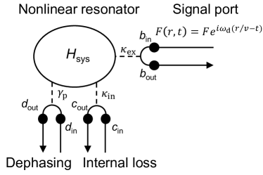
Figure 1:   System under consideration.

Because of the continuous driving, the KNR is expected to show fluorescence, which is contained in the $b_{\rm out}$ field as an incoherent component. In fact, an analytical formula of the fluorescence spectra for a two-level sysmtem has been derived in Refs. Koshino and Nakamura (2012); Lu et al. (2021). Here, we extend it for a multi-level system, namely, the Kerr nonlinear resonator. Below we show the outline of the calculation. The details are explained in Appendix A. Note that, in contrast to the case of a two-level system, we cannot obtain a compact analytic expression for the fluorescence spectra for a KNR. They are calculated after solving a set of simultaneous equations involving an infinite number of variables by truncation.

We assume that, at $t$=0, the overall system is in its ground state and a drive field $\mathcal{F}(r/v-t)$ is injected from the signal port, where

$$\mathcal{F}(r/v-t)=Fe^{\mathrm{i}\omega_{\rm d}(r/v-t)}/\sqrt{v}.$$ (6)

Here, $\omega_{\rm d}$ is the angular frequency of the drive field and $F$ is its amplitude in units of $1/\sqrt{\mathrm{s}}$. Note that $|F|^{2}$ represents the photon rate. In the steady state, the power spectrum of the output field $b_{\rm out}(t)$ is given by

$$S(\omega)=\operatorname{Re}\int_{0}^{\infty}\frac{d\tau}{\pi}e^{\mathrm{i}\omega\tau}\langle b_{\rm out}^{\dagger}(t)b_{\rm out}(t+\tau)\rangle,$$ (7)

where the bracket represents the expectation value calulated with the initial state vector [Eq. (38)], which is the eigenstate of the input field $b_{\rm in}(t)$. Using the input–output relation

$$~b_{\rm out}(t)=b_{\rm in}(t)-\mathrm{i}\sqrt{\frac{\kappa_{\rm ex}}{v}}\,a(t),$$ (8)

we obtain the following formula

$$S(\omega) \equiv S_{\rm c}(\omega)+S_{\rm i}(\omega)$$ (9)

$$S_{\rm c}(\omega) = \operatorname{Re}\int_{0}^{\infty}\frac{d\tau}{\pi}e^{\mathrm{i}\omega\tau}\langle b_{\rm out}^{\dagger}(t)\rangle\langle b_{\rm out}(t+\tau)\rangle$$ (10)

$$S_{\rm i}(\omega) = \operatorname{Re}\int_{0}^{\infty}\frac{d\tau}{\pi}e^{\mathrm{i}\omega\tau}\frac{\kappa_{\rm ex}}{v}\langle a^{\dagger}(t),a(t+\tau)\rangle,$$ (11)

where $S_{\rm c}(\omega)$ and $S_{\rm i}(\omega)$ represent coherent and incoherent components, respectively, and $\langle A,B\rangle\equiv\langle AB\rangle-\langle A\rangle\langle B\rangle$.

II.1.1 Calculation of the two-time correlation function

In order to evaluate $\langle a^{\dagger}(t),a(t+\tau)\rangle$ in $S_{\rm i}(\omega)$, we consider its equation of motion derivable from the Hamiltonian Eq. (1). In contrast to the case of a two-level system [Eqs. (75)–(77)], the simultaneous equations of motion are not in a closed form. Therefore, we define the following quantity

$$~B_{m,n}(t,\tau)\equiv\langle a^{\dagger}(t),A_{m,n}(t+\tau)\rangle,$$ (12)

where $A_{m,n}\equiv{a^{\dagger}}^{m}a^{n}$, and solve a set of simultaneous linear equations numerically with a truncation for $m$ and $n$. Assuming a steady state, we further set $B_{m,n}$ as

$$~B_{m,n}(t,\tau)=e^{\mathrm{i}(m-n)\omega_{\rm d}\tau}e^{\mathrm{i}(m-n+1)\omega_{\rm d}t}\beta_{m,n}(\tau).$$ (13)

The set of simultaneous equations for $\overline{\beta_{m,n}}(s)$, which is a Laplace transform of $\beta_{m,n}(\tau)$, is given by

$$~\beta_{m,n}(0)=(s-\epsilon_{m,n}^{\prime})\,\overline{\beta_{m,n}}(s)-\mathrm{i}K(m-n)\,\overline{\beta_{m+1,n+1}}(s)+\mathrm{i}\sqrt{\kappa_{\rm ex}}\,[n\,\overline{\beta_{m,n-1}}(s)F-m\,\overline{\beta_{m-1,n}}(s)F^{*}].$$ (14)

II.1.2 Calculation of the one-time correlation function

In order to solve the simultaneous equations represented by Eq. (14), we first need to determine the left-hand side, $\beta_{m,n}(0)$. From Eqs. (12) and (13), we have $\beta_{m,n}(0)=\Bigl{[}\langle A_{m+1,n}(t)\rangle-\langle A_{1,0}(t)\rangle\langle A_{m,n}(t)\rangle\Bigr{]}e^{-\mathrm{i}(m-n+1)\omega_{\rm d}t}$. Therefore, $\beta_{mn}(0)$ is determined from the set of $\langle A_{m,n}(t)\rangle$, the one-time correlation functions. They are obained by solving a set of simultaneous linear equations of motion for $A_{m,n}(t)$ in the steady state. Setting $\langle A_{m,n}(t)\rangle$ as

$$~\langle A_{m,n}(t)\rangle=\langle\alpha_{m,n}\rangle_{\rm s}e^{\mathrm{i}(m-n)\omega_{\rm d}t},$$ (15)

the set of simultaneous equations for $\langle\alpha_{m,n}\rangle_{\rm s}$ is given by

$$[\epsilon_{m,n}-\mathrm{i}(m-n)\omega_{\rm d}]\langle\alpha_{m,n}\rangle_{\rm s}+\mathrm{i}K(m-n)\langle\alpha_{m+1,n+1}\rangle_{\rm s}-\mathrm{i}\sqrt{\kappa_{\rm ex}}\,[n\langle\alpha_{m,n-1}\rangle_{\rm s}F-m\langle\alpha_{m-1,n}\rangle_{\rm s}F^{*}]=0,$$ (16)

where $\epsilon_{m,n}\equiv\mathrm{i}(m-n)\Omega_{0}+\mathrm{i}(m-n)(m+n-1)\frac{K}{2}-(m+n)\frac{\kappa_{\rm ex}+\kappa_{\rm in}}{2}-(m-n)^{2}\gamma_{\rm p}.$ From these equations, $\langle\alpha_{m,n}\rangle_{\rm s}$ is numerically obtained. By noting that $\beta_{m,n}(0)=\langle\alpha_{m+1,n}\rangle_{\rm s}-\langle\alpha_{1,0}\rangle_{\rm s}\langle\alpha_{m,n}\rangle_{\rm s}$ in Eq. (14), $\overline{\beta_{m,n}}(s)$ is obtained by solving

$$~\langle\alpha_{m+1,n}\rangle_{\rm s}-\langle\alpha_{1,0}\rangle_{\rm s}\langle\alpha_{m,n}\rangle_{\rm s}=(s-\epsilon’_{m,n})\,\overline{\beta_{m,n}}(s)-\mathrm{i}K(m-n)\,\overline{\beta_{m+1,n+1}}(s)\\ +\mathrm{i}\sqrt{\kappa_{\rm ex}}\,[n\,\overline{\beta_{m,n-1}}(s)F-m\,\overline{\beta_{m-1,n}}(s)F^{*}]$$ (17)

for $m,n=0,1,\cdots,N_{\rm max}$, where $\epsilon_{m,n}^{\prime}\equiv\epsilon_{m,n}-\mathrm{i}(m-n)\omega_{\rm d}$ and we typically set $N_{\rm max}=20$.

II.1.3 Calculation of the output-field spectrum

The incoherent component of the output-field spectrum is obtained from Eq. (11) as

$$~S_{\rm i}(\omega)=\frac{\kappa_{\rm ex}}{\pi v}\operatorname{Re}\overline{\beta_{0,1}}(\mathrm{i}(\omega_{\rm d}-\omega)).$$ (18)

We use the solution of $\overline{\beta_{0,1}}(s)$ in Eq. (17) and plug it into the above equation to obtain the power spectrum of the incoherent component, namely, the fluorescence.

As for the coherent component, by using $\langle b_{\rm in}(t)\rangle=Fe^{-\mathrm{i}\omega_{\rm d}t}/\sqrt{v}$ and Eq. (8), we obtain

$$\langle b_{\rm out}^{\dagger}(t)\rangle\langle b_{\rm out}(t+\tau)\rangle=\frac{e^{-\mathrm{i}\omega_{\rm d}\tau}}{v}\Bigl{|}F-\mathrm{i}\sqrt{\kappa_{\rm ex}}\,\langle\alpha_{0,1}\rangle_{\rm s}\Bigr{|}^{2}.$$ (19)

Substituting this into Eq. (10), the spectrum is calculated to be

$$~S_{\rm c}(\omega)=\frac{\delta(\omega-\omega_{\rm d})}{v}\Bigl{|}F-\mathrm{i}\sqrt{\kappa_{\rm ex}}\,\langle\alpha_{0,1}\rangle_{\rm s}\Bigr{|}^{2}.$$ (20)

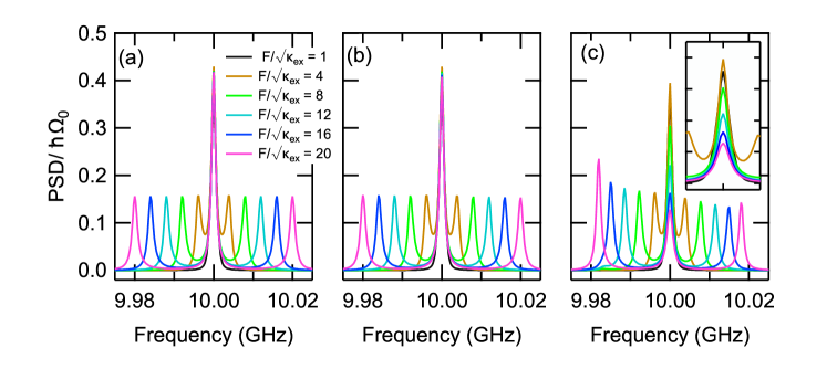
Figure 2:   Spectra of resonance fluorescence for (a) a two-level system, (b) a nonlinear resonator in the transmon regime ($K/2\pi=-200$ MHz) and (c) a nonlinear resonator in the KNR regime ($K/2\pi=-20$ MHz). Other parameters used in the calculation are $\Omega_{0}/2\pi=10$ GHz, $\kappa_{\rm ex}=\kappa_{\rm in}=2\pi\times 0.5$ MHz, and $\gamma_{\rm p}/2\pi=0.1$ MHz.

II.2 Numerical results

Figure 2 shows the numerical results of the resonance fluorescence spectra with varied drive amplitude $F$ for three systems: (a) a two-level system (TLS), (b) a nonlinear resonator with $K/2\pi=-200$ MHz (transmon) and (c) a nonlinear resonator with $K/2\pi=-20$ MHz (KNR). We assumed the dephasing rate of $\gamma_{\rm p}/2\pi$=0.1 MHz besides the external and internal loss rates of $\kappa_{\rm ex,in}/2\pi$=0.5 MHz. The spectra for the TLS and transmon [Figs. 2(a) and 2(b)] look almost identical and exhibit a typical Mollow triplet consisting of a center peak and symmetric sideband peaks. As the theory predicts Mollow (1969), when $|F|^{2}$ is much larger than decay rates, the height of these peaks are almost independent of $F$, and the position of the sideband peaks linearly depend on $F$. Since the Rabi frequency is much smaller than the Kerr nonlinearity, the transmon is in the weak-drive regime in the calculated range of $F$ and can be well approximated as a two-level system.

The spectra for the KNR [Fig. 2(c)] looks different and exhibit several distinct features. First, the heights of the sideband peaks are not symmetric: the lower sideband is higher than the upper sideband. Note that here we consider the resonant drive, namely, $\omega_{\rm d}=\Omega_{0}$. Asymmetric side peaks in fluorescence spectrum have been reported both in theory Koshino and Nakamura (2012) and experiment Lu et al. (2021), but they are under an off-resonant drive. Second, as shown in the inset of Fig. 2(c), the height of the center peak decreases significantly as $F$ increases. Third, the position of the sideband peaks is slightly different from those of the TLS and transmon, especially at large $F$, indicating the nonlinear dependence of the Rabi frequency on the drive strength Baur et al. (2009). Since the Rabi frequency is comparable to the Kerr nonlinearity, KNR is in the strong-drive regime for this range of $F$.

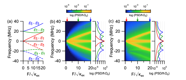
Figure 3:   (a) Transition frequencies between the dressed states as a function of the drive amplitude $F$ normalized by $\sqrt{\kappa_{\rm ex}}$. (b) and (c) Resonance fluorescence spectra of the nonlinear resonator in the KNR regime as a function of the frequency and $F/\sqrt{\kappa_{\rm ex}}$. We set the dephasing rate $\gamma_{\rm p}/2\pi$=0 in (b) and 0.1 MHz in (c). Other parameters used in the calculation are the same as those in Fig. 2(c). The frequency is measured from $\Omega_{0}/2\pi=10$ GHz. The right panels show the cross section of the left panels at the three values of $F/\sqrt{\kappa_{\rm ex}}$ indicated by the arrows.

To further study the spectra of the KNR, we investigate the effect of dephasing. Figures 3(b) and 3(c) show the resonance fluorescence spectra of a KNR calculated without and with the dephasing of $\gamma_{\rm p}/2\pi$=0.1 MHz, respectively. Other parameters used in the calculation are the same as those in Fig. 2(c). As seen in Fig. 3(b), the asymmetry in the spectrum disappears when there is no dephasing. We also plot in Fig. 3(a) the transition frequencies between the dressed states as a function of $F$. The label in the figure $E_{\tilde{i}}-E_{\tilde{j}}$ represents the energy difference between $i$th and $j$th eigenstates, which are obtained by diagonalizing the following Hamiltonian under a frame rotating at $\omega_{\rm d}=\Omega_{0}$:

$$~\mathcal{H}=\frac{K}{2}a^{\dagger}a^{\dagger}aa+\sqrt{\kappa_{\rm ex}}\,(F^{*}a+Fa^{\dagger}).$$ (21)

By comparing the figure with the spectra, we see that the peaks in Figs. 3(b) and 3(c) are observed at the transition frequencies between the dressed states. Especially, we observe more peaks than in the case of a TLS, namely, the Mollow triplet. They are conspicuous in the lower frequency range of Fig. 3(c) and attributed to the transitions from the second excited state.

To obtain insight into these characteristics, we adopt the notion that the peak intensity in the fluorescence is given by the product of the population of the initial state and the transition-matrix element between the initial and final states of the corresponding transition Lu et al. (2021). From Eq. (51), the total spectrum intensity is given by

$$~~\int\!d\omega\,S_{\rm i}(\omega) \propto \langle a^{\dagger}a\rangle_{\rm s}-|\langle a\rangle_{\rm s}|^{2}$$ (22)

$$\approx \sum_{i,j}P_{i}|\langle\tilde{j}|a|\tilde{i}\rangle|^{2}-|\langle a\rangle_{\rm s}|^{2},$$

where $P_{i}$ represents the population of the dressed state $|\tilde{i}\rangle$. Note that $P_{i}$ is a diagonal element of the density matrix. The last expression in Eq. (22) neglects contribution from the nondiagonal elements. Those are, however, negligibly smaller than the diagonal ones as we observe in Figs. 4(b) and 4(c) in the regime of $|F|^{2}>\kappa_{\rm ex}$.

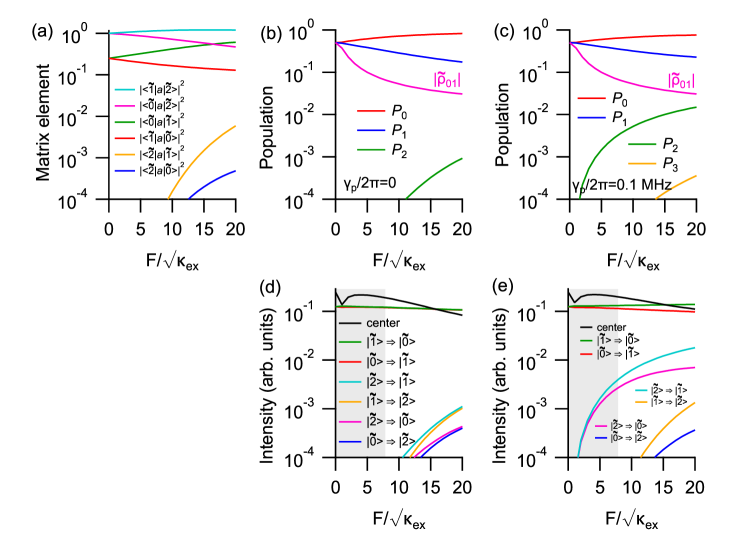
Figure 4:   (a) Squared transition-matrix elements $|\langle\tilde{j}|a|\tilde{i}\rangle|^{2}$ between the dressed states of the KNR. Eigenvectors are calculated by diagonalizing the Hamiltonian in Eq. (21). (b) and (c) Steady-state populations of the eigenstates, $P_{i}$, of the KNR for $\gamma_{\rm p}/2\pi=0$ and 0.1 MHz, respectively. Other parameters used in the calculation are the same as those in Fig. 2(c). Absolute value of the (0,1) component of the density matrix $|\tilde{\rho}_{01}|$ is also plotted. (d) and (e) Estimate of the fluorescence peak intensity from the product of $P_{i}$ and $|\langle\tilde{j}|a|\tilde{i}\rangle|^{2}$ for $\gamma_{\rm p}/2\pi=0$ and 0.1 MHz, respectively. The center-peak intensity (black line) is calculated with Eq. (23). The gray areas indicate the region where the off-diagonal components of the density matrix are non-negligible [$|\tilde{\rho}_{01}|$ larger than 10% of max($|\tilde{\rho}_{00}|$, $|\tilde{\rho}_{11}|$)] and therefore estimation based on Eq. (22) becomes unreliable.

Figure 4(a) shows the transition-matrix elements between the dressed states as a function of $F/\sqrt{\kappa_{\rm ex}}$. They are calculated using the eigenvectors of the Hamiltonian Eq. (21). Figures 4(b) and 4(c) show the population of the dressed states when $\gamma_{\rm p}/2\pi=0$ and 0.1 MHz, respectively. The population is calculated from $\langle\alpha_{m,n}\rangle_{\rm s}$ in Eq. (15) using the relation in Appendix B. As seen in the figures, dephasing enhances the population of higher levels. We also plot the absolute value of the (0,1) component of the density matrix $|\tilde{\rho}_{01}|$ calculated with Eq. (95). It is confirmed that they are much smaller than the dominant populations $P_{0}$ and $P_{1}$ when $F$ is sufficiently larger than $\sqrt{\kappa_{\rm ex}}$. Figures 4(d) and 4(e) show the product of the population $P_{i}$ and the transition matrix element $|\langle\tilde{j}|a|\tilde{i}\rangle|^{2}$, which is expected to represent the intensity of the fluorescence peak corresponding to the transition from $|\tilde{i}\rangle$ to $|\tilde{j}\rangle$. Also plotted in Figs. 4(c) and 4(d) in black lines are the intensity of the center peak, which is obtained by

$$~\sum_{i}P_{i}|\langle\tilde{i}|a|\tilde{i}\rangle|^{2}-|\langle a\rangle_{\rm s}|^{2}.$$ (23)

As seen from Fig. 4(d), the intensities of the paired sidebands of $|\tilde{1}\rangle\rightarrow|\tilde{0}\rangle$ and $|\tilde{0}\rangle\rightarrow|\tilde{1}\rangle$ are almost equal and independent of $F$ in this range, which is consistent with the result in Fig. 3(b). From Figs. 4(a) and 4(b), it is seen that this fact originates in the balance of the population and the transition matrix element. Namely, the increase in $P_{0}$ is compensated by the decrease in $|\langle\tilde{1}|a|\tilde{0}\rangle|^{2}$, and the decrease in $P_{1}$ is compensated by the increase in $|\langle\tilde{0}|a|\tilde{1}\rangle|^{2}$. It is also worth mentioning that intensities of other pairs of sideband (e.g., $|\tilde{2}\rangle\rightarrow|\tilde{1}\rangle$ and $|\tilde{1}\rangle\rightarrow|\tilde{2}\rangle$) are almost equal and are thus symmetric.

In the presence of dephasing ($\gamma_{\rm p}/2\pi=0.1$ MHz), we see in Fig. 4(c) that the populations of the excited states increase. This breaks the balance realized in the case without dephasing. As seen in Fig. 4(e), the intensity of the peak corresponding $|\tilde{1}\rangle\rightarrow|\tilde{0}\rangle$ ($|\tilde{0}\rangle\rightarrow|\tilde{1}\rangle$) increases (decreases) as a function of $F$. Also, intensities of other pairs of sideband are not equal and the intensity of the lower sideband peak is higher than the higher sideband peak (e.g., $|\tilde{2}\rangle\rightarrow|\tilde{1}\rangle$ is higer than $|\tilde{1}\rangle\rightarrow|\tilde{2}\rangle$). These are consistent with what is observed in Fig. 3(c).

More intuitively, the asymmetry of the sideband-peak intensity in the presence of dephasing can be understood in the following way. In general, dephasing in material quantum systems turns imaginary excitations to real excitations and accordingly makes their fluorescence spectra closer to the spontaneous-emission spectra Koshino (2011). In a KNR, because of the negative Kerr nonlinearity ($K<0$), the higher transition frequencies ($|j\rangle$ and $|j+1\rangle$ for $j\geq 1$) are smaller than the lowest transition frequency $\Omega_{0}$ ($|0\rangle$ and $|1\rangle$), so the spontaneous-emission spectrum from a highly-excited state would have a peak at a frequency lower than $\Omega_{0}$. Therefore, in the present situation where a KNR is driven by a resonant drive field at $\Omega_{0}$, the lower sideband of the Mollow triplet is more enhanced than the higher one. This intuitive understanding is supported by our numerical simulation (data not shown), where the higher sideband becomes more enhanced than the lower one when we assume a positive Kerr nonlinearity ($K>0$).

As for the center peak, the intensity decreases with $F/\sqrt{\kappa_{\rm ex}}\gtrsim 5$ regardless of the dephasing. This is consistent with the results in Figs. 2(c), 3(b) and 3(c), although it is less clear in the latter two. Intuitively, a KNR, due to its weak nonlinearity, becomes more like a harmonic oscillator at higher drive strength, which does not have incoherent scattering. The decrease in the intensity of the center peak is attributable to the energy transfer from the incoherent to coherent scatterings [Eqs. (11) and (10)]. Note that the finite intensity including the increase of the center peak at $F\rightarrow 0$ in Figs. 4(d) and 4(e) is due to the breakdown of the approximation in Eq. (22). Ideally, all the peaks should vanish at $F\rightarrow 0$.

III Experiments

To compare the above theory with experiments, we measure the fluorescence spectra in the strong-drive regime using a KNR with the Kerr nonlinearity of about 10 MHz. The KNR device used in the experiment is a type of frequency-tunable Xmon Barends et al. (2013) with the same design as the one reported in Ref. Yamaguchi et al. (2024), which consists of niobium electrodes sputtered and patterned on a silicon substrate and shadow-evaporated Josephson junctions made of aluminum. The KNR is capacitively coupled to the open end of a transmission line. In the present paper, we fix the magnetic flux bias of the KNR at zero.

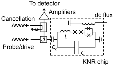
Figure 5:   Simplified experimental setup. The KNR consists of an asymmetric SQUID in series with two Josephson junctions and a line with the geometrical inductance $L$, which are in parallel with a shunt capacitor with the capacitance $C$. The KNR is coupled to a semi-infinite transmission line via a coupling capacitor with the capacitance $C_{\rm c}$ in a reflection-type configuration, where the input and output fields are separated by a circulator. A cancellation filed is injected through a directional coupler. The amplifiers include an IMPA at 10 mK, a HEMT at 4 K and another at room temperature.

Figure 5 shows the simplified experimental setup for our measurements (See Appendix C for the detailed one). The KNR is placed at the mixing-chamber stage of a dilution refrigerator at approximately 10 mK. For the measurement of reflection coefficients, we use a vector network analyzer. For the measurement of fluorescence spectra, a drive field is generated by a signal generator at room temperature and injected into the KNR. Fluorescence spectra from the KNR are measured using a spectrum analyzer with a resolution bandwidth of 10 kHz. To improve the measurement signal-to-noise ratio (SNR), we repeatedly turn on and off the drive field to obtain their difference. Each scan is averaged for 10 times, and this process is repeated for 200 times. We also used an impedance-matched Josephson parametric amplifier (IMPA) Urade et al. (2021) for the detection of the fluorescence signal. The input 1-dB compression point of the IMPA is around $-110$ dBm. To avoid saturating IMPA by the reflected drive field, a cancellation field is injected through a directional coupler. Any reflection signal that could not be completely suppressed by this cancellation field was removed during the data analysis.

Figure 6(a) shows the frequency dependence of the reflection coefficient $\Gamma$ of the KNR biased at zero magnetic field, which is measured with a weak probe power $P_{\rm p}$ of $-160.5$ dBm. Throughout the paper, the powers of the various tones are specified at the sample chip, which is calibrated by the method described below. By fitting the data with

$$\Gamma=1-\frac{\kappa_{\rm ex}}{\mathrm{i}(\omega_{\rm p}-\Omega_{0})+\frac{\kappa_{\rm ex}+\kappa_{\rm in}^{*}}{2}},$$ (24)

we obtain $\Omega_{0}/2\pi=10.3653$ GHz, $\kappa_{\rm ex}/2\pi=0.260\pm 0.002$ MHz, and $\kappa_{\rm in}^{*}/2\pi=0.053\pm 0.004$ MHz, after averaging 13 such measurements, where the errors are the standard deviations. Here, $\kappa_{\rm in}^{*}$ represents the nominal internal loss rate obtained from the reflection coefficient, which is the sum of the actual internal loss rate and the twice of the pure dephasing rate $\gamma_{\rm p}$, i.e., $\kappa_{\rm in}^{*}=\kappa_{\rm in}+2\gamma_{\rm p}$ Yamaguchi et al. (2024).

Figure 6(b) shows the result of the two-tone spectroscopy, in which the reflection coefficient is measured under the application of an additional drive field at $\omega_{\rm d}=\Omega_{0}$ with varying powers $P_{\rm d}$s. This measurement reveals the energy spectrum of the dressed states formed by the KNR and the drive field Yamaji et al. (2022). At weak drive powers, we observe two $P_{\rm d}$-independent dips one of which is located at $\omega_{\rm p}=\Omega_{0}$. The other one corresponds to the $|1\rangle$ to $|2\rangle$ transition of the bare KNR states and their separation gives the Kerr nonlinearity, which is determined to be $-9.7$ MHz as shown in the inset.

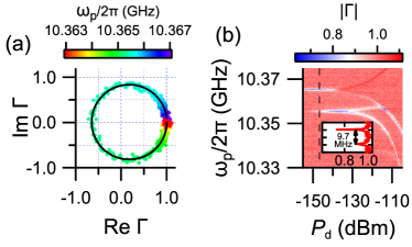
Figure 6:   (a) Reflection coefficient $\Gamma$ of the KNR biased at zero magnetic field as a function of the probe frequency $\omega_{\rm p}$ plotted in an IQ plane. The power of the probe field is $-160.5$ dBm. The dots represent the experimental data, while the black line represents the fitting. (b) Two-tone spectroscopy, where $|\Gamma|$ is plotted as a function of $\omega_{\rm p}$ (vertical axis) under the application of an additional drive field at $\omega_{\rm d}=\Omega_{0}$ with varying power $P_{\rm d}$ (horizontal axis). The power of the probe field is $-140.5$ dBm. The inset shows a cross-sectional view along the dotted line. The frequency separation between the two dips corresponds to the Kerr nonlinearity, which is $K/2\pi=-9.7$ MHz.

In order to determine the power of the fluorescence at the chip, we need to precisely determine the total amplification in the output line from the KNR chip to the detector at the room temperature. For that purpose, we calibrate the attenuation in the input line from the room temperature generator to the KNR chip by measuring the probe-power dependence of $\Gamma$ [Fig. 7(a)]. Because we know the total attenuation of the measurement line consisting of input and output lines from $|\Gamma|$ off the resonance frequency [background amplitude of $|\Gamma|$ in Fig. 7(a)], they allow us to determine the amplification in the output line.

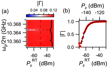
Figure 7:   (a) Probe-power dependence of the reflection coefficient. $|\Gamma|$ is plotted as a function of the probe frequency $\omega_{\rm p}$ (vertical axis) and the probe power at room temperature $P_{\rm p}^{\rm RT}$ (horizontal axis). The horizontal dashed line represents $\omega_{\rm p}=\Omega_{0}$. The black curve represents the cross-section along the vertical dashed line, where the horizontal amplitude shows $|\Gamma|$ in a linearly ascending unit. (b) Probe-power dependence of $|\Gamma|$ at $\omega_{\rm p}=\Omega_{0}$. The red dots represent the experimental data, which is the normalized cross-section along the horizontal dashed line in (a) plotted in the bottom axis, while the black line represents the theoretical curve Yamaji et al. (2022) plotted as a function of $P_{\rm p}$ in the top axis. In the calculation, we used $\Omega_{0}$, $\kappa_{\rm ex}$ and $\kappa_{\rm in}^{*}$ obtained from the measurement of $\Gamma$, and $K$ obtained from two-tone spectroscopy. From the difference between $P_{\rm p}^{\rm RT}$ and $P_{\rm p}$, we determine the attenuation of $-80.5$ dB in the input line.

Figure 7(a) shows $|\Gamma|$ as a function of $\omega_{\rm p}$ (vertical axis) and $P_{\rm p}^{\rm RT}$ (horizontal axis), where $P_{\rm p}^{\rm RT}$ is the power of the probe field represented by the value at the output of the network analyzer. As we increase $P_{\rm p}^{\rm RT}$, the dip observed at $\omega_{\rm p}=\Omega_{0}$ becomes shallower, and another dip at $\omega_{\rm p}=\Omega_{0}-K/2$ corresponding to the two-photon transition from $|0\rangle$ to $|2\rangle$ states appears at around $P_{\rm p}^{\rm RT}=-50$ dB (vertical dashed line). By comparing $|\Gamma|$ at $\omega_{\rm p}=\Omega_{0}$ with the theory based on the input–output formalism Yamaji et al. (2022) using experimentally determined parameters of $K$, $\kappa_{\rm ex}$ and $\kappa_{\rm in}$ as shown in Fig. 7(b), we determine the attenuation in the input line to be $-80.5$ dB. Note that in the calculation, we set $\kappa_{\rm in}=\kappa_{\rm in}^{*}$, namely, $\gamma_{\rm p}=0$. We confirmed that the result hardly depends on $\gamma_{\rm p}$ at least in a range relevant to the present study. From the total attenuation of $-18.9$ dB and taking into account the small difference in the attenuation between the setups for the measurement using network analyzer and spectrum analyzer, the gain in the output line is determined to be 61.0 dB. We also obtained consistent value in another calibration method based on the $P_{\rm d}$-dependence of the sideband-peak frequencies in the fluorescence spectra. Using this gain and that of the IMPA measured independently, we determine the amplitude of the measured spectra shown below.

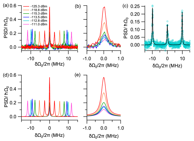
Figure 8:   (a) Resonance fluorescence spectra of a KNR at various drive powers. The resonance frequency of the KNR is 10.365 GHz. (b) Magnified view of (a) around the center peak. (c) Resonance fluorescence spectrum at $P_{\rm d}=-112.8$ dBm. The circles represent the experimental data, and the black line represents a theoretical fit to the data. (d) Calculated spectra using the parameters obtained from the fitting in (c) at the drive powers corresponding to the data in (a). (e) Magnified view of (d) around the center peak.

Figure 8 shows the fluorescence spectra measured at different $P_{\rm d}$’s. Similar to the case of two-level systems, we observe one center peak at $\Omega_{0}$ and two sideband peaks, whose separation (Rabi frequency) increases with $P_{\rm d}$. Additional subpeaks due to higer energy states were not observed probably due the limited SNR. Particularly noteworthy is the clear decrease of the center-peak intensity with $P_{\rm d}$ as shown in Fig. 8(b). This is one of the characteristic features of the strong-drive regime as we saw in Section II. Although the asymmetry of the sideband-peak intensities is another characteristic feature of the strong-drive regime, it is not so pronounced because the KNR is biased at the zero flux, where the pure dephasing rate is minimal. We pick up the data at $P_{\rm d}=-18.0$ dBm, where the Rabi frequency is close to $K$ and the large asymmetry in the sideband-peak intensities is expected in theory [Fig. 2(c)], and fitted it with the theory [Eq. (18)] as shown in Fig. 8(c). In the fitting, we used $\Omega_{0}$, $K$, $\kappa_{\rm ex}$ and the drive strength $F$ as fixed parameters, which are determined from the experiments and the calibration, and we used the internal loss rate $\kappa_{\rm in}$, and the pure dephasing rate $\gamma_{\rm p}$ as fitting parameters. In addition, we introduced another fitting parameter $A$, the overall scaling factor to account for the small error in the calibration of the amplification factor in the output line. We used the python package Optuna Akiba et al. (2019) for the fitting. We set the range of fitting parameters as $0\leq\kappa_{\rm in}\leq 2\pi\times 0.07$ MHz, $0\leq\gamma_{\rm p}\leq 2\pi\times 0.01$ MHz and $0.7\leq A\leq 1.1$ and the number of evaluation trials as 500. As a result of the fitting, we obtained $\kappa_{\rm in}/2\pi=0.046$ MHz, $\gamma_{\rm p}/2\pi=0.0065$ MHz, and $A=0.83~(-0.8$ dB). Note that $\kappa_{\rm in}+2\gamma_{\rm p}=2\pi\times 0.059$ MHz, which is consistent with $\kappa_{\rm in}^{*}$ obtained from the measurement of $\Gamma$.

Using the parameters obtained from the fitting, we calculate the spectra based on Eq. (18) at different drive powers and plot them in Figs. 8(d) and (e). The overall behavior of the $P_{\rm d}$-dependence of the sideband peaks and the center peak agrees well with the experimental results in Figs. 8(a) and (b).

IV Conclusion

We have investigated the fluorescence spectrum of the driven KNR. First, we developed a general formalism of coherent and incoherent scatterings of an external drive field by a KNR. The incoherent scattering gives the fluorescence spectrum of the driven KNR. Using the theory, we showed that the fluorescence spectrum of the KNR shows characteristic features distinct from the two-level system in the strong-drive regime, where the KNR is driven strongly such that the Rabi frequency is comparable or larger than the Kerr nonlinearity. Those features include the appearance of additional subpeaks, where higher excited states of the KNR are involved, the decrease of the center-peak intensity as the drive power, and asymmetric intensity of the sideband peaks in the presence of dephasing. To gain insight on those features, we calculated the steady-state population of the initial dressed state and its transition matrix element to the final dressed state and showed that their product gives a good estimate of the relative intensity of the corresponding peaks in the fluorescence spectrum.

We experimentally measured the resonance fluorescence using a superconducting KNR in the strong-drive regime, where both the Kerr nonlinearity and the Rabi frequency are $\sim 10$ MHz. We confirmed the decrease of the center-peak intensity. The overall spectra at different drive powers are well reproduced by our theory.

Future study includes the similar experiment at non-zero flux bias point to investigate how the spectrum changes as a function of the flux bias, namely, the strength of the dephasing rate. It will help to understand the basic properties of the KNR, which is an interesting platform for the quantum information processing Goto (2016b, a); Puri et al. (2017b, a).

Appendix A Calculation of fluorescence spectrum

Here we show the detailed calculation of the fluorescence spectrum in a system shown in Fig. 1 in the main text. To be self-contained, we also show the calculation of the fluorescence spectrum for the ideal two-level system, although it can be found in previous reports Koshino and Nakamura (2012); Lu et al. (2021).

A.1 Kerr nonlinear resonator

We consider the Hamiltonian Eq. (2) in the main text. From the Heisenberg equations of motion for $b_{k}$, we obtain

$$\frac{d}{dt}b_{k}(t)=-\mathrm{i}vkb_{k}(t)-\mathrm{i}\sqrt{\frac{v\kappa_{\rm ex}}{2\pi}}\,a(t).$$ (25)

By formally solving this differential equation, we have

$$b_{k}(t)=e^{-\mathrm{i}vkt}b_{k}(0)-\mathrm{i}\sqrt{\frac{v\kappa_{\rm ex}}{2\pi}}\int_{0}^{t}\!dt^{\prime}\,e^{-\mathrm{i}vk(t-t^{\prime})}a(t^{\prime}).$$ (26)

We introduce the real-space representation of the waveguide field as

$$\widetilde{b}_{r}=\frac{1}{\sqrt{2\pi}}\int\!dk\,e^{\mathrm{i}kr}b_{k}.$$ (27)

Note that $\bigl{[}\widetilde{b}_{r},\widetilde{b}^{\dagger}_{r^{\prime}}\bigr{]}=\delta(r-r^{\prime})$. In this representation, the waveguide field interacts with the resonator at $r=0$, and the $r<0$ ($r>0$) region corresponds to the incoming (outgoing) field. From Eq. (26), we have

$$~\widetilde{b}_{r}(t) = \frac{1}{\sqrt{2\pi}}\int\!dk\,e^{\mathrm{i}k(r-vt)}b_{k}(0)-\mathrm{i}\frac{\sqrt{v\kappa_{\rm ex}}}{2\pi}\int^{t}_{0}\!dt^{\prime}\int\!dk\,e^{\mathrm{i}k[r-v(t-t^{\prime})]}a(t^{\prime})$$

$$= \widetilde{b}_{r-vt}(0)-\mathrm{i}\sqrt{v\kappa_{\rm ex}}\int^{t}_{0}\!dt^{\prime}\,\delta[r-v(t-t^{\prime})]a(t^{\prime})$$

$$= \widetilde{b}_{r-vt}(0)-\mathrm{i}\sqrt{\frac{\kappa_{\rm ex}}{v}}\int^{t}_{0}\!dt^{\prime}\,\delta(t^{\prime}-t+r/v)a(t^{\prime})$$ (28)

$$= \widetilde{b}_{r-vt}(0)-\mathrm{i}\sqrt{\frac{\kappa_{\rm ex}}{v}}\,\theta(r)\theta(t-r/v)a(t-r/v),$$

where $\theta(r)$ is the Heaviside step function. We define the input and output operators as

$$b_{\rm in}(t) \equiv \widetilde{b}_{-0}(t)=\widetilde{b}_{-vt}(0),$$ (29)

$$b_{\rm out}(t) \equiv \widetilde{b}_{+0}(t)=b_{\rm in}(t)-\mathrm{i}\sqrt{\frac{\kappa_{\rm ex}}{v}}\,a(t).$$ (30)

Using Eqs. (28) and (29), the field operator $\widetilde{b}_{r}(t)$ at the resonator position ($r=0$) is given by

$$\widetilde{b}_{0}(t)=\frac{1}{\sqrt{2\pi}}\int\!dk\,b_{k}(t)=b_{\rm in}(t)-\frac{\mathrm{i}}{2}\sqrt{\frac{\kappa_{\rm ex}}{v}}\,a(t).$$ (31)

Similarly, from the Heisenberg equations of motion for $d_{k}$, we obtain

$$\frac{d}{dt}d_{k}(t)=-\mathrm{i}vkd_{k}(t)-\mathrm{i}\sqrt{\frac{v\gamma_{\rm p}}{\pi}}\,a^{\dagger}(t)a(t),$$ (32)

and

$$d_{k}(t)=e^{-\mathrm{i}vkt}d_{k}(0)-\mathrm{i}\sqrt{\frac{v\gamma_{\rm p}}{\pi}}\int_{0}^{t}\!dt^{\prime}\,e^{-\mathrm{i}vk(t-t^{\prime})}a^{\dagger}(t^{\prime})a(t^{\prime}).$$ (33)

The field operator $\widetilde{d}_{r}(t)$ at the resonator position ($r=0$) is given by

$$\widetilde{d}_{0}(t)=\frac{1}{\sqrt{2\pi}}\int\!dk\,d_{k}(t)=d_{\rm in}(t)-\mathrm{i}\sqrt{\frac{\gamma_{\rm p}}{2v}}\,a^{\dagger}(t)a(t).$$ (34)

From the Heisenberg equations of motion for $a$, we then obtain

$$~\frac{da}{dt} = \mathrm{i}[\mathcal{H}_{\rm sys}(t)/\hbar,a]+\mathrm{i}\sqrt{v\kappa_{\rm ex}}\,[a^{\dagger},a]\widetilde{b}_{0}+\mathrm{i}\sqrt{v\kappa_{\rm in}}\,[a^{\dagger},a]\widetilde{c}_{0}+\mathrm{i}\sqrt{2v\gamma_{\rm p}}\,\Bigl{(}[a^{\dagger}a,a]\widetilde{d}_{0}+\widetilde{d}^{\dagger}_{0}[a^{\dagger}a,a]\Bigr{)}$$ (35)

$$= \mathrm{i}[\mathcal{H}_{\rm sys}(t)/\hbar,a]-\mathrm{i}\sqrt{v\kappa_{\rm ex}}\,\widetilde{b}_{0}-\mathrm{i}\sqrt{v\kappa_{\rm in}}\,\widetilde{c}_{0}-\mathrm{i}\sqrt{2v\gamma_{\rm p}}\,(a\widetilde{d}_{0}+\widetilde{d}^{\dagger}_{0}a),$$

where we used $[a^{\dagger}a,a]=-a$. Using Eq. (31) and its counterparts for $\widetilde{c}_{0}$ and $\widetilde{d}_{0}$, Eq. (35) is rewritten as

$$~\frac{da}{dt} = \mathrm{i}[\mathcal{H}_{\rm sys}(t)/\hbar,a]-\frac{\kappa_{\rm ex}+\kappa_{\rm in}}{2}a+\gamma_{\rm p}[a^{\dagger}a,a]-\mathrm{i}\sqrt{v\kappa_{\rm ex}}\,b_{\rm in}(t)-\mathrm{i}\sqrt{v\kappa_{\rm in}}\,c_{\rm in}(t)$$

$$-\mathrm{i}\sqrt{2v\gamma_{\rm p}}\,[ad_{\rm in}(t)+d^{\dagger}_{\rm in}(t)a]$$

$$= -\Big{(}\mathrm{i}\Omega_{0}+\mathrm{i}Ka^{\dagger}a+\frac{\kappa}{2}\Bigr{)}a-\mathrm{i}\sqrt{v\kappa_{\rm ex}}\,b_{\rm in}(t)-\mathrm{i}\sqrt{v\kappa_{\rm in}}\,c_{\rm in}(t)$$ (36)

$$-\mathrm{i}\sqrt{2v\gamma_{\rm p}}\,[ad_{\rm in}(t)+d^{\dagger}_{\rm in}(t)a],$$

where $\kappa=\kappa_{\rm ex}+\kappa_{\rm in}+2\gamma_{\rm p}$ and we used $[a^{\dagger}a^{\dagger}aa,a]=-2a^{\dagger}aa$. We assume that at $t$=0, the system is in the vacuum and a drive field $\mathcal{F}(r/v-t)$ is injected from the external port, where

$$~\mathcal{F}(r/v-t)=Fe^{\mathrm{i}\omega_{\rm d}(r/v-t)}/\sqrt{v}.$$ (37)

The initial state vector is represented as

$$~|\psi(0)\rangle=\mathcal{N}\exp\Bigl{(}\int_{-\infty}^{0}\!dr\,\mathcal{F}(r/v)\widetilde{b}_{r}^{\dagger}(0)\Bigr{)}|{\rm v}\rangle,$$ (38)

where $|{\rm v}\rangle$ represents the ground state of the system, and $\mathcal{N}$ is a normalization constant. Note that $|\psi(0)\rangle$ is the eigenstate of $b_{\rm in}(t)$, namely,

$$~b_{\rm in}(t)|\psi(0)\rangle=\widetilde{b}_{-vt}(0)|\psi(0)\rangle=\mathcal{F}(-t)|\psi(0)\rangle.$$ (39)

Taking the expectation value of Eq. (36) with the initial state of the system $|\psi(0)\rangle$, we obtain

$$~\frac{d\langle a\rangle}{dt} = -\Big{(}\mathrm{i}\Omega_{0}+\frac{\kappa}{2}\Bigr{)}\langle a\rangle-\mathrm{i}K\langle a^{\dagger}aa\rangle-\mathrm{i}\sqrt{v\kappa_{\rm ex}}\,\langle b_{\rm in}(t)\rangle-\mathrm{i}\sqrt{v\kappa_{\rm in}}\,\langle c_{\rm in}(t)\rangle$$

$$-\mathrm{i}\sqrt{2v\gamma_{\rm p}}\,[\langle ad_{\rm in}(t)\rangle+\langle d^{\dagger}_{\rm in}(t)a\rangle]$$ (40)

$$= -\Big{(}\mathrm{i}\Omega_{0}+\frac{\kappa}{2}\Bigr{)}\langle a\rangle-\mathrm{i}K\langle a^{\dagger}aa\rangle-\mathrm{i}\sqrt{v\kappa_{\rm ex}}\,\langle b_{\rm in}(t)\rangle,$$

where we used $\langle c_{\rm in}(t)\rangle=0$, $d_{\rm in}(t)|\psi(0)\rangle=0$ and $\langle\psi(0)|d_{\rm in}^{\dagger}(t)=0$. As seen from Eq. (40), we cannot construct simultaneous equations of motion in a closed form. Thus we consider the equation of motion for $A_{m,n}\equiv{a^{\dagger}}^{m}a^{n}$ and numerically solve simultaneous equations of motion for finite $m$ and $n$. By using relations such as $\bigl{[}a^{\dagger},a^{n}\bigr{]}=-na^{n-1}$ and $\bigl{[}{a^{\dagger}}^{2},a^{n}\bigr{]}=-n(n-1)a^{n-2}-2na^{\dagger}a^{n-1}$, the equation of motion for $A_{m,n}$ is given by.

$$\frac{dA_{m,n}(t)}{dt} = \Big{[}\mathrm{i}(m-n)\Omega_{0}+\mathrm{i}(m-n)(m+n-1)\frac{K}{2}-(n+m)\frac{\kappa_{\rm ex}+\kappa_{\rm in}}{2}-(m-n)^{2}\gamma_{\rm p}\Bigr{]}A_{m,n}(t)$$ (41)

$$+\mathrm{i}K(m-n)A_{m+1,n+1}(t)$$

$$-\mathrm{i}\sqrt{v\kappa_{\rm ex}}\,[nA_{m,n-1}(t)b_{\rm in}(t)-mb^{\dagger}_{\rm in}(t)A_{m-1,n}(t)]$$

$$-\mathrm{i}\sqrt{v\kappa_{\rm in}}\,[nA_{m,n-1}(t)c_{\rm in}(t)-mc^{\dagger}_{\rm in}(t)A_{m-1,n}(t)]$$

$$+\mathrm{i}\sqrt{2v\gamma_{\rm p}}\,(m-n)[A_{m,n}(t)d_{\rm in}(t)+d^{\dagger}_{\rm in}(t)A_{m,n}(t)].$$

We take the expectation value of both sides of Eq. (41) with $|\psi(0)\rangle$ and obtain

$$\frac{d\langle A_{m,n}(t)\rangle}{dt}=\epsilon_{m,n}\langle A_{m,n}(t)\rangle+\mathrm{i}K(m-n)\langle A_{m+1,n+1}(t)\rangle\\ ~-\mathrm{i}\sqrt{\kappa_{\rm ex}}\,[n\langle A_{m,n-1}(t)\rangle Fe^{-\mathrm{i}\omega_{\rm d}t}-m\langle A_{m-1,n}(t)\rangle F^{*}e^{\mathrm{i}\omega_{\rm d}t}],$$ (42)

where we define

$$\epsilon_{m,n}\equiv\mathrm{i}(m-n)\Omega_{0}+\mathrm{i}(m-n)(m+n-1)\frac{K}{2}-(m+n)\frac{\kappa_{\rm ex}+\kappa_{\rm in}}{2}-(m-n)^{2}\gamma_{\rm p}.$$ (43)

Assuming a steady state, we set $\langle A_{m,n}(t)\rangle$ as

$$~\langle A_{m,n}(t)\rangle=\langle\alpha_{m,n}\rangle_{\rm s}e^{\mathrm{i}(m-n)\omega_{\rm d}t}$$ (44)

and substitute it into Eq. (42), which leads to

$$~0=\frac{d}{dt}\langle\alpha_{m,n}\rangle_{\rm s}=\epsilon_{m,n}^{\prime}\langle\alpha_{m,n}\rangle_{\rm s}+\mathrm{i}K(m-n)\langle\alpha_{m+1,n+1}\rangle_{\rm s}-\mathrm{i}\sqrt{\kappa_{\rm ex}}\,[n\langle\alpha_{m,n-1}\rangle_{\rm s}F-m\langle\alpha_{m-1,n}\rangle_{\rm s}F^{*}],$$ (45)

where

$$\epsilon_{m,n}^{\prime}\equiv\epsilon_{m,n}-\mathrm{i}(m-n)\omega_{\rm d}=\mathrm{i}(m-n)(\Omega_{0}-\omega_{\rm d})+\mathrm{i}(m-n)(m+n-1)\frac{K}{2}-(m+n)\frac{\kappa_{\rm ex}+\kappa_{\rm in}}{2}-(m-n)^{2}\gamma_{\rm p}.$$ (46)

Therefore, $\langle\alpha_{m,n}\rangle_{\rm s}$ is obtained by numerically solving the above equations for $m,n=0,1,\cdots,N_{\rm max}$, except for $(m,n)=(0,0)$, where we set $\langle\alpha_{0,0}\rangle_{\rm s}=1$.

Next we consider the spectrum of the output field $b_{\rm out}(t)$. The spectrum is given by

$$~S(\omega)=\operatorname{Re}\int_{0}^{\infty}\!\frac{d\tau}{\pi}\,e^{\mathrm{i}\omega\tau}\langle b_{\rm out}^{\dagger}(t)b_{\rm out}(t+\tau)\rangle.$$ (47)

Using Eq. (30),

$$~\langle b_{\rm out}^{\dagger}(t)b_{\rm out}(t+\tau)\rangle = \Big{\langle}\big{[}b_{\rm in}^{\dagger}(t)+\mathrm{i}\sqrt{\frac{\kappa_{\rm ex}}{v}}\,a^{\dagger}(t)\big{]}\big{[}b_{\rm in}(t+\tau)-\mathrm{i}\sqrt{\frac{\kappa_{\rm ex}}{v}}\,a(t+\tau)\bigr{]}\Big{\rangle}$$

$$= \big{\langle}b_{\rm in}^{\dagger}(t)b_{\rm in}(t+\tau)\big{\rangle}+\mathrm{i}\sqrt{\frac{\kappa_{\rm ex}}{v}}\,\big{\langle}a^{\dagger}(t)b_{\rm in}(t+\tau)\big{\rangle}$$

$$-\mathrm{i}\sqrt{\frac{\kappa_{\rm ex}}{v}}\,\big{\langle}b_{\rm in}^{\dagger}(t)a(t+\tau)\big{\rangle}+\frac{\kappa_{\rm ex}}{v}\big{\langle}a^{\dagger}(t)a(t+\tau)\big{\rangle}$$

$$= \big{\langle}b_{\rm in}^{\dagger}(t)\big{\rangle}\big{\langle}b_{\rm in}(t+\tau)\big{\rangle}+\mathrm{i}\sqrt{\frac{\kappa_{\rm ex}}{v}}\,\big{\langle}a^{\dagger}(t)\big{\rangle}\big{\langle}b_{\rm in}(t+\tau)\big{\rangle}-\mathrm{i}\sqrt{\frac{\kappa_{\rm ex}}{v}}\,\big{\langle}b_{\rm in}^{\dagger}(t)\big{\rangle}\big{\langle}a(t+\tau)\big{\rangle}$$

$$+\frac{\kappa_{\rm ex}}{v}\big{\langle}a^{\dagger}(t)\big{\rangle}\big{\langle}a(t+\tau)\big{\rangle}+\frac{\kappa_{\rm ex}}{v}\big{\langle}a^{\dagger}(t),a(t+\tau)\big{\rangle}$$ (48)

$$= \langle b_{\rm out}^{\dagger}(t)\rangle\langle b_{\rm out}(t+\tau)\rangle+\frac{\kappa_{\rm ex}}{v}\big{\langle}a^{\dagger}(t),a(t+\tau)\big{\rangle},$$

where in the third equality, we used Eq. (39), and $\langle A,B\rangle=\langle AB\rangle-\langle A\rangle\langle B\rangle$. From Eqs. (47) and (48),

$$S(\omega) \equiv S_{\rm c}(\omega)+S_{\rm i}(\omega)$$ (49)

$$S_{\rm c}(\omega) = \operatorname{Re}\int_{0}^{\infty}\!\frac{d\tau}{\pi}\,e^{\mathrm{i}\omega\tau}\langle b_{\rm out}^{\dagger}(t)\rangle\langle b_{\rm out}(t+\tau)\rangle$$ (50)

$$S_{\rm i}(\omega) = \operatorname{Re}\int_{0}^{\infty}\!\frac{d\tau}{\pi}\,e^{\mathrm{i}\omega\tau}\frac{\kappa_{\rm ex}}{v}\langle a^{\dagger}(t),a(t+\tau)\rangle,$$ (51)

where $S_{\rm c}(\omega)$ and $S_{\rm i}(\omega)$ represent coherent and incoherent components, respectively.

First, we consider the incoherent component and define the following quantity.

$$B_{m,n}(t,\tau)\equiv\langle a^{\dagger}(t),A_{m,n}(t+\tau)\rangle.$$ (52)

The equation of motion for $B_{m,n}$ is given by

$$~\frac{d}{d\tau}B_{m,n}(t,\tau)=\epsilon_{m,n}B_{m,n}(t,\tau)+\mathrm{i}K(m-n)B_{m+1,n+1}(t,\tau)\\ -\mathrm{i}\sqrt{\kappa_{\rm ex}}\,[nB_{m,n-1}(t,\tau)Fe^{-\mathrm{i}\omega_{\rm d}(t+\tau)}-mB_{m-1,n}(t,\tau)F^{*}e^{\mathrm{i}\omega_{\rm d}(t+\tau)}].$$ (53)

Assuming a steady state, we set

$$B_{m,n}(t,\tau)=e^{\mathrm{i}(m-n)\omega_{\rm d}\tau}e^{\mathrm{i}(m-n+1)\omega_{\rm d}t}\beta_{m,n}(\tau),$$ (54)

and substitute it into Eq. (53) to obtain

$$~\frac{d}{d\tau}\beta_{m,n}=\epsilon_{m,n}^{\prime}\beta_{m,n}+\mathrm{i}K(m-n)\beta_{m+1,n+1}-\mathrm{i}\sqrt{\kappa_{\rm ex}}\,[n\beta_{m,n-1}F-m\beta_{m-1,n}F^{*}].$$ (55)

In order to solve this equation, we introduce Laplace transformation of $\beta_{m,n}$,

$$\overline{\beta_{m,n}}(s)\equiv\int_{0}^{\infty}\!d\tau\,e^{-s\tau}\beta_{m,n}(\tau).$$ (56)

By Laplace transforming both sides of Eq. (55),

$$~\beta_{m,n}(0)=(s-\epsilon_{m,n}^{\prime})\,\overline{\beta_{m,n}}(s)-\mathrm{i}K(m-n)\,\overline{\beta_{m+1,n+1}}(s)+\mathrm{i}\sqrt{\kappa_{\rm ex}}\,[n\,\overline{\beta_{m,n-1}}(s)F-m\,\overline{\beta_{m-1,n}}(s)F^{*}].$$ (57)

Here $\beta_{m,n}(0)$ can be calculated as

$$~\beta_{m,n}(0) = B_{m,n}(t,0)e^{-\mathrm{i}(m-n+1)\omega_{\rm d}t}$$

$$= \langle a^{\dagger}(t),A_{m,n}(t)\rangle e^{-\mathrm{i}(m-n+1)\omega_{\rm d}t}$$

$$= \Bigl{[}\langle A_{m+1,n}(t)\rangle-\langle A_{1,0}(t)\rangle\langle A_{m,n}(t)\rangle\Bigr{]}e^{-\mathrm{i}(m-n+1)\omega_{\rm d}t}$$ (58)

$$= \langle\alpha_{m+1,n}\rangle_{\rm s}-\langle\alpha_{1,0}\rangle_{\rm s}\langle\alpha_{m,n}\rangle_{\rm s},$$

where we used Eq. (44) in the last equality. Thus, in the steady state, Eq. (57) becomes

$$~\langle\alpha_{m+1,n}\rangle_{\rm s}-\langle\alpha_{1,0}\rangle_{\rm s}\langle\alpha_{m,n}\rangle_{\rm s}=(s-\epsilon’_{m,n})\,\overline{\beta_{m,n}}(s)-\mathrm{i}K(m-n)\,\overline{\beta_{m+1,n+1}}(s)\\ +\mathrm{i}\sqrt{\kappa_{\rm ex}}\,[n\,\overline{\beta_{m,n-1}}(s)F-m\,\overline{\beta_{m-1,n}}(s)F^{*}].$$ (59)

Using the solution of Eq. (45), we can numerically solve Eq. (59) for $m,n=0,1,\cdots,N_{\rm max}$, except for $\overline{\beta_{0,0}}(s)=0$. From Eq. (51),

$$~S_{\rm i}(\omega) = \operatorname{Re}\int_{0}^{\infty}\!\frac{d\tau}{\pi}\,e^{\mathrm{i}\omega\tau}\frac{\kappa_{\rm ex}}{v}\langle a^{\dagger}(t),a(t+\tau)\rangle$$

$$= \frac{\kappa_{\rm ex}}{\pi v}\operatorname{Re}\int_{0}^{\infty}\!d\tau\,e^{\mathrm{i}\omega\tau}B_{0,1}(t,\tau)$$ (60)

$$= \frac{\kappa_{\rm ex}}{\pi v}\operatorname{Re}\overline{\beta_{0,1}}\bigl{(}\mathrm{i}(\omega_{\rm d}-\omega)\bigr{)}~.$$

Next we consider the coherent component. In the steady state,

$$~\langle b_{\rm out}^{\dagger}(t)\rangle\langle b_{\rm out}(t+\tau)\rangle = \Big{\langle}b_{\rm in}^{\dagger}(t)+\mathrm{i}\sqrt{\frac{\kappa_{\rm ex}}{v}}\,a^{\dagger}(t)\Big{\rangle}\Big{\langle}b_{\rm in}(t+\tau)-\mathrm{i}\sqrt{\frac{\kappa_{\rm ex}}{v}}\,a(t+\tau)\Big{\rangle}$$

$$= \frac{e^{-\mathrm{i}\omega_{\rm d}\tau}}{v}(F-\mathrm{i}\sqrt{\kappa_{\rm ex}}\,\langle\alpha_{0,1}\rangle_{\rm s})(F^{*}+\mathrm{i}\sqrt{\kappa_{\rm ex}}\,\langle\alpha_{1,0}\rangle_{\rm s}).$$ (61)

$$= \frac{e^{-\mathrm{i}\omega_{\rm d}\tau}}{v}\Bigl{|}F-\mathrm{i}\sqrt{\kappa_{\rm ex}}\,\langle\alpha_{0,1}\rangle_{\rm s}\Bigr{|}^{2}.$$

From Eq. (50),

$$~S_{\rm c}(\omega) = \operatorname{Re}\int_{0}^{\infty}\!\frac{d\tau}{\pi}\,e^{\mathrm{i}\omega\tau}\langle b_{\rm out}^{\dagger}(t)\rangle\langle b_{\rm out}(t+\tau)\rangle$$ (62)

$$= \frac{\delta(\omega-\omega_{\rm d})}{v}\Bigl{|}F-\mathrm{i}\sqrt{\kappa_{\rm ex}}\,\langle\alpha_{0,1}\rangle_{\rm s}\Bigr{|}^{2}.~$$

A.2 Ideal two-level system

In this section, we consider the case where the Kerr nonlinear resonator in Fig. 1 is replaced by an ideal two-level system Koshino and Nakamura (2012); Lu et al. (2021). Namely,

$$~\mathcal{H}_{\rm sys}(t)/\hbar=\Omega_{0}\sigma^{\dagger}\sigma,$$ (63)

Similarly to the previous section, the equation of motion for $\sigma$ and $\sigma^{\dagger}\sigma$ is given by

$$~\frac{d\sigma}{dt} = -\Big{(}\mathrm{i}\Omega_{0}+\frac{\kappa}{2}\Bigr{)}\sigma-\mathrm{i}\sqrt{v\kappa_{\rm ex}}\,(1-2\sigma^{\dagger}\sigma)b_{\rm in}(t)-\mathrm{i}\sqrt{v\kappa_{\rm in}}\,(1-2\sigma^{\dagger}\sigma)c_{\rm in}(t)$$ (64)

$$-\mathrm{i}\sqrt{2v\gamma_{\rm p}}\,\bigl{[}\sigma d_{\rm in}(t)+d^{\dagger}_{\rm in}(t)\sigma\bigr{]},$$

$$~\frac{d}{dt}\sigma^{\dagger}\sigma = -(\kappa_{\rm ex}+\kappa_{\rm in})\sigma^{\dagger}\sigma+\mathrm{i}\sqrt{v\kappa_{\rm ex}}\,\bigl{[}b_{\rm in}^{\dagger}(t)\sigma-\sigma^{\dagger}b_{\rm in}(t)\bigr{]}$$ (65)

$$+\mathrm{i}\sqrt{v\kappa_{\rm in}}\,\bigl{[}c_{\rm in}^{\dagger}(t)\sigma-\sigma^{\dagger}c_{\rm in}(t)\bigr{]},$$

where we used $[\sigma,\sigma^{\dagger}]=1-\sigma^{\dagger}\sigma$ and $[\sigma^{\dagger}\sigma,\sigma]=-\sigma$. Taking the expectation value of $|\psi(0)\rangle$ on both sides, we get

$$~\frac{d\langle\sigma\rangle}{dt} = -\Big{(}\mathrm{i}\Omega_{0}+\frac{\kappa}{2}\Bigr{)}\langle\sigma\rangle-\mathrm{i}\sqrt{v\kappa_{\rm ex}}\,(1-2\langle\sigma^{\dagger}\sigma\rangle)\mathcal{F}(-t),$$ (66)

$$~\frac{d}{dt}\langle\sigma^{\dagger}\sigma\rangle = -(\kappa_{\rm ex}+\kappa_{\rm in})\langle\sigma^{\dagger}\sigma\rangle+\mathrm{i}\sqrt{v\kappa_{\rm ex}}\,\bigl{[}\mathcal{F}^{*}(-t)\langle\sigma\rangle-\mathcal{F}(-t)\langle\sigma\rangle^{*}\bigr{]}.$$ (67)

Note that in contrast to Eq. (40), Eqs. (66) and (67) form closed simultaneous equations. To obtain the steady-state solutions, we set

$$~\langle\sigma(t)\rangle = \langle\sigma\rangle_{\rm s}e^{-\mathrm{i}\omega_{\rm d}t},$$ (68)

$$~\langle\sigma^{\dagger}(t)\sigma(t)\rangle = \langle\sigma^{\dagger}\sigma\rangle_{\rm s}.$$ (69)

By substituting Eqs. (37), (68), and (69) into Eqs. (66) and (67), we obtain

$$~\langle\sigma\rangle_{\rm s} = \frac{-\mathrm{i}\sqrt{\kappa_{\rm ex}}\,\bigl{[}\kappa/2+\mathrm{i}(\omega_{\rm d}-\Omega_{0})\bigr{]}F}{2\overline{r}\kappa_{\rm ex}|F|^{2}+|\kappa/2+\mathrm{i}(\omega_{\rm d}-\Omega_{0})|^{2}}$$ (70)

$$~\langle\sigma^{\dagger}\sigma\rangle_{\rm s} = \frac{\overline{r}\kappa_{\rm ex}|F|^{2}}{2\overline{r}\kappa_{\rm ex}|F|^{2}+|\kappa/2+\mathrm{i}(\omega_{\rm d}-\Omega_{0})|^{2}},$$ (71)

where $\overline{r}=\kappa/(\kappa_{\rm ex}+\kappa_{\rm in})$.

As seen from Eq. (51), we need $\langle\sigma^{\dagger}(t),\sigma(t+\tau)\rangle$ to calculate the fluorescence, so that we define

$$B_{1}(t,\tau)\equiv\langle\sigma^{\dagger}(t),\sigma(t+\tau)\rangle$$ (72)

and consider its equation of motion. We find that by additionally defining

$$B_{2}(t,\tau) \equiv \langle\sigma^{\dagger}(t),\sigma^{\dagger}(t+\tau)\rangle$$ (73)

$$B_{3}(t,\tau) \equiv \langle\sigma^{\dagger}(t),\sigma^{\dagger}(t+\tau)\sigma(t+\tau)\rangle,$$ (74)

we obtain the simultaneous equations of motion in closed form as follows:

$$~\frac{\partial}{\partial\tau}B_{1}(t,\tau) = \Bigl{\langle}\sigma^{\dagger}(t)\frac{\partial}{\partial\tau}\sigma(t+\tau)\Bigr{\rangle}-\bigl{\langle}\sigma^{\dagger}(t)\bigr{\rangle}\Bigl{\langle}\frac{\partial}{\partial\tau}\sigma(t+\tau)\Bigr{\rangle}$$ (75)

$$= \Bigl{\langle}\sigma^{\dagger}(t)\Bigl{[}-\Big{(}\mathrm{i}\Omega_{0}+\frac{\kappa}{2}\Bigr{)}\sigma(t+\tau)-\mathrm{i}\sqrt{v\kappa_{\rm ex}}\,\bigl{[}1-2\sigma^{\dagger}(t+\tau)\sigma(t+\tau)\bigr{]}b_{\rm in}(t+\tau)\Bigr{]}\Bigr{\rangle}$$

$$-\bigl{\langle}\sigma^{\dagger}(t)\bigr{\rangle}\Bigl{\langle}-\Big{(}\mathrm{i}\Omega_{0}+\frac{\kappa}{2}\Bigr{)}\sigma(t+\tau)-\mathrm{i}\sqrt{v\kappa_{\rm ex}}\,\bigl{[}1-2\sigma^{\dagger}(t+\tau)\sigma(t+\tau)\bigr{]}b_{\rm in}(t+\tau)\Bigr{\rangle}$$

$$= -\Big{(}\mathrm{i}\Omega_{0}+\frac{\kappa}{2}\Bigr{)}B_{1}(t,\tau)+2\mathrm{i}\sqrt{v\kappa_{\rm ex}}\,\mathcal{F}[-(t+\tau)]B_{3}(t,\tau)$$

$$\frac{\partial}{\partial\tau}B_{2}(t,\tau) = \Big{(}\mathrm{i}\Omega_{0}-\frac{\kappa}{2}\Bigr{)}B_{2}(t,\tau)-2\mathrm{i}\sqrt{v\kappa_{\rm ex}}\,\mathcal{F}^{*}[-(t+\tau)]B_{3}(t,\tau)$$ (76)

$$\frac{\partial}{\partial\tau}B_{3}(t,\tau) = \mathrm{i}\sqrt{v\kappa_{\rm ex}}\,\mathcal{F}^{*}[-(t+\tau)]B_{1}(t,\tau)-\mathrm{i}\sqrt{v\kappa_{\rm ex}}\,\mathcal{F}[-(t+\tau)]B_{2}(t,\tau)$$ (77)

$$-(\kappa_{\rm ex}+\kappa_{\rm in})B_{3}(t,\tau),$$

where in Eq. (LABEL:B1_deriv), we used Eq. (64) and omitted terms containing $c_{\rm in}$ and $d_{\rm in}$, which will disappear in Eq. (75) after all. Assuming a steady state, we set

$$B_{1}(t,\tau) = e^{-\mathrm{i}\omega_{\rm d}\tau}\beta_{1}(\tau)$$ (78)

$$B_{2}(t,\tau) = e^{\mathrm{i}\omega_{\rm d}(2t+\tau)}\beta_{2}(\tau)$$ (79)

$$B_{3}(t,\tau) = e^{\mathrm{i}\omega_{\rm d}t}\beta_{3}(\tau),$$ (80)

and substitute them into the above equations with Eq. (37) and obtain

$$~\frac{d}{d\tau}\begin{bmatrix}\beta_{1}(\tau)\\ \beta_{2}(\tau)\\ \beta_{3}(\tau)\\ \end{bmatrix}=\begin{bmatrix}\mathrm{i}(\omega_{\rm d}-\Omega_{0})-\kappa/2&0&2\mathrm{i}\sqrt{\kappa_{\rm ex}}\,F\\ 0&-\mathrm{i}(\omega_{\rm d}-\Omega_{0})-\kappa/2&-2\mathrm{i}\sqrt{\kappa_{\rm ex}}\,F^{*}\\ \mathrm{i}\sqrt{\kappa_{\rm ex}}\,F^{*}&-\mathrm{i}\sqrt{\kappa_{\rm ex}}\,F&-(\kappa_{\rm ex}+\kappa_{\rm in})\\ \end{bmatrix}\begin{bmatrix}\beta_{1}(\tau)\\ \beta_{2}(\tau)\\ \beta_{3}(\tau)\\ \end{bmatrix}.$$ (82)

In order to solve this equation, we introduce Laplace transformation of $\beta_{i}(\tau)$ ($i$=1, 2 and 3),

$$\overline{\beta_{i}}(s)\equiv\int_{0}^{\infty}\!d\tau\,e^{-s\tau}\beta_{i}(\tau).$$ (83)

By Laplace transforming both sides of Eq. (82), we obtain

$$\begin{bmatrix}\beta_{1}(0)\\ \beta_{2}(0)\\ \beta_{3}(0)\\ \end{bmatrix}=\begin{bmatrix}s-\mathrm{i}(\omega_{\rm d}-\Omega_{0})+\kappa/2&0&-2\mathrm{i}\sqrt{\kappa_{\rm ex}}\,F\\ 0&s+\mathrm{i}(\omega_{\rm d}-\Omega_{0})+\kappa/2&2\mathrm{i}\sqrt{\kappa_{\rm ex}}\,F^{*}\\ -\mathrm{i}\sqrt{\kappa_{\rm ex}}\,F^{*}&\mathrm{i}\sqrt{\kappa_{\rm ex}}\,F&s+\kappa_{\rm ex}+\kappa_{\rm in}\\ \end{bmatrix}\begin{bmatrix}\overline{\beta_{1}}(s)\\ \overline{\beta_{2}}(s)\\ \overline{\beta_{3}}(s).\\ \end{bmatrix}$$ (84)

By noting that

$$\beta_{1}(0) = \langle\sigma^{\dagger}\sigma\rangle_{\rm s}-|\langle\sigma\rangle_{\rm s}|^{2}$$ (85)

$$\beta_{2}(0) = -(\langle\sigma\rangle_{\rm s}^{*})^{2}$$ (86)

$$\beta_{3}(0) = -\langle\sigma\rangle_{\rm s}^{*}\langle\sigma^{\dagger}\sigma\rangle_{\rm s},$$ (87)

where we used $\langle\sigma^{\dagger}(t)\sigma^{\dagger}(t)\rangle=0$, we obtain

$$~\begin{bmatrix}\overline{\beta_{1}}(s)\\ \overline{\beta_{2}}(s)\\ \overline{\beta_{3}}(s)\\ \end{bmatrix}=\begin{bmatrix}s-\mathrm{i}(\omega_{\rm d}-\Omega_{0})+\kappa/2&0&-2\mathrm{i}\sqrt{\kappa_{\rm ex}}\,F\\ 0&s+\mathrm{i}(\omega_{\rm d}-\Omega_{0})+\kappa/2&2\mathrm{i}\sqrt{\kappa_{\rm ex}}\,F^{*}\\ -\mathrm{i}\sqrt{\kappa_{\rm ex}}\,F^{*}&\mathrm{i}\sqrt{\kappa_{\rm ex}}\,F&s+\kappa_{\rm ex}+\kappa_{\rm in}\\ \end{bmatrix}^{-1}\begin{bmatrix}\langle\sigma^{\dagger}\sigma\rangle_{\rm s}-|\langle\sigma\rangle_{\rm s}|^{2}\\ -(\langle\sigma\rangle_{\rm s}^{*})^{2}\\ -\langle\sigma\rangle_{\rm s}^{*}\langle\sigma^{\dagger}\sigma\rangle_{\rm s}\\ \end{bmatrix}.$$ (88)

From Eq. (51),

$$~S_{\rm i}(\omega) = \operatorname{Re}\int_{0}^{\infty}\!\frac{d\tau}{\pi}\,e^{\mathrm{i}\omega\tau}\frac{\kappa_{\rm ex}}{v}\langle\sigma^{\dagger}(t),\sigma(t+\tau)\rangle$$ (89)

$$= \frac{\kappa_{\rm ex}}{\pi v}\operatorname{Re}\overline{\beta_{1}}\bigl{(}\mathrm{i}(\omega_{\rm d}-\omega)\bigr{)}.$$

By combining Eqs. (88) and (89), we can numerically calculate $S_{\rm i}(\omega)$. As for $S_{\rm c}(\omega)$, we can calculate it similarly to Eq. (62) as

$$S_{\rm c}(\omega)=\frac{\delta(\omega-\omega_{\rm d})}{v}\Bigl{|}F-\mathrm{i}\sqrt{\kappa_{\rm ex}}\,\langle\sigma\rangle_{\rm s}\Bigr{|}^{2},$$ (90)

where $\langle\sigma\rangle_{\rm s}$ is given in Eq. (70).

Appendix B Calculation of the dressed-state populations

In this Appendix, we derive the relation between the density matrix in eigenstate basis and $\langle\alpha_{m,n}\rangle_{\rm s}$ in Eq. (15) to calculate the population shown in Figs. 4(b) and 4(c). We denote the $m$th Fock state as $|m\rangle$ and the $i$th eigenstate of the Hamiltonian Eq. (21) as $|\tilde{i}\rangle$, which are related by a unitary matrix

$$U=\sum_{m,i}U_{mi}|m\rangle\langle\tilde{i}|.$$ (91)

Using

$$a^{n}=\sum_{k\geq 0}\sqrt{\frac{(k+n)!}{k!}}\,|k\rangle\langle k+n|,$$ (92)

$\langle\alpha_{m,n}\rangle_{\rm s}$ is calculated as

$$~\langle{a^{\dagger}}^{m}a^{n}\rangle_{\rm s} = \sum_{k\geq 0}\frac{\sqrt{(k+m)!(k+n)!}}{k!}\,\rho_{n+k,m+k}$$ (93)

$$= \sum_{k\geq 0}\frac{\sqrt{(k+m)!(k+n)!}}{k!}\,(U\tilde{\rho}U^{\dagger})_{n+k,m+k},~$$

where $\rho$ and $\tilde{\rho}$ represent the density matrices in the Fock-state and dressed-state bases, respectively. Introducing a diagonal and shifted-diagonal matrices of $D_{nm}=\sqrt{n!}\,\delta_{nm}$ and $A_{nm}=\delta_{n+1,m}$, Eq. (93) further leads

$$~\langle\alpha_{m,n}\rangle_{\rm s} = \frac{1}{k!}\sum_{k\geq 0}(DU\tilde{\rho}U^{\dagger}D)_{n+k,m+k}$$

$$= \frac{1}{k!}\sum_{k\geq 0}(A^{k}DU\tilde{\rho}U^{\dagger}D{A^{\dagger}}^{k})_{nm}$$ (94)

$$= (e^{\mathcal{A}}\cdot DU\tilde{\rho}U^{\dagger}D)_{nm},~$$

where $\mathcal{A}$ represents a linear mapping represented by $\mathcal{A}\cdot X\rightarrow AXA^{\dagger}$ for a matrix $X$. From Eq. (94),

$$~\tilde{\rho}_{ij} = [U^{\dagger}D^{-1}(e^{-\mathcal{A}}\cdot\alpha)D^{-1}U]_{ij}$$ (95)

$$= \sum_{m,n}\sum_{k\geq 0}\frac{(-1)^{k}}{k!\sqrt{n!m!}}U^{\dagger}_{im}\alpha_{n+k,m+k}U_{nj},~$$

where we defined a matrix $\alpha$ with elements given by $\alpha_{mn}=\langle{a^{\dagger}}^{m}a^{n}\rangle_{\rm s}$. From Eq. (95), we obtain the population of the eigenstate as

$$P_{i}=\tilde{\rho}_{ii}=\sum_{m,n}\sum_{k\geq 0}\frac{(-1)^{k}}{k!\sqrt{n!m!}}U^{\dagger}_{im}\alpha_{n+k,m+k}U_{ni}.$$ (96)

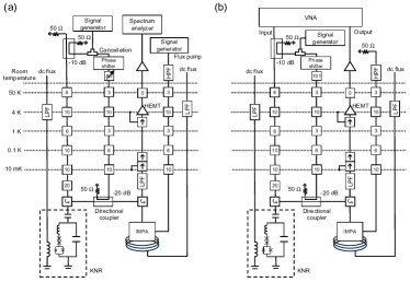
Figure 9:   Experimental setup for the measurement of (a) fluorescence (Fig. 8) and (b) reflection coefficient with and without drive field (Figs. 6 and 7).

Appendix C Detailed experimental setup

Figure 9 shows the detailed measurement setup used in the present study. For the fluorescence measurement (Fig. 8), we used the setup shown in Fig. 9(a), where a spectrum analyzer was used as the detector. For the reflection-coefficient measurements with and without a drive field (Figs. 6 and 7), we used the setup shown in Fig. 9(b), where a vector network analyzer (VNA) was used.

In the fluorescence measurement, we used a cancellation field in order to suppress the reflected drive field by the destructive interference and avoid saturating IMPA. To adjust the amplitude and phase of the cancellation field, we used a phase shifter and a variable attenuator, which are put in one of the two paths from the output of the signal generator split by the power divider. After the adjustment, we suppressed the power below $\sim-160$ dBm at the input of IMPA.

In the reflection-coefficient measurements (Figs. 6 and 7), we did not use IMPA. We turned off the pump and set the flux bias far detuned from the resonance frequency of KNR. Because the cancellation field is not necessary, we set the maximum attenuation of the variable attenuator (101 dB) and effectively turned it off.

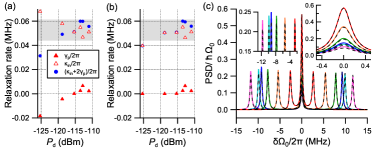
Figure 10:   Relaxation rates obtained by fitting the fluorescence spectra using (a) the fmin function and (b) Optuna. The gray region represents the two standard deviations of the mean of $\kappa_{\rm in}^{*}$ determined from the reflection-coefficient measurements. (c) Comparison of the spectra with and without the dephasing. Solid curves represent the same data as in Fig. 8(c), where $\gamma_{\rm p}/2\pi=0.0065$ MHz and $\kappa_{\rm in}/2\pi=0.046$ MHz, while the dashed curves represent those with $\gamma_{\rm p}$ and $\kappa_{\rm in}$ changed to zero and $2\pi\times 0.059$ MHz, respectively. The left upper inset shows the magnification of lower sideband peaks. The right upper inset shows the magnification of center peaks.

Appendix D Numerical fitting of the fluorescence data

In Fig. 8(c) in the main text, we showed the numerical fitting of the fluorescence data with $P_{\rm d}=-112.8$ dBm using a python package Optuna Akiba et al. (2019). We tried fitting the data with other $P_{\rm d}$’s with the same parameter setting. We also tried fitting using the fmin function in SciPy library with the initial guess of $A=1.0$, $\kappa_{\rm in}/2\pi=0.05$ MHz, and $\gamma_{\rm p}/2\pi=0.0025$ MHz. The obtained relaxation rates using the fmin function and Optuna as a function of $P_{\rm d}$ are plotted in Figs. 10(a) and (b), respectively. For $P_{\rm d}<-115$ dBm, we could not obtain reasonable value of $\gamma_{\rm p}$ in either method. They are either too small or even negative in the case of the fmin function, where no restriction in the parameter range was set. We suspect that this is because of the lower sensitivity of the spectrum to $\gamma_{\rm p}$ at lower $P_{\rm d}$’s. Figure 10(c) shows the comparison of the spectrum with and without the dephasing. Solid curves represent the same spectra as shown in Fig. 8(c), where $\gamma_{\rm p}/2\pi=0.0065$ MHz and $\kappa_{\rm in}/2\pi=0.046$ MHz, while the dashed curves represent those with $\gamma_{\rm p}/2\pi=0$ and $\kappa_{\rm in}/2\pi=0.059$ MHz. As seen in the figure, their difference becomes smaller as $P_{\rm d}$ is decreased, which makes it more difficult to reliably extract $\gamma_{\rm p}$ by fitting the theoretical curve to the experimental data. For $P_{\rm d}>-115$ dBm, both fmin and Optuna give almost the same $\gamma_{\rm p}$ and $\kappa_{\rm in}$ for each $P_{\rm d}$. The calculated $\kappa_{\rm in}^{*}$s fall within two standard deviations (indicated by the gray region in the figure) of the mean of $\kappa_{\rm in}^{*}$ determined from the reflection-coefficient measurements.