Rydberg Atomic Quantum Receivers for
Multi-Target DOA Estimation

Abstract

Quantum sensing technologies have experienced rapid progresses since entering the ‘second quantum revolution’. Among various candidates, schemes relying on Rydberg atoms exhibit compelling advantages for detecting radio frequency signals. Based on this, Rydberg atomic quantum receivers (RAQRs) have emerged as a promising solution to classical wireless communication and sensing. To harness the advantages and exploit the potential of RAQRs in wireless sensing, we investigate the realization of the direction of arrival (DOA) estimation by RAQRs. Specifically, we first conceive a Rydberg atomic quantum uniform linear array (RAQ-ULA) aided receiver for multi-target detection and propose the corresponding signal model of this sensing system. Furthermore, we propose the Rydberg atomic quantum estimation of signal parameters by designing a rotational invariance based technique termed as RAQ-ESPRIT relying on our model. The proposed algorithm solves the sensor gain mismatch problem, which is due to the presence of the RF local oscillator in the RAQ-ULA and cannot be well addressed by using the conventional ESPRIT. Lastly, we characterize our scheme through numerical simulations.

I Introduction

Rydberg atomic quantum receivers (RAQRs) [1, 2, 3] have recently emerged as a new concept for facilitating the wireless communication and sensing by harnessing the unique quantum mechanical properties of Rydberg atoms in detecting the electric fields of radio-frequency (RF) signals. Specifically, a Rydberg atom represents an excited atom having one or more electrons transiting from the ground-state energy level to a higher Rydberg-state energy level. Exploiting these Rydberg atoms, the amplitude, phase, polarization, and even orbital angular momentum of the RF signals have been experimentally captured by RAQRs at an unprecedented precision. Particularly, RAQRs have the potential to revolutionize existing antenna-based RF receivers, such as multiple-antenna systems [4, 5, 6], paving the way for facilitating classical wireless communication and sensing through a quantum-domain solution.

As a novel quantum solution for wireless systems, RAQRs exhibit numerous fascinating characteristics, including but not limited to super-high sensitivity, extremely-wideband tunability, international system of units (SI) traceability, simultaneous full-circle angular direction detectability, and relatively compact form factor. Specifically, the super-high sensitivity is realized by harnessing the extremely-large dipole moments of Rydberg atoms, which has been experimentally shown to be on the order of nV/cm/$\sqrt{\text{Hz}}$ [7, 8], outperforming conventional antennas. Next, the extremely-wideband tunability, spanning from near direct-current frequencies to the Terahertz band, is enabled by exploiting the electron transitions among the different Rydberg-state energy levels. Additionally, the SI traceability implies that the measurements carried out by RAQRs are directly linked to the SI constants without requiring any calibration. Furthermore, the simultaneous full-circle angular direction detectability reveals that RAQRs are capable of receiving RF signals through a single vapour cell without any angular direction restriction. Lastly, the size of the vapour cell of RAQRs is independent of the RF wavelength. Additionally, implementing more complex receivers, such as, multiple-antenna and multiband schemes, is feasible using a single vapour cell. All these aspects facilitate a compact form factor for RAQRs.

To tap into the potential of RAQRs, experimental studies were carried out in the physics society, verifying the fundamental capabilities of RAQRs. However, the application of RAQRs to wireless sensing, such as direction-of-arrival (DOA) estimation [9, 10], is not well documented in the communication and signal processing society. In [11, 12, 13], the initial experimental verifications of RAQRs harnessed for DOA estimation were carried out, demonstrating their feasibility. Hence, in this article, we unveil the potential of RAQRs for DOA estimation from a signal processing perspective. Specifically, we consider a multiple-target scenario and construct a signal model for a RAQR based uniform linear array (RAQ-ULA) system. Then, we propose the corresponding DOA estimation method, termed as the Rydberg atomic quantum estimation of signal parameters via rotational invariance technique (RAQ-ESPRIT). Our algorithm is capable of estimating target signals having sensor gain mismatch caused by the RF local oscillator (LO) of the RAQ-ULA, which cannot be well addressed by using the conventional ESPRIT to the RAQ-ULA. Finally, we perform diverse numerical simulations to demonstrate the superiority of RAQRs compared to its conventional counterparts.

Organization and Notations: In Section II, we propose the signal model of a sensor array formed by superheterodyne RAQRs. In Section III, we propose the RAQ-ESPRIT method for DOA estimation. We then present our simulation results in Section IV, and finally conclude in Section V. The notations, $\mathscr{R}\{\cdot\}$ and $\mathscr{I}\{\cdot\}$ represent the real and imaginary parts of a complex number; $\chi^{\prime}$ represents the derivative of $\chi$; $\hbar$ denotes the reduced Planck constant and $\jmath^{2}=1$; $c$ and $\epsilon_{0}$ are the speed of light in free space and the vacuum permittivity, respectively.

Figure 1: (a) The superheterodyne scheme of RAQ-ULA, (b) the four-level scheme of electron transitions, (c) the BCOD scheme, and (d) the down-conversion and sampling by LIAs and analog-to-digital converters (ADCs).

II Signal Model of RAQ-ULA Systems

We apply the superheterodyne philosophy for our RAQ-ULA system benefiting from its super-high sensitivity and capability in capturing both the amplitude and phase of RF signals. The structure of the RAQ-ULA is highlighted in Fig 1(a). Therein, the probe and coupling laser beams are split into $M$ branches, respectively, to form $M$ beam pairs. Each beam pair counter-propagates through the vapour cell to form a receiver sensor that encompasses a multitude of well-prepared Rydberg atoms. We assume that the distance between adjacent receiver sensors is $d$. Furthermore, we consider a total of $K$ targets that produce $K$ echoes to the RAQ-ULA. The echoes and the LO simultaneously influence the Rydberg atoms, which affect the probe beams to be detected by a photodetector array (PDA). Both the amplitude and phase of the echoes are embedded into the detected probe beam, which are extracted by a parallel bank of lock-in amplifiers (LIAs).

II-A Quantum Response of Rydberg Atoms

The quantum response of each Rydberg atom can be described by a four-level scheme, as shown in Fig. 1(b). Briefly, the ground state $\ket{1}$, exited state $\ket{2}$, and the pair of Rydberg states $\ket{3}$, $\ket{4}$ are coupled by the probe beam, the coupling beam, and by the superimposed RF signal (echoes + LO), respectively. Specifically, the probe beam has a Rabi frequency of $\Omega_{p}$ and a frequency detuning of $\Delta_{p}$, where the former is directly related to the amplitude of the probe beam, while the latter represents a small frequency shift compared to the $\ket{1}\rightarrow\ket{2}$ transition frequency. Particularly, the probe beam is perfectly resonant with the $\ket{1}\rightarrow\ket{2}$ transition when $\Delta_{p}=0$. We assume that $\{\Omega_{p},\Delta_{p}\}$ are identical for the Rydberg atoms in all the $M$ receiver sensors, so that we can neglect the index $m$. Likewise, we define $\{\Omega_{c},\Delta_{c}\}$ for the coupling beam, and $\{\Omega_{l},\Delta_{l}\}$ for the LO, respectively. We emphasize that a plane-wave propagation of the LO signal is considered, so that all $M$ sensors have the same $\Omega_{l}$.

Additionally, we consider the plan-wave propagation of the echoes, so that all $M$ sensors experience the same amplitude for each echo. Furthermore, we assume that the LO has a much higher intensity than the echoes, so that the weak echoes having Rabi frequencies of $\Omega_{k}$, $k=1,\cdots,K$ yield a coupling $\sum_{k=1}^{K}\Omega_{k}\cos{(2\pi f_{\delta}t+\theta_{\delta,k,m})}$, where $\theta_{\delta,k,m}=\theta_{k}-\theta_{l,m}$ and $f_{\delta}=f_{c}-f_{l}$ represent the phase shift difference and frequency difference between the $k$-th echo and the LO impinging on the $m$-th sensor. We note that $\theta_{k}$, $\theta_{l,m}$, $f_{c}$, and $f_{l}$ represent the phase of the $k$-th target echo, the phase of the LO at the $m$-th sensor, the carrier frequency of the target echoes, and the carrier frequency of the LO, respectively. Therefore, we express the Rabi frequency of the superimposed RF signal as $\Omega_{\text{RF},m}\approx\Omega_{l}+\sum_{k=1}^{K}\Omega_{k}\cos{(2\pi f_{\delta}t+\theta_{\delta,k,m})}$. This approximation is facilitated by $\Omega_{l}\gg\sum_{k=1}^{K}\Omega_{k}$.

Let us denote the spontaneous decay rate of the $i$-th level by $\gamma_{i}$, $i=2,3,4$, the relaxation rates related to the atomic transition effect and collision effect by $\gamma$ and $\gamma_{c}$, respectively. For simplicity, we assume $\gamma=\gamma_{c}=0$. Additionally, we assume that $\gamma_{3}=\gamma_{4}=0$ as they are comparatively small and hence can be reasonably ignored.

The excitation and decay of a Rydberg atom will finally reach a balance, where the steady-state solution of the probability density can be characterized by solving the Lindblad master equation. Upon exploiting the result of a single-input single-output (SISO) system studied in [15], we arrive at the steady-state solution for our RAQ-ULA system. Specifically, we derive the susceptibility of the $m$-th sensor from its probability density counterpart as follows

$$\chi_{m}(\Omega_{\text{RF},m}) =\varsigma\left[\frac{{{A_{1,m}}\Omega_{{\rm{RF}},m}^{4}+{A_{2,m}}\Omega_{{\rm{RF}},m}^{2}+{A_{3,m}}}}{{{C_{1,m}}\Omega_{{\rm{RF}},m}^{4}+{C_{2,m}}\Omega_{{\rm{RF}},m}^{2}+{C_{3,m}}}}\right.$$

$$\left.\quad-\jmath\frac{{{B_{1,m}}\Omega_{{\rm{RF}},m}^{4}+{B_{2,m}}\Omega_{{\rm{RF}},m}^{2}+{B_{3,m}}}}{{{C_{1,m}}\Omega_{{\rm{RF}},m}^{4}+{C_{2,m}}\Omega_{{\rm{RF}},m}^{2}+{C_{3,m}}}}\right].$$ (1)

In (1), we have $\varsigma=-\frac{2N_{0}\mu_{12}^{2}}{\epsilon_{0}\hbar}$, where $N_{0}$ is the atomic density in the vapour cell and $\mu_{12}$ is the dipole moment of the transition $\ket{1}\rightarrow\ket{2}$. These coefficients $A_{1,m},A_{2,m},A_{3,m}$, $B_{1,m},B_{2,m},B_{3,m}$, $C_{1,m},C_{2,m},C_{3,m}$ are detailed in the Appendix A of [15].

II-B RF-to-Optical Transformation Model of RAQ-ULA

The atomic vapour serves as an RF-to-optical transformer, where its susceptibility is influenced by the RF signal that affects the probe beam in terms of its amplitude and phase. Let us denote the amplitude, frequency, and phase of the $m$-th probe beam at the input of the vapour cell by $\{U_{0,m},f_{p},\phi_{0,m}\}$, respectively. Furthermore, we denote the output counterparts of the probe beam by $\{U_{p,m}(\Omega_{\text{RF},m}),f_{p},\phi_{p,m}(\Omega_{\text{RF},m})\}$, respectively. Then, they can be associated as follows [15]

$$U_{p,m}(\Omega_{\text{RF},m}) =U_{0,m}e^{-\frac{\pi\ell}{\lambda_{p}}\mathscr{I}\{\chi_{m}(\Omega_{\text{RF},m})\}},$$ (2)

$$\phi_{p,m}(\Omega_{\text{RF},m}) =\phi_{0,m}+\frac{\pi\ell}{\lambda_{p}}\mathscr{R}\{\chi_{m}(\Omega_{\text{RF},m})\},$$ (3)

where $\lambda_{p}$ is the wavelength of the probe laser, while $\ell$ denotes the length of the vapour cell. We note that (2) is known as the Lambert-Beer law.

Given the amplitude and phase of the output probe beam at the $m$-th sensor in (2) and (3), we formulate its waveform as

$$P_{m}(\Omega_{\text{RF},m},t) =\sqrt{2\mathcal{P}_{m}(\Omega_{\text{RF},m})}\cos\left(2\pi f_{p}t+\phi_{p,m}(\Omega_{\text{RF},m})\right)$$

$$=\sqrt{2}\mathscr{R}\left\{P_{b,m}(\Omega_{\text{RF},m},t)e^{\jmath 2\pi f_{p}t}\right\},$$ (4)

where $\mathcal{P}_{m}(\Omega_{\text{RF},m})=\frac{\pi c\epsilon_{0}}{8\ln{2}}F_{p}^{2}\left|U_{p,m}(\Omega_{\text{RF},m})\right|^{2}$ represents the power of the output probe beam, $F_{p}$ is the full width at half maximum (FWHM) of the probe beam. Additionally, $P_{b,m}(\Omega_{\text{RF}},t)\triangleq\sqrt{\mathcal{P}_{m}(\Omega_{\text{RF},m})}e^{\jmath\phi_{p}(\Omega_{\text{RF},m})}$ represents the equivalent baseband signal of the output probe beam.

All $M$ output probe beams are further detected by the PDA, where each element of the PDA obeys a balanced coherent optical detection (BCOD) scheme [15]. In each PDA element, the probe beam is mixed with a local optical beam to form two distinct optical sources, ${P_{1}}=\frac{1}{{\sqrt{2}}}\left[{P_{l}}\left(t\right)-P_{m}(\Omega_{\text{RF},m},t)\right]$ and ${P_{2}}=\frac{1}{{\sqrt{2}}}\left[{P_{l}}\left(t\right)+P_{m}(\Omega_{\text{RF},m},t)\right]$, which are then detected by two photodetectors, respectively. The consequent photocurrents are subtracted and amplified by a low-noise amplifier (LNA) having a gain of $G$, as shown in Fig. 1(c). The $M$ PDA outputs are then down-converted to baseband signals through the LIAs in a point-to-point manner, where the intermediate frequency $f_{c}-f_{l}$ is removed, as shown in Fig. 1(d).

II-C The Proposed Signal Model of RAQ-ULA

Based on the signal model of the RAQR SISO systems proposed in [15], we know that each received target echo will be affected by a gain and a phase shift by the $m$-th receiver sensor. The gain and phase shift are jointly determined by both the atomic response and the specific photodetection scheme selected. As we employ the BCOD scheme, we then obtain the gain and phase shift of the $m$-th receiver sensor as follows

$$\varrho_{m} =2\alpha_{1}\sqrt{\mathcal{P}_{m}^{(l)}\mathcal{P}_{m}(\Omega_{l})}{\kappa_{m}}({\Omega_{l}}),$$ (5)

$$\Phi_{m} =\frac{e^{-\jmath\left[{\theta_{l,m}}-\varphi_{m}({\Omega_{l}})\right]}}{2}+\frac{e^{-\jmath\left[{\theta_{l,m}}+\varphi_{m}({\Omega_{l}})\right]}}{2},$$ (6)

where $\mathcal{P}_{m}^{(l)}$ represents the power of the local optical beam in the $m$-th channel; we have $\alpha_{1}\triangleq\frac{{G\eta q}}{{\hbar\omega_{p}}}$ and

$$\kappa_{m}(\Omega_{l}) =\alpha_{2}\sqrt{{{\left[{{\mathscr{R}}\{\chi^{\prime}_{m}({\Omega_{l}})\}}\right]}^{2}}+{{\left[{{\mathscr{I}}\{\chi^{\prime}_{m}({\Omega_{l}})\}}\right]}^{2}}},$$ (7)

$${\varphi_{m}({\Omega_{l}})} ={\phi_{m}^{(l)}}-{\phi_{p,m}}({\Omega_{l}})+{\psi_{p,m}}({\Omega_{l}}).$$ (8)

In (7) and (8), we have $\alpha_{2}\triangleq\frac{\pi\ell\mu_{34}}{\hbar\lambda_{p}}$, ${\phi_{m}^{(l)}}$ denotes the phase of the local optical beam in the $m$-th channel, and

$$\mathscr{R}\{\chi^{\prime}_{m}\left(\Omega_{l}\right)\}=2\varsigma{\Omega_{l}}\left[\frac{{\left({2{A_{1,m}}\Omega_{l}^{2}+{A_{2,m}}}\right)}}{{{C_{1,m}}\Omega_{l}^{4}+{C_{2,m}}\Omega_{l}^{2}+{C_{3,m}}}}\right.$$

$$\left.-\frac{{\left({{A_{1,m}}\Omega_{l}^{4}+{A_{2,m}}\Omega_{l}^{2}+{A_{3,m}}}\right)\left({2{C_{1,m}}\Omega_{l}^{2}+{C_{2,m}}}\right)}}{{{{\left({{C_{1,m}}\Omega_{l}^{4}+{C_{2,m}}\Omega_{l}^{2}+{C_{3,m}}}\right)}^{2}}}}\right],$$

$$\mathscr{I}\{{\chi^{\prime}_{m}}\left(\Omega_{l}\right)\}=-2\varsigma{\Omega_{l}}\left[\frac{{\left({2{B_{1,m}}\Omega_{l}^{2}+{B_{2,m}}}\right)}}{{{C_{1,m}}\Omega_{l}^{4}+{C_{2,m}}\Omega_{l}^{2}+{C_{3,m}}}}\right.$$

$$\left.-\frac{{\left({{B_{1,m}}\Omega_{l}^{4}+{B_{2,m}}\Omega_{l}^{2}+{B_{3,m}}}\right)\left({2{C_{1,m}}\Omega_{l}^{2}+{C_{2,m}}}\right)}}{{{{\left({{C_{1,m}}\Omega_{l}^{4}+{C_{2,m}}\Omega_{l}^{2}+{C_{3,m}}}\right)}^{2}}}}\right],$$

$$\psi_{p,m}(\Omega_{l})=\arccos\frac{{{\mathscr{I}}\{\chi^{\prime}_{m}({\Omega_{l}})\}}}{\sqrt{{{\left[{{\mathscr{I}}\{\chi^{\prime}_{m}({\Omega_{l}})\}}\right]}^{2}}+{{\left[{{\mathscr{R}}\{\chi^{\prime}_{m}({\Omega_{l}})\}}\right]}^{2}}}}.$$

Based on the above discussion, we know that all $K$ target echoes will be affected by the gain (5) and phase shift (6) at the $m$-th sensor. Let us first select the receiver sensor indexed by $m=1$ as the reference sensor. Then, we can formulate the signal model of the $m$-th receiver sensor as follows

$$y_{m}=\sqrt{E_{e}}\varrho_{m}\Phi_{m}\sum_{k=1}^{K}A_{m,k}\left(\theta_{k}\right)s_{k}+w_{m},$$ (9)

where $E_{e}$ represents the effective aperture of the $m$-th sensor; furthermore $A_{m,k}\left(\theta_{k}\right)=\exp(\jmath\frac{2\pi}{\lambda}(m-1)d\sin\theta_{k})$ having a phase shift of $\exp(\jmath\frac{2\pi}{\lambda}(m-1)d\sin\theta_{k})$ compared to the reference sensor; $s_{k}$ represents the $k$-th target echo attenuated by the path loss $\beta_{k}$; $w_{m}$ is the noise contaminating the signal of the $m$-th receive element. In the RAQ-ULA system, we assume that all the $M$ sensor apertures are identical. Upon considering a Gaussian beam of the probe and coupling lasers having the same diameter, we know that each receiver sensor is in the form of a beam cylinder, which has a surface area given by the aperture size, namely we have $E_{e}=\frac{\pi}{\ln{2}}{F_{p}^{2}}+\sqrt{\frac{2}{\ln{2}}}\pi\ell F_{p}$.

By further collecting all measurements from the $M$ receiver sensors based on (9), we arrive at the matrix form

$$\bm{y}=\sqrt{E_{e}}\bm{\varPhi}\bm{A}\left(\bm{\theta}\right)\bm{s}+\bm{w},$$ (10)

where $\bm{\varPhi}=\text{diag}\{\varrho_{1}\Phi_{1},\varrho_{2}\Phi_{2},\cdots,\varrho_{M}\Phi_{M}\}$; $\bm{A}\left(\bm{\theta}\right)=[\bm{a}\left({\theta_{1}}\right),\bm{a}\left({\theta_{2}}\right),\cdots,\bm{a}\left({\theta_{K}}\right)]$ having its $k$-th vector constituted by the array response vector $\bm{a}\left({\theta_{k}}\right)=[1,\exp(\jmath\frac{2\pi}{\lambda}d\sin\theta_{k}),$ $\cdots,\exp(\jmath\frac{2\pi}{\lambda}(M-1)d\sin\theta_{k})]^{T}$; $\bm{s}$ is the echo vector and $\bm{w}$ is the noise vector. Specifically, $\bm{w}$ is assumed to obey the complex additive white Gaussian noise (AWGN), namely we have $\bm{w}\sim\mathcal{CN}(\bm{0},\sigma^{2}\bm{I}_{M})$, where $\sigma^{2}={\cal P}_{\text{ex}}+{\cal P}_{\text{sh}}+{\cal P}_{\text{in}}$ denotes the noise power consisting of the extrinsic noise power, photon shot noise power and intrinsic noise power, detailed in [15].

To gain further insights concerning (10), we elaborate on $\bm{\varPhi}$ in more detail. We recall that the LO is assumed to be plane wave, so that the phase at the $m$-th receiver sensor obeys

$$\theta_{l,m}=\theta_{l,1}+\frac{2\pi}{\lambda}d(m-1)\sin\vartheta,$$ (11)

where $\theta_{l,1}$ represents the phase at the reference (first) sensor, $\vartheta$ is the DOA of the incident LO signal, and $\lambda$ denotes the wavelength of the LO. As the LO is well-designed, we assume that LO’s DOA can be configured in advanced. More particularly, as we have assumed in Section II-A that the Rabi frequencies and the frequency detunnings of the probe, coupling, and LO signal are identical for all $M$ receiver sensors, we have ${\cal P}_{m}(\Omega_{l})\triangleq{\cal P}(\Omega_{l})$, ${\kappa_{m}}({\Omega_{l}})\triangleq{\kappa}({\Omega_{l}})$, and $\varphi_{m}(\Omega_{l})\triangleq\varphi(\Omega_{l})$ for all $M$ receiver sensors. Let us assume furthermore that the local optical beams are identical for all $M$ receiver sensors in terms of the power and phase, namely we have ${\cal P}_{m}^{(l)}\triangleq{\cal P}_{l}$, $\phi_{m}^{(l)}\triangleq\phi_{l}$. Therefore, we have (5) and (6) reformulated as follows

$$\varrho_{m}=2\alpha_{1}\sqrt{\mathcal{P}_{l}\mathcal{P}(\Omega_{l})}{\kappa}({\Omega_{l}}),$$ (12)

$$\Phi_{m}=\Phi e^{-\jmath\frac{2\pi}{\lambda}d(m-1)\sin\vartheta},$$ (13)

where $\Phi\triangleq\frac{\exp(-\jmath\left[{\theta_{l,1}}-\varphi_{1}({\Omega_{l}})\right])}{2}+\frac{\exp(-\jmath\left[{\theta_{l,1}}+\varphi_{1}({\Omega_{l}})\right])}{2}$ represents the phase shift of the reference (first) receiver sensor. Based on the above discussions, we obtain $\bm{\varPhi}=\varrho\Phi\bm{D}$ and reformulate (10) as

$$\bm{y}=\sqrt{E_{e}}\varrho\Phi\bm{D}\bm{A}\left(\bm{\theta}\right)\bm{s}+\bm{w},$$ (14)

where we have $\varrho\triangleq 2\alpha\sqrt{\mathcal{P}_{l}\mathcal{P}(\Omega_{l})}{\kappa}({\Omega_{l}})$ and $\bm{D}\triangleq\text{diag}$ $\{1,e^{-\jmath\frac{2\pi}{\lambda}d\sin\vartheta},\cdots,e^{-\jmath\frac{2\pi}{\lambda}d(M-1)\sin\vartheta}\}$.

III RAQ-ULA Based DOA Estimation

Upon employing our signal model (14), we will estimate the DOAs of all targets with the aid of the pre-designed LO. To this end, we proposed the RAQ-ESPRIT to mitigate the sensor gain mismatch introduced by the LO.

We consider two groups of receive elements: The first group consists of $M-1$ elements indexed consecutively by $\mathcal{I}_{1}=\{1,\cdots,M-1\}$, while the second group includes another $M-1$ elements indexed consecutively by $\mathcal{I}_{2}=\{2,\cdots,M\}$. Therefore, we have their signal models formulated as follows

$$\bm{y}_{1} =\sqrt{E_{e}}\varrho\Phi\bm{D}_{1}\bm{A}_{1}\left(\bm{\theta}\right)\bm{s}+\bm{w}_{1},$$ (15)

$$\bm{y}_{2} =\sqrt{E_{e}}\varrho\Phi\bm{D}_{2}\bm{A}_{2}\left(\bm{\theta}\right)\bm{s}+\bm{w}_{2}$$

$$=\sqrt{E_{e}}\varrho\Phi{e^{-\jmath\frac{{2\pi}}{\lambda}d\sin\vartheta}}\bm{D}_{1}\bm{A}_{1}\left(\bm{\theta}\right){\bm{\varTheta}}\bm{s}+\bm{w}_{2},$$ (16)

where we have

$$\bm{D}_{1} =\text{diag}\left\{1,e^{-\jmath\frac{2\pi}{\lambda}d\sin\vartheta},\cdots,e^{-\jmath\frac{2\pi}{\lambda}d(M-2)\sin\vartheta}\right\},$$

$$\bm{D}_{2} =\text{diag}\left\{e^{-\jmath\frac{2\pi}{\lambda}d\sin\vartheta},e^{-\jmath\frac{2\pi}{\lambda}2d\sin\vartheta},\cdots,e^{-\jmath\frac{2\pi}{\lambda}(M-1)d\sin\vartheta}\right\},$$

$$\bm{\varTheta} =\text{diag}\left\{{e^{\jmath\frac{{2\pi}}{\lambda}d\sin{\theta_{1}}}},{e^{\jmath\frac{{2\pi}}{\lambda}d\sin{\theta_{2}}}},\cdots,{e^{\jmath\frac{{2\pi}}{\lambda}d\sin{\theta_{K}}}}\right\},$$

$\bm{A}_{1},\bm{A}_{2}\in\mathbb{C}^{(M-1)\times K}$ are sub-matrices of $\bm{A}$ with their rows determined by $\mathcal{I}_{1}$ and $\mathcal{I}_{2}$, respectively. We employ the relationships of $\bm{D}_{2}={e^{-\jmath\frac{{2\pi}}{\lambda}d\sin\vartheta}}\bm{D}_{1}$ and of $\bm{A}_{2}\left(\bm{\theta}\right)=\bm{A}_{1}\left(\bm{\theta}\right){\bm{\varTheta}}$ to arrive at (16).

Furthermore, we collect $N$ samples to form the corresponding matrices of $\bm{Y}_{1}$, $\bm{Y}_{2}$, $\bm{S}$, and $\bm{W}$ from their vector counterparts, respectively. Upon stacking the sample matrices $\bm{Y}_{1}$ and $\bm{Y}_{2}$, we arrive at

$${\bm{Y}}=\sqrt{{E_{e}}}\varrho\Phi\bar{\bm{A}}{\bm{S}}+{\bm{W}},$$ (17)

where we define the following matrices

$${\bm{Y}}\triangleq\begin{bmatrix}{{\bm{Y}}_{1}}\\ {{\bm{Y}}_{2}}\end{bmatrix},\bar{\bm{A}}\triangleq\begin{bmatrix}{{\bm{D}}_{1}}{{\bm{A}}_{1}}\left(\bm{\theta}\right)\\ {e^{-\jmath\frac{{2\pi}}{\lambda}d\sin\vartheta}}{{\bm{D}}_{1}}{{\bm{A}}_{1}}\left(\bm{\theta}\right){\bm{\Theta}}\end{bmatrix},{\bm{W}}\triangleq\begin{bmatrix}{{\bm{W}}_{1}}\\ {{\bm{W}}_{2}}\end{bmatrix}.$$

Since the rank of ${\bm{Y}}$ is $K$, hence we can decompose ${\bm{Y}}$ in the form of ${\bm{Y}}={\bm{U}}{\bm{\varSigma}}{\bm{V}}^{\text{H}}$, where ${\bm{U}}\in{\mathbb{C}^{2(M-1)\times K}}$ and ${\bm{V}}\in{\mathbb{C}^{N\times K}}$ are matrices having $K$ orthogonal columns, and ${\bm{\varSigma}}\in{\mathbb{C}^{K\times K}}$ is a diagonal matrix having diagonal elements constructed by the $K$ singular values of ${\bm{Y}}$. Given that ${\bm{U}}$ spans the same space as $\bar{\bm{A}}$, some invertible matrix ${\bm{T}}\in{\mathbb{C}^{K\times K}}$ exists satisfying the relationship of ${\bm{U}}=\bar{\bm{A}}{\bm{T}}$.

Upon dividing ${\bm{U}}$ into two sub-matrices ${\bm{U}_{1}}\in{\mathbb{C}^{(M-1)\times K}}$ and ${\bm{U}_{2}}\in{\mathbb{C}^{(M-1)\times K}}$, we have the following relationship

$${{\bm{U}}_{1}} ={{\bm{D}}_{1}}{{\bm{A}}_{1}}\left(\bm{\theta}\right){\bm{T}},$$ (18)

$${{\bm{U}}_{2}} ={e^{-\jmath\frac{{2\pi}}{\lambda}d\sin\vartheta}}{{\bm{D}}_{1}}{{\bm{A}}_{1}}\left(\bm{\theta}\right){\bm{\Theta}}{\bm{T}}.$$ (19)

Let us denote the Moore-Penrose pseudoinverse of ${{\bm{U}}_{1}}$ by ${{\bm{U}}_{1}^{\dagger}}$. Upon using ${{\bm{D}}_{1}^{\rm{H}}{{\bm{D}}_{1}}}={\bm{I}_{(M-1)\times(M-1)}}$, we can verify that

$${{\bm{U}}_{1}^{\dagger}}{{\bm{U}}_{2}}={{\bm{T}}^{-1}}\left(e^{-\jmath\frac{{2\pi}}{\lambda}d\sin\vartheta}{\bm{\varTheta}}\right){\bm{T}}.$$ (20)

Furthermore, let us denote the eigenvalues of matrix ${{\bm{U}}_{1}^{\dagger}}{{\bm{U}}_{2}}$ by $\{\sigma_{1},\sigma_{2},\cdots,\sigma_{K}\}$. Consequently, we can estimate the DOA of the $k$-th target based on (20) as follows

$${\theta_{k}}=\arcsin\left(\frac{\lambda}{2\pi d}\angle{\left(e^{\jmath\frac{{2\pi}}{\lambda}d\sin\vartheta}\sigma_{k}\right)}\right),$$ (21)

where $\angle(\cdot)$ represents the angle of a complex value.

IV Simulation Results

To characterize the performance of the RAQ-ESPRIT conceived, in this section we present simulations quantifying its DOA estimation error versus (vs.) diverse parameters.

IV-A Simulation Configurations

In the following simulations, we use a vapour cell having a length of $\ell=2$ cm filled with Cesium (Cs) atoms at an atomic density of $N_{0}=4.89\times 10^{10}$ $\text{cm}^{-3}$. The inter-sensor spacing is half-wavelength of the targets’ signals. The four-level transition system of 1 is 6S _1/2 $\rightarrow$ 6P _3/2 $\rightarrow$ 47D _5/2 $\rightarrow$ 48P _3/2 . The parameters of the probe beam are: wavelength of $852$ nm, beam diameter of $1.7$ mm, power of $29.8$ µW, and Rabi frequency of $2\pi\times 5.7$ MHz. The parameters of the coupling beam are: wavelength of $510$ nm, beam diameter of $1.7$ mm, power of $17$ mW, and Rabi frequency of $2\pi\times 0.97$ MHz. The LO is configured to have a carrier frequency of $6.9458$ GHz and a power of $10$ dBm. The impinging RF signals to be detected are in the vicinity of this transition frequency with a small frequency difference of $150$ kHz. We consider a bandwidth of $1$ MHz. Unless otherwise stated, the detunings are configured to zero, i.e., we have $\Delta_{p}=\Delta_{c}=\Delta_{l}=0$.

The LNAs used in the PDA of the RAQ-ULA have $G=30$ dB. We select a typical value for the LNAs’ noise temperature of $T=100$ Kelvin [15]. The quantum efficiency in the photodetection is configured as $0.8$. Furthermore, we assume that the dipole antenna serves as the sensor of the conventional antenna array based system benchmark, which has an antenna gain of $G_{\text{Ant}}=2.1$ dB. The configurations of the conventional antenna array based systems are identical to those of the RAQ-ULA, e.g., LNA gain and noise temperature. However, the antenna has a different effective sensor aperture $\lambda^{2}/(4\pi)$ and different noise sources, as detailed in [15].

In the general configuration, we assume that multiple targets are randomly distributed within a circular area that has an inner radius of $100$ meters and an outer radius of $200$ meters. The impinging DOAs are randomly generated within $-90$ to $90$ degrees. The RAQ-ULA is at the center of the annular. Furthermore, we consider line-of-sight (LoS) propagation between the RAQ-ULA and the targets. The path loss imposed to the target echoes is computed by $K_{0}+10v\log\frac{u}{u_{0}}$ with $K_{0}=-30$, $v=3.8$, $u_{0}=1$ meter, and $u$ represents the distance between the RAQ-ULA and the targets. The bandwidth of the signal is $1$ MHz. Unless otherwise stated, we obey the above configurations. We characterize the normalized mean squared error (NMSE), namely $\frac{\mathbb{E}\{\|\bm{\theta}-\hat{\bm{\theta}}\|^{2}\}}{\mathbb{E}\{\|\bm{\theta}\|^{2}\}}$, in our simulations.

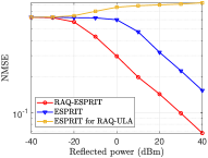
(a)

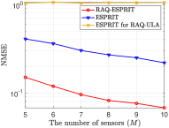
(b)

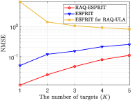
(c)

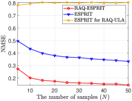
(d)

Figure 2: The NMSE vs. (a) the reflected power of $s_{k}$, (b) the number of sensors ($M$), (c) the number of targets ($K$), and (d) the number of samples ($N$).

IV-B Simulation Results

Upon fixing $M=10$, $K=5$, $N=50$, and varying the power reflected from the targets, we present the simulation results of RAQ-ESPRIT, and of the conventional ESPRIT in Fig. 2(a). We also plot the curve of applying the conventional ESPRIT to the RAQ-ULA for showing its infeasibility. We note that the reflected power affects the received signal-to-noise-ratio (SNR), which is different for the RAQR and for the conventional RF receiver due to the different noise floor experienced and the effective receiver aperture. We observe that the RAQ-ESPRIT exhibits a significant reduction in the NMSE. Specifically, the RAQ-ESPRIT is capable of detecting a $20$ dB weaker signal than the conventional ESPRIT when they have the similar NMSE. This can further facilitate the probability of detection. Then, we determine the number of sensors $M$ by fixing $K=3$, $N=50$, and $20$ dBm reflected power, where the curves are presented in Fig. 2(b). As $M$ increases, both the NMSE curves decrease, but the RAQ-ESPRIT significantly outperforms its conventional counterpart. Furthermore, we present the NMSE vs. the number of targets $K$ in Fig. 2(c) by fixing $M=10$, $N=50$, and $20$ dBm reflected power. As $K$ increases, both curves increase, but RAQ-ESPRIT has a much lower NMSE. Finally, we compare RAQ-ESPRIT to the conventional ESPRIT in terms of the number of samples $N$ in Fig. 2(d) by fixing $M=10$, $K=5$ and $20$ dBm reflected power. We observe that both curves become flat for larger $N$, but the RAQ-ESPRIT more significantly reduces the NMSE than its conventional counterpart.

V Conclusions

In this article, we have conceived RAQRs for the classic DOA estimation problem. To this end, we have designed a RAQ-ULA architecture for detecting multiple targets and constructed its equivalent baseband signal model. Our signal model is in line with the actual implementation of a RAQR, paving the way for future RAQR aided wireless sensing designs. Based on our model, we have also proposed a RAQ-ESPRIT method for DOA estimation with the aid of a RAQ-ULA. Lastly, we have performed simulations for demonstrating the superiority of our scheme.

References

- [1] N. Schlossberger, N. Prajapati, S. Berweger, A. P. Rotunno, A. B. Artusio-Glimpse, M. T. Simons, A. A. Sheikh, E. B. Norrgard, S. P. Eckel, and C. L. Holloway, “Rydberg states of alkali atoms in atomic vapour as SI-traceable field probes and communications receivers,” Nat. Rev. Phys., pp. 1–15, 2024.
- [2] H. Zhang, Y. Ma, K. Liao, W. Yang, Z. Liu, D. Ding, H. Yan, W. Li, and L. Zhang, “Rydberg atom electric field sensing for metrology, communication and hybrid quantum systems,” Sci. Bull., vol. 69, no. 10, pp. 1515–1535, 2024.
- [3] T. Gong, A. Chandra, C. Yuen, Y. L. Guan, R. Dumke, C. M. S. See, M. Debbah, and L. Hanzo, “Rydberg atomic quantum receivers for classical wireless communication and sensing,” arXiv preprint arXiv:2409.14501, 2024.
- [4] E. G. Larsson, O. Edfors, F. Tufvesson, and T. L. Marzetta, “Massive MIMO for next generation wireless systems,” IEEE Commun. Mag., vol. 52, no. 2, pp. 186–195, 2014.
- [5] T. Gong, P. Gavriilidis, R. Ji, C. Huang, G. C. Alexandropoulos, L. Wei, Z. Zhang, M. Debbah, H. V. Poor, and C. Yuen, “Holographic MIMO communications: Theoretical foundations, enabling technologies, and future directions,” IEEE Commun. Surveys Tuts., vol. 26, no. 1, pp. 196–257, 2024.
- [6] F. Liu, Y. Cui, C. Masouros, J. Xu, T. X. Han, Y. C. Eldar, and S. Buzzi, “Integrated sensing and communications: Toward dual-functional wireless networks for 6G and beyond,” IEEE J. Sel. Areas Commun., vol. 40, no. 6, pp. 1728–1767, 2022.
- [7] M. Jing, Y. Hu, J. Ma, H. Zhang, L. Zhang, L. Xiao, and S. Jia, “Atomic superheterodyne receiver based on microwave-dressed Rydberg spectroscopy,” Nat. Phys., vol. 16, no. 9, pp. 911–915, Sep. 2020.
- [8] S. Borówka, U. Pylypenko, M. Mazelanik, and M. Parniak, “Continuous wideband microwave-to-optical converter based on room-temperature Rydberg atoms,” Nat. Photon., vol. 18, no. 1, pp. 32–38, 2024.
- [9] H. Huang, J. Yang, H. Huang, Y. Song, and G. Gui, “Deep learning for super-resolution channel estimation and DOA estimation based massive MIMO system,” IEEE Trans. Veh. Technol., vol. 67, no. 9, pp. 8549–8560, 2018.
- [10] A. H. Shaikh, X. Dang, and D. Huang, “DOA estimation using antenna arrays: A universal array designing framework,” IEEE Trans. Veh. Technol., vol. 72, no. 11, pp. 15 092–15 097, 2023.
- [11] A. K. Robinson, N. Prajapati, D. Senic, M. T. Simons, and C. L. Holloway, “Determining the angle-of-arrival of a radio-frequency source with a Rydberg atom-based sensor,” Appl. Phys. Lett., vol. 118, no. 11, Mar. 2021.
- [12] R. Mao, Y. Lin, Y. Fu, Y. Ma, and K. Yang, “Digital beamforming and receiving array research based on Rydberg field probes,” IEEE Trans. Antennas Propag., vol. 72, no. 2, pp. 2025–2029, 2024.
- [13] D. Richardson, J. Dee, B. Kayim, B. Sawyer, R. Wyllie, R. Lee, and R. Westafer, “Study of angle of arrival estimation with linear arrays of simulated Rydberg atom receivers,” Authorea Preprints, Oct. 2023.
- [14] M. T. Simons, A. H. Haddab, J. A. Gordon, D. Novotny, and C. L. Holloway, “Embedding a Rydberg atom-based sensor into an antenna for phase and amplitude detection of radio-frequency fields and modulated signals,” IEEE Access, vol. 7, pp. 164 975–164 985, 2019.
- [15] T. Gong, J. Sun, C. Yuen, G. Hu, Y. Zhao, Y. L. Guan, C. M. S. See, M. Debbah, and L. Hanzo, “Rydberg atomic quantum receivers for classical wireless communications and sensing: Their models and performance,” arXiv preprint arXiv:2412.05554, 2024.