A Stable Measure for Conditional Periodicity of Time Series using Persistent Homology

Abstract

Given a pair of time series over the same time period, we study how the periodicity of one influences the periodicity of the other. There are several known methods to measure the similarity between a pair of time series, such as cross-correlation, coherence, cross-recurrence, and dynamic time warping. While there are experimental results to show robustness of these similarity measures, we have yet to find any measures with known theoretical stability results.

Persistence homology has been utilized to construct a scoring function with theoretical guarantees of stability that quantifies the periodicity of a single univariate time series $\displaystyle f_{1}$, denoted $\displaystyle\operatorname{score}(f_{1})$. Building on this concept, we propose a conditional periodicity score that quantifies the periodicity of one univariate time series $\displaystyle f_{1}$ given another $\displaystyle f_{2}$, denoted $\displaystyle\operatorname{score}(f_{1}|f_{2})$, and derive theoretical stability results for the same. Dimension reduction techniques are often used on time series data to reduce computational costs. With this setting in mind, we prove a new stability result for $\displaystyle\operatorname{score}(f_{1}|f_{2})$ under principal component analysis (PCA) when we use the projections of the time series embeddings onto their respective first $\displaystyle K$ principal components. We show that the change in our score is bounded by a function of the eigenvalues corresponding to the remaining (unused) $\displaystyle N-K$ principal components and hence is small when the first $\displaystyle K$ principal components capture most of the variation in the time series embeddings. Finally we derive a lower bound on the minimum embedding dimension to use in our pipeline which guarantees that any two such embeddings give scores that are within $\displaystyle\epsilon$ of each other.

We present a procedure for computing conditional periodicity scores and implement it on several pairs of synthetic signals. We experimentally compare our similarity measure to the most-similar statistical measure of cross-recurrence, and show the increased accuracy and stability of our score when predicting and measuring whether or not the periodicities of two time series are similar.

Keywords: time series, conditional periodicity, persistent homology, PCA.

1 Introduction

A continuous univariate time series $\displaystyle f:T\rightarrow\mathbb{R}$ defined on the real-valued interval $\displaystyle T$ is a collection of points $\displaystyle\{f(t)\}$ that depend on the input measure of time, $\displaystyle t\in T$. Time series analysis is employed in numerous applications and measuring the similarity between pairs of univariate time series is a well-studied problem. Cross-correlation coefficients measure the similarity of two series at a given time lag between them and has been used to measure the intensity of earthquakes and identify common significant periods between nucleic signals [13]. Coherence measures the similarity between the power spectra of two signals at a given frequency, and has been used to estimate the correlation between non-stationary EEG and EMG signals [28], detect short significant coherence between non-stationary neural signals [15], and to estimate the correlation between green investment and environmental sustainability in China [29]. Cross-recurrence measures the similarity between the phase space embeddings of two time series, and has been used to quantify the structure of utterance signals between children and their parents [10] and identify different functional movement levels between patients with and without ACL surgery using EEG and EMG signals [22]. Dynamic time warping (DTW) measures the distance between two discrete time series and has been used to cluster time series and identify similarities. More specifically, DTW has been used for clustering suicidal symptoms signals and identifying common dynamics between suicidal ideation and feelings of entrapment, rumination, and depression [9], identifying similar dynamics between manic and depressive symptoms signals [19], and identifying patterns of motion behavior of marine ships for marine trafficking signals [26].

These measures indirectly quantify the similarity between periodicities of time series via integration, power spectra, phase-space embeddings, and the original series themselves. The more similar the periodicities of two series, the smaller the time lag yielding the maximum cross-correlation is. As well, more-similar periodicities yield higher coherence at the input frequency corresponding to the closest approximation of their true underlying frequency. Furthermore, closer periodicities produce more-correlated phase-space embeddings and hence more regions of cross-recurring states. Lastly, increased similarity between periodicities produce smaller DTW distances.

Many of these measures require a correct choice of input parameter in order to identify the quantification of the similarity between periodicities. For instance, one must choose the correct choice of time lag to detect periodicity similarity via cross-correlation, the correct choice of frequency to detect periodicity similarity via coherence, and a suitable choice of distance threshold to detect similarity in the cross-recurrence matrix. At the same time, we have yet to find results demonstrating the theoretical stability of these similarity measures. Persistent homology, on the other hand, provides a natural framework for the theoretical stability of topological summaries. As such, we use persistent homology to define a new similarity measure between two univariate time series that is guaranteed theoretically to be stable, and is directly comparable to cross-recurrence. More specifically, our similarity measure uses persistent homology to quantify how similar the periodicities of two time series are.

1.1 Our contributions

We define a new measure termed the conditional periodicity score of a time series given another time series with a smaller period (Definition 2.6). Our measure provides a new, more-direct, approach to quantifying periodicity similarity between time series as opposed to other previously used measures such as cross-correlation, cross-recurrence, coherence, and dynamic time warping. The main benefit of our conditional periodicity score as opposed to these measures is its guaranteed theoretical stability under small changes in periodicity (Theorem 3.2). Furthermore, in the context of time series analysis under dimension reduction, we show that our score satisfies a stability result even when one uses truncated versions of the time series embeddings as computed by principal component analysis (PCA) (Theorem 3.3 and Corollary 3.4). Finally, we derive a lower bound on the embedding dimensions used that allows us to control the precision of the conditional periodicity score (Theorem 3.5).

We present an algorithm to quantify the conditional periodicity of two input time series using PCA (Algorithm 1). This algorithm runs in $\displaystyle\mathcal{O}\Big{(}P\log{P}+NK^{2}+N^{6}\Big{)}$ time where $\displaystyle P$ is the number of points in the two discrete univariate input signals, $\displaystyle N$ is the number of points in the conditional sliding window embedding (SWE) of the fitted continuous signals, and $\displaystyle K$ is the number of principal components used ($\displaystyle K\leq M+1$ for embedding dimension $\displaystyle M$). We present computational evidence that shows our scoring function is robust to input signals of different types including sinusoidals, dampened sinusoidals, sawtooth-like series, and square-waves (Figure 1) with moderate amounts of Gaussian noise and dampening. In addition, our conditional periodicity score, when compared to its most-similar measure cross-recurrence, is shown experimentally to be superior and maintain greater stability when predicting and measuring whether or not two series’ periodicities are similar (Figures 2–9).

1.2 Related Work

As previously mentioned, many similarity measures that indirectly quantify the closeness of periodicities have been widely used, but we have yet to find any known theoretical stability results for these. These include cross-correlation, coherence, cross-recurrence, and DTW. Persistent homology, on the other hand, has been utilized to quantify the periodicity of a single univariate time series with theoretically shown stability [20, 21, 24, 25]. Inspired by Takens embedding [23], one selects an embedding dimension $\displaystyle M\in\mathbb{N}$ and a time lag $\displaystyle\tau>0$, and maps each time-series point $\displaystyle f(t)$ from a univariate series to an $\displaystyle(M+1)$-dimensional point via the map

$$\operatorname{SW}_{M,\tau}f(t)=\Big{(}f(t),f(t+\tau),\ldots,f(t+M\tau)\Big{)}^{T}.$$

In other words, one maps windows of size $\displaystyle M\tau$ of the input signal to one vector in a point cloud in $\displaystyle\mathbb{R}^{M+1}$. Further, if the series is periodic on $\displaystyle[0,2\pi]$, the resulting point cloud will be an elliptic curve that is roundest when the sliding window size is proportional to the underlying periodicity of the time series. One then performs Vietoris-Rips (VR) filtration on the sliding windows embedding, $\displaystyle\operatorname{SW}_{M,\tau}f(t)$. The more periodic the input signal is, the more rounded the sliding windows embedding is. This yields a higher lifetime of the longest-surviving hole, called maximum 1D-persistence. Dividing this maximum lifetime by the square root of three (assuming the sliding windows embedding (SWE) is centered and normalized) yields a periodicity score between 0 and 1, denoted $\displaystyle\operatorname{score}(f)$, where $\displaystyle\operatorname{score}(f)$ is closer to 1 when $\displaystyle f$ is more periodic. This periodicity score and its aforementioned properties were introduced by Perea and Harer [20], and further used to quantify the periodicity of gene-expressions data by Perea, Deckard, Haase, and Harer  [21]. The stability of this scoring function is proven by the authors [20] using the well-known stability result for persistent homology [5, 6]:

$$\operatorname{d_{B}}\Big{(}\operatorname{dgm}(\operatorname{VR}(X)),\operatorname{dgm}(\operatorname{VR}(Y))\Big{)}\leq 2\operatorname{d_{GH}}(X,Y)\leq 2\operatorname{d_{H}}(X,Y)$$ (1)

where the finite data sets of points $\displaystyle X$ and $\displaystyle Y$ lay in a common metric space. Here, $\displaystyle\operatorname{dgm}(\operatorname{VR}(X))$ and $\displaystyle\operatorname{dgm}(\operatorname{VR}(Y))$ denote the persistence diagrams obtained from VR filtration on the point clouds $\displaystyle X$ and $\displaystyle Y$, $\displaystyle\operatorname{d_{B}}\Big{(}\operatorname{dgm}(\operatorname{VR}(X)),\operatorname{dgm}(\operatorname{VR}(Y))\Big{)}$ defines the bottleneck distance between persistence diagrams $\displaystyle\operatorname{dgm}(\operatorname{VR}(X))$ and $\displaystyle\operatorname{dgm}(\operatorname{VR}(Y))$, $\displaystyle\operatorname{d_{GH}}(X,Y)$ denotes the Gromov-Hausdorff distance between $\displaystyle X$ and $\displaystyle Y$, and $\displaystyle\operatorname{d_{H}}(X,Y)$ denotes the Hausdorff distance between $\displaystyle X$ and $\displaystyle Y$. Since we use the VR filtration by default in this work, we will write $\displaystyle\operatorname{dgm}(X)$ in short to denote $\displaystyle\operatorname{dgm}(\operatorname{VR}(X))$ when there is no cause for confusion.

2 Definitions

Here we introduce standard definitions of distances used in this paper. See, for instance, the book by Burago, Bugaro, and Ivanov [4] for details.

Definition 2.1 (Hausdorff Distance).

Given two sets of points $\displaystyle X$ and $\displaystyle Y$ in a common metric space, the Hausdorff distance between them is given by
$\displaystyle\operatorname{d_{H}}(X,Y)=\inf{\{\epsilon>0:X\subseteq Y^{\epsilon},Y\subseteq X^{\epsilon}\}}$, where $\displaystyle X^{\epsilon}=\underset{x\in X}{\bigcup}B_{\epsilon}(x)$ and $\displaystyle Y^{\epsilon}=\underset{y\in Y}{\bigcup}B_{\epsilon}(y)$ denote the union of all $\displaystyle\epsilon$-balls centered at each point in either set.

Definition 2.2 (Hausdorff Definition of Gromov-Hausdorff Distance).

Given two sets of points $\displaystyle X$ and $\displaystyle Y$, the Gromov-Hausdorff distance between them is given by
$\displaystyle\operatorname{d_{GH}}(X,Y)=\inf{\{\operatorname{d_{H}}(f(X),g(Y)):f:X\rightarrow S,g:Y\rightarrow S\}}$, where $\displaystyle f$ and $\displaystyle g$ are isometric embeddings of $\displaystyle X$ and $\displaystyle Y$ into a common metric space $\displaystyle S$. If $\displaystyle X$ and $\displaystyle Y$ lay in a shared metric space $\displaystyle S$, than $\displaystyle\operatorname{d_{GH}}(X,Y)\leq\operatorname{d_{H}}(X,Y)$ [1].

Definition 2.3 (Distortion Definition of Gromov-Hausdorff Distance).

An alternative definition of the Gromov-Hausdorff distance between two sets of points $\displaystyle X$ and $\displaystyle Y$ is given by
$\displaystyle\operatorname{d_{GH}}(X,Y)=\frac{1}{2}\inf{\{\operatorname{dis}(R):R:X\rightarrow Y}\in\mathcal{R}(X,Y)\}$, where $\displaystyle R$ is a relation between $\displaystyle X$ and $\displaystyle Y$ whose distortion can be defined by $\displaystyle\operatorname{dis}(R)=\sup\{|d_{X}(x,x^{\prime})-d_{Y}(y,y^{\prime})|\,:\,(x,y),(x^{\prime},y^{\prime})\in R\}$, where $\displaystyle d_{X}$ and $\displaystyle d_{Y}$ are the corresponding metrics for $\displaystyle X$ and $\displaystyle Y$, respectively.

Definition 2.4 (Bottleneck Distance).

Given two finite sets of points $\displaystyle X$ and $\displaystyle Y$, let $\displaystyle\operatorname{dgm}(X)$ and $\displaystyle\operatorname{dgm}(Y)$ denote the persistence diagrams of a chosen dimension obtained from Vietoris-Rips (VR) filtration on $\displaystyle X$ and $\displaystyle Y$, respectively. Then the Bottleneck distance between $\displaystyle\operatorname{dgm}(X)$ and $\displaystyle\operatorname{dgm}(Y)$ is given by $\displaystyle\operatorname{d_{B}}(\operatorname{dgm}(X),\operatorname{dgm}(Y))=\underset{\phi}{\inf}\underset{x}{\sup}||x-\phi(x)||_{\infty}$, where $\displaystyle\phi:\operatorname{dgm}(X)\rightarrow\operatorname{dgm}(Y)$ denotes a bijection between $\displaystyle\operatorname{dgm}(X)$ and $\displaystyle\operatorname{dgm}(Y)$, including points along the diagonal in either diagram when they both do not share the same cardinality.

2.1 The Conditional Periodicity Score

We now present the definitions of our measure for the conditional periodicity of two univariate time series.

Definition 2.5 (Conditional Sliding Windows Embedding).

Let $\displaystyle f_{1},f_{2}:[0,2\pi]\rightarrow\mathbb{R}$ be two continuous, periodic, univariate time series with cycle-lengths $\displaystyle\frac{2\pi}{w_{1}}$ and $\displaystyle\frac{2\pi}{w_{2}}$, respectively. Assume $\displaystyle w_{1},w_{2}\in\mathbb{N}$, and that $\displaystyle\frac{2\pi}{w_{2}}\leq\frac{2\pi}{w_{1}}$. Then the conditional sliding windows embedding (SWE) of $\displaystyle f_{1}$ given $\displaystyle f_{2}$ is defined by

$$\operatorname{SW}_{M,\tau}f_{1|2}(t)=\Big{(}f_{1}(t),f_{1}(t+\tau),\ldots,f_{1}(t+M\tau)\Big{)}^{T}$$

where $\displaystyle M\in\mathbb{N}$ is a selected embedding dimension and the time lag $\displaystyle\tau=\frac{2\pi}{w_{2}(M+1)}$ is proportional to the length of one cycle of $\displaystyle f_{2}$.

Definition 2.6 (Conditional Periodicity Score).

Let $\displaystyle\operatorname{mp}(\operatorname{dgm}_{1}(\operatorname{SW}_{M,\tau}f_{1|2}(T))$ denote the lifetime of the longest surviving one dimensional hole in VR filtration on the conditional SWE of $\displaystyle f_{1}$ given $\displaystyle f_{2}$. Then the conditional periodicity score of $\displaystyle f_{1}$ given $\displaystyle f_{2}$ is given by

$$\operatorname{score}(f_{1}|f_{2})=\frac{\operatorname{mp}(\operatorname{dgm}_{1}(\operatorname{SW}_{M,\tau}f_{1|2}(T)))}{\sqrt{3}}$$

for $\displaystyle T=\left[0,\frac{2\pi}{w_{1}}\right]$.

3 Stability Results for the Conditional Periodicity Score

To obtain $\displaystyle\operatorname{score}(f_{1}|f_{2})$, we first compute the conditional SWE of $\displaystyle f_{1}$ given a more-periodic series $\displaystyle f_{2}$ (Definition 2.5), and then perform VR filtration on this embedding to obtain the conditional periodicity score (Definition 2.6). Assuming that $\displaystyle f_{2}$ is more-periodic than $\displaystyle f_{1}$, we ultimately deduce that small changes in periodicity of $\displaystyle f_{2}$ yield small changes in the conditional periodicity score. We assume that $\displaystyle f_{1}$ and $\displaystyle f_{2}$ are continuous series defined on $\displaystyle[0,2\pi]$ where $\displaystyle f_{2}$ is more periodic than $\displaystyle f_{1}$, i.e., $\displaystyle\frac{2\pi}{w_{2}}\leq\frac{2\pi}{w_{1}}$ for $\displaystyle w_{1},w_{2}\in\mathbb{N}$. We also assume that any conditional SWE contains $\displaystyle N\in\mathbb{N}$ points. We first observe that as the periodicity of $\displaystyle f_{2}$ approaches that of $\displaystyle f_{1}$, the conditional periodicity score reduces to the periodicity score of $\displaystyle f_{1}$.

Proposition 3.1 (Reduction to Periodicity Score).

$$\lim_{\begin{subarray}{c}\frac{2\pi}{w_{2}}\rightarrow\frac{2\pi}{w_{1}}^{-}\end{subarray}}\operatorname{SW}_{M,\tau}f_{1|2}(t)=\operatorname{SW}_{M,\tau}f_{1}(t)\text{ for }t\in\left[0,\frac{2\pi}{w_{1}}\right].$$

Proof.

Let $\displaystyle i\in\{0,1,\ldots,M\}$ for fixed $\displaystyle M\in\mathbb{N}$. Since $\displaystyle f_{1}$ is continuous and differentiable on $\displaystyle[0,2\pi]$ and hence on $\displaystyle(0,2\pi)$, it is continuous and differentiable on any subset $\displaystyle[a,b]\subset[0,2\pi]$ and $\displaystyle(a,b)\subset(0,2\pi)$. Let $\displaystyle t\in[0,2\pi]$. Consider the subinterval $\displaystyle I=\left[t+\frac{2i\pi}{w_{2}(M+1)},t+\frac{2i\pi}{w_{1}(M+1)}\right]$ of $\displaystyle[0,2\pi]$. Then $\displaystyle f_{1}$ is also continuous and differentiable on $\displaystyle I$. By Mean Value Theorem, there exists some $\displaystyle c\in\left(t+\frac{2i\pi}{w_{2}(M+1)},t+\frac{2i\pi}{w_{1}(M+1)}\right)$ such that

$$f^{\prime}_{1}(c)\left[\left(t+\frac{2i\pi}{w_{1}(M+1)}\right)\text{\hskip-2.168pt$\displaystyle-$\hskip-2.168pt}\left(t+\frac{2i\pi}{w_{2}(M+1)}\right)\right]\text{\hskip-2.168pt$\displaystyle=$\hskip 0.0pt}f_{1}\left(t+\frac{2i\pi}{w_{1}(M+1)}\right)-f_{1}\left(t+\frac{2i\pi}{w_{2}(M+1)}\right).$$

Then we get the following equality:

$$\displaystyle\text{\hskip-3.61371pt}\left\lVert\operatorname{SW}_{M,\tau}f_{1|2}(t)-\operatorname{SW}_{M,\tau}f_{1}(t)\right\rVert_{2} \displaystyle=\left(\sum_{i=0}^{M}\left|f_{1}\left(t+\frac{2i\pi}{w_{2}(M+1)}\right)-f_{1}\left(t+\frac{2i\pi}{w_{1}(M+1)}\right)\right|^{2}\right)^{\frac{1}{2}}$$

$$\displaystyle=\left(|f^{\prime}_{1}(c)|^{2}\sum_{i=0}^{M}\left|\left(t+\frac{2i\pi}{w_{2}(M+1)}\right)-\left(t+\frac{2i\pi}{w_{1}(M+1)}\right)\right|^{2}\right)^{\frac{1}{2}}$$

$$\displaystyle=\left(|f^{\prime}_{1}(c)|^{2}\left|\frac{1}{M+1}\right|^{2}\left|\frac{2\pi}{w_{2}}-\frac{2\pi}{w_{1}}\right|^{2}\sum_{i=0}^{M}|i|^{2}\right)^{\frac{1}{2}}$$

$$\displaystyle=\frac{|f^{\prime}_{1}(c)|}{(M+1)}\left\lVert\mathbf{v}\right\rVert_{2}\left|\frac{2\pi}{w_{2}}-\frac{2\pi}{w_{1}}\right|$$

where $\displaystyle\mathbf{v}=(0,1,\ldots,M)^{T}$. Then, since $\displaystyle M$ is fixed, we have that

$$\displaystyle\lim_{\frac{2\pi}{w_{2}}\rightarrow\frac{2\pi}{w_{1}}^{-}}\,\left\lVert\operatorname{SW}_{M,\tau}f_{1|2}(t)-\operatorname{SW}_{M,\tau}f_{1}(t)\right\rVert_{2}=\lim_{\frac{2\pi}{w_{2}}\rightarrow\frac{2\pi}{w_{1}}^{-}}\frac{|f^{\prime}_{1}(c)|}{M+1}||\mathbf{v}||_{2}\left|\frac{2\pi}{w_{2}}-\frac{2\pi}{w_{1}}\right|=0.\hskip 21.68121pt\qed$$

A direct consequence of Proposition 3.1 is that $\displaystyle\operatorname{score}(f_{1}|f_{2})\rightarrow\operatorname{score}(f_{1})$ as $\displaystyle\frac{2\pi}{w_{2}}\rightarrow\frac{2\pi}{w_{1}}^{-}$.

Theorem 3.2 (Stability of Conditional Periodicity Score).

Let $\displaystyle f_{1},f_{21},f_{22}:[0,2\pi]\rightarrow\mathbb{R}$ be three continuous univariate time series such that $\displaystyle\frac{2\pi}{w_{22}}<\frac{2\pi}{w_{21}}\leq\frac{2\pi}{w_{1}}$ and $\displaystyle w_{1},w_{21},w_{22}\in\mathbb{N}$. Define the conditional SWE of $\displaystyle f_{1}$ given $\displaystyle f_{21}$ as $\displaystyle X_{1}$ and the conditional SWE of $\displaystyle f_{1}$ given $\displaystyle f_{22}$ as $\displaystyle X_{2}$, where the sliding window sizes are defined using time lags $\displaystyle\tau_{1}=\frac{2\pi}{w_{21}(M+1)}$ and $\displaystyle\tau_{2}=\frac{2\pi}{w_{22}(M+1)}$, respectively. Similarly, define the 1D persistence diagrams from the VR filtrations on $\displaystyle X_{1}$ and $\displaystyle X_{2}$ as $\displaystyle\operatorname{dgm}_{1}(X_{1})$ and $\displaystyle\operatorname{dgm}_{1}(X_{2})$, respectively. Let the max 1D persistence in each diagram be denoted by $\displaystyle\operatorname{mp}(\operatorname{dgm}_{1}(X_{1}))$ and $\displaystyle\operatorname{mp}(\operatorname{dgm}_{1}(X_{2}))$, and the resulting conditional periodicity scores of $\displaystyle f_{1}$ given $\displaystyle f_{21}$ and $\displaystyle f_{1}$ given $\displaystyle f_{22}$ be denoted by $\displaystyle\operatorname{score}(f_{1}|f_{21})$ and $\displaystyle\operatorname{score}(f_{1}|f_{22})$, respectively. Then the following results hold:

$$\operatorname{d_{H}}(X_{1},X_{2})\leq\sqrt{M+1}\,|f_{1}^{\prime}(c)|\left|\frac{2\pi}{w_{21}}-\frac{2\pi}{w_{22}}\right|$$ (2)

$$\operatorname{d_{B}}(\operatorname{dgm}_{1}(X_{1}),\operatorname{dgm}_{1}(X_{2}))\leq 2\sqrt{M+1}\,|f_{1}^{\prime}(c)|\left|\frac{2\pi}{w_{21}}-\frac{2\pi}{w_{22}}\right|$$ (3)

$$\left|\operatorname{mp}(\operatorname{dgm}_{1}(X_{1}))-\operatorname{mp}(\operatorname{dgm}_{1}(X_{2}))\right|\leq 4\sqrt{M+1}\,|f_{1}^{\prime}(c)|\left|\frac{2\pi}{w_{21}}-\frac{2\pi}{w_{22}}\right|$$ (4)

$$\left|\operatorname{score}(f_{1}|f_{21})-\operatorname{score}(f_{1}|f_{22})\right|\leq 4\sqrt{\frac{M+1}{3}}\,|f_{1}^{\prime}(c)|\left|\frac{2\pi}{w_{21}}-\frac{2\pi}{w_{22}}\right|$$ (5)

for some $\displaystyle c\in(t+i\tau_{2},t+i\tau_{1})$ and $\displaystyle i=1,\ldots,M+1$.

Proof.

Proof of bound on Hausdorff distance in Equation (2):

We first find an upper bound on the Euclidean distance between respective pairs of points in $\displaystyle X_{1}$ and $\displaystyle X_{2}$, and then use it to find an upper bound on the Hausdorff distance between the two point clouds. We first claim that

$$\left\lVert\operatorname{SW}_{M,\tau_{1}}f_{1|21}(t)-\operatorname{SW}_{M,\tau_{2}}f_{1|22}(t)\right\rVert_{2}\leq\sqrt{M+1}\,|f_{1}^{\prime}(c)|\left|\frac{2\pi}{w_{21}}-\frac{2\pi}{w_{22}}\right|.$$

Similar to the proof of Proposition 3.1, there exists some $\displaystyle c\in(t+i\tau_{2},t+i\tau_{1})$ where

$$\left\lVert\operatorname{SW}_{M,\tau}f_{1|21}(t)-\operatorname{SW}_{M,\tau}f_{1|22}(t)\right\rVert_{2}=\frac{|f^{\prime}_{1}(c)|}{M+1}\,\left\lVert\mathbf{v}\right\rVert_{2}\left|\frac{2\pi}{w_{21}}-\frac{2\pi}{w_{22}}\right|\text{ for }\mathbf{v}=(0,1,\ldots,M)^{T}.$$

Then $\displaystyle\left\lVert\mathbf{v}\right\rVert_{2}=\sqrt{\sum_{i=0}^{M+1}|i|^{2}}\leq\sqrt{(M+1)(M+1)^{2}}$ and hence

$$\left\lVert\operatorname{SW}_{M,\tau}f_{1|21}(t)-\operatorname{SW}_{M,\tau}f_{1|22}(t)\right\rVert_{2}\leq\sqrt{M+1}\,|f_{1}^{\prime}(c)|\left|\frac{2\pi}{w_{21}}-\frac{2\pi}{w_{22}}\right|.$$

Let $\displaystyle\epsilon>\sqrt{M+1}\,|f_{1}^{\prime}(c)|\left|\frac{2\pi}{w_{21}}-\frac{2\pi}{w_{22}}\right|$. Then $\displaystyle X_{1}\subset X_{2}^{\epsilon}$ and $\displaystyle X_{2}\subset X_{1}^{\epsilon}$, so by Definition 2.1, $\displaystyle\operatorname{d_{H}}(X_{1},X_{2})\leq\epsilon$. Taking the infimum of both sides yields the relation

$$\operatorname{d_{H}}(X_{1},X_{2})\leq\sqrt{M+1}\,|f_{1}^{\prime}(c)|\left|\frac{2\pi}{w_{21}}-\frac{2\pi}{w_{22}}\right|.$$

Proof of bound on bottleneck distance in Equation (3):

By the bound on stability of persistence diagrams in Equation (1), we have that $\displaystyle\operatorname{d_{B}}(\operatorname{dgm}_{1}(X_{1}),$ $\displaystyle\operatorname{dgm}_{1}(X_{2}))\leq 2\operatorname{d_{H}}(X_{1},X_{2})$, since $\displaystyle X_{1}$ and $\displaystyle X_{2}$ both lay in $\displaystyle\mathbb{R}^{M+1}$.

Proof of bound on max persistence in Equation (4):

Let $\displaystyle(b_{1}^{\max},d_{1}^{\max})$ and $\displaystyle(b_{2}^{\max},d_{2}^{\max})$ be the points corresponding to the 1D-features of max persistence in $\displaystyle\operatorname{dgm}_{1}(X_{1})$ and $\displaystyle\operatorname{dgm}_{1}(X_{2})$. Let $\displaystyle\epsilon^{\ast}=\operatorname{d_{B}}(\operatorname{dgm}_{1}(X_{1}),\operatorname{dgm}_{1}(X_{2}))$. Then by Definition 2.4, any pairs of points $\displaystyle(b_{1},d_{1})$ and $\displaystyle(b_{2},d_{2})$ in the respective diagrams satisfy $\displaystyle||(b_{1},d_{1})-(b_{2},d_{2})||_{\infty}=\sup{\{|b_{1}-b_{2}|,|d_{1}-d_{2}|\}}\leq\epsilon^{\ast}$. Hence, $\displaystyle|b_{1}^{\max}-b_{2}^{\max}|\leq\epsilon^{\ast}$ and $\displaystyle|d_{1}^{\max}-d_{2}^{\max}|\leq\epsilon^{\ast}$. Therefore

$$|\operatorname{mp}(\operatorname{dgm}_{1}(X_{1}))-\operatorname{mp}(\operatorname{dgm}_{1}(X_{2}))|\leq|d_{1}^{\max}-d_{2}^{\max}|+|b_{1}^{\max}-b_{2}^{\max}|\leq 2\operatorname{d_{B}}(\operatorname{dgm}_{1}(X_{1}),\operatorname{dgm}_{1}(X_{2})).$$

Proof of bound on score in Equation (5): By Definition 2.6,

$$\displaystyle|\operatorname{score}(f_{1}|f_{21})-\operatorname{score}(f_{1}|f_{22})| \displaystyle=\frac{1}{\sqrt{3}}\left|\operatorname{mp}(\operatorname{dgm}_{1}(X_{1}))-\operatorname{mp}(\operatorname{dgm}_{1}(X_{2}))\right|$$

$$\displaystyle\leq\frac{2}{\sqrt{3}}\operatorname{d_{B}}(\operatorname{dgm}_{1}(X_{1}),\operatorname{dgm}_{1}(X_{2}))$$

$$\displaystyle\leq\frac{4}{\sqrt{3}}\operatorname{d_{H}}(X_{1},X_{2})$$

$$\displaystyle\leq 4\sqrt{\frac{M+1}{3}}\,|f_{1}^{\prime}(c)|\left|\frac{2\pi}{w_{21}}-\frac{2\pi}{w_{22}}\right|.\qed$$

3.1 Stability of Score under PCA

The main bottleneck in using the periodicity score in practice is the computation of the dimension 1 persistence diagram of the Vietoris-Rips filtration of the SWE. In general, for a point cloud $\displaystyle X$ with $\displaystyle N$ points, the computation of $\displaystyle\operatorname{dgm}_{1}(X)$ runs in $\displaystyle O(N^{6})$ time, although faster approaches may be available in lower dimensions [14, 30]. Hence, we study the conditional periodicity score under principal component analysis (PCA), a widely used dimension reduction technique [12].

Theorem 3.3 (Stability of Conditional Periodicity Score Under PCA).

Let $\displaystyle K\leq M+1$ for $\displaystyle K\in\mathbb{N}$. Suppose $\displaystyle f_{2}$ is more periodic than $\displaystyle f_{1}$ on $\displaystyle[0,2\pi]$ with cycle lengths $\displaystyle\frac{2\pi}{w_{2}}\leq\frac{2\pi}{w_{1}}$, respectively. For $\displaystyle T=\left[0,\frac{2\pi}{w_{1}}\right]$, define the orthogonal projection of $\displaystyle X=\operatorname{SW}_{M,\tau}f_{1|2}(T)$ onto its top $\displaystyle K$ principal components by $\displaystyle\phi(X)=(\langle\mathbf{c}_{1},X\rangle,\ldots,\langle\mathbf{c}_{K},X\rangle)^{T}$ for orthonormal eigenvectors and corresponding eigenvalues $\displaystyle\{\mathbf{c}_{k},\lambda_{k}\}_{k=1}^{N}$ produced by PCA. Suppose $\displaystyle X$ contains $\displaystyle N\in\mathbb{N}$ points. Denote the conditional periodicity score under $\displaystyle\phi$ by $\displaystyle\operatorname{score}_{\phi}(f_{1}|f_{2})$. Then

$$|\operatorname{score}(f_{1}|f_{2})-\operatorname{score}_{\phi}(f_{1}|f_{2})|\leq\sqrt{\frac{8}{3}}\sqrt[4]{\sum_{i=K+1}^{N}\lambda_{i}^{2}}.$$

Proof.

Notice that $\displaystyle\phi$ is a relation in $\displaystyle\mathcal{R}(X,Y)$ for $\displaystyle Y=\phi(X)$. Then by Definition 2.3 we have that $\displaystyle\operatorname{d_{GH}}(X,Y)\leq\frac{1}{2}\operatorname{dis}(\phi)$, where $\displaystyle\operatorname{dis}(\phi)^{2}=\left\lVert D_{X}-D_{Y}\right\rVert_{\max}^{2}$ with $\displaystyle D_{X}$ being the matrix of pairwise distances in $\displaystyle X$. We get that [18, Lemma 3.9]

$$\left\lVert D_{X}-D_{Y}\right\rVert_{\max}^{2}\leq\left\lVert D_{X}^{\circ^{2}}-D_{Y}^{\circ^{2}}\right\rVert_{\max},$$

where $\displaystyle D_{X}^{\circ^{2}}$ denotes the matrix of squared pairwise Euclidean distances in $\displaystyle X$.

Recall that for a matrix $\displaystyle A$, $\displaystyle\left\lVert A\right\rVert_{\max}^{2}=\left(\max{{}_{ij}|A_{ij}|}\right)^{2}=\max{{}_{ij}|A_{ij}|^{2}}\leq\sum_{ij}|A_{ij}|^{2}=\left\lVert A\right\rVert_{F}^{2}$, where $\displaystyle\left\lVert\cdot\right\rVert_{F}$ denotes the Frobenius norm. Then we have

$$\left\lVert D_{X}^{\circ^{2}}-D_{Y}^{\circ^{2}}\right\rVert_{\max}\leq\left\lVert D_{X}^{\circ^{2}}-D_{Y}^{\circ^{2}}\right\rVert_{F}.$$

Define the eigendecomposition of the covariance of $\displaystyle X$ as $\displaystyle XX^{T}=Q\Lambda Q^{T}$, where $\displaystyle Q=[\mathbf{c}_{1},\dots,\mathbf{c}_{N}]$ is the $\displaystyle N\times N$ matrix of orthonormal eigenvectors and $\displaystyle\Lambda=\operatorname{diag}(\lambda_{1},\dots,\lambda_{N})$ is the $\displaystyle N\times N$ diagonal matrix of eigenvalues corresponding to the orthogonal projection of $\displaystyle X$. Then the eigendecomposition of the $\displaystyle K$-dimensional subspace containing the top $\displaystyle K$ principal components of $\displaystyle X$ can be defined by $\displaystyle YY^{T}=Q\Lambda|_{K}Q^{T}$, where $\displaystyle\Lambda|_{K}=\operatorname{diag}(\lambda_{1},\dots,\lambda_{K},\underbrace{0,\dots,0}_{N-K})$. Then, if we center the squared distances in $\displaystyle D_{X}^{\circ^{2}}$ and $\displaystyle D_{Y}^{\circ^{2}}$, we obtain the relations [2]

$$\displaystyle XX^{T}=-\frac{1}{2}C_{N}D_{X}^{\circ^{2}}C_{N}$$ and

$$\displaystyle YY^{T}=-\frac{1}{2}C_{N}D_{Y}^{\circ^{2}}C_{N},$$

where $\displaystyle C_{N}$ is the $\displaystyle N\times N$ centering matrix with diagonal entries $\displaystyle 1-\frac{1}{N}$ and off-diagonal entries $\displaystyle-\frac{1}{N}$. Then $\displaystyle D_{X}^{\circ^{2}}=-2C_{N}(Q\Lambda Q^{T})C_{N}$ and $\displaystyle D_{Y}^{\circ^{2}}=-2C_{N}(Q\Lambda|_{K}Q^{T})C_{N}$. Since $\displaystyle Q^{T}Q=QQ^{T}=I$, we obtain that

$$\displaystyle\left\lVert D_{X}^{\circ^{2}}-D_{Y}^{\circ^{2}}\right\rVert_{F} \displaystyle=2\left\lVert C_{N}(Q\Lambda Q^{T}-Q\Lambda|_{K}Q^{T})C_{N}\right\rVert_{F}$$

$$\displaystyle=2\left\lVert Q(\Lambda-\Lambda|_{K})Q^{T}\right\rVert_{F}\quad\text{ since }C_{N}\approx I\text{ for sufficiently large }N$$

$$\displaystyle=2\sqrt{\operatorname{tr}(Q(\Lambda-\Lambda|_{K})^{2}Q^{T})}$$

$$\displaystyle=2\sqrt{\operatorname{tr}((\Lambda-\Lambda|_{K})^{2})}\quad\text{ since trace is cyclically invariant}$$

$$\displaystyle=2\sqrt{\sum_{i=K+1}^{N}\lambda_{i}^{2}}.$$

Thus we get that $\displaystyle\operatorname{dis}(\phi)\leq\sqrt{2}\sqrt[4]{\sum_{i=K+1}^{N}\lambda_{i}^{2}}$ and hence $\displaystyle\operatorname{d_{GH}}(X,Y)\leq\frac{\sqrt{2}}{2}\sqrt[4]{\sum_{i=K+1}^{N}\lambda_{i}^{2}}$. Then again by the standard result on stability of persistence diagrams (Equation (1)), we get that

$$\operatorname{d_{B}}(\operatorname{dgm}_{1}(X),\operatorname{dgm}_{1}(Y))\leq 2\operatorname{d_{GH}}(X,Y)\leq\sqrt{2}\sqrt[4]{\sum_{i=K+1}^{N}\lambda_{i}^{2}}.$$

Hence by similar arguments to those in the proof of Theorem 3.2, we have that

$$\displaystyle|\operatorname{score}(f_{1}|f_{2})-\operatorname{score}_{\phi}(f_{1}|f_{2})| \displaystyle=\frac{1}{\sqrt{3}}\left|\operatorname{mp}(\operatorname{dgm}_{1}(X))-\operatorname{mp}(\operatorname{dgm}_{1}(\phi(X)))\right|$$

$$\displaystyle\leq\frac{2}{\sqrt{3}}\operatorname{d_{B}}(\operatorname{dgm}_{1}(X),\operatorname{dgm}_{1}(\phi(X)))$$

$$\displaystyle\leq 2\sqrt{\frac{2}{3}}\sqrt[4]{\sum_{i=K+1}^{N}\lambda_{i}^{2}}.$$

$$\displaystyle=\sqrt{\frac{8}{3}}\sqrt[4]{\sum_{i=K+1}^{N}\lambda_{i}^{2}}.\qed$$

Theorem 3.3 shows that if the top $\displaystyle K$ principal components of the conditional SWE capture most of its structure, then the conditional periodicity score won’t change much under the associated orthogonal projection. We now reveal a direct consequence of this stability under small changes in periodicity of $\displaystyle f_{2}$.

Corollary 3.4 (Consequence of Stability of Conditional Periodicity Score Under PCA).

Let $\displaystyle K\leq M+1$ for $\displaystyle K\in\mathbb{N}$. Define the orthogonal projection of $\displaystyle X_{1}$ and $\displaystyle X_{2}$ as defined in Theorem 3.2 onto their top $\displaystyle K$ principal components by the relation $\displaystyle\phi(X_{1})=(\langle\mathbf{c}_{1},X_{1}\rangle,\ldots,\langle\mathbf{c}_{K},X_{1}\rangle)^{T}$ and $\displaystyle\phi(X_{2})=(\langle\mathbf{d}_{1},X_{2}\rangle,\ldots,\langle\mathbf{d}_{K},X_{2}\rangle)^{T}$ for orthonormal eigenvectors and corresponding eigenvalues $\displaystyle\{\mathbf{c}_{k},\lambda_{k}\}_{k=1}^{N},\{\mathbf{d}_{k},\gamma_{k}\}_{k=1}^{N}$ produced by PCA. Suppose $\displaystyle X_{1}$ and $\displaystyle X_{2}$ each contain $\displaystyle N\in\mathbb{N}$ points. Define the conditional periodicity score of $\displaystyle f_{1}$ given $\displaystyle f_{21}$ and $\displaystyle f_{1}$ given $\displaystyle f_{22}$ under $\displaystyle\phi$ as $\displaystyle\operatorname{score}_{\phi}(f_{1}|f_{21})$ and $\displaystyle\operatorname{score}_{\phi}(f_{1}|f_{22})$. Then the following inequality holds:

$$\displaystyle\left|\operatorname{score}_{\phi}(f_{1}|f_{21})-\operatorname{score}_{\phi}(f_{1}|f_{22})\right|\leq\sqrt{\frac{8}{3}}\left(\sqrt[4]{\sum_{i=K+1}^{N}\lambda_{i}^{2}}+\sqrt[4]{\sum_{i=K+1}^{N}\gamma_{i}^{2}}\right)$$

$$\displaystyle+~|\operatorname{score}(f_{1}|f_{21})-\operatorname{score}(f_{1}|f_{22})|.$$

Proof.

By Theorem 3.3, we have that

$$|\operatorname{score}_{\phi}(f_{1}|f_{21})-\operatorname{score}(f_{1}|f_{21})|\leq\sqrt{\frac{8}{3}}\sqrt[4]{\sum_{i=K+1}^{N}\lambda_{i}^{2}}\quad\text{and}$$

$$|\operatorname{score}_{\phi}(f_{1}|f_{22})-\operatorname{score}(f_{1}|f_{22})|\leq\sqrt{\frac{8}{3}}\sqrt[4]{\sum_{i=K+1}^{N}\gamma_{i}^{2}}.$$

Hence we get

$$\displaystyle\left|\operatorname{score}_{\phi}(f_{1}|f_{21})-\operatorname{score}_{\phi}(f_{1}|f_{22})\right|\hskip 252.94499pt$$

$$\displaystyle\hskip 36.135pt\leq\left|\operatorname{score}_{\phi}(f_{1}|f_{21})-\operatorname{score}(f_{1}|f_{21})\right|+\left|\operatorname{score}(f_{1}|f_{21})-\operatorname{score}(f_{1}|f_{22})\right|$$

$$\displaystyle\hskip 180.67499pt+\left|\operatorname{score}(f_{1}|f_{22})-\operatorname{score}_{\phi}(f_{1}|f_{22})\right|$$

$$\displaystyle\hskip 36.135pt\leq\sqrt{\frac{8}{3}}\left(\sqrt[4]{\sum_{i=K+1}^{N}\lambda_{i}^{2}}+\sqrt[4]{\sum_{i=K+1}^{N}\gamma_{i}^{2}}\right)+|\operatorname{score}(f_{1}|f_{21})-\operatorname{score}(f_{1}|f_{22})|.$$

∎

Corollary 3.4 reveals that small changes in periodicity of $\displaystyle f_{2}$ still yield small changes in the $\displaystyle\operatorname{score}(f_{1}|f_{2})$ under orthogonal projection if the top $\displaystyle K$ principal components of the conditional SWE capture most of its structure.

3.2 A Minimum Embedding Dimension for Convergence

We define a minimum embedding dimension $\displaystyle\mathcal{M}$ that we can use to control the convergence behavior of the conditional periodicity score $\displaystyle\rm{score}(f_{1}|f_{2})$ near the periodicity score $\displaystyle\rm{score}(f_{1})$.

Theorem 3.5 (Minimum embedding dimension for convergence).

Let $\displaystyle\epsilon>0$. Any embedding dimension $\displaystyle M_{2}>M_{1}\geq\mathcal{M}$ $\displaystyle\in$ $\displaystyle\mathbb{N}$ for $\displaystyle\mathcal{M}=\left\lceil{\frac{2\pi}{w_{2}\epsilon}}\right\rceil$ guarantees that the respective conditional periodicity scores $\displaystyle\rm{score}_{M_{2}}(f_{1}|f_{2})$ and $\displaystyle\rm{score}_{M_{1}}(f_{1}|f_{2})$ are within $\displaystyle\epsilon$ of each other.

Proof.

The conditional periodicity score is determined by $\displaystyle\operatorname{SW}_{M,\tau}f_{1|2}(T)$, $\displaystyle T=\left[0,\frac{2\pi}{w_{1}}\right]$, which is further determined by the width of the sliding window $\displaystyle M\tau$, which for fixed $\displaystyle M$ is determined by the time lag $\displaystyle\tau$. Thus, it suffices to show that $\displaystyle\tau=\frac{2\pi}{w_{2}(M+1)}$ is a Cauchy sequence of $\displaystyle M$. By the definition of $\displaystyle\mathcal{M}$, $\displaystyle\mathcal{M}\geq\frac{2\pi}{w_{2}\epsilon}$ and hence $\displaystyle\frac{2\pi}{w_{2}\mathcal{M}}\leq\epsilon$ $\displaystyle\implies$ $\displaystyle\frac{2\pi}{w_{2}}\left(\frac{1}{\mathcal{M}}\right)\leq\epsilon$. Since $\displaystyle M_{2}>M_{1}\geq\mathcal{M}$, $\displaystyle M_{2}+1>M_{1}+1\geq\mathcal{M}+1$ and hence $\displaystyle\frac{1}{M_{2}+1}<\frac{1}{M_{1}+1}\leq\frac{1}{\mathcal{M}+1}<\frac{1}{\mathcal{M}}$. Thus we get

$$\displaystyle|\tau(M_{1})-\tau(M_{2})| \displaystyle=\frac{2\pi}{w_{2}}\left|\frac{1}{M_{1}+1}-\frac{1}{M_{2}+1}\right|$$

$$\displaystyle=\frac{2\pi}{w_{2}}\left(\frac{1}{M_{1}+1}-\frac{1}{M_{2}+1}\right)$$

$$\displaystyle\leq\frac{2\pi}{w_{2}}\left(\frac{1}{\mathcal{M}+1}-\frac{1}{M_{2}+1}\right)$$

$$\displaystyle<\frac{2\pi}{w_{2}}\left(\frac{1}{\mathcal{M}}\right)\leq\epsilon.\qed$$

Theorem 3.5 tells us that the conditional periodicity score is a Cauchy sequence of the embedding dimension, where smaller values of an $\displaystyle\epsilon$ that we choose yield larger input embedding dimensions that increase the precision of convergence of $\displaystyle\rm{score}(f_{1}|f_{2})$ to $\displaystyle\rm{score}(f_{1})$. This result can be useful if we want to ensure that the conditional scores we are computing are converging to the original periodicity score, albeit at the cost of higher run times due to a larger embedding dimension.

4 Computational Results

We present a framework for computing the conditional periodicity score using PCA. We then apply this framework on periodic signals of multiple types. We also compare the performance of our conditional periodicity score with that of cross-recurrence.

4.1 Procedure for Quantifying Conditional Periodicity

We introduce a procedure for computing the conditional periodicity score of a discrete time series $\displaystyle\{f_{i}(t_{p})\}_{p=1}^{P}$ given another $\displaystyle\{f_{j}(t_{p})\}_{p=1}^{P}$, $\displaystyle P\in\mathbb{N}$ (see Algorithm 1). We first fit two continuous time series $\displaystyle f_{i}^{\text{cts}}$ and $\displaystyle f_{j}^{\text{cts}}$ onto each discrete signal over the interval $\displaystyle[0,2\pi]$ via cubic spline interpolation. We then estimate the length of one cycle of $\displaystyle f_{i}$ and $\displaystyle f_{j}$ using the discrete fast Fourier transform (FFT) on the continuously-fitted series. We assign $\displaystyle f_{1}$ as the series with the larger cycle-length and $\displaystyle f_{2}$ as that with the smaller length. We then compute the top $\displaystyle K$ principal components of the conditional SWE. Assuming the embedding dimension $\displaystyle M+1$ is at least 3, we typically choose $\displaystyle K=2$. We finally perform VR filtration on the SWE, obtaining the conditional periodicity score termed $\displaystyle\operatorname{score}_{\phi}(\cdot)$ under the PCA projection $\displaystyle\phi$.

1

Inputs : Embedding dimension $\displaystyle M\in\mathbb{N}$, $\displaystyle N\in\mathbb{N}$ points in the conditional SWE, and two discrete univariate time series $\displaystyle f_{i},f_{j}$ defined on $\displaystyle\{t_{1},\ldots,t_{P}:P\in\mathbb{N}\}$.

2

3Fit a continuous signal $\displaystyle f_{k}^{\text{cts}}:[0,2\pi]\rightarrow\mathbb{R}$ to the discrete signal $\displaystyle f_{k}$ via cubic spline interpolation such that $\displaystyle f_{k}^{\text{cts}}(0)=f_{k}(t_{1})$ and $\displaystyle f_{k}^{\text{cts}}(2\pi)=f_{k}(t_{P})$ for $\displaystyle k=i,j$.

4Estimate $\displaystyle\frac{2\pi}{w_{i}}$ and $\displaystyle\frac{2\pi}{w_{j}}$ via spectral analysis using the (Discrete) Fast Fourier Transform. Assign $\displaystyle f_{1}$ to be the less periodic and $\displaystyle f_{2}$ to be the more periodic signal of the pair $\displaystyle\left\{f_{i}^{\text{cts}},f_{j}^{\text{cts}}\right\}$. That is, define :

$$\displaystyle\frac{2\pi}{w_{1}}=\max{\left\{\frac{2\pi}{w_{i}},\frac{2\pi}{w_{j}}\right\}},\quad\frac{2\pi}{w_{2}}=\min{\left\{\frac{2\pi}{w_{i}},\frac{2\pi}{w_{j}}\right\}}\quad\quad$$

$$\displaystyle f_{1}=\left\{f_{k}^{\text{cts}}:\frac{2\pi}{w_{k}}=\frac{2\pi}{w_{1}}\right\},\quad f_{2}=\left\{f_{k}^{\text{cts}}:\frac{2\pi}{w_{k}}=\frac{2\pi}{w_{2}}\right\}$$

5Define $\displaystyle\tau=\frac{2\pi}{w_{2}(M+1)}$.

6Compute $\displaystyle X=\operatorname{SW}_{M,\tau}f_{1|2}(T)$ for $\displaystyle N$ evenly-spaced time points in $\displaystyle T=\left[0,\frac{2\pi}{w_{1}}\right]$.

7    For $\displaystyle K=\min\{2,M+1\}$, compute $\displaystyle\phi:\mathbb{R}^{M+1}\rightarrow\mathbb{R}^{K}$, the orthogonal

8     projection of $\displaystyle X$ onto its first $\displaystyle K$ principal components ($\displaystyle K=2$, typically).

9

10Center and normalize $\displaystyle\phi(X)$ to obtain $\displaystyle Y$.

11

12Compute $\displaystyle\operatorname{dgm}_{1}(Y)$ from VR filtration on $\displaystyle Y$ and $\displaystyle\operatorname{mp}(\operatorname{dgm}_{1}(Y))$ from $\displaystyle\operatorname{dgm}_{1}(Y)$.

13Compute $\displaystyle\operatorname{score}_{\phi}(f_{1}|f_{2})$ using $\displaystyle\operatorname{mp}(\operatorname{dgm}_{1}(Y))$.

Return : $\displaystyle\left\{\operatorname{score}_{\phi}(f_{1}|f_{2}),w_{1},w_{2},f_{i}\text{ assignment},f_{j}\text{ assignment}\right\}$.

Algorithm 1 Procedure for quantifying conditional periodicity

Remark 4.1 (Computational Complexity of Conditional Periodicity Score).

Algorithm 1 runs in $\displaystyle O\Big{(}P\log{P}+NK^{2}+N^{6}\Big{)}$ time, where $\displaystyle P$ is the number of points in the discrete univariate input signals $\displaystyle f_{i}$ and $\displaystyle f_{j}$, $\displaystyle N$ is the number of points in the conditional SWE of the fitted continuous signals $\displaystyle f_{1}$ given $\displaystyle f_{2}$, and $\displaystyle K<M+1$ is the number of principal components used for the conditional SWE where $\displaystyle M$ is the embedding dimension. We take $\displaystyle K=2$ by default. The cubic spline interpolation on $\displaystyle f_{i}$ and $\displaystyle f_{j}$ runs in $\displaystyle O(P)$ time [11] and the discrete FFT on $\displaystyle f_{i}^{\text{cts}},f_{j}^{\text{cts}}$ can be computed in $\displaystyle O(P\log P)$ time [3]. The PCA computations run in $\displaystyle O(NK^{2})$ time [12, 27]. The bottleneck step is usually the computation of the 1D persistence diagram using the VR filtration of $\displaystyle Y$, which runs in $\displaystyle O(N^{6})$ time [14, 30].

4.2 Conditional Periodicity Score of Periodic Signals

We demonstrate the stability of the conditional periodicity score on multiple types of periodic signals using Algorithm 1, with added levels of Gaussian noise.

We consider periodic cosine, dampened cosine, sawtooth, and square wave signals with varying levels of dampening (between 5% to 80%) and Gaussian noise (between 0% and 75%) applied to $\displaystyle f_{1}$ and $\displaystyle f_{2}$. We plot one example of graphs for each of these cases in Figure 1. The first column of graphs shows a plot of $\displaystyle f_{1}$ and $\displaystyle f_{2}$ for $\displaystyle w_{1}=3$ and $\displaystyle w_{2}=7$. The second column of graph shows a plot of $\displaystyle\operatorname{score}(f_{1}|f_{2})$ versus $\displaystyle M$ for $\displaystyle M=\{2,\ldots,200\}$. We add a vertical red dashed line to these graphs at embedding dimension $\displaystyle\mathcal{M}=\left\lceil\frac{2\pi}{w_{2}\epsilon}\right\rceil=90$ for $\displaystyle\epsilon=0.01$ and our selected value of $\displaystyle w_{2}$. The third column of graphs shows a plot of $\displaystyle\operatorname{score}(f_{1}|f_{2})$ versus $\displaystyle\frac{2\pi}{w_{2}}$ for $\displaystyle w_{2}=\{w_{1},\ldots,15\}$ and for fixed embedding dimension $\displaystyle\mathcal{M}$.

From top to bottom, the rows in Figure 1 show an example of plots for cosine, dampened, sawtooth, and square wave signals, respectively. For these examples, we fix Gaussian noise to 5% and dampening to 5%. We further define the SMA window widths for these series to be 19, 16, 13, and 13, respectively. Overall, these signals showed stability for up to 75%, 60%, 50%, and 75% noise, respectively, while dampened signals showed stability for up to 40% dampening.

To handle noise, we compute a simple moving average of each signal followed by a mean shift of the conditional SWE. See Section 4.3 for a more in-depth explanation of these denoising techniques, as well as how we selected the simple moving average window width. We fix $\displaystyle P=200$ discrete time points and $\displaystyle N=100$ conditional SWE points in each case.

Figure 1: Conditional periodicity scores of various periodic signal types with added Gaussian noise and dampening. From top to bottom, we show cosine, dampened (5%), sawtooth, and square wave signals results for 5% noise, respectively.

Our results show that our conditional periodicity score is not only stable, but is also robust to different signal types. Our scoring function is more sensitive to signals with sharp discontinuities (i.e. sawtooths and square waves); however, despite this, its convergence still remains stable as the periodicities become closer. Our algorithm also shows consistency of a minimum embedding dimension that controls the convergence of the conditional periodicity score across different signal types with the same periodicity.

4.3 Comparing Conditional Periodicity Score and Cross-Recurrence

Recall that cross-recurrence is a binary measure that examines whether or not the $\displaystyle i$-th point in the SWE of $\displaystyle f_{1}$ is close to the $\displaystyle j$-th point in the SWE of $\displaystyle f_{2}$, where closeness is determined by standard Euclidean distance. Summing up all of the non-noisy cases in which pairs of points from both embeddings are sufficiently close, we get a measure of similarity for cross-recurrence, which is commonly known as the percent determinism, denoted %DET. More specifically, percent determinism is the proportion of cross-recurring states between both phase-space embeddings that are apart of a diagonal strip in the cross-recurrence matrix $\displaystyle C$, and essentially measures how correlated both phase-space embeddings are. Here, less correlation is indicated by lower determinism [16]. We compare our conditional periodicity score to this measure, as both quantifications use the SWEs of $\displaystyle f_{1}$ and $\displaystyle f_{2}$ for measuring how similar their periodicities are.

To handle noise when computing the cross-recurrence matrix, we fix the distance threshold to be greater than five times the standard deviation of Gaussian noise in each case of $\displaystyle f_{2}$ [16]. To handle noise when computing the conditional periodicity score, we perform two denoising methods on the discrete time series and on the resulting conditional SWE. To denoise the input series, we locally average every point in $\displaystyle f_{1}$ and $\displaystyle f_{2}$ by taking the mean of a window of points around it, and repeat this for each point. This process is called a simple moving average and results in two averaged discrete signals. To denoise the conditional SWE of $\displaystyle f_{1}$ given $\displaystyle f_{2}$, we apply a similar process called mean shifting. That is, for each point $\displaystyle\mathbf{v}_{i}$ in the point cloud, we average it with all its neighbors $\displaystyle\mathbf{v}_{j}$, where the angle between $\displaystyle\mathbf{v}_{i}$ and $\displaystyle\mathbf{v}_{j}$ is less than $\displaystyle\frac{\pi}{16}$ [8, 21].

We fix the input parameters for both similarity measures by setting the number of points in each SWE to $\displaystyle N=100$, the number of points in each input series to $\displaystyle P=200$, $\displaystyle w_{1}=3$, and $\displaystyle w_{2}=\{w_{1},\ldots,20\}$. We then fix the tolerance threshold $\displaystyle\text{tol}=5\sigma+2.5$ to determine whether or not the $\displaystyle i$-th and $\displaystyle j$-th points from both embeddings cross-recur, where $\displaystyle\sigma$ is the standard deviation of added Gaussian noise to both signals. This tolerance threshold ultimately determines the %DET values. As well, we fix the precision $\displaystyle\epsilon=0.0005$ to determine the embedding dimension $\displaystyle\mathcal{M}$ in each case of $\displaystyle w_{2}$ (Theorem 3.5). Similarly, this embedding dimension ultimately determines the shape of the SWEs and hence the conditional periodicity score. We select a simple moving average window width of 19 so that it is less than one-third the size of one cycle of $\displaystyle f_{1}$, i.e., $\displaystyle<22$. In this way, we maintain a balance of enough points for denoising while also maintaining the periodic structure of the signals. We construct plots for a range of window widths between 18 and 22 and select the graph showing the most stability of $\displaystyle\operatorname{score}(f_{1}|f_{2})$. We select two as the minimum number of ones determining a diagonal line in $\displaystyle C$, since increasing this minimum decreased the stability of %DET and we want to ensure a fair stability comparison.

We increase the Gaussian noise of both $\displaystyle f_{1}$ and $\displaystyle f_{2}$ from 0% to 12% in increments of 2%, and for each noise level, we obtain a collection of similarity measures for each $\displaystyle w_{2}$. From each collection, we select a percentile from the list $\displaystyle\{15,25,35,45,55,65,75,85\}$ and use it to define a binary cutoff for both meausures. We then collect predicted periodicity-similarities for each noise level and cutoff value as follows. For each pair of cutoffs (one for each measure), if the conditional periodicity score and the percent determinism are greater than or equal to their respective cutoffs, we consider $\displaystyle f_{1}$ and $\displaystyle f_{2}$ to have similar periodicities at the current value of $\displaystyle w_{2}$ and hence store a predicted binary response of one for each measure. Otherwise, we store the predicted similarity as zero for both measures. We then compute the true predicted periodicity-similarities using the same percentile to define the cutoff for $\displaystyle\left|\frac{2\pi}{w_{1}}-\frac{2\pi}{w_{2}}\right|$. Here, any $\displaystyle w_{2}$ producing a distance at most the value of this cutoff yields a true response of one and zero otherwise.

Once we obtain a list of true similarity responses and both predicted similarity responses from $\displaystyle\operatorname{score}(f_{1}|f_{2})$ and %DET, we compute the Matthews correlation coefficient (MCC) [7, 17] to determine the predictive accuracy of both measures. We then plot the average MCC score among all cutoffs against each of the Gaussian noise levels in Figure 2.

The graph shows the MCC results for our score in blue and %DET in red. In comparison, $\displaystyle\operatorname{score}(f_{1}|f_{2})$ appears to show greater predictive accuracy that remains more stable when subject to increasing levels of noise. This indicates that our measure does a superior and more stable job at detecting whether or not the periodicities between two univariate time series are similar when compared to %DET.

We repeat this same experiment on 3-periodic dampened, sawtooth, and square wave signals and obtain similar stability results for the same in Figures 3, 4, and 5, respectively. We fix the SMA window widths of the dampened, sawtooth, and square wave series as 16, 13, and 13. For square wave signals, we see a steep decline in the MCC score for up to 4% added noise and overall less predictive accuracy for any further added noise.

Figure 2: Average MCC scores for conditional periodicity score (blue) and percent determinism (red) of cosine signals with increasing Gaussian noise.

Figure 3: Average MCC scores for conditional periodicity score (blue) and percent determinism (red) of dampened cosine signals with increasing Gaussian noise.

Figure 4: Average MCC scores for conditional periodicity score (blue) and percent determinism (red) of sawtooth signals with increasing Gaussian noise.

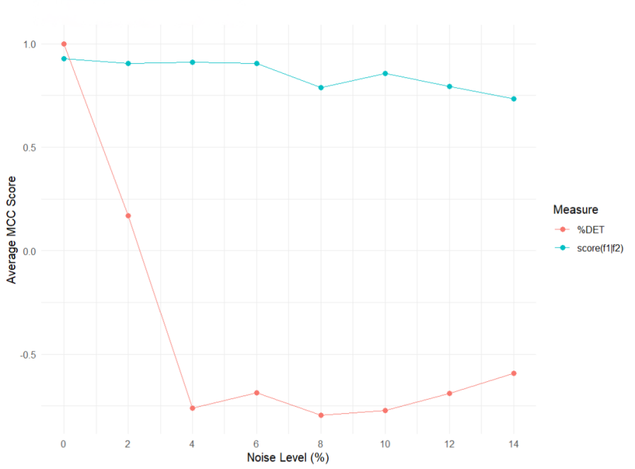
Figure 5: Average MCC scores for conditional periodicity score (blue) and percent determinism (red) of square wave signals with increasing Gaussian noise.

4.4 Measuring Similarity of Periodicities

For a different set of performance comparisons, we compare multiple similarity measures between a fixed $\displaystyle w_{1}$-periodic cosine signal $\displaystyle f_{1}$ and several $\displaystyle w_{2}$-periodic cosine signals $\displaystyle f_{2}$ as $\displaystyle w_{2}$ diverges from $\displaystyle w_{1}$. We set $\displaystyle w_{1}=3$ and increase $\displaystyle w_{2}$ from $\displaystyle w_{1}$ to $\displaystyle 15$, and store the conditional periodicity scores, percent recurrence (%REC), percent determinism, and the maximum diagonal line lengths (MDLs) of the cross-recurrence matrices corresponding to the embeddings of $\displaystyle f_{1}$ and $\displaystyle f_{2}$. Percent recurrence measures the proportion of cross-recurring states (ones) in the cross-recurrence matrix, $\displaystyle C$, and, MDL measures the length of the longest diagonal strip of cross-recurring states in $\displaystyle C$ [16]. We again handle noise by setting the tolerance for $\displaystyle C$ greater than five times the Gaussian standard deviation and applying a simple moving average to both series followed by a mean shifting procedure for the conditional SWE (see results above for an explanation).

We generate Figure 6 by again fixing the precision determining the embedding dimension for each series $\displaystyle f_{2}$ to $\displaystyle\epsilon=0.0005$, the number of discrete time points in both signals to $\displaystyle P=200$, the number of points in all embedded point clouds to $\displaystyle N=100$, and the width of the simple moving average window to $\displaystyle 19$ points. We compare plots of $\displaystyle\operatorname{score}(f_{1}|f_{2})$, %REC, %DET, and MDL against indices corresponding to the diverging periodicity of $\displaystyle f_{2}$. As the periodicities of $\displaystyle f_{1}$ and $\displaystyle f_{2}$ become less similar, $\displaystyle\operatorname{score}(f_{1}|f_{2})$ decreases as expected. At the same time, the phase-space embeddings of $\displaystyle f_{1}$ and $\displaystyle f_{2}$ become less-correlated, and therefore $\displaystyle C$ contains more randomly located ones that are less frequently located in diagonal strips (i.e., % REC increases and %DET decreases).

Our scoring function exhibits expected behavior in a more stable manner compared to cross-recurrence, as $\displaystyle\operatorname{score}(f_{1}|f_{2})$ decreases at a more consistent rate than %REC and %DET increase and decrease, respectively. As well, %DET decreases at a much slower rate as soon as any Gaussian noise is added to the input time series.

We again repeat this same experiment on dampened, sawtooth, and square wave signals and obtain similar stability results for the same. See Figures 7, 8, and 9 for these respective results. For sawtooth signals, as soon as any Gaussian noise is added, %DET starts to increase rather than decrease and overall is a much less stable correlation measure when compared to our scoring function. For square wave signals, we see that our score is much more stable than %DET and %REC when subject to changing Gaussian noise levels.

Figure 6: Comparing stability of conditional periodicity score to percent recurrence, percent determinism, and maximum diagonal line length of cosine signals for varying noise levels (NLs). The top two plots show $\displaystyle\operatorname{score}(f_{1}|f_{2})$ and %REC and the bottom two plots show %DET and MDL against diverging frequencies of $\displaystyle f_{2}$ from $\displaystyle f_{1}$, respectively.

Figure 7: Comparing stability of conditional periodicity score to percent recurrence, percent determinism, and maximum diagonal line length for dampened cosine signals of varying noise levels (NLs). The top two plots show $\displaystyle\operatorname{score}(f_{1}|f_{2})$ and %REC and the bottom two plots show %DET and MDL against diverging frequencies of $\displaystyle f_{2}$ from $\displaystyle f_{1}$, respectively.

Figure 8: Comparing stability of conditional periodicity score to percent recurrence, percent determinism, and maximum diagonal line length for sawtooth signals of varying noise levels (NLs). The top two plots show $\displaystyle\operatorname{score}(f_{1}|f_{2})$ and %REC and the bottom two plots show %DET and MDL against diverging frequencies of $\displaystyle f_{2}$ from $\displaystyle f_{1}$, respectively.

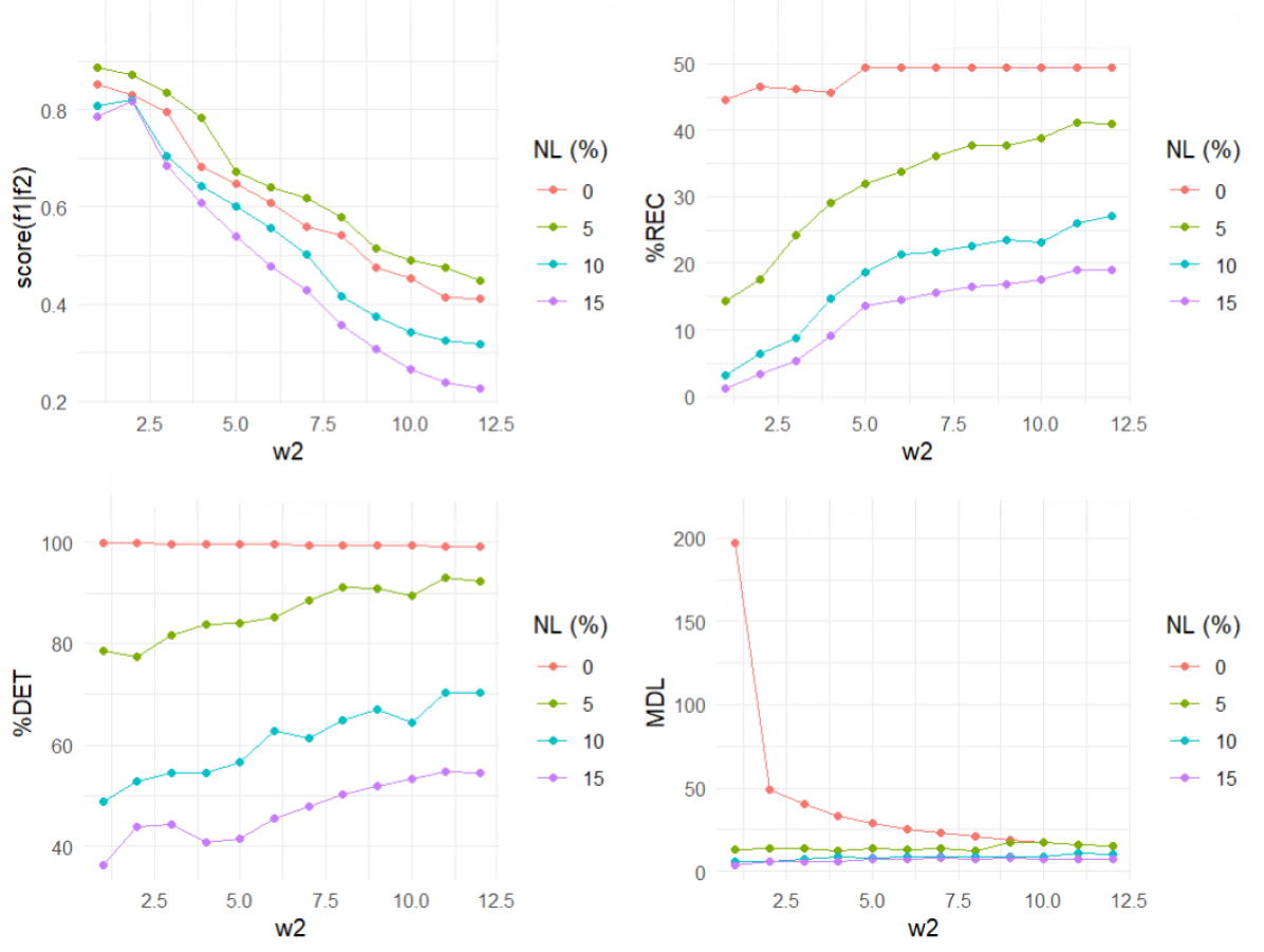
Figure 9: Comparing stability of conditional periodicity score to percent recurrence, percent determinism, and maximum diagonal line length for square wave signals of varying noise levels (NLs). The top two plots show $\displaystyle\operatorname{score}(f_{1}|f_{2})$ and %REC and the bottom two plots show %DET and MDL against diverging frequencies of $\displaystyle f_{2}$ from $\displaystyle f_{1}$, respectively.

5 Discussion

Our conditional periodicity score is a similarity measure that is not only comparable to other methods of quantifying similarity of univariate time series but also adds unique theoretical guarantees of stability under small changes in periodicity. As well, our score provides a direct measure of similarity between periodicity which others such as cross-correlation, coherence, and cross-recurrence are missing. Complementing the theoretical stability results, our score can be applied efficiently in practice with increased computational efficiency using PCA for dimension reduction. Our computations highlight the superior performance of the conditional periodicity score in predicting and measuring the closeness of periodicities when compared to cross-recurrence. While our measure provides a direct quantification of similarity that maintains theoretical stability, we are working on experimental results with real data, results when comparing pairs of synthetic series of different types; e.g., cosine vs square-wave or sawtooth vs dampened, and constructing a scoring function that quantifies the conditional periodicity of one univariate signal given a collection of others.

References

- [1] Henry Adams, Florian Frick, Sushovan Majhi, and Nicholas McBride. Hausdorff vs Gromov-Hausdorff distances, 2024. arXiv:2309.16648.
- [2] Luc Anselin. Dimension Reduction Methods (2): Distance Preserving Methods, 2020. Available as part of GeoDa: An Introduction to Spatial Data Science. URL: https://geodacenter.github.io/workbook/7ab_mds/lab7ab.html.
- [3] Eugene Oran Brigham and Richard E. Morrow. The fast Fourier transform. IEEE Spectrum, 4(12):63–70, 1967. doi:10.1109/MSPEC.1967.5217220.
- [4] Dmitri Burago, Yuri Burago, and Sergei Ivanov. A Course in Metric Geometry, volume 33 of Graduate Studies in Mathematics. American Mathematical Society, 2001.
- [5] Frédéric Chazal, Vin de Silva, Marc Glisse, and Steve Oudot. The Structure and Stability of Persistence Modules. SpringerBriefs in Mathematics. Springer Cham, 1 edition, 2016.
- [6] Frédéric Chazal, Vin de Silva, and Steve Oudot. Persistence stability for geometric complexes. Geometriae Dedicata, 173:193–214, 2014. doi:10.1007/s10711-013-9937-z.
- [7] Davide Chicco and Giuseppe Jurman. The advantages of the Matthews correlation coefficient (MCC) over F1 score and accuracy in binary classification evaluation. BMC Genomics, 21(16), 2020.
- [8] Dorin Comaniciu and Peter Meer. Mean shift: a robust approach toward feature space analysis. IEEE Transactions on Pattern Analysis and Machine Intelligence, 24(5):603–619, 2002. doi:10.1109/34.1000236.
- [9] Derek de Beurs, Erik J. Giltay, Chani Nuij, Rory O’Connor, Remco F.P. de Winter, Ad Kerkhof, Wouter van Ballegooijen, and Heleen Riper. Symptoms of a feather flock together? An exploratory secondary dynamic time warp analysis of 11 single case time series of suicidal ideation and related symptoms. Behaviour Research and Therapy, 178:104572, 2024. doi:10.1016/j.brat.2024.104572.
- [10] Shirley Duong, Tehran J. Davis, Heather J. Bachman, Elizabeth Votruba-Drzal, and Melissa E. Libertus. Dynamic structures of parent-child number talk: An application of categorical cross-recurrence quantification analysis and companion to Duong et al. (2024). The Quantitative Methods for Psychology, 20:137–155, 2024. doi:10.20982/tqmp.20.2.p137.
- [11] S.A. Dyer and J.S. Dyer. Cubic-spline interpolation. 1. IEEE Instrumentation & Measurement Magazine, 4(1):44–46, 2001. doi:10.1109/5289.911175.
- [12] Ian T. Jolliffe. Principal Component Analysis, volume 89. Springer-Verlag, 2002.
- [13] Andjelka B. Kovačević, Aleksandra Nina, Luka č Popović, and Milan Radovanović. Two-Dimensional Correlation Analysis of Periodicity in Noisy Series: Case of VLF Signal Amplitude Variations in the Time Vicinity of an Earthquake. Mathematics, 10(22), 2022. doi:10.3390/math10224278.
- [14] Musashi Ayrton Koyama, Facundo Memoli, Vanessa Robins, and Katharine Turner. Faster computation of degree-1 persistent homology using the reduced Vietoris-Rips filtration, 2024. arXiv:2307.16333.
- [15] Jean-Philippe Lachaux, Antoine Lutz, David Rudrauf, Diego Cosmelli, Michel Le Van Quyen, Jacques Martinerie, and Francisco Varela. Estimating the time-course of coherence between single-trial brain signals: An introduction to wavelet coherence. Neurophysiologie Clinique/Clinical Neurophysiology, 32(3):157–174, 2002. doi:10.1016/S0987-7053(02)00301-5.
- [16] Norbert Marwan, M. Carmen Romano, Marco Thiel, and J urgen Kurths. Recurrence plots for the analysis of complex systems. Physics Reports, 438(5):237–329, 2007. doi:10.1016/j.physrep.2006.11.001.
- [17] Brian W. Matthews. Comparison of the predicted and observed secondary structure of T4 phage lysozyme. Biochimica et Biophysica Acta (BBA) - Protein Structure, 405(2):442–451, 1975. doi:10.1016/0005-2795(75)90109-9.
- [18] Nathan H. May, Bala Krishnamoorthy, and Patrick Gambill. A Normalized Bottleneck Distance on Persistence Diagrams and Homology Preservation Under Dimension Reduction. La Matematica, pages 1–23, 2024. doi:10.1007/s44007-024-00130-0.
- [19] R. Mesbah, M. A. Koenders, A. T. Spijker, M. de Leeuw, A. M. van Hemert, and E. J. Giltay. Dynamic time warp analysis of individual symptom trajectories in individuals with bipolar disorder. Bipolar Disorders, 26:44–57, 2024. doi:10.1111/bdi.13340.
- [20] Jose Perea and John Harer. Sliding Windows and Persistence: An Application of Topological Methods to Signal Analysis. Foundations of Computational Mathematics, 15:799–838, 2015. arXiv:1307.6188, doi:10.1007/s10208-014-9206-z.
- [21] Jose A. Perea, Anastasia Deckard, Steve B. Haase, and John Harer. SW1PerS: Sliding windows and 1-persistence scoring; discovering periodicity in gene expression time series data. BMC Bioinformatics, 16(1):257, 2015. doi:10.1186/s12859-015-0645-6.
- [22] Christopher D. Riehm, Scott Bonnette, Justin L. Rush, Jed A. Diekfuss, Moein Koohestani, Gregory D. Myer, Grant E. Norte, and David A. Sherman. Corticomuscular cross-recurrence analysis reveals between-limb differences in motor control among individuals with ACL reconstruction. Experimental Brain Research, 242:355–365, 2024. doi:10.1007/s00221-023-06751-1.
- [23] Floris Takens. Detecting strange attractors in turbulence. In David Rand and Lai-Sang Young, editors, Dynamical Systems and Turbulence, Warwick 1980, pages 366–381, Berlin, Heidelberg, 1981. Springer Berlin Heidelberg.
- [24] Christopher J. Tralie and Jose A. Perea. (Quasi)Periodicity Quantification in Video Data, Using Topology. SIAM Journal on Imaging Sciences, 11(2):1049–1077, 2018. doi:10.1137/17M1150736.
- [25] Sarah Tymochko, Elizabeth Munch, Jason Dunion, Kristen Corbosiero, and Ryan Torn. Using persistent homology to quantify a diurnal cycle in hurricanes. Pattern Recognition Letters, 133:137–143, 2020. doi:10.1016/j.patrec.2020.02.022.
- [26] Zhaokun Wei, Yaning Gao, Xiaoju Zhang, Xiaojun Li, and Zhifeng Han. Adaptive marine traffic behaviour pattern recognition based on multidimensional dynamic time warping and DBSCAN algorithm. Expert Systems with Applications, 238:122229, 2024. doi:10.1016/j.eswa.2023.122229.
- [27] Hasan Yiǧit. Time Complexity of PCA 1. General Time Complexity of PCA, 08 2024. Posted on ResearchGate. doi:10.13140/RG.2.2.12847.34728.
- [28] Yang Zhan, David Halliday, Ping Jiang, Xuguang Liu, and Jianfeng Feng. Detecting time-dependent coherence between non-stationary electrophysiological signals: A combined statistical and time-frequency approach. Journal of Neuroscience Methods, 156(1):322–332, 2006. doi:10.1016/j.jneumeth.2006.02.013.
- [29] Wei Zhang, Satar Bakhsh, Kishwar Ali, and Muhammad Anas. Fostering environmental sustainability: An analysis of green investment and digital financial inclusion in China using quantile-on-quantile regression and wavelet coherence approach. Gondwana Research, 128:69–85, 2024. doi:10.1016/j.gr.2023.10.014.
- [30] Afra Zomorodian and Gunnar Carlsson. Computing Persistent Homology. Discrete & Computational Geometry, 33(2):249–274, February 2005. doi:10.1007/s00454-004-1146-y.