From Dense to Sparse: Event Response for Enhanced Residential Load Forecasting

Abstract

Residential load forecasting (RLF) is crucial for resource scheduling in power systems. Most existing methods utilize all given load records (dense data) to indiscriminately extract the dependencies between historical and future time series. However, there exist important regular patterns residing in the event-related associations among different appliances (sparse knowledge), which have yet been ignored. In this paper, we propose an Event-Response Knowledge Guided approach (ERKG) for RLF by incorporating the estimation of electricity usage events for different appliances, mining event-related sparse knowledge from the load series. With ERKG, the event-response estimation enables portraying the electricity consumption behaviors of residents, revealing regular variations in appliance operational states. To be specific, ERKG consists of knowledge extraction and guidance: i) a forecasting model is designed for the electricity usage events by estimating appliance operational states, aiming to extract the event-related sparse knowledge; ii) a novel knowledge-guided mechanism is established by fusing such state estimates of the appliance events into the RLF model, which can give particular focuses on the patterns of users’ electricity consumption behaviors. Notably, ERKG can flexibly serve as a plug-in module to boost the capability of existing forecasting models by leveraging event response. In numerical experiments, extensive comparisons and ablation studies have verified the effectiveness of our ERKG, e.g., over 8% MAE can be reduced on the tested state-of-the-art forecasting models. The source code will be available at https://github.com/ergoucao/ERKG.

I Introduction

Residential Load Forecasting (RLF) aims to predict future electricity usages for individual consumers, reflecting their anticipated household power demands and the corresponding electricity consumption behaviors. In the power systems, different participants can be benefited from the forecast analysis of electricity usage . For the system operator, RLF can provide an aggregated future power demand of residents within a certain area. Based on the current electricity resource situation and power demands, the operator formulates corresponding power dispatch or demand response strategies. For example, by adopting varied Time-of-Use pricing schemes, consumers can dynamically adjust their electricity usage to achieve peak shaving and valley filling for power grid [1]. For the consumer, RLF enables better residential scheduling to cope with Real-Time Pricing or to determine the energy storage in advance [2]. Accurate RLF facilitates an optimal allocation of power resources for boosting the efficiency and reliability of the power systems, and thus has been becoming a popular research field within both the industrial and academic communities.

Smart meters deployments and Non-Invasive Load Monitoring advancements have provided accesses to extensive fine-grained data [3, 4], laying the groundwork for accurate analysis of residential user behaviors. On such bases, many studies have been proposed to explore the inherent dependencies in massive historical data [5, 6, 7, 8, 9, 10, 8], e.g., series historical seasonality and growth patterns. Most existing RLF approaches can generally be categorized into two groups based on the forecasting levels, i.e., household level and appliance level. Specially, household-level methods aim at forecasting the total electricity usage for the entire household. In [5, 6], the RLF models address to capture the temporal dependencies from historical load series, while [7, 8] utilize spatial correlations among multiple households to enhance RLF. Appliance-level methods focus on predicting the energy usage of electrical devices within a household, exploiting the relationship between electricity consumption habit of resident and appliance electricity usage. RALF-LSTM [9] proposes a recurrent deep neural network that considers the energy-saving behavior of individual users for estimating future appliance energy usage. To improve the model capability, ALSTLF-RNN [10] leverages the similarity in energy consumption patterns among appliances across different households. In [6], Kong et al. claim the mutual relationship between the appliance-level and household-level, and the relationship contributes to RLF. Forecasting at both levels explicitly facilitates learning this mutual relationship. In fact, RLF at two levels constitutes a Multivariate Time Series Forecasting (MTSF) problem. This involves both identifying intra-variable historical patterns and modeling inter-variable relationships to reflect consumer electricity usage. However, the electricity usage patterns at the appliance-level and house-level are typically different, and their relationship is also dynamic [11].

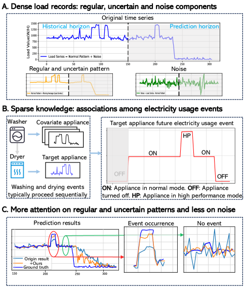
Figure 1: The illustration of the proposed approach ERKG: Learning event-related sparse knowledge from dense data, enabling model focus on the electricity consumption behaviors in reality, i.e., regular and uncertain patterns. Specifically, (A): The original dense load series consist of regular and uncertain patterns, as well as noise, which impact predictive performances. (B): By learning the intrinsic relationship between future electricity usage events and historical load records, ERKG extracts sparse knowledge, i.e., event-related sparse knowledge, which is represented by class probabilities of appliance operational states. (C): The use of sparse knowledge guides the prediction model to focus on regular and uncertain patterns, reducing noise fitting. In practice, we utilize appliance operational states class probabilities as weights to regularize the training loss of the prediction model.

Recent progresses in MTSF have yielded advanced models skilled in managing complex intra-variable and inter-variable patterns, notably falling into Transformer-based and MLP-based categories. Transformer-based models capture long-term dependency with self-attention, using positional encoding techniques to preserve temporal information[12, 13, 14, 15]. In particular, Autoformer[13] proposes an Auto-Correlation mechanism based on the series periodicity, which utilizes dependencies discovery at the sub-series level to learn complex temporal patterns. ETSformer [14] models series patterns by decomposing the series into interpretable components such as level, growth, and seasonality. Crossformer[15] employs a dimension-segment embedding to comprehensively learn relationships between series variables. On the other hand, MLP-based models retain complete temporal information with default linear architecture. For instance, LTSF-Linear[16] can be comparable to most of the previously mentioned Transformer-based models. This work has empirically validated that the linear model effectively retains temporal information. Meanwhile, IBM and Google have introduced MLP-Mixer models [17, 18], further improving the performance of MLP-based models. The aforementioned work indiscriminately learns all inherent patterns in given time series, assuming that the model can automatically utilize these inherent patterns for prediction.

However, residential load series blend normal patters with corruption patterns, as shown in Fig. 1. A: $i$) the regular and uncertain patterns (normal patterns), which represent electricity consumption behaviors; and $ii$) the noise or anomalous disturbances (corruption patterns), potentially caused by instability and aging of appliances and measurement devices; it can clearly observed that compared to corruption patterns, the variations in normal patterns are sparse. Due to the patterns bias, these indiscriminate learning approaches, i.e., directly modeling the series value-level relationship between historical and future time series, often result in under-exploration of normal patterns and overfitting of corruption patterns, leading to insufficient performance in RLF.

We consider focusing on exploring the normal patterns based on event-related sparse knowledge, which represents the event relationships among different appliances. As shown in Fig. 1. B, it illustrates a novel pattern learning paradigm in RLF, which utilizes historical load records to estimate future events. Specifically, due to the cleaning habits of users, washing and drying events occur sequentially (event-related sparse knowledge). Based on this associations, when the washer (the covariate appliance) is consuming electricity and the dryer (the target appliance) is still not in operation, we can estimate the future electricity usage event of dryer, i.e., transitioning from state “OFF” $\Rightarrow$ “ON” $\Rightarrow$ … $\Rightarrow$ “OFF”. This paradigm can effectively extract event-related sparse knowledge and concentrate on the normal patterns in load series.

In this work, we propose ERKG, a Event-Response Knowledge Guided approach to enhance RLF models in performing both household level and application level load forecasting. To be specific, ERKG consists of knowledge extraction and guidance: i) for extraction, this paper propose an event estimation paradigm, it is a multivariate state predictor that forecasts the future appliance operational states based on historical load series, and specifically models the state changes of appliances to learn event-related sparse knowledge; ii) for guidance, this paper develops a knowledge guide mechanism based on event response to fuse event-related knowledge into the RLF model. Notably, ERKG can flexibly serve as a plug-in module to enhance the concentration of RLF model training on key areas, i.e., event occurrence in Fig. 1. C, without changing the model’s structure and inference process. Finally, experiments on three datasets with three state-of-the-art prediction models demonstrate a 8% improvement in Mean Absolute Error (MAE), affirming the effectiveness of ERKG. The main contributions of this work are summarized as follows.

1. We propose an event response knowledge-guided approach to address the challenge of exploiting event-related sparse knowledge from the given load records (dense data) for RLF.

2. For event-related sparse knowledge extraction, an forecasting model is designed for electricity usage events by estimating the operational states of appliances, obtaining event-related associations from historical load series.

3. With such event-related sparse knowledge, a novel knowledge-guided mechanism is constructed by leveraging event response to promote the learning of regular and uncertain patterns that are beneficial for forecasting.

4. Extensive numerical experiments have been conducted to evaluate the proposed ERKG on widely used residential datasets, showing that ERKG notably enhances the performance of existing state-of-the-art forecasting models as a plug-in module.

The remainder of this work is organized as follows. Section II presents the related works. The problem definition is elaborated in Section III. Section IV introduces the proposed method. Section V gives experimental results. We conclude our work with outlooks in Section VI.

II RELATED WORK

II-A Residential Load Forecasting

The residential load is a typical type of time series, for which many forecasting methods have been proposed, involving traditional statistical and machine learning techniques, where deep learning methods are currently of popularity. Traditional statistical methods can learn linear or simple nonlinear relations in data through linear combinations of historical data, e.g., the AutoRegressive Integrated Moving Average (ARIMA) method. Specifically, CSTLF-ARIMA [19] integrates the ARIMA model and the transfer function to improve model prediction accuracy, where the relations between weather and load are taken into account. RLF-IGA [20] employs an integrated Gaussian process that leverages associations from both target and related customers for reliable hourly residential load prediction. Through specialized feature engineering techniques, machine learning methods can handle more complicated nonlinearity in data, e.g., Support Vector Regression (SVR) machines. MFRLF-SVR [21] uses SVR to investigate the impact of temporal granularity on model accuracy, suggesting that the optimal granularity is hourly. HFSM [22] proposes a holistic feature selection method, boosting ANN-based forecasting model. In particular, recent advancements show that deep learning methods are highly effective in capturing complex patterns residing in time series. Particularly, Long Short-Term Memory [5] leverages recurrent network structures to retain complex temporal patterns. Meanwhile, many methods propose model spatial relationships among residential load series, e.g., the relations among residential users [7, 8] and the associations between appliances [9, 10]. It is worth noting that the electrical appliance load plays a positive role in household load forecasting [6]. However, only a few studies have analyzed the electrical characteristics of appliances. For instance, MTL-GRU [4] categorizes appliances into continuous and intermittent load appliances and employs different methods for processing them. Meanwhile, Welikala et al. [23] incorporate appliance usage patterns (AUPs) for NILM and load forecasting. Their approach is based on pre-observed AUPs to obtain the prior probabilities of appliances being activated (“ON”), resulting in more accurate NILM and load forecasting results.

Our ERKG leverages an electricity usage event forecasting model that learns not only complex intra-variable patterns, e.g., changes in appliance usage patterns over different times, but also inter-variable patterns, e.g., relationships between different appliances. Specifically, different from these work [4, 24] that focuses on the characteristics of individual appliances or the combination of activity/inactivity of appliances [23], our work considers the event-related associations among appliances with multiple different appliance operating states to enhance state-of-the-art MTSF models for RLF.

II-B Knowledge Guided Deep Learning

Deep learning methods have been proven powerful in various areas, such as computer vision and recommending systems. However, when special scenario events occur, such as traffic flow under inclement weather and accidents, relying solely on the given raw data can make it difficult to discover important factors and learn complex data relationships. Thus, the resulting performances can still be limited, depite of the great model capacity of deep learning methods. Some existing work [25, 26, 27, 28, 29] propose to utilize prior knowledge to guide the learning process. Yin et al. [26] use accumulated medical knowledge from large public datasets to compensate for data in clinical car, while Peng et al. [27] utilize context information from events, e.g., accidents, and environmental factors, e.g., weather, to construct knowledge graph that guide the learning of traffic flow predictors. These methods can be categorized into two types, depending on the utilization of external knowledge or internal model knowledge.

For the methods based on external knowledge, the performances are enhanced by learning more specific domain data. Kerl [30] is a knowledge-guided reinforcement learning model that integrates knowledge graph information for sequential recommendation, facilitating the handling of sparse and complex user-item interaction data. Peng et al. [27] demonstrate using knowledge and situational awareness, i.e., weather and traffic data, to improve model performance under conditions such as severe traffic accidents. Yin et al. [26] propose a domain knowledge-guided network that utilizes the causal relationships among clinical events to improve modeling accuracy. These approaches require custom embedding and design of the original model based on specific knowledge, limiting their extensibility.

For the methods based on internal model knowledge, the learning relies on utilizing knowledge from auxiliary models. In particular, to improve the efficiency of knowledge-guided teacher-student (auxiliary-target) learning, Hinton et al. [31] introduce response-based knowledge, i.e., soft targets, for image classification, which preserves the probabilistic relationships among different categories. Considering task-specific knowledge in multi-task recommendation, Yang et al. [32] propose a cross-task learning framework that uses response-based knowledge contained in auxiliary tasks. Response-based knowledge guide methods are simple yet effective, which directly utilize logits regularization to make the student (target) model mimic the neural response of the teacher (auxiliary) model. The logits regularization loss does not affect the structure and inference of the target model. The proposed ERKG is an event response-based method that can serve as a plug-in module. Unlike the above response-based methods, we use event-related sparse knowledge to construct conditional targets to guide the target model in identifying and focusing on key patterns within the data.

III Problem Definition

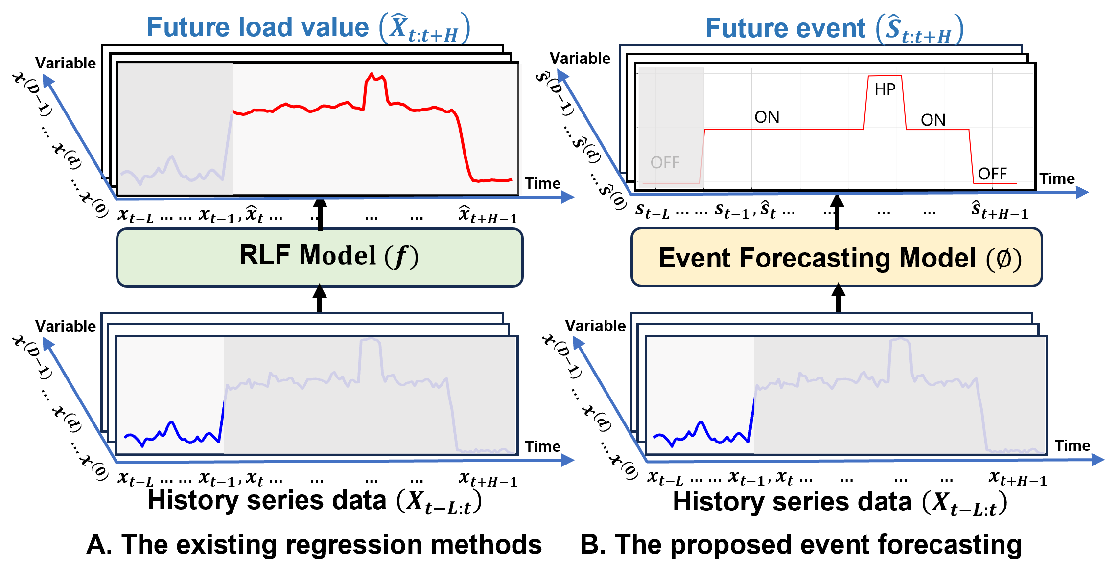
Figure 2: Two learning paradigms. (A): Existing methods directly predict future loads using historical load values. (B): Our event forecasting method estimates appliance operational states using historical load values and models the state changes of appliances to learn event-related sparse knowledge.

Our approach involves conducting RLF at both household level and application level simultaneously. Let $x_{t}=[x_{t}^{(0)},\dots,x_{t}^{(D-1)}]$ denote an observation of household and appliances load series at time step $t$, where $D$ equals of smart meters, including measuring devices for appliances and household rooms. As shown in Fig. 2. A, given a lookback window $X_{t-L:t}=[x_{t-L},\dots,x_{t-1}]$, we consider the task of predicting future $H$-length time steps, $X_{t:t+H}=[x_{t},\dots,x_{t+H-1}]$. We denote $\hat{X}_{t:t+H}$ as the point forecast of $X_{t:t+H}$. Thus, the goal is to learn a forecasting function $f$ by minimizing some loss function $\mathcal{L}:\mathbb{R}^{H\times D}\times\mathbb{R}^{H\times D}\to\mathbb{R}$, as shown in Eq. (1):

$$\hat{X}_{t:t+H}=f(X_{t-L:t}).$$ (1)

In previous work, load values are often treated as single entities, and modeling these values is considered as a regression task. For example, VAE-LF [33] utilizes a variational autoencoder-based regression model to describe the local relationship between historical aggregated load values and future target appliance values, with the target appliances including manually pre-selected ones, i.e., Washing Machine, Dishwasher, and Fridge. However, regression-based methods, along with the corresponding loss function such as MSE, face limitations. Notably, due to the double penalty issue[34], they tend to produce conservative forecasts for future load curves[35], which may overlook event-related knowledge. To overcome this limitation, as shown in Fig. 2. B, we transform continuous load values into states for predicting appliance operational states. This task is inherently a multi-task forecasting problem due to the concurrent operations of multiple appliances. Different from VAE-LF that employing a prediction of future load values as an estimation of operational states, our ERKG first identifies the various multi-states of different appliances through adaptive clustering and then overviews historical data to predict future states as a description of electricity usage events.

Let $x^{(i)}=[x_{0}^{(i)},\dots,x_{l-1}^{(i)}]$ denote the load series for the i-th variable where $i\in{\{0,\dots,D-1\}}$, $l$ equals the origin series length, and $n_{x^{(i)}}$ represents the number of operation states for variable $x^{(i)}$, e.g., $n_{\rm{dryer}}$ equals three in Fig. 1. B: “OFF”, “ON” and “HP”. We define $s_{t}\in\mathbb{R}^{D}$ as the state for $x_{t}$, with each $s_{t,i}\in{\{0,\dots,n_{x^{(i)}}-1\}}$ corresponding to $x_{t}^{(i)}$. Likewise, given a lookback window $X_{t-L:t}$, and a set of operation state numbers $N_{0:D}=\{n_{x^{0}},\dots,n_{x^{D-1}}\}$, $\hat{S}_{t:t+H}$ denotes the forecast of the state $S_{t:t+H}=[s_{t},\dots,s_{t+H-1}]$, obtained by minimizing the cross-entry loss function. The state forecasting function $\phi$ is defined in Eq. (2):

$$\hat{S}_{t:t+H}=\phi{\left(X_{{t-L}:t}\right)}.$$ (2)

Eq. (1) and Eq. (2) represent two learning paradigms, as shown in Fig. 2. In contrast to Eq. (1), learning directly from the series value-leve (Fig. 2. A), Eq. (2) is a new paradigm that models electricity consumption behaviors through electricity usage events, which facilitates RLF (Fig. 2. B).

Figure 3: Left Penal: The paradigm of existing methods, e.g., Crossformer[15], ETSformer[14] and TSMixer[18]. They directly model series value-level relationship between history and future. Right Penal: The overview of the proposed ERKG Approach. It can enhance the performance of existing methods through the estimation of electricity usage events for different appliances

IV METHODOLOGY

In this section, a novel knowledge guided approach for RLF introduced, namely ERKG, which gives particular considerations to event-related sparse knowledge from the given dense load records and meanwhile avoids the overfitting to noise. As illustrated in Fig. 3, ERKG consists of two main parts, i.e., a electricity usage events forecasting model and a knowledge-guided mechanism based on event response. The former exploits event-related sparse knowledge; the latter utilizes such sparse knowledge to extract the key patterns residing in the data and meanwhile to reduce attention on noises. Notably, ERKG can be flexibly plugged into various RLF models, such as Crossformer, Etsformer, and TSMixer, as explained in IV-C.

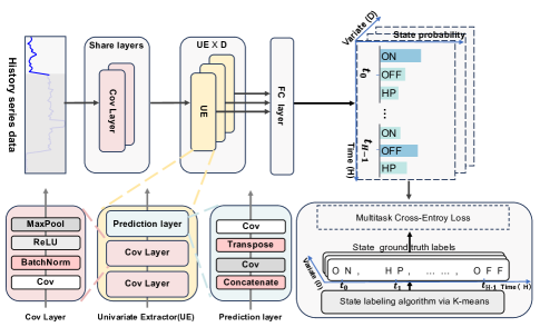
Figure 4: The proposed electricity usage events forecasting model.

IV-A Electricity Usage Event Forecasting Model

For event-related sparse knowledge extraction, the electricity usage events forecasting model estimates appliance operational states, focusing on event-related associations in historical load series by training the Multivariate State Predictor (MSP) to predict the probability of future electricity usage events. As shown in Fig. 4, it includes the state predictor and the state labeling algorithm: $i)$ a Multivariate State Predictor (MSP) is created to predict the future state class probabilities of series, e.g., “ON”, “OFF”, and “HP” ; $ii)$ a state labeling algorithm uses $k$-means to obtain the corresponding state ground truth labels, which facilitates the predictor in learning sparse knowledge.

IV-A1 Multivariate State Predictor

The MSP processes historical multivariate load series values to predict the corresponding future multi-step series state class probabilities. It processes $D$ variates and an $L$-length load series $X_{t-L:t}=\{X_{t-L:t}^{(i)}\mid i\in\{0,1,\dots,D-1\}\}$ to produce an $H$-length load state series $\hat{S}_{t:t+H}=\{\hat{S}_{t:t+H}^{(i)}\mid i\in\{0,1,\dots,D-1\}\}$. The MSP consists of three components in sequence: Shared layers, $D$ Univariate Extractors (UE), and a Fully Connected (FC) layer, denoted as $\phi_{sl}$ , $\phi_{u}=\{\phi_{u^{(i)}}\mid i\in\{0,1,\dotsc,D-1\}\}$, $\phi_{fc}$, respectively. Specifically, $\phi_{sl}$ extract low-level information, and $\phi_{u^{(i)}}$ is responsible for independent state predictions with $X_{t-L:t}$, such that:

$$Z_{u}^{(i)}=\phi_{u_{x^{(i)}}}{(\phi_{sl}(X_{t-L:t}))},\text{ for }i\in\{0,1,\ldots,D-1\},$$ (3)

where $Z_{u}^{(i)}$ is the probability score distributions of univariate $x^{(i)}\in\mathbb{R}^{H\times n_{x^{(i)}}}$, and $n_{x^{(i)}}$ equals the number of appliance operation states for variable $x^{(i)}$. Aligned with the feature processing of data in [36], we use one-dimensional (1-$D$) convolution to construct the Prediction layer in UE.

Concerning the connections among appliance states, we apply $\phi_{fc}$ to integrate their correlations as in Eq.(4):

$$Z=\phi_{fc}(Z_{u}),$$ (4)

where we concatenate all $Z_{u}^{(i)}$ to obtain $Z_{u}$ $\in\mathbb{R}^{H\times\sum_{i=0}^{D-1}{n_{x^{(i)}}}}$ and pass $Z_{u}$ through $\phi_{fc}$ to get $Z\in\mathbb{R}^{H\times\sum_{i=0}^{D-1}{n_{x^{(i)}}}}$.

We then split $Z$ into $D$ group probability score distributions $\{Z^{(i)}\mid i\in\{0,1,\dots,D-1\}\}$ to calculate the state category for each variable. In fact, the MSP concludes $\hat{S}_{t:t+H}=\{\hat{S}_{t:t+H}^{(i)}\mid i\in\{0,1,\dots,D-1\}\}$ with maximum probability score $Z^{(i)}$. We thereby consider the load state of each variable at each time step as follows:

$$\hat{s}_{\tau}^{(i)}=\mathop{\arg\max}\nolimits_{c}{z^{\tau,i,c}},\text{ for }c\in\{0,1,\dotsc,n_{x^{(i)}}\},$$ (5)

where $\hat{s}_{\tau}^{(i)}$ is the load state of the $i$-th variable at time step $\tau$, and $z^{\tau,i,c}$ is the score of the corresponding $c$-th state. Let $\hat{S}_{t:t+H}^{(i)}=\{\hat{s}_{\tau}^{(i)}\mid\tau\in\{0,1,\dots,H-1\}\}$, and we have the $H$-length load state series $\hat{S}_{t:t+H}=\{\hat{S}_{t:t+H}^{(i)}\mid i\in\{0,1,\dots,D-1\}\}$ for all $D$ variables $X_{t-L:t}$.

For MSP, we use a softmax function for normalization, and then choose multitask cross-entropy as our loss function $\mathcal{L}_{\rm MSP}$, which is defined as:

$$p_{\tau,i,c}=\frac{e^{z_{\tau,i,c}}}{\sum_{\ell=0}^{n_{x^{(i)}}-1}{e^{z_{\tau,i,\ell}}}},$$ (6)

$$\mathcal{L}_{\rm MSP}=\frac{1}{H}\sum_{\tau=t}^{t+H-1}\frac{1}{D}\sum_{d=0}^{D-1}-\log({p_{\tau,i,s_{\tau}^{(i)}}}),$$ (7)

where $p_{\tau,i,c}$ is the probability score for the $c$-th category of the $i$-th variable at future time step $\tau$, calculated using the softmax function, $H$ is the number of forecasting time steps, $D$ is the number of dimension variables, and $s_{\tau}^{(i)}\in\{0,1,\dots,n_{x^{(}i)}\}$ is the state ground truth label obtained by State Labeling Identification Algorithm for the $i$-th variable at time step $\tau$.

IV-A2 State Labeling Identification Algorithm

The state identification algorithm aims to address the issue of obtaining the state class of series values by performing an overall analysis of the load series. In fact, to train the MSP effectively, we utilize $k$-means clustering[37] to categorize the original series values into distinct states[38], forming the state ground truth labels $S\in{\mathbb{R}^{l\times{D}}}$. Here, $N_{0:D}$ denotes number of state categories. Specifically, given the original load series $\mathcal{E}\in\mathbb{R}^{l\times D}$, where $l$ is the length of time step and $D$ represents the variable dimensionality of load series (indicative of the number of appliances and rooms). We employ sliding windows of size $w$ to generate samples and set the bounds for clustering states as $min_{s}$ and $max_{s}$, referring to the existing studies[39, 40] on the number of appliance operational states, we set $min_{s}$ to 2 and $max_{s}$ to 5. Then, the $k$-means clustering is applied to each variable, where the optimal number of clusters $k_{\text{max}}$ is determined as the final state number $N_{0:D}$ based on the silhouette score[41], as presented in Algorithm 1.

Algorithm 1 State Labeling Identification via Time Series Clustering

1:Input: origin load series $\mathcal{X}$; origin load time length $l$; The variables dimension of load series, $D$; windows size $w$, state minimum $min_{s}$, state maximum $max_{s}$

2:Output: State Profile $S$

3:$\mathcal{E}\leftarrow\textsc{ZeroMatrix}(l,w,D)$

4:for $t\in\{0,\ldots,l-w\}$ do

5:  $\mathcal{E}[t]\leftarrow\mathcal{X}[t:t+w]$

6:end for

7:for $t\in\{l-w+1,\ldots,l\}$ do

8:  $\mathcal{E}[t]\leftarrow\mathcal{X}[t-w:t]$

9:end for

10:$S\leftarrow\textsc{ZeroLike}(\mathcal{X}),N\leftarrow\textsc{ZeroMATRIX}({D})$

11:for $i\in\{1,\ldots,D\}$ do

12:  $M_{\text{max}},S_{\text{max}},k_{\text{max}}\leftarrow 0,\text{nil},\text{nil}$

13:  for $k\in\{min_{s},\ldots,max_{s}\}$ do

14:   $s\leftarrow\textsc{TimeSeriesKMeans}(n).\textsc{Fit}(\mathcal{E}[:,:,i])$

15:   $m\leftarrow\textsc{SilhouetteScore}(\mathcal{E}[:,:,i],s)$

16:   if $m>m_{\text{max}}$ then

17:     $m_{\text{max}},s_{\text{max}},k_{\text{max}}\leftarrow m,s,k$

18:   end if

19:  end for

20:  $S[:,i],N[i]\leftarrow s_{\text{max}},k_{\text{max}}$

21:end for

22:Output($S$, $N$)

IV-B Knowledge-Guided Mechanism Based on Event Response

Based on event response, we propose a knowledge-guided mechanism to guide the RLF model with more attention on normal patterns of the load series and less sensitivity to the corrupted patterns, thereby enhancing the model prediction performances. More specifically, this mechanism employs event-related knowledge to enable the RLF model to identify and focus on informative event-related patterns. We use the values of the multi-step series state class probabilities as weights (indicating event-related knowledge) to regularize the traditional MAE or MSE training loss, through a specifically designed Teacher-Student (T-S) learning process. For example, more loss penalties on key areas, while less on areas that may contain noise. Notably, a key area can be the place where the state changes (event occurrence) , which can be observed in the comparison between the difference distribution and enhanced difference distribution shown in Fig. 3.

In particular, we design a Teacher-Student (T-S) learning process to transfer event-related knowledge from a MSP (Teacher) to the RLF model (Student). In the T-S process, the response-based knowledge usually refers to the neural response of the last output layer of the teacher model. The main idea is to let the Student model directly mimic the final prediction of the Teacher model. Given a vector of logits $Z$ as the outputs of the last output layer of a deep model, the loss for response-based knowledge can be formulated as

$$L_{Res}(Z_{t},Z_{s})=\mathcal{L}_{R}(Z_{t},Z_{s}),$$ (8)

where $\mathcal{L}_{R}$ indicates the divergence loss of logits, and $Z_{t}$ and $Z_{s}$ are logits of Teacher and Student, respectively. Different from the general response-based knowledge transfer in T-S process, we utilize the MSP to guide the Student to focus on key area of learning through $Z_{t}$, instead of directly having the Student mimic the Teacher. Moreover, our Teacher and Student have different forms outputs. Therefore, we design a response-based event-related knowledge loss as

$$\mathcal{L}_{\rm Res}(Z_{t},\hat{Y},Y)=\mathcal{L}_{\rm PR}(\hat{Y},Y|Z_{t}),$$ (9)

where the $\mathcal{L}_{\rm PR}$ indicates the error between the predicted and actual values in the space specified by the $Z_{t}$ logit. Specifically, we denote $Z_{t}$ as $Z$, with the logits $Z$ in Eq.(4) we define $\mathcal{L_{\rm PR}}$ as

$$\mathcal{L}_{\rm PR}=\frac{1}{D}\sum_{i=0}^{D-1}\frac{1}{H}\sum_{j=t}^{t+H}{{\max(Z_{j}^{(i)})}|\hat{Y}_{j}^{(i)}-Y_{j}^{(i)}|},$$ (10)

$$\mathcal{L}_{\rm MAE}=|\hat{Y}-Y|,$$ (11)

$$\mathcal{L}=\mathcal{L}_{\rm MAE}+\alpha\mathcal{L}_{\rm PR},$$ (12)

where $\hat{Y}_{j}^{(i)}$ and $Y_{j}^{(i)}$ are respectively predicted and actual values at the $j$-th time step and $i$-th dimension variable, $H$ represents the number of forecasting time steps, and $D$ represents the number of dimension variables. The maximization operation on $(Z_{j}^{(i)})$ acts as a weight emphasizing the key area in the learning process. $\mathcal{L}_{\rm PR}$ indicate the $Z$ of MSP specifies a weight on different time step and dimension, it encourage the model to focus on key area. $\mathcal{L}_{\rm MAE}$ is a general regression loss, and $\mathcal{L}$ is the final loss to train the RLF model.

IV-C Integration as a Plug-in Module to RLF Models

Our proposed ERKG can be flexibly plugged into most neural network methods for multi-step time series forecasting with regression losses, such as Mean Absolute Error (MAE), Mean Squared Error (MSE). Firstly, as introduced in Section III.A, we utilize the State Labeling Identification Algorithm to obtain state ground truth labels that indicate event information, and we train the electricity usage events forecasting model end-to-end using these labels. Secondly, the RLF model training process is guided by a knowledge-guided mechanism based on event response, as detailed in Section III.B, to enhance the predictive performance. The enhancing procedure is presented in Algorithm 2.

Algorithm 2 Enhancing Procedure

1:Input: Input series $X_{{t-L}:t}$ for MSP $\phi$, max_epochs, hyperparameters $\alpha$

2:Output: RLF model $f$

3:Initialize model parameters: $\phi$, $f$

4:Stage 1: train the MSP

5:Get state ground truth labels $S$ by algorithm 1

6:repeat

7:  for $t\in\{1,\ldots,T\}$ do

8:   Obtain $\hat{S}_{t:t+H}$ from $\phi$ for input $X_{{t-L}:t}$

9:   Compute the MSP loss $L_{\text{MSP}}$ (Eq. 7) with $S_{t:t+H}$

10:   Update the parameters of $\phi$ using $L_{\text{MSP}}$

11:  end for

12:until converge

13:Stage 2: Knowledge-guided RLF model training process

14:repeat

15:  for $t\in\{1,\ldots,T\}$ do

16:   Fix $\phi$ and input $X_{{t-L}:t}$ to obtain $Z=\phi(X_{{t-L}:t})$

17:   Compute the knowledge-guide loss $L$ using Eq. 12

18:   Update the parameters of $f$ using $L$

19:  end for

20:until converge

21:return enhanced model $f$

V Experiments and Discussions

V-A Datasets

In the experiments, we evaluate the proposed method on three publicly available and actual residential load datasets, i.e., Ampds2[42], UK-Dale[43], and UMass Smart Home[44]. They encompass both household-level aggregated and appliance-level disaggregated power data. More descriptions of the three datasets are summarized in Table I.

Almanac of Minutely Power Dataset [42]

AMPds2 collected energy consumption data of a residential house with 20 appliances and weather data in Canada from April 2012 to April 2014. It contains a total of 1,051,200 readings from two years of monitoring per meter.

UK Domestic Appliance-Level Electricity Dataset [43]

UK-Dale is an open-access dataset from the UK recording domestic appliance-level electricity. UK-Dale contains data for five actual residential houses in the UK, and we use the data from household 1 for the experiment, which was recorded for 655 days, and 47 dimension measure result.

UMass Smart Home Dataset [44]

Multiple smart meter readings of 7 homes were collected by the UMass Smart Home project in the US from 2014 to 2016, containing readings from separate smart meters controlling different appliances, where we choose houses C and D for the experiments.

Before training, a uniform preprocessing procedure has been performed on each dataset. Firstly, we align the start and end times of all measurement series within the same house, including both household-level and appliance-level. We also utilize downsampling to standardize the sampling period of series to 1 hour, meaning that each time point interval in the input model samples is 1 hour. Then, through the process of algorithm 1 for state labeling identification, the state data for all series are obtained. Finally, 60% of the data are used for training, 20% are used for validation, and the remaining 20% are used for testing. The data were normalized using the mean and standard deviation values computed from the training set.

TABLE I: Descriptions of the datasets

Dataset	Range	Sample Rate	Dimension
Ampds2	2012/4/01-2014/4/01	1 minute	23
UK-DALE	2013/4/11-2014/12/23	1 minute	47
UmassC	2016/1/01-2016/12/15	1 minute	22
UmassD	2016/1/01-2016/12/31	1 hour	72

V-B Performance Metrics

We evaluate all RLF methods in the experiments with two performance metrics, i.e., the Mean Absolute Error (MAE) and the symmetric Mean Absolute Percentage Error (MAPE^′). MAE calculates the average absolute difference between actual and predicted values, providing a direct measure of prediction accuracy. MAPE^′ modifies traditional MAPE to provide a more balanced and equitable error metric, particularly effective when actual values are near zero, by ensuring symmetry in error treatment and reducing sensitivity to extreme values[45]. MAE and MAPE^′ are defined as

$${\rm MAE}=\frac{1}{H}\sum_{j=t}^{t+H-1}\frac{1}{D}\sum_{i=0}^{D-1}|\hat{Y}_{j}^{(i)}-Y_{j}^{(i)}|,$$ (13)

$${\rm MAPE}^{\prime}=\frac{\sum_{j=t}^{t+H-1}\sum_{i=0}^{D-1}|\hat{Y}_{j}^{(i)}-Y_{j}^{(i)}|}{\sum_{j=t}^{t+H-1}\sum_{i=0}^{D-1}|\hat{Y}_{j}^{(i)}|+|Y_{j}^{(i)}|},$$ (14)

where $\hat{Y}_{j}^{(i)}$ and $Y_{j}^{(i)}$ are respectively the predicted and actual values at the $j$-th time step and $i$-th dimension variable, $H$ represents the number of forecasting time steps, and $D$ represents the dimension of variables. Evidently, lower values of MAE and MAPE^′ indicate higher forecasting accuracy. Following the same evaluation procedure used in the previous studies [17, 15, 14], we compute both metrics on z-score normalized data to measure different variables on the same scale.

V-C Baseline Models

We demonstrate ERKG by applying it to three state-of-the-art prediction models, i.e., Crossformer [15], ETSformer [14] and TSMixer [18]. They are capable of managing complex intra-variable and inter-variable patterns in load series.

Crossformer

Crossformer [15] utilizes cross-dimension dependency for multivariates time series forecasting, which embed the input into 2D time and dimension information. We use the official model code and hyperparameter settings to train the model.

ETSformer

ETSformer [14] introduces a novel approach to time series forecasting by leveraging the principles of exponential smoothing, validating its robustness and efficiency in forecasting tasks. We trained the model using the official implementation and hyperparameters.

TSMixer

TsMixer [18] is a lightweight MLP-Mixer model outperforming complex transformer models with minimal computing usage. The model code from HuggingFace .

TABLE II: Comparison of forecasting errors between the baselines and our method

Method		Crossformer		+ours		Etsformer		+ours		TS-mixer		+ours
Metric		MAE	MAPE′	MAE	MAPE′	MAE	MAPE′	MAE	MAPE′	MAE	MAPE′	MAE	MAPE′
Ampds2	1	0.520	1.074	0.352	0.669	0.443	0.902	0.415	0.826	0.393	0.769	0.379	0.679
	6	0.476	0.939	0.400	0.777	0.496	1.014	0.445	0.881	0.425	0.885	0.396	0.738
	12	0.491	1.038	0.402	0.776	0.507	1.030	0.448	0.888	0.434	0.923	0.402	0.757
	24	0.480	0.977	0.407	0.775	0.504	1.033	0.452	0.894	0.435	0.925	0.404	0.762
	36	0.508	1.092	0.417	0.810	0.504	1.037	0.454	0.890	0.439	0.930	0.410	0.780
	48	0.515	1.136	0.417	0.821	0.504	1.037	0.455	0.890	0.441	0.930	0.410	0.776
	60	0.491	0.991	0.417	0.778	0.512	1.033	0.451	0.869	0.440	0.921	0.411	0.769
	72	0.513	1.111	0.421	0.774	0.511	1.039	0.456	0.893	0.445	0.938	0.417	0.802
	168	0.446	0.891	0.431	0.837	0.522	1.038	0.465	0.888	0.455	0.957	0.425	0.798
	336	0.472	0.954	0.439	0.772	0.522	1.042	0.477	0.905	0.470	0.969	0.438	0.814
UK-Daleh1	1	0.370	0.789	0.349	0.705	0.485	0.962	0.464	0.933	0.362	0.694	0.361	0.697
	6	0.425	0.828	0.428	0.862	0.563	1.069	0.536	1.037	0.446	0.868	0.427	0.817
	12	0.464	0.937	0.447	0.911	0.585	1.089	0.545	1.047	0.457	0.888	0.435	0.831
	24	0.456	0.869	0.450	0.869	0.596	1.110	0.553	1.069	0.469	0.907	0.443	0.831
	36	0.477	0.940	0.451	0.827	0.611	1.137	0.562	1.075	0.485	0.938	0.454	0.855
	48	0.476	0.979	0.458	0.907	0.588	1.112	0.541	1.066	0.464	0.916	0.443	0.850
	60	0.467	0.915	0.460	0.911	0.592	1.126	0.555	1.079	0.466	0.923	0.450	0.877
	72	0.482	0.977	0.466	0.946	0.598	1.121	0.548	1.067	0.470	0.931	0.449	0.872
	168	0.493	1.078	0.464	0.975	0.578	1.130	0.532	1.066	0.470	0.949	0.446	0.870
	336	0.483	1.024	0.457	0.918	0.571	1.137	0.516	1.057	0.470	0.957	0.448	0.881
UmassC	1	0.401	0.903	0.384	0.855	0.495	1.047	0.447	0.934	0.423	0.894	0.395	0.795
	6	0.466	0.956	0.426	0.858	0.582	1.181	0.513	1.058	0.484	1.047	0.439	0.922
	12	0.482	1.001	0.438	0.900	0.600	1.208	0.523	1.081	0.493	1.064	0.441	0.908
	24	0.499	1.053	0.468	0.999	0.598	1.193	0.517	1.079	0.503	1.083	0.451	0.947
	36	0.499	1.073	0.451	0.912	0.605	1.209	0.534	1.076	0.505	1.093	0.445	0.901
	48	0.493	1.047	0.447	0.899	0.603	1.204	0.523	1.060	0.502	1.094	0.452	0.945
	60	0.497	1.026	0.457	0.951	0.616	1.214	0.535	1.092	0.509	1.110	0.457	0.971
	72	0.508	1.106	0.468	0.977	0.620	1.235	0.544	1.092	0.509	1.109	0.457	0.955
	168	0.501	1.068	0.462	0.940	0.627	1.237	0.521	1.072	0.514	1.125	0.456	0.942
	336	0.519	1.079	0.487	1.021	0.623	1.219	0.524	1.059	0.519	1.130	0.474	0.998
UmassD	1	0.263	0.645	0.291	0.601	0.339	0.722	0.320	0.678	0.221	0.547	0.198	0.478
	6	0.279	0.637	0.275	0.647	0.430	0.827	0.415	0.785	0.265	0.646	0.240	0.574
	12	0.311	0.745	0.281	0.668	0.436	0.851	0.405	0.797	0.270	0.650	0.255	0.609
	24	0.306	0.687	0.280	0.669	0.483	0.881	0.434	0.810	0.283	0.673	0.260	0.611
	36	0.323	0.786	0.287	0.652	0.495	0.882	0.452	0.823	0.292	0.707	0.263	0.625
	48	0.328	0.774	0.309	0.677	0.500	0.893	0.456	0.827	0.285	0.691	0.261	0.624
	60	0.308	0.731	0.302	0.705	0.500	0.893	0.471	0.838	0.293	0.712	0.262	0.629
	72	0.330	0.782	0.298	0.693	0.494	0.885	0.464	0.827	0.297	0.711	0.271	0.640
	168	0.364	0.867	0.349	0.731	0.494	0.900	0.473	0.861	0.314	0.730	0.291	0.659
	336	0.360	0.838	0.368	0.773	0.484	0.889	0.471	0.853	0.322	0.735	0.308	0.677
Avg % Imp		/	/	7.85%	11.67%	/	/	9.12%	8.81%	/	/	7.27%	11.49%

V-D Experiment Results on Competitive Baselines

To experimentally demonstrate the effectiveness of the proposed overall knowledge extraction and integration framework, we conducted experiments on competitive baselines, as shown in Section V.C. The proposed method is implemented across three baselines with essentially consistent experimental configurations. For all approaches, the prediction lengths ($H$) are configured from one hour to 336 hours (2 weeks), e.g., $H=336$ denotes predicting the individual load values for each of the future 336 steps. Similar to CrossFormer, considering long prediction lengths, we set a constant input length of 336 hours, i.e., the input $X_{t-L:t}=[x_{t-L},x_{t-L+1},\dots,x_{t-1}]$ has $L=336$, where $x_{t-1}$ denotes an observation of household and appliances load series at time step $t-1$. The Adam optimizer is employed with a learning rate of 0.001 and a batch size of 128. Additionally, an early stopping strategy with a patience setting of 10 is incorporated. For other configurations, the original settings specified in their official code repositories are adhered to. Following the setups in [15], a sliding window is utilized with a size equal to the sum of the input length and the prediction length, moving forward step by step, to extract the sample input and the corresponding ground truth from the original datasets. Meanwhile, the same procedure is applied to the state data obtained by Algorithm 1 to acquire the corresponding state ground truth labels for training the MSP.

TABLE III: COMPARISON OF FORECASTING ERRORS BETWEEN THE Load Forecasting Methods AND OUR METHOD

Model	MTL-GRU		+ours		VAE-LF		+ours
Metric	mae	mape	mae	mape	mae	mape	mae	mape
Ampds2	0.633	1.155	0.592	0.969	0.705	1.250	0.669	1.020
UK-Daleh1	0.520	1.207	0.479	1.078	0.517	1.180	0.494	1.050
UmassC	0.511	1.108	0.456	0.896	0.542	1.230	0.472	0.948
UmassD	0.446	1.213	0.409	1.100	0.461	1.468	0.410	1.170
Avg%Imp	/	/	8.31%	13.72%	/	/	8.22%	17.20%

Results: The comparison of forecasting errors between the baselines and the proposed method is shown in Table II. MAE and MAPE^′ exhibit similar patterns. Using the MAE metric as an example, the results indicate that in the majority of cases, the proposed method achieves a considerable margin of improvement over these baselines. Crossformer witnesses an average enhancement of 6.14% and a maximal improvement of 32.22%; ETSformer experiences an average augmentation of 8.14% and a peak improvement of 14.77%; TSMixer observes an average advancement of 11.83% and a maximum improvement of 18.05%. Note that we improved Crossformer MAPE^′ from 1.074 to 0.669, reducing the error by 37.74%. Additionally, we adapted load forecasting methods, i.e., MTL-GRU [4] and VAE-LF [33], by applying ERKG to them for experimentation. The experimental results show that our method reduced the MAE error by an average of 8.31% (MTL-GRU) and 8.22% (VAE-LF). The results averaged over multiple prediction lengths are presented in Table III.

V-E Visual Analysis of Effectiveness and Robustness in Forecasting

To investigate the effectiveness and robustness of the proposed method, we visualize the refinement of origin predicted load curve with the proposed method (Fig. 5), and the change in cumulative prediction error as the forecast step length increases (Fig. 6). In the experiments, the proposed method is implemented with the Crossformer model using the UK-Dale dataset as shown in Fig. 5, and with UMass dataset in Fig. 6. The other experimental settings remain the same as those described in Section V-D. The two graphs are depicted using z-score normalized series data for enhanced clarity and comparison.

Results: ERKG significantly improves prediction performance. We can observe the effects in Fig. 5, which includes both scenarios where events occur (normal patterns) and where no events occur (corruption patterns). Specifically, for scenarios where events occur, i.e., the operational state remains unchanged, such as the 0-60 time steps segment in sequence 2, ERKG improves the forecasting load curve from blue (original) to orange (+ours). This effect is similarly observed in the 0-80 segment of sequence 4. For scenarios where no events occur, i.e., the operational state changes, such as the 30-40 and 100-110 time steps segments in sequence 1, ERKG makes the original predicted peak closer to the actual peak. Similarly effective results can be observed in sequence 3 and sequence 4. These demonstrate that ERKG enables the RLF model to incorporate event knowledge, effectively reducing the impacts from noise.

As depicted in Fig. 6, our analysis at UMass showcases the of the cumulative prediction error. The horizontal axis represents future prediction steps, while the vertical axis represents the error between model predictions and ground truth. Here, the red curve depicts the error trajectory of the original model, in contrast to the blue curve, which highlights the improvements from the proposed approach. Notably, our approach consistently diminishes prediction errors across various variables at UMass, with a few variables remaining stable. Importantly, error reduction becomes more pronounced over extended time horizons, underscoring the capacity of ERKG to boost model robustness.

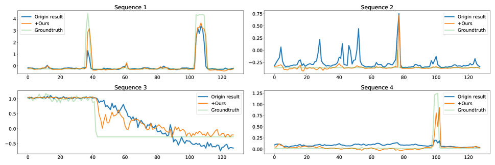
Figure 5: Prediction results on UK-Daleh1: We used four prediction sequences to demonstrate the enhanced load forecasting capability of our method under both changing and unchanging appliance operational states.

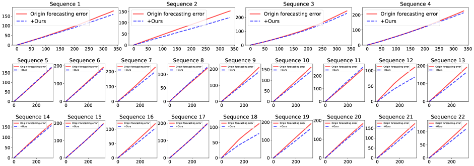
Figure 6: Prediction error results on the UMass House D: We visualized the prediction results for all 22 sequences of House D. In these visualizations, lower values indicate smaller errors compared to the actual values. It is evident that after using our method, the prediction errors of the model mostly decreased, with a few remaining stable. Additionally, as the prediction steps increase, the reduction in prediction error becomes more significant.

V-F Ablation Studies

Further, we perform ablative analysis to explore the effects of different components on the performance of our proposed ERKG. Specifically, ablation studies are conducted to investigate the effects of the different state predictor and the knowledge guide strategy, respectively.

Effect of State Predictor: Two state predictors are experimented: one using the proposed method with $D$ UEs (+ours), and the other using a state predictor that shares middle layer weights (w/o MSP). The first group of experiments aims to evaluate the efficiency of the proposed MSP in different datasets. We implement the proposed method by ETSformer (Origin), with the prediction length in $[1,6,12,24,36,48,60,72,168,336]$, where average performances are shown in Table IV. The results demonstrate that the proposed MSP outperforms the original prediction methods and another state predictor in all comparison results. This confirms the effectiveness of the proposed MSP approach, which involves independently learning the patterns of different load series before understanding the relationships between them. In Table V, the second group of experiments is designed to evaluate the efficiency of the proposed MSP in different prediction lengths with the same experiment settings. The experimental results indicate that compared to existing prediction methods and other state predictors, the proposed MSP achieved the best results in all comparison metrics.

TABLE IV: Ablation without MSP: the average metric which prediction length in $[1,6,12,24,36,48,60,72,168,336]$.

Method	Origin		w/o MSP		+ours
Metric	MAE	MAPE′	MAE	MAPE′	MAE	MAPE′
Ampds2	0.491	1.005	0.495	0.999	0.452	0.883
UK-Daleh1	0.576	1.101	0.574	1.089	0.535	1.050
UMassC	0.594	1.193	0.584	1.177	0.518	1.060
UMassD	0.471	0.866	0.453	0.850	0.436	0.810

TABLE V: ABLATION WITHOUT MSP: We conduct it on Ampds2 with HORIZON $[1,6,12,24,36,48,60,72,168,336]$.

Method	Origin		w/o MSP		+ours
Metric	MAE	MAPE′	MAE	MAPE′	MAE	MAPE′
1	0.440	0.884	0.452	0.906	0.415	0.826
6	0.479	0.992	0.490	0.984	0.445	0.881
12	0.494	1.015	0.495	1.011	0.448	0.888
24	0.490	1.019	0.496	1.004	0.452	0.894
36	0.496	1.009	0.497	1.017	0.454	0.890
48	0.497	1.021	0.498	1.014	0.455	0.890
60	0.495	1.018	0.499	1.018	0.451	0.869
72	0.500	1.021	0.500	1.010	0.456	0.893
168	0.506	1.024	0.508	1.006	0.465	0.888
336	0.514	1.049	0.516	1.023	0.477	0.905

TABLE VI: Ablation without Response Loss: the average metric which horizon in $[1,6,12,24,36,48,60,72,168,336]$.

Method	Origin		w/o Response Loss		+ours
Metric	MAE	MAPE′	MAE	MAPE′	MAE	MAPE′
Ampds2	0.491	1.005	0.516	1.045	0.452	0.883
UK-Daleh1	0.576	1.101	0.580	1.104	0.535	1.050
UmassC	0.594	1.193	0.600	1.196	0.518	1.060
UmassD	0.471	0.866	0.469	0.866	0.436	0.810

TABLE VII: ABLATION WITHOUT Response loss: We conduct it on Ampds2 with HORIZON $[1,6,12,24,36,48,60,72,168,336]$.

Method	Origin		w/o Response Loss		+ours
Metric	MAE	MAPE′	MAE	MAPE′	MAE	MAPE′
1	0.440	0.884	0.491	1.041	0.415	0.826
6	0.479	0.992	0.499	1.018	0.445	0.881
12	0.494	1.015	0.507	1.025	0.448	0.888
24	0.490	1.019	0.502	1.019	0.452	0.894
36	0.496	1.009	0.510	1.036	0.454	0.890
48	0.497	1.021	0.514	1.063	0.455	0.890
60	0.495	1.018	0.517	1.067	0.451	0.869
72	0.500	1.021	0.517	1.047	0.456	0.893
168	0.506	1.024	0.538	1.089	0.465	0.888
336	0.514	1.049	0.564	1.043	0.477	0.905

Effect of Knowledge Guide Strategy: Our proposed method utilizes a knowledge-guided mechanism based on event-response (+ours). Hence, we design the corresponding ablation study by comparing with a feature-based knowledge-guided approach (w/o Response Loss), which merges hidden feature maps with the model’s hidden feature maps for knowledge guidance [46]. The proposed method, implemented via ETSformer (Origin), is evaluated in two groups of experiments as shown in Table VI and VII. The first group assesses the efficiency of the proposed response-based knowledge transfer across different datasets, while the second group examines its efficiency across varying prediction lengths under the same experimental setup. The results show that the proposed method consistently outperforms in all comparison metrics, validating the effectiveness of the proposed knowledge-guided mechanism. Additionally, ablation experiments on the number of clusters for electrical appliances verify the effectiveness of the silhouette score to determine the optimal number of operational states, as detailed in Table VIII.

TABLE VIII: Ablation Study on the Number of Appliance Operational State Clusters ($K$)

Prediction Length	K=2	K=3	K=4	K=5	+ours
1	0.487	0.479	0.466	0.462	0.447
6	0.561	0.554	0.540	0.534	0.513
12	0.586	0.565	0.557	0.550	0.523
24	0.589	0.569	0.557	0.549	0.517
36	0.592	0.571	0.557	0.549	0.534
48	0.585	0.575	0.566	0.551	0.523
60	0.600	0.582	0.577	0.558	0.535
72	0.600	0.590	0.573	0.556	0.544
168	0.604	0.588	0.573	0.562	0.521
336	0.611	0.597	0.572	0.565	0.524

Comparison of Computational Cost: We perform ablation analysis to separately explore the additional time cost of applying our method and the training cost of our MSP. Accordingly, we conduct experiments on ETSformer: i) in Table IX, we compare the time per epoch ($t$, in seconds), the number of epochs ($N$) required to complete training, and the total training time ($T$, in seconds) before using our method (Origin) and after using our method (+ours). It can be seen that although our method increases the training time for a single epoch, in some cases, e.g., Ampds2, UK-Daleh1, UMassD, our method reduces the number of epochs needed for the model to converge, which can significantly reduce the overall training cost, sometimes even below the original time, e.g., Ampds2. ii) in Table X, we compare our Events Forecasting Model (MSP) with the original model (Origin). It is evident that the total training time of the MSP is less than that of the original prediction model in Ampds2, UK-Daleh1 and UMassC.

In existing datasets, a significant increase in data size may accelerate model convergence, resulting in training time not rising proportionally, as shown by Ampds2 in Table IX. There are two potential challenges for the implementation of ERKG in generic real-world setups. Firstly, although ERKG exhibits advantageous performance for individual households, it lacks generalizability across different residents, e.g., a model trained on one household may need retraining when applied to another due to variations in the quantity and types of appliances. Hence, applying ERKG across different households may increase training costs. Additionally, while ERKG effectively learns event-related associations among appliances, its computational cost rises correspondingly with higher data dimensions. In future works, it would be interesting to leverage knowledge distillation[31] to achieve light-weighting in modelling an optimization.

TABLE IX: COMPARISON OF TRAINING TIME BETWEEN OUR METHOD AND THE ORIGINAL METHOD.

Datasets	Ampds2	UK-Daleh1	UmassC	UmassD
Origin	577.49	757.43	122.24	165.81
($T=N*t$)	(48$*$12.03)	(65$*$11.65)	(23$*$5.31)	(27$*$6.14)
+ours	431.80	886.27	334.71	175.89
($T=N*t$)	(28$*$15.42)	(56$*$15.82)	(48$*$6.97)	(18$*$9.77)

TABLE X: TRAINING TIME COMPARISON BETWEEN EVENTS FORECASTING AND ORIGINAL METHODS.

Datasets	Ampds2	UK-Daleh1	UmassC	UmassD
Origin	577.49	757.43	122.24	165.81
($T=N*t$)	(48$*$12.03)	(65$*$11.65)	(23$*$5.31)	(27$*$6.14)
MSP	198.640	419.012	119.59	232.07
($T=N*t$)	(12$*$16.55)	(14$*$29.93)	(19$*$6.29)	(12$*$19.34)

VI Conclusion

In this work, we propose ERKG, a knowledge guided approach to enhance RLF models for both household-level and application-level electricity usage predictions. In ERKG, it learns event-related sparse knowledge from dense load series by leveraging a novel forecasting model for estimating electricity usage events and a corresponding knowledge-guided mechanism based on event response. With sparse knowledge from event response, ERKG are more effective at learning electricity usage event than the existing multivariates time series forecasting modle. Notably, ERKG can serve as a plug-in block during the forecasting model training stage, allowing existing models to focus more on sparse event information but less on noise, thereby improving performances. Extensive numerical experiments demonstrate that ERKG effectively enhances the RLF performance of existing state-of-the-art models, with an average improvement of 9% in MAE. Future directions could include considering covariates that influence events, such as exploring unlabeled modeling of the relationships between events, and considering how to ensure that the model’s computational cost, and the number of parameters remains within an appropriate range as the data size increases.

References

- [1] A. Chrysopoulos and P. Mitkas, “Customized time-of-use pricing for small-scale consumers using multi-objective particle swarm optimization,” Advances in Building Energy Research, vol. 12, no. 1, pp. 25–47, 2018.
- [2] T. Morstyn, N. Farrell, S. J. Darby, and M. D. McCulloch, “Using peer-to-peer energy-trading platforms to incentivize prosumers to form federated power plants,” Nature Energy, vol. 3, no. 2, pp. 94–101, 2018.
- [3] Y. Wang, Q. Chen, T. Hong, and C. Kang, “Review of smart meter data analytics: Applications, methodologies, and challenges,” IEEE Transactions on Smart Grid, vol. 10, no. 3, pp. 3125–3148, 2018.
- [4] S. Wang, X. Deng, H. Chen, Q. Shi, and D. Xu, “A bottom-up short-term residential load forecasting approach based on appliance characteristic analysis and multi-task learning,” Electric Power Systems Research, vol. 196, p. 107233, 2021.
- [5] W. Kong, Z. Y. Dong, Y. Jia, D. J. Hill, Y. Xu, and Y. Zhang, “Short-term residential load forecasting based on lstm recurrent neural network,” IEEE Transactions on Smart Grid, vol. 10, no. 1, pp. 841–851, 2017.
- [6] W. Kong, Z. Y. Dong, D. J. Hill, F. Luo, and Y. Xu, “Short-term residential load forecasting based on resident behaviour learning,” IEEE Transactions on Power Systems, vol. 33, no. 1, pp. 1087–1088, 2017.
- [7] W. Lin, D. Wu, and B. Boulet, “Spatial-temporal residential short-term load forecasting via graph neural networks,” IEEE Transactions on Smart Grid, vol. 12, no. 6, pp. 5373–5384, 2021.
- [8] H. Zhao, Y. Wu, L. Ma, and S. Pan, “Spatial and temporal attention-enabled transformer network for multivariate short-term residential load forecasting,” IEEE Transactions on Instrumentation and Measurement, vol. 72, no. 1, pp. 1–11, 2023.
- [9] M. Razghandi and D. Turgut, “Residential appliance-level load forecasting with deep learning,” in Proceedings of the 2020 IEEE Global Communications Conference (GLOBECOM), 2020, pp. 1–6.
- [10] Y. Zhou, A. S. Nair, D. Ganger, A. Tripathi, C. Baone, and H. Zhu, “Appliance level short-term load forecasting via recurrent neural network,” in Proceedings of the 2022 IEEE Power & Energy Society General Meeting (PESGM). IEEE, 2022, pp. 1–5.
- [11] S. S. Rangapuram, L. D. Werner, K. Benidis, P. Mercado, J. Gasthaus, and T. Januschowski, “End-to-end learning of coherent probabilistic forecasts for hierarchical time series,” in Proceedings of the 38th International Conference on Machine Learning (ICML), vol. 139. PMLR, 18–24 Jul 2021, pp. 8832–8843.
- [12] H. Zhou, S. Zhang, J. Peng, S. Zhang, J. Li, H. Xiong, and W. Zhang, “Informer: Beyond efficient transformer for long sequence time-series forecasting,” in Proceedings of the 35th AAAI Conference on Artificial Intelligence (AAAI), vol. 35, no. 12, 2021, pp. 11 106–11 115.
- [13] H. Wu, J. Xu, J. Wang, and M. Long, “Autoformer: Decomposition transformers with auto-correlation for long-term series forecasting,” in Proceedings of the 34th Advances in Neural Information Processing Systems (NIPS), vol. 34, 2021, pp. 22 419–22 430.
- [14] G. Woo, C. Liu, D. Sahoo, A. Kumar, and S. Hoi, “ETSformer: Exponential smoothing transformers for time-series forecasting,” arXiv preprint arXiv:2202.01381, 2022.
- [15] Y. Zhang and J. Yan, “Crossformer: Transformer utilizing cross-dimension dependency for multivariate time series forecasting,” in Proceedings of the 11th International Conference on Learning Representations (ICLR), 2022. [Online]. Available: https://openreview.net/forum?id=vSVLM2j9eie
- [16] A. Zeng, M. Chen, L. Zhang, and Q. Xu, “Are transformers effective for time series forecasting?” in Proceedings of the 37th AAAI Conference on Artificial Intelligence (AAAI), vol. 37, no. 9, 2023, pp. 11 121–11 128.
- [17] S.-A. Chen, C.-L. Li, S. O. Arik, N. C. Yoder, and T. Pfister, “TSMixer: An all-mlp architecture for time series forecast-ing,” Transactions on Machine Learning Research, 2023. [Online]. Available: https://openreview.net/forum?id=wbpxTuXgm0
- [18] V. Ekambaram, A. Jati, N. Nguyen, P. Sinthong, and J. Kalagnanam, “Tsmixer: Lightweight mlp-mixer model for multivariate time series forecasting,” in Proceedings of the 29th ACM SIGKDD Conference on Knowledge Discovery and Data Mining (KDD), 2023, p. 459–469.
- [19] M. Cho, J. Hwang, and C. Chen, “Customer short term load forecasting by using arima transfer function model,” in Proceedings of the 1995 International Conference on Energy Management and Power Delivery (EMPD), vol. 1, 1995, pp. 317–322 vol.1.
- [20] G. Xie, X. Chen, and Y. Weng, “An integrated gaussian process modeling framework for residential load prediction,” IEEE Transactions on Power Systems, vol. 33, no. 6, pp. 7238–7248, 2018.
- [21] R. K. Jain, K. M. Smith, P. J. Culligan, and J. E. Taylor, “Forecasting energy consumption of multi-family residential buildings using support vector regression: Investigating the impact of temporal and spatial monitoring granularity on performance accuracy,” Applied Energy, vol. 123, pp. 168–178, 2014.
- [22] B. Jiang, Y. Liu, H. Geng, Y. Wang, H. Zeng, and J. Ding, “A holistic feature selection method for enhanced short-term load forecasting of power system,” IEEE Transactions on Instrumentation and Measurement, vol. 72, no. 1, pp. 1–11, 2023.
- [23] S. Welikala, C. Dinesh, M. P. B. Ekanayake, R. I. Godaliyadda, and J. Ekanayake, “Incorporating appliance usage patterns for non-intrusive load monitoring and load forecasting,” IEEE Transactions on Smart Grid, vol. 10, no. 1, pp. 448–461, 2017.
- [24] B. Qian, Y. Zhu, Y. Xiao, Y. Zhang, X. Xu, and M. Zhou, “Variable input structure user load forecasting method based on user load state identification,” in Proceedings of the 2020 IEEE Sustainable Power and Energy Conference (iSPEC). IEEE, 2020, pp. 2583–2589.
- [25] X. Qi, K. Hou, T. Liu, Z. Yu, S. Hu, and W. Ou, “From known to unknown: Knowledge-guided transformer for time-series sales forecasting in alibaba,” arXiv preprint arXiv:2109.08381, 2021.
- [26] C. Yin, R. Zhao, B. Qian, X. Lv, and P. Zhang, “Domain knowledge guided deep learning with electronic health records,” in Proceedings of the 2019 IEEE International Conference on Data Mining (ICDM). IEEE, 2019, pp. 738–747.
- [27] H. Peng, N. Klepp, M. Toutiaee, I. B. Arpinar, and J. A. Miller, “Knowledge and situation-aware vehicle traffic forecasting,” in Proceedings of the 11th IEEE International Conference on Big Data (Big Data). IEEE, 2019, pp. 3803–3812.
- [28] F. Liu, C. Zeng, L. Zhang, Y. Zhou, Q. Mu, Y. Zhang, L. Zhang, and C. Zhu, “Fedtadbench: Federated time-series anomaly detection benchmark,” in Proceedings of the 24th IEEE International Conference on High Performance Computing & Communications (HPCC). IEEE, 2022, pp. 303–310.
- [29] Z. Zeng, W. Zhao, P. Qian, Y. Zhou, Z. Zhao, C. Chen, and C. Guan, “Robust traffic prediction from spatial–temporal data based on conditional distribution learning,” IEEE Transactions on Cybernetics, vol. 52, no. 12, pp. 13 458–13 471, 2022.
- [30] P. Wang, Y. Fan, L. Xia, W. X. Zhao, S. Niu, and J. Huang, “Kerl: A knowledge-guided reinforcement learning model for sequential recommendation,” in Proceedings of the 43rd International ACM SIGIR Conference on Research and Development in Information Retrieval (IR), 2020, pp. 209–218.
- [31] G. Hinton, O. Vinyals, and J. Dean, “Distilling the knowledge in a neural network,” arXiv preprint arXiv:1503.02531, 2015.
- [32] C. Yang, J. Pan, X. Gao, T. Jiang, D. Liu, and G. Chen, “Cross-task knowledge distillation in multi-task recommendation,” in Proceedings of the 36th AAAI Conference on Artificial Intelligence (AAAI), vol. 36, no. 4, 2022, pp. 4318–4326.
- [33] A. Langevin, M. Cheriet, and G. Gagnon, “Efficient deep generative model for short-term household load forecasting using non-intrusive load monitoring,” Sustainable Energy, Grids and Networks, vol. 34, p. 101006, 2023.
- [34] S. Haben, J. Ward, D. Vukadinovic Greetham, C. Singleton, and P. Grindrod, “A new error measure for forecasts of household-level, high resolution electrical energy consumption,” International Journal of Forecasting, vol. 30, no. 2, pp. 246–256, 2014.
- [35] Z. Xia, R. Zhang, H. Ma, and T. K. Saha, “Day-ahead electricity consumption prediction of individual household–capturing peak consumption pattern,” IEEE Transactions on Smart Grid, vol. 15, no. 3, pp. 2971–2984, 2024.
- [36] J. Dong, L. Luo, Y. Lu, and Q. Zhang, “A parallel short-term power load forecasting method considering high-level elastic loads,” IEEE Transactions on Instrumentation and Measurement, vol. 72, no. 1, pp. 1–10, 2023.
- [37] R. Tavenard, J. Faouzi, G. Vandewiele, F. Divo, G. Androz, C. Holtz, M. Payne, R. Yurchak, M. Rußwurm, K. Kolar, and E. Woods, “Tslearn, a machine learning toolkit for time series data,” Journal of Machine Learning Research, vol. 21, no. 118, pp. 1–6, 2020.
- [38] Y. Liu, Y. Zhou, K. Yang, and X. Wang, “Unsupervised deep learning for iot time series,” IEEE Internet of Things Journal, vol. 10, no. 16, pp. 14 285–14 306, 2023.
- [39] P. Ducange, F. Marcelloni, and M. Antonelli, “A novel approach based on finite-state machines with fuzzy transitions for nonintrusive home appliance monitoring,” IEEE Transactions on Industrial Informatics, vol. 10, no. 2, pp. 1185–1197, 2014.
- [40] L. Yu, H. Li, X. Feng, and J. Duan, “Nonintrusive appliance load monitoring for smart homes: Recent advances and future issues,” IEEE Instrumentation & Measurement Magazine, vol. 19, no. 3, pp. 56–62, 2016.
- [41] P. J. Rousseeuw, “Silhouettes: a graphical aid to the interpretation and validation of cluster analysis,” Journal of Computational and Applied Mathematics, vol. 20, pp. 53–65, 1987.
- [42] S. Makonin, B. Ellert, I. V. Bajić, and F. Popowich, “Electricity, water, and natural gas consumption of a residential house in canada from 2012 to 2014,” Scientific Data, vol. 3, no. 1, pp. 1–12, 2016.
- [43] J. Kelly and W. Knottenbelt, “The uk-dale dataset, domestic appliance-level electricity demand and whole-house demand from five uk homes,” Scientific Data, vol. 2, no. 1, pp. 1–14, 2015.
- [44] S. Barker, A. Mishra, D. Irwin, E. Cecchet, P. Shenoy, J. Albrecht et al., “Smart*: An open data set and tools for enabling research in sustainable homes,” in Proceedings of the 2012 Workshop on Data Mining Applications in Sustainability (SustKDD), 2012.
- [45] P. Goodwin and R. Lawton, “On the asymmetry of the symmetric mape,” International Journal of Forecasting, vol. 15, no. 4, pp. 405–408, 1999.
- [46] J. Xiao, D. Zhan, H. Qi, and Z. Jin, “When face completion meets irregular holes: An attributes guided deep inpainting network,” in Proceedings of the 29th ACM International Conference on Multimedia (MM), 2021, pp. 3202–3210.