Fast Mølmer-Sørensen gates in trapped-ion quantum processors with compensated carrier transition
Abstract
Carrier transition is one of the major factors hindering the high-speed implementation of Mølmer-Sørensen gates in trapped-ion quantum processors. We present an approach to design laser pulse shapes for Mølmer-Sørensen gate in ion chains which accounts for the effect of carrier transition on qubit-phonon dynamics. We show that the fast-oscillating carrier term effectively modifies the spin-dependent forces acting on ions, and this can be compensated by a simple nonlinear transformation of a laser pulse. Using numerical simulations for short ion chains and perturbation theory for longer chains, we demonstrate that our approach allows to reach the infidelity below while keeping the gate duration below .
I Introduction
High-fidelity entangling gates are critical for the practical realization of quantum computers. With cold trapped ions, remarkable progress in gate implementation has been achieved in recent decades [1]. Since Cirac-Zoller gate [2], various gate designs have been proposed and implemented, including Mølmer-Sørensen gate [3], light-shift gate [4], ultrafast gates [5], etc. Among them, Mølmer-Sørensen gate and its variations are the most ubiquitous.
Mølmer-Sørensen gate (MS gate) is implemented with the help of a bichromatic external field pulse, typically an optical or Raman laser beam, detuned symmetrically from the qubit transition [3]. In Lamb-Dicke regime, the field creates a spin-dependent force acting on ions, and the pulse parameters should be chosen to make ion trajectories closed curves in phase space. As a result, qubits acquire a spin-dependent phase and become entangled.
For a two-ion crystal, high-fidelity MS gates can be implemented with constant-amplitude field smoothly turned on and off [6]. For larger ion number, more complicated pulse shapes are required in order to close phase space trajectories for multiple motional modes of an ion crystal [7]. For amplitude-modulated pulses, the pulse shape is determined by a set of linear equations [7] which can be efficiently solved numerically.
In recent literature, a variety of pulse shaping approaches have been proposed for different purposes. Apart from amplitude modulation proposed in [7], phase modulation [8] and multi-tone beams [9] can be used. Also, additional constraints on the pulse shape allow to implemement parallel gates [10, 13], to enhance gate robustness against fluctuations of the experimental parameters [11, 12], or to minimize the total external field power [11].
To design laser pulses implementing MS gate with highest possible fidelity, a careful error analysis is necessary. The errors originate both from technical noises, such as laser and magnetic field fluctuations, and the intrinsic laser-ion interactions [14]. To account for the latter, it is necessary to go beyond the usual simplifying assumptions such as Lamb-Dicke and rotating-wave approximations often used to describe laser-ion dynamics. The latter can be achieved by a numerical simulation in the full ion-phonon Hilbert space or by applying a systematical procedure such as Magnus expansion beyond the leading order [15, 16].
One of the unwanted interactions present in trapped ions is the carrier transition. It is present when a bichromatic beam with two co-propagating plane wave components acts on ion qubits. Although for the MS gate operation the beam components should be close to qubit motional sidebands, direct qubit transition is also inevitably present. Its influence grows with increasing gate speed [6], and it becomes one of the dominant factors limiting gate fidelity at short gate times [14].
The theoretical analysis of ion dynamics with full account for carrier term has been performed for two ions interacting with a single phonon mode [17, 6]. it has been shown that the fast-oscillating carrier term results in a nonlinear renormalization of the driving field amplitude, and (for strictly rectangular pulse) in a basis rotation of the gate operator depending on the relative phase between the bichromatic beam components. For gate implementation in long chains, multiple phonon modes should be considered, and amplitude pulse shaping should ensure closed phase-space motional trajectories.
In this work, we present a theoretical analysis of the influence of carrier transition on MS gate dynamics in a multi-ion chain with account for all phonon modes. For amplitude-shaped pulse, we eliminate the carrier term in the system Hamiltonian by going into interaction picture. The leading part of the resulting Hamiltonian has the form of a spin-dependent force Hamiltonian, where carrier transition modifies the force values obtained from Lamb-Dicke expansion. We propose a family of pulse shapes which takes into account this modification. Our pulses can be found by applying a simple nonlinear transformation to a pulse obtained from linear equations. Using numerical simulations for short chains and perturbation theory calculations for longer chains, we demonstrate that our pulse-shaping scheme shows a considerable fidelity gain in comparison to pulses obtained from linear equations for gate times - microseconds and - ions, and the theoretical infidelity for our pulses is below .
So, our pulse-shaping approach provides a considerable speedup while maintaining high gate fidelity, which is a step towards meeting the challenging requirements for practical quantum computations.
II Dynamics of trapped ions qubits in the presence of carrier transition
We consider the trapped-ion quantum processor consistsing of a system of ions confined in a radio frequency Paul trap, where two electronic levels of each ion constitute qubit levels. We assume that ions form a linear crystal, therefore, ions share independent sets of collective phonon modes for each trap axis directions [18]. We consider the implementation of an entangling gate between two ion qubits with an amplitude-modulated bichromatic laser field symmetrically detuned from qubit transition. The interaction-picture Hamiltonian for the considered pair of ions reads [19]
| (1) |
where are the components of the laser field wavevector, are the components of ions displacememnts from their equilibrium positions, , and are the creation and annihilation operators of the phonon modes, are the phonon mode frequencies, are the Lamb-Dicke parameters, and is the bichromatic beam amplitude envelope. For the implementation of the target entangling gate, which we specify as the gate, one should find a pulse that the system evolution operator reduces to the target gate operator.
To find the approximate evolution operator, one can expand the system Hamiltonian in the Lamb-Dicke parameters. Up to the first order, the Hamiltonian reads
| (2) |
where
| (3) |
| (4) |
The Hamiltonian in Lamb-Dicke approximation contains two contributions and . The term is a spin-dependent force Hamiltoninan [20, 21]. The term corresponds to direct carrier transitions. Often, the contribution of is neglected. This approximation is valid when is close to one or several phonon mode frequencies, so contains slowly-oscillating terms which contribute the dynamics significantly, whereas is fastly oscillating.
For the implementation of an gate, an appropriate pulse shape should be found. Let be applied in the time interval . By comparing the target operator with the evolution operator (5), one gets the following conditions for and [21, 7]:
| (9) |
| (10) |
The equations (9) comprise linear equations for . The equations (9) can be solved by numerically by standard linear algebra routines. With approximations made, the resulting implements the MS gate with 100% fidelity.
However, even in the absence of technical noises, the neglected term contibutes to gate infidelity, and its importance grows with increasing gate speed. To account for the carrier term systematically, let us go into interaction picture with respect to :
| (11) |
where
| (12) |
After this transformation the Hamiltonian takes form
| (13) |
The transformation (11) is equivalent to the single-qubit rotations applied after the gate operation. These rotations could be compensated by applying additional resonant pulses after the gate operation. However, this is not necessary because the rotation angle can be greatly reduced by appropriate pulse design. In the following, we assume that satisfies the following conditions:
-
1.
varies slowly in comparison to ,
-
2.
and its first derivatives vanish in the beginning and in the end of the pulse.
Under these conditions and with our proposed pulse design (described in more detail in subsequent sections), we get typical values of of order -. Therefore, we can assume that the final state of the qubit-phonon system is determined only by evolution with the Hamiltonian (13).
To analyze the Hamiltonian (13), we suggest to split it into two parts, the leading order part and the perturbation part , as shown by underbraces. The perturbation alone reads
| (14) |
Such a decomposition is justified under two assumptions on :
-
1.
oscillates near zero;
-
2.
its magnitude remains .
These assumptions hold for all the pulses that will be considered below. With these assumptions, the term oscillates near and gives a contribution important on large time scales. In contrast, oscillates near zero, so its contribution cancels on large time scales. Because of that, it is reasonable to consider the sine term as a perturbation.
The leading-order term has the form of a spin-dependent forces Hamiltonian, so its propagator has the same form as (5):
| (15) |
where
| (16) |
| (17) |
| (18) |
Because of the transformation into the interaction picture generated by the carrier term, the spin-dependent forces get an additional term.
In addition, the evolution operator is modified by perturbative corrections generated by . Within the first-order perturbation theory by , the evolution operator of the Hamiltonian (13) can be expressed as
| (19) |
where
| (20) |
As the perturbation contains the sigma matrices , the operator causes the spin flip processes in -basis: for the initial qubit state (Pauli string in -basis), it causes transitions to another Pauli string which differs from the initial state by a single spin flip. However, in the next sections, we show that these processes cause only a small correction to the system evolution for the considered pulses. Therefore, we can use the expression (15) for the description of gate dynamics and for the determination of the pulse shape .
With modified expressions for spin-dependent forces, we get new conditions for the implementation of :
| (21) |
III Contributions of carrier term to gate infidelity
The expressions (15) and (19) for the propagator can be used for analytical calculation of the gate fidelity of an ion chain of arbitrary length. In this section, we present the expressions for the gate fidelity defined in the full ion-phonon Hilbert space. We assume that the ion chain is cooled to the ground state at the beginning of the gate operation, so the initial state of the qubit-phonon system is , where is the initial qubit state. The action of the ideal gate turns qubits into the state but leaves all phonon modes in the ground state. Therefore, we can characterize the gate realization by fidelity between the state (the outcome of the ideal gate) and the state obtained after the evolution with the Hamiltonian (1):
| (22) |
Due to imperfect pulse design, and may deviate from target values of Eq. (21) in the end of the gate. Because of that, already the leading-order term of the evolution operator will not coincide with the ideal operator. So, it is meaningful to define another fidelity measure (zero-order fidelity) obtained from the leading-order propagator :
| (23) |
In Appendix B, we find for various initial states . In particular, for (Pauli strings in the -basis, ), the infidelity reads
| (24) |
where . We see that incomplete closure of the phase trajectories and the error in the angle give two additive contributions into the average gate infidelity. Our expressions slighlty differ from [14], [21] due to our different fidelity definition.
Also, for (Pauli strings in -basis), zero-order gate infidelity is given by expression
| (25) |
In this case, the error in does not contribute to gate fidelity. At small , the infidelity can be interpreted as the probability of phonon excitation after the gate operation.
Then, let us find the contribution to infidelity caused by the spin-flip perturbation accounted by the term in the evolution operator (19). For simplicity, we consider only the initial states . The spin flip probability for such initial states is
| (26) |
In Appendices B and C, we derive the explicit expression (63) for as a two-dimensional integral over time. The integral (63) is suitable for the calculation of the spin flip probability for long ion chains where the full numerical solution is not feasible.
Also, we show that the gate infidelity for the initial states with account for the carrier transition reads
| (27) |
so the contributions of imperfectly closed phase trajectories and spin flip error are additive. For other qubit states, there are interference terms between the two considered contributions into error.
Finally, we show that the infidelity averaged over all initial qubit states over the Fubini-Study measure:
| (28) |
where given by Eq. (23) accounts only for the leading-order term of . Therefore, it is sufficient to calculate the contribution of only for the initial states to find an upper bound for the average gate infidelity.
Thus, carrier term contributes into two types of gate error. First, it modifies the values of the spin-dependent forces, so it causes incomplete closing of the phase trajectories unless the pulse shape is chosen appropriately. Second, it causes the spin-flip error arising from . In the following, we present a method to find pulses which approximately close the phase trajectories with account for the modification of the spin-dependent forces by carrier term.
IV Pulse shaping scheme
In this section, we present a method to find pulse shapes which approximately satisfy the Eqs. (21). Then, we demonstrate its performance on a particular example of a 5-ion chain and compare the pulse obtained by our method with the pulse obtained from linear Eqs. (9), (10). We show that it strongly reduces the contribution of and to the zero-order infidelity , thus increasing the overall fidelity.
Assume that satisfies the smoothness conditions from Section II, so it varies slowly on the timescale and is smoothly turned on (off) at the beginning (end) of the gate. Then, the term in Eq. (18) can be approximately averaged over fast oscillations on the timescale . In Appendix D, we demonstrate that averaging allows to replace in Eq. (18) with
| (29) |
where
| (30) |
and are Bessel functions. As a result, the term in Eqs.(16), (17) causing the nonlinearity of Eqs. (21) disappears. Thus, and can be calculated with Eqs. (6), (7) as there were no carrier term, but with replaced by .
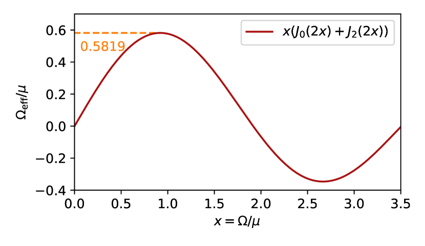
The transformation given by Eq. (30) can be thought as a nonlinear squeezing transformation of . In Fig. 1), we depict the functional dependence of on . When , . At larger , grows slower than until it reaches its absolute maximum , where . At even larger , has an oscillatory dependence on . This behavior of shows that the presence of the carrier term effectively reduces the field amplitude acting on an ion qubit.
| Num. (LD) | ||
|---|---|---|
| Num. (full) |
| Eq. (27) | Num. (LD) | Num. (full) | Eq. (27) | Num. (LD) | Num. (full) | ||
|---|---|---|---|---|---|---|---|
With knowledge of the transformation (30), we can find approximate solutions of the nonlinear equations (21) in two simple steps:
- 1.
- 2.
The pulse obtained after the step 1 would implement the gate if the carrier term was not present. By the step 2, is transformed to account for the modified expressions for the spin-dependent forces.
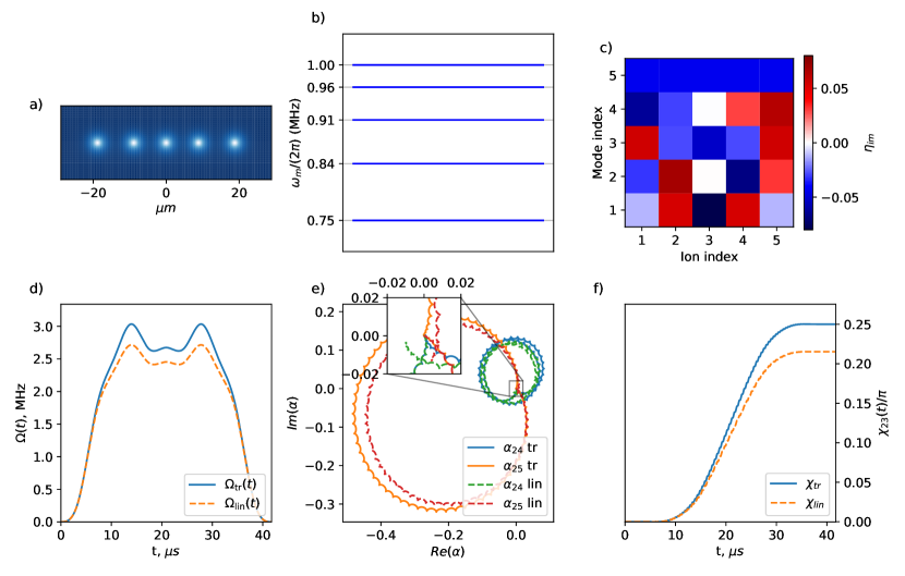
Let us illustrate the presented pulse shaping scheme on a particular example. We consider a chain of ions in a harmonic pseudopotential with radial frequency of MHz and the axial frequency of . The frequency of the lowest radial mode at these parameters is . We calculate the ion equilibrium positions, phonon normal modes and frequencies and Lamb-Dicke parameters of the chain using standard methods [18] (see Fig.2a-c). Then, we find the pulses implementing the gate between the second and the third ions of the chain for the gate time s, the detuning , and the motional phase .
First, we find a solution of Eqs. (9), (10). satisfying the smoothness conditions of the Section II. We split the interval into equal segments and search for as a piecewise-cubic polynomial (cubic spline). We require continuity up to the first-order derivatives and vanishing values and derivatives at the beginning and at the end of the gate. Under these requirements, Eqs. (9), (10) have a unique solution (see Appendix A). Then, we apply the inverse transformation (30) to find . For the considered 5-ion chain, and are shown in Fig. 2c.
For both pulses ( and ) we consider the system dynamics during the gate. Using Eqs. (16), (17), we find and entering the propagator (15). For the center-of-mass (COM) and stretch modes of an ion crystal, the phase trajectories are shown in Fig. 2e, and the time dependence of is shown in Fig. 2f. From Fig. 2e, it is clear that the phonon mode trajectories are not perfectly closed for the pulse . In contrast, for they are almost perfectly closed. Also, the value of at the end of the gate for significantly deviates from the target value of , whereas the deviation is much smaller for .
The calculated values of and at the end of the gate allow to predict the gate infidelity without the spin-flip contribution using Eq. (24). For the initial state, the results are presented in Table 1. One can see that the theoretical infidelity for the pulse is , which is in agreement with almost perfect phase trajectory closing shown in Fig. 2e and the correct value of . In contrast, the predicted infidelity for the pulse is of order .
To verify these predictions, we solve numerically the time-dependent Schrodedinger equation (TDSE) for the Hamiltonian (1) using QuTiP [22]. The calculated infidelities for both pulses are also in Table 1. For , the infidelity is slightly higher than the theoretical prediction, but also of order . For , the infidelity is approximately , which is more than two orders of magnitude lower than for . However, it is more than order of magnitude higher than the analytical value. We attribute this difference to the higher-order terms in the Lamb-Dicke parameters, which are not taken into account by our calculations but are present in the full Hamiltonian (1). To confirm this, we also solve TDSE for the Hamiltonian (2), where the higher-order terms of the expansion are neglected. The results, also presented in Table 1, show better agreement with the analytical predictions. The discrepancy in this case can be attributed to the higher orders of the perturbation theory in .
In addition, we analyze the gate fidelity for the initial states . In this case, Eq. (27) allows to separate the contributions of imperfectly closed phase trajectories and spin flips. Also, these contributions can be identified from numerical solution of TDSE: the first term in Eq. (27) equals the probability of phonon mode excitation, and the second term equals the probability of a spin flip. Both these probabilities can be extracted from the TDSE solution. In Table 2, we present the results of analytical calculations and TDSE solution with both types of Hamiltonians for the initial states .
The results confirm that the first-order perturbation theory in gives an accurate description of the dynamics with the first-order Hamiltonian (2). Indeed, for , the probabilities and calculated analytically and numerically are in good agreement. For , the spin flip probability is also accurately predicted by the analytical formula. The analytical formula for is less accurate, but it predicts correctly the very small magnitude of phonon excitation probability, .
For the simulation of the full Hamiltonian (1) with pulses , the considered contribution into error again match with the analytical predictions. However, for , both of the contributions are by order of magnitude larger than the corresponding analytical predicions. Still, the total error for is more than by order of magnitude lower than for .
From these results, we conclude that the dominant contributions into gate error for are indeed given by Eq. (24). These contributions, namely the error in the rotation angle and the imperfect closing of the phase trajectories, can be almost canceled by transforming into . The spin-flip contribution gives a negligibly small contribution into error for both pulses. Thus, the pulse allows the implementation of a fast high-fidelity gate in a 5-ion chain.
V Calculations
The results of the previous section can be used to implement a fast high-fidelity gate in a five-ion chain for a particular gate time and bichromatic detuning. Now let us examine the applicability of the method for other gate times, detunings, and chain lengths. Below, we find the parameter domains for which the method of Section IV can be implemented. For the 5-ion chain considered previously, we peform analytical and numerical calculations for different parameter values and study the fidelity dependence on these parameters. For longer ion chains which cannot be treated numerically, we perform only analytical calculations.
The transformation proposed in IV acts on pulses obtained with the usual pulse shaping approach with additional smoothness requirements. These pulses depend on the number of ions, the values of normal mode frequencies, the Lamb-Dicke parameters, the detuning of the bichromatic beam, the gate time and the additional requirements for the pulse shape. The normal mode frequencies and the Lamb-Dicke parameters depend on the trap frequencies, ion masses and the wavevectors, however, these dependencies are rather simple and do not contain fastly oscillating contributions. In contrast, the dependence on and is highly non-trivial because they enter the pulse shaping equations inside the oscillatory integrals (32). The dependence on the motional phase is weak providing that the field amplitude is smoothly turned on and off. Therefore, we mostly focus on the dependence on and .
A key point for the implementation of our scheme is the existence of the inverse transformation . As shown in previous section (see Eq. (30) and Fig. 1), the effective field amplitude has an absolute maximum of : therefore, is defined only in the range . So, for the step 2 of the pulse shaping procedure in Section IV, it is necessary that the absolute value of obtained from linear equations does not exceed . It is useful to find the set of parameters and for which this condition is satisfied. Below we call such sets on the plane allowed areas. As shown below, allowed areas have complicated shape due to the nontrivial dependence of on and .
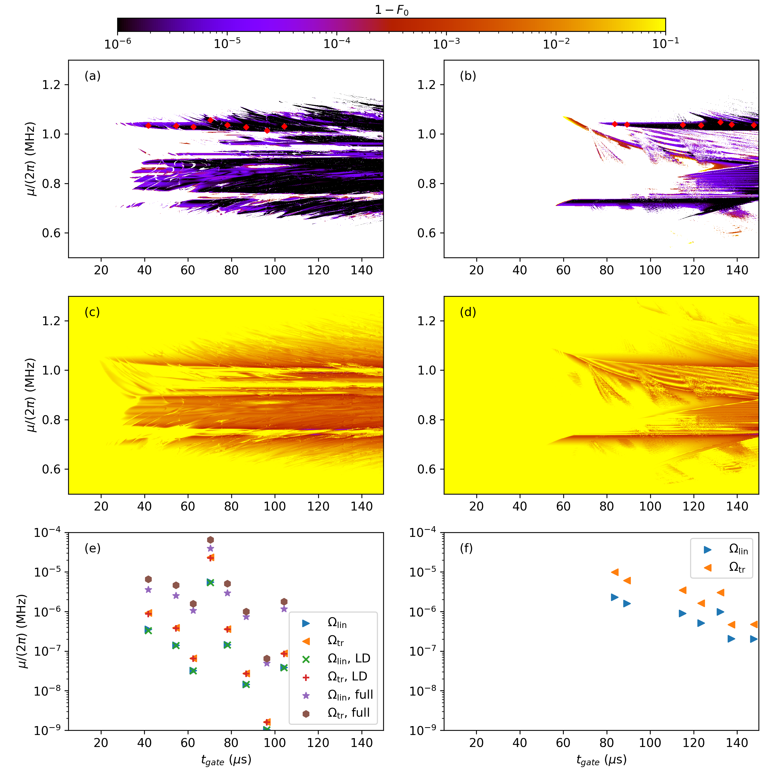
First, we find the allowed area for the 5-ion chain considered in the previous section. For that, we calculate for a sufficiently dense grid in - plane () for gate times from to s and detunings from to . The area is shown by color in Fig. 3a with its border indicated by a solid line. Along the vertical axis, the area occupies the values of lying closely to the band of radial phonon frequencies. Along the horizontal axis, it spans the whole range of except the values below .
For each point inside the allowed area, we also calculate the transformed pulse . Using Eq. (24), we calculate the leading-order contribution to gate infidelity for the initial state for each pair . The result is shown in Fig. 3a by color. We find that infidelity is of order nearly for all points inside the area except the vicinity of the boundaries.
For comparison, we calculate for pulses with the initial state in the entire grid. The result is shown in Fig 3(c). We find that the infidelity for is considerably larger than for inside the allowed area and it becomes even larger outside it.
We also perform these calculations for a 20-ion chain. All laser and trap parameters are taken the same as for 5-ion case except the axial frequency, which is set to , and the number of segments in the pulse, which is . With such value of axial frequency, radial phonon modes are all in the range as for the 5-ion case. In Fig. 3(b,d), we show the results for a 20-ion chain. Analogously with the 5-ion case, we find the allowed area and calculate for and in the plane. The 20-ion allowed area (see Fig. 3(b)) has a shape similar to the 5-ion case, however, it is shifted to larger gate times: the minimal time for points inside the area is . Analogously with the 5-ion case, we find that is of order for (see Fig. 3(b)) and of order for (see Fig. 3(d)).
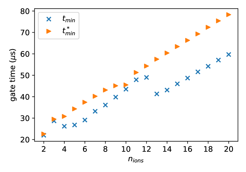
For other chain lengths from 2 to 20, we get analogous results. In Fig. 5, we show the dependence of the minimal time () inside the allowed area on the number of ions. Also, for each , we find the minimal gate time for which reaches (). Both of these times grow monotonically with the increasing number of ions, with exceeding no more than by .
Also, we calculate analytically the spin flip probability for a selected set of points in plane inside the area for 5-ion and 20-ion chains with the initial state . The points are shown in Fig. 3(a) (5 ions) and Fig. 3(b) (20 ions). The values of the spin flip probability are shown in Fig. 3(e) and Fig. 3(f). For all selected points, the spin flip probability for a 5-ion chain does not exceed , and it is even smaller for a 20-ion chain.
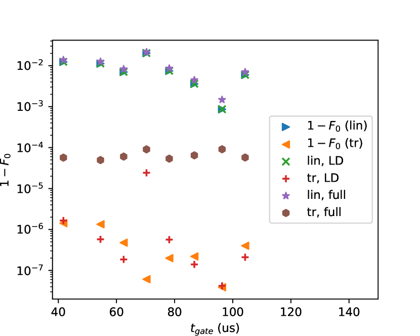
In addition, we perform numerical simulations for a selected set of points shown in Fig. 3(a) for a 5-ion chain. For each pair indicated by a point, we model gate dynamics by solving TDSE with the pulses and for the initial states and .
For the initial states , we calcucate the spin flip error as in Section IV: we compared the simulations with full Hamiltonian, with the Hamiltonian expanded up to the first order in Lamb-Dicke parameters, and the perturbation theory. The results of these simulations confirm the findings of the Section IV: perturbation theory gives an accurate result for the first-order Hamiltonian (2), but the spin flip probability is by order of magnitude higher for the full Hamiltonian (1). Even for the full Hamiltonian, is of order for most of the simulations.
For the initial states , we perform calculations similar to that Table 1. We compare the analytical zero-order infidelity given by Eq. (24) with the infidelity obtained from TDSE. The results are presented in Fig. 4. For all points, the infidelity for the pulses is considerably lower than for . By comparing the numerical indidelities for the full Hamiltonian and the Hamiltonian in the first order of the Lamb-Dicke expansion, we conclude that the Eq. (24) gives a leading-order contribution to the error for , and the dominant contribution to the the error for comes from the higher orders of the Lamb-Dicke expansion.
These results show that the conclusions of the section IV persist for a wide range of these parameters providing that and are within the allowed area. Also, the calculations prove that the zero-order error can be reliably used to estimate fidelity gain given by our scheme.
For gate times of tens of microseconds, our scheme allows to reduce the gate error from for non-optimized pulses to . Thus, our scheme facilitates the implementation of fast high-fidelity MS gates in chains with tens of ions, which is crucial for speeding up trapped-ion quantum computation.
VI Conclusions
We propose an amplitude-pulse-shaping method for the implementation of the Molmer-Sorensen entangling gate in linear chains of trapped-ion qubits. Our method allows to considerably reduce the error originating from carrier transition, which is always present in ions interaction with bichromatic external field. We show that a certain nonlinear transformation of the laser pulse allows to compensate the modification of the spin-dependent forces by carrier transition almost entirely, thus enabling a fast high-fidelity gate. For short ion chains, we show analytically and numerically that our method allows the fidelity gain is 2-3 orders of magnitude for gate times of - , with the resulting fidelity below . According to our analytical calculations, these conclusions persist for longer chains at least up to 20 ions.
Acknowledgements.
This work was supported by Rosatom in the framework of the Roadmap for Quantum computing (Contract No. 868-1.3- 15/15-2021).References
- Bruzewicz et al. [2019] C. D. Bruzewicz, J. Chiaverini, R. McConnell, and J. M. Sage, Trapped-ion quantum computing: Progress and challenges, Applied Physics Reviews 6, 021314 (2019).
- Cirac and Zoller [1995] J. I. Cirac and P. Zoller, Quantum computations with cold trapped ions, Physical Review Letters 74, 4091 (1995).
- Sørensen and Mølmer [2000] A. Sørensen and K. Mølmer, Entanglement and quantum computation with ions in thermal motion, Phys. Rev. A 62, 022311 (2000).
- Leibfried et al. [2003] D. Leibfried, B. DeMarco, V. Meyer, D. Lucas, M. Barrett, J. Britton, W. M. Itano, B. Jelenković, C. Langer, T. Rosenband, and D. J. Wineland, Experimental demonstration of a robust, high-fidelity geometric two ion-qubit phase gate, Nature 422, 412 (2003).
- Mizrahi et al. [2013] J. Mizrahi, B. Neyenhuis, K. Johnson, W. C. Campbell, C. Senko, D. Hayes, and C. Monroe, Quantum control of qubits and atomic motion using ultrafast laser pulses, Applied Physics B 10.1007/s00340-013-5717-6 (2013), arXiv:1307.0557 [physics.atom-ph] .
- Kirchmair et al. [2008] G. Kirchmair, J. Benhelm, F. Zähringer, R. Gerritsma, C. F. Roos, and R. Blatt, Deterministic entanglement of ions in thermal states of motion, New. J. Phys. 11, 023002 (2009) 10.1088/1367-2630/11/2/023002 (2008), arXiv:0810.0670 [quant-ph] .
- Choi et al. [2014] T. Choi, S. Debnath, T. Manning, C. Figgatt, Z.-X. Gong, L.-M. Duan, and C. Monroe, Optimal quantum control of multimode couplings between trapped ion qubits for scalable entanglement, Physical Review Letters 112, 190502 (2014).
- Milne et al. [2020] A. R. Milne, C. L. Edmunds, C. Hempel, F. Roy, S. Mavadia, and M. J. Biercuk, Phase-modulated entangling gates robust to static and time-varying errors, Physical Review Applied 13, 024022 (2020).
- Shapira et al. [2018] Y. Shapira, R. Shaniv, T. Manovitz, N. Akerman, and R. Ozeri, Robust entanglement gates for trapped-ion qubits, Physical Review Letters 121, 180502 (2018).
- Grzesiak et al. [2020] N. Grzesiak, R. Blümel, K. Wright, K. M. Beck, N. C. Pisenti, M. Li, V. Chaplin, J. M. Amini, S. Debnath, J.-S. Chen, and Y. Nam, Efficient arbitrary simultaneously entangling gates on a trapped-ion quantum computer, Nature Communications 11, 10.1038/s41467-020-16790-9 (2020).
- Blümel et al. [2021] R. Blümel, N. Grzesiak, N. Pisenti, K. Wright, and Y. Nam, Power-optimal, stabilized entangling gate between trapped-ion qubits, npj Quantum Information 7, 10.1038/s41534-021-00489-w (2021).
- Ruzic et al. [2024] B. P. Ruzic, M. N. Chow, A. D. Burch, D. S. Lobser, M. C. Revelle, J. M. Wilson, C. G. Yale, and S. M. Clark, Leveraging motional-mode balancing and simply parametrized waveforms to perform frequency-robust entangling gates, Physical Review Applied 22, 014007 (2024).
- Olsacher et al. [2020] T. Olsacher, L. Postler, P. Schindler, T. Monz, P. Zoller, and L. M. Sieberer, Scalable and parallel tweezer gates for quantum computing with long ion strings, PRX Quantum 1, 020316 (2020).
- Wu et al. [2018] Y. Wu, S.-T. Wang, and L.-M. Duan, Noise analysis for high-fidelity quantum entangling gates in an anharmonic linear paul trap, Phys. Rev. A 97, 062325 (2018).
- Vedaie et al. [2023] S. S. Vedaie, E. J. Páez, N. H. Nguyen, N. M. Linke, and B. C. Sanders, Bespoke pulse design for robust rapid two-qubit gates with trapped ions, Phys. Rev. Res. 5, 023098 (2023).
- Blümel et al. [2024] R. Blümel, A. Maksymov, and M. Li, Toward a mølmer sørensen gate with .9999 fidelity, Journal of Physics B: Atomic, Molecular and Optical Physics 57, 205501 (2024).
- Roos [2007] C. F. Roos, Ion trap quantum gates with amplitude-modulated laser beams, New Journal of Physics 10, 013002 (2008) 10.1088/1367-2630/10/1/013002 (2007), arXiv:0710.1204 [quant-ph] .
- James [1998] D. James, Quantum dynamics of cold trapped ions with application to quantum computation, Applied Physics B: Lasers and Optics 66, 181 (1998).
- Monroe et al. [2021] C. Monroe, W. Campbell, L.-M. Duan, Z.-X. Gong, A. Gorshkov, P. Hess, R. Islam, K. Kim, N. Linke, G. Pagano, P. Richerme, C. Senko, and N. Yao, Programmable quantum simulations of spin systems with trapped ions, Reviews of Modern Physics 93, 025001 (2021).
- Haljan et al. [2005] P. C. Haljan, K.-A. Brickman, L. Deslauriers, P. J. Lee, and C. Monroe, Spin-dependent forces on trapped ions for phase-stable quantum gates and entangled states of spin and motion, Physical Review Letters 94, 153602 (2005).
- Zhu et al. [2006] S.-L. Zhu, C. Monroe, and L.-M. Duan, Arbitrary-speed quantum gates within large ion crystals through minimum control of laser beams, Europhysics Letters (EPL) 73, 485 (2006).
- Johansson et al. [2013] J. Johansson, P. Nation, and F. Nori, Qutip 2: A python framework for the dynamics of open quantum systems, Computer Physics Communications 184, 1234 (2013).
- Nielsen and Chuang [2010] M. A. Nielsen and I. L. Chuang, Quantum Computation and Quantum Information (Cambridge University Press, 2010).
- Scully and Zubairy [1997] M. O. Scully and M. S. Zubairy, Quantum Optics (Cambridge University Press, 1997).
Appendix A Pulse shaping with piecewise-polynomial pulses
To implement the MS gate, one needs to find the pulse envelope which satisfies Eqs. (21). These equations comprise a system of linear and one quadratic equations on .
Assume that is decomposed into a basis set , , where the functions are defined on the interval of the gate duration. Then, the equations reduce to a linear system [14]
| (31) |
where
| (32) |
and the equation reduces to a quadratic equation
| (33) |
where
| (34) |
In order to ensure the smoothness conditions necessary for the consideration of Section IV, we search for in form of a cubic spline defined by its values in the points evenly spaced in the interval , , where . The basis functions are defined as cubic splines on the interval satisfying the boundary conditions , and the conditions , .
Appendix B MS gate fidelity with account for first-order spin-flip correction
In this Appendix, we derive expressions for the Molmer-Sorensen gate fidelity with account to three contributions: incompletely closed phonon mode phase trajectories, error in MS rotation angle, and spin-flip contribution. We consider fidelity in the full ion-phonon Hilbert space assuming that all phonon modes are initially cooled to the ground state. So, fidelity is defined as squared overlap between the target state and the resulting state:
| (35) |
To find using perturbation theory, it is convenient to denote the combination as
| (36) |
Using the unitarity of , we can rewrite fidelity in the form more suitable for perturbative calculation:
| (37) |
Then, we use the MS gate propagator with the first-order correction from the spin-flip perturbation (19). Let us give a small-error expansion of . We assume that and the deviation of from the target values are small, so the MS propagator can be decomposed as
| (38) |
where
| (39) |
After that, can be approximated as
| (40) |
where we define by Eq.(20), and neglect the term . We find convenient to separate the contributions of and into gate indfidelity. For that, we define two auxiliary fidelities. The first one is the fidelity of the state obtained by the action of the MS propagator (15),
| (41) |
It contains only the contributions of the imperfectly closed phase trajectories and the error in MS rotation angle. The second one is the fidelity between the states and :
| (42) |
It characterizes the deviation of the full evolution operator from the Molmer-Sorensen propagator (15) and is determined by . Similarly with (37), we can express and as
| (43) |
and
| (44) |
The auxiliary fidelities (41), (42) are helpful for analysing the fidelity (35). First, the fidelity (35) for any initial state can be bounded using the triangle inequality for fidelities [23]:
| (45) |
Then, let us prove that the infidelity (37) averaged over initial states is simply a sum of (43) and (44). Indeed, the average of (37) can be calculated as
| (46) |
where denotes the trace over qubit space. Then, we substitute the Eq. (40) into Eq. (46). As commutes with all , and contains only terms flipping the pseudospin direction along the axis, all cross-products of and vanish. Therefore, we get
| (47) |
Using Eq. (46), we get the following expression for :
| (48) |
The contribution averaged over initial states can be bounded from above as an average over all qubit basis states in the -basis, which simply follows from Eq. (46):
| (49) |
A closed-form representation of the term , which is the probability of a spin flip during the MS gate operation for the initial state , is given in Appendix C.
Now let us give expressions for some particular initial states. First of all, let us take the initial state of the form . Similarly with the average fidelity, the action of and in the qubit space implies that the infidelity is a sum of contributions from these operators. We get
| (50) |
| (51) |
| (52) |
Here does not contribute into error as it is responsible only for the phase between different qubit basis vectors in -basis.
Finally, let us give expressions for for the initial state (a spin string in -basis) and for an arbitrary superposition of qubit states in basis:
| (53) |
For ,
| (54) |
For a superposition with arbitrary coefficients ,
| (55) |
The expressions for for the latter states can be obtained in the same way. In general, they contain the interference terms coming from products of and .
Appendix C Spin flip probability
In this Appendix, we derive a closed-form representation of the probability of a spin flip during the MS gate operation for the initial state , which is given by the matrix element , We represent it as as a two-dimensional integral. From Eq. (20), we get
| (56) |
The propagator given by Eq. (15) is diagonal in qubit space and contains displacement operators in phonon space and can be represented as
| (57) |
where is the matrix , and
| (58) |
The perturbation can be written as
| (59) |
with
| (60) |
| (61) |
| (62) |
By substituting these expressions into Eq. (56) and taking the required matrix element, one gets
| (63) |
The matrix elements of the products of displacement operators and creation and annihilation operators can be calculated using the identites for displacement operators which can be found in quantum optics textbooks (see, for example, [24]). Below we give the expressions for the matrix elements for all combinations of , which corresponds to all combinations of creation and annihilation operators:
| (64) | ||||
Appendix D Derivation of the expression for effective
The integrals for and entering the MS propagator (Eqs. (16) and (17)) contain the term (Eq.(18)) which contains a fastly-oscillating term as a multiplier. Here we show how the fast oscillations can be approximately averaged to get rid of the nonlinear dependence on . For that, let us rewrite in the following way:
| (65) |
With underbraces, we show the parts which we consider as slowly (fastly) varying. We assume that the slow part does not change significantly over several periods of carrier oscillations . Then, we can average the fast part assuming that is approximately constant. Also, due to the assumptions on made in Section IV, we can replace by the leading-order asymptotic contribution:
| (66) |
After that, the fast part can be averaged as follows:
| (67) |
where are Bessel functions. For constant , this have been done in [17].