Strategic Investment to Mitigate Transition Risks

Abstract

This paper investigates strategic investments needed to mitigate transition risks, particularly focusing on sectors significantly impacted by the shift to a low-carbon economy. It emphasizes the importance of tailored sector-specific strategies and the role of government interventions, such as carbon taxes and subsidies, in shaping corporate behavior. In providing a multi-period framework, this paper evaluates the economic and operational trade-offs companies face under four various decarbonization scenarios—immediate, quick, slow, and no transitions. The analysis provides practical insights for both policymakers and business leaders, demonstrating how regulatory frameworks and strategic investments can be aligned to manage transition risks while optimizing long-term sustainability effectively. The findings contribute to a deeper understanding of the economic impacts of regulatory policies and offer a comprehensive framework to navigate the complexities of transitioning to a low-carbon economy.

Keywords: Transition Risk, Low-Carbon Economy, Government Intervention, Decarbonization Scenarios.

1 Introduction

1.1 Climate Risks

Mitigating climate change requires rapid and extensive decarbonization of the global economy. Climate change poses severe risks, such as altering extreme weather patterns and threatening ecosystems. Nonlinear climate dynamics can lead to sudden, irreversible changes, such as a polar ice melt or an ecosystem collapse, representing critical tipping points in Earth’s systems (Lenton et al. (2008)). The 2015 Paris Agreement underscores the urgency of limiting a global temperature rise to well below 2°C to prevent catastrophic outcomes, with net-zero carbon emissions needed by mid-century to meet this goal (Holden et al. (2018)).

Achieving decarbonization demands transformative changes across industries. While sectors like a power generation have made strides toward a renewable energy adoption, industries such as a steel and aviation lag due to underdeveloped low-carbon alternatives (Kober et al. (2020), Dietz et al. (2020)). These challenges highlight the importance of understanding climate risks, which fall into two categories: physical and transition risks. Physical risks encompass direct impacts of climate change, such as extreme weather events, while transition risks arise from shifting to a low-carbon economy driven by regulations, technologies, and societal demands (Carney (2015)). This paper prioritizes transition risks, as they offer more scope for a strategic intervention and remain underexplored in quantitative modeling (Cisagara (2024)).

1.2 Understanding Transition Risk

Transition risks result from structural changes in industries due to the shift toward a low-carbon economy. High-emission sectors, such as steel, aviation, and energy-intensive manufacturing, face challenges adapting to stricter regulations and cleaner technologies. Policy uncertainty adds complexity, creating financial risks for firms and investors (Holden et al. (2018)). These risks include stranded assets, increased credit risk, and volatility in asset returns (Semieniuk et al. (2021)).

While low-carbon policies, such as carbon taxes and emissions trading schemes, are essential for meeting climate objectives, their implementation introduces non-trivial transitional challenges (Bank of England (2018)). Companies are now evaluated not only on their financial metrics but also on their resilience to climate risks (Schulte and Hallstedt (2018)). Addressing these risks effectively requires targeted strategies and robust quantitative models.

1.3 Low-Carbon Transformation: Balancing Benefits and Challenges

The shift toward a low-carbon economy offers opportunities, such as cost savings, market leadership, and innovation, alongside significant challenges. Companies like Tesla and BP have successfully aligned with low-carbon strategies, reaping benefits such as new revenue streams and enhanced competitiveness. However, this effort of transition is capital-intensive, with high upfront costs and regulatory uncertainty posing risks to companies (NGFS (2019), Schulte and Hallstedt (2018)). Additionally, the rapid pace of technological advancements can render current investments obsolete, further complicating long-term planning.

Policymakers and businesses must balance a climate action with an economic stability. In the next section, we introduce a stylized model to guide low-carbon transition strategies, helping industries navigate uncertainties and optimize their transformation efforts.

2 Preliminaries and Model Building

2.1 Motivations

2.1.1 Sector-Specific Strategies and Investments in the Low-Carbon Transition

Different industries face unique challenges and investment needs in the low-carbon transition. Key sectors include:

• Energy: Transitioning to renewable energy requires upgrading infrastructure and advancing storage technologies (Boyd (2013)).

• Transportation: Decarbonization efforts focus on electric vehicles, hydrogen fuel, and charging networks (Tyfield (2013)).

• Manufacturing: Industries such as steel and chemical processing are exploring low-carbon processes like hydrogen-based production and carbon capture technologies.

• Agriculture: Investments in regenerative practices and ecosystem preservation are critical for reducing emissions (van Veelen (2021)).

Transition costs are substantial. Estimates suggest global spending on net-zero initiatives could reach $275 trillion by 2050, with varying investment levels across sectors (McKinsey (2021)). Tailored, sector-specific strategies are crucial to balancing costs and achieving decarbonization goals effectively.

2.1.2 Balancing Costs and Benefits of Low-Carbon Transition

Investing in the low-carbon transition confers great benefits across various industries by driving long-term sustainability, reducing regulatory risks, and enhancing competitive positioning. Reducing carbon emissions can lead to cost savings through improved energy efficiency and reduced fuel expenses for energy-intensive industries such as manufacturing and transportation. In the financial sector, supporting low-carbon initiatives can mitigate portfolio risks linked to climate change, while at the same time also opening new investment opportunities in green technologies and sustainable businesses. Industries such as real estate and construction benefit by developing energy-efficient buildings that attract environmentally conscious tenants, boosting property value. Additionally, adopting low-carbon strategies can enhance the brand reputation for corporate responsibility and environmental stewardship, meet evolving consumer preferences for sustainability, and ensure compliance with future climate regulations, positioning companies for growth in a low-carbon economy. However, the upfront costs of adopting cleaner technologies can strain businesses, particularly if the returns on investment are not immediate. For example, investing in renewable energy infrastructure may tie up capital that could otherwise be used for business expansion or other needs.

Companies must carefully balance the costs and benefits of low-carbon investments. This involves determining the optimal investment ratio, which refers to the proportion of financial resources allocated to low-carbon initiatives relative to total investments. Companies that can effectively manage financial risks and seize the long-term benefits of low-carbon investments will likely be able to strengthen their competitiveness and resilience in a rapidly evolving global economy.

Given these considerations, this paper proposes a stylized analytical framework to determine the optimal low-carbon transition strategy across different sectors. The framework aims at capturing the unique underlying dynamics and investment needs of each sector, helping industries navigate the complexities of transitioning toward a sustainable, low-carbon future.

2.2 Variables Descriptions

The parameters and variables in this framework are introduced with the aim of replicating the dynamics of low-carbon transition investments and their effects on various industry operations, offering insights into investment strategies. Below, we provide a detailed description of each variable and parameter.

Selling price per unit ($p$): This parameter represents the price at which the product of interest is sold in the market. Taking the selling price into consideration is to describe and quantify the revenue. In the context of low-carbon transition, businesses may find opportunities to increase prices for eco-friendly products due to an increased consumer demand for sustainability. For instance, Tesla’s Model 3 and other EVs are often priced higher than traditional internal combustion engine vehicles (ICEs), yet some consumers are willing to pay the premiums for the environmental advantages.

Production Cost per unit ($c$): Production cost per unit includes all expenses incurred in manufacturing each unit, such as raw materials, labor, and energy. Analyzing production costs is essential to evaluating profitability. A study by Siddique and Sultana (2018) found that switching to sustainable sourcing practices initially raised production costs due to the adoption of cleaner and more expensive technologies, but long-term benefits such as energy savings and brand value will outweigh the initial investment.

Selling Profit per unit ($p-c$): This parameter reflects the profit earned from each unit sold, determined by subtracting production costs from the selling price. It captures the direct profitability of the product after accounting for costs. Profit is the primary goal for a company when making decisions, as it ensures financial viability and supports long-term growth, influencing how much of the company’s revenue can be allocated toward investments, including those for sustainable transitions.

Total Asset ($A$): Total asset represents all financial resources available to a company, encompassing both current and long-term assets. This metric is essential for evaluating the company’s capacity to invest in production and growth opportunities, providing insight into the scale and potential of the business. Research indicates that firms with larger asset bases are more inclined to invest significantly in sustainability initiatives, as they can support longer investment horizons and absorb higher upfront costs associated with such projects (Eccles et al. (2014)). For example, Amazon has invested $2 billion in renewable energy through its Climate Pledge Fund, leveraging its extensive financial resources to lead in corporate sustainability (Amazon (2020)). Consequently, total assets not only reflect a company’s financial strength but also its commitment to sustainable practices and long-term value creation.

Transition Investment Ratio ($\alpha$): The Transition Investment Ratio is a critical metric in our model, measuring the proportion of total assets allocated to low-carbon initiatives. This ratio is essential as it reflects a company’s commitment to sustainability and its responsiveness to market dynamics and regulatory pressures. By strategically adjusting this ratio, businesses can enhance their reputation and mitigate risks associated with climate-related regulations and consumer preferences. Our primary goal with this framework is to identify the optimal transition investment ratio that balances financial performance with sustainability objectives, ensuring that companies thrive economically while still contributing positively to the environment.

Practically, the Transition Investment Ratio offers insights into how effectively a company aligns its financial resources with sustainability goals. A higher ratio signifies a greater investment in low-carbon initiatives, leading to long-term cost savings and competitive advantages. For instance, IKEA’s allocation of over 3 billion pounds toward renewable energy infrastructure exemplifies the benefits of a strategic adjustment in this ratio (IKEA (2020)). By investing in solar and wind energy projects, IKEA not only reduced its operational reliance on fossil fuels but also achieved improved operational efficiency and lower carbon emissions. Improved operational efficiency can manifest in reduced energy costs, as renewable energy sources often lead to lower utility bills. IKEA’s renewable energy infrastructure allows it to produce a substantial portion of its energy needs in a sustainable manner, ultimately lowering the company’s operational costs and enhancing its energy independence. Additionally, the transition to renewable energy directly impacts carbon emissions, as utilizing solar and wind energy decreases IKEA’s greenhouse gas footprint. This shift aligns with regulatory expectations and resonates with consumers who favor environmentally responsible brands. Thus, the Transition Investment Ratio is pivotal in our model, encapsulating the strategic allocation of resources toward sustainability and driving both operational efficiency and lower carbon emissions.

As previously mentioned, undergoing a low-carbon transition and investing in this transition can decrease production costs and increase selling prices due to improved operational efficiency, stronger brand value, and an alignment with consumer preferences. However, in the current framework, we assume both the production costs and the selling prices to be constant for simplicity. This assumption allows us to isolate the decision-making process regarding the resource allocation and emphasize the role of the Transition Investment Ratio in balancing financial performance and sustainability objectives without introducing additional complexities. Future work could build on this framework by incorporating functional relationships between these parameters—such as production costs and selling prices—and the Transition Investment Ratio.

Enterprise Low-carbon Production Efficiency Coefficient ($k$): This coefficient measures the improvement in the firm’s production efficiency resulting from low-carbon initiatives, with a value greater than 1 indicating a gain in efficiency due to cleaner technologies. In our framework, we assume a higher value of $k$ signifies greater production efficiency of the firm after investing in the transition to sustainable practices. For instance, Siemens reported a remarkable 20% increase in production efficiency after transitioning from traditional fossil fuel-based energy to renewable energy sources and incorporating energy-efficient manufacturing technologies (AG (2019)). This transition not only reduced their carbon footprint but also streamlined their operations, demonstrating that investments in sustainability can yield great returns in efficiency.

Original Productivity Coefficient ($\beta$): The value of this coefficient ranges between 0 and 1. A lower value indicates that, given a fixed amount of raw materials, the firm’s production efficiency is relatively low, resulting in fewer products being produced per unit of input, which reflects suboptimal resource utilization. Conversely, a value closer to 1 suggests higher efficiency in material utilization, allowing the enterprise to produce more output with the same raw material input, indicating both optimized resource allocation and production process efficiency. Changes in this coefficient can thus reflect the current production efficiency of the enterprise and offer insights into potential improvements under low-carbon transition strategies. There is evidence to suggest that many firms that start with below-average efficiency have successfully turned their operations around after investing in cleaner technologies. Research in Weng et al. (2015) indicates that companies in the regions with lower initial productivity often experience the most significant gains when transitioning to more efficient, low-carbon systems. By enhancing productivity through sustainable practices, these firms not only improve their operational performance but also position themselves for greater profitability in the long run. Thus, the firms with lower $\beta$ values should prioritize upgrades to enhance productivity and better align with sustainability goals.

Carbon Price ($B$): The carbon price signifies the cost of emissions imposed by regulatory frameworks and is essential to a company’s profitability. This price is sensitive to regulatory or policy changes, with high carbon prices creating significant financial pressure on firms to reduce emissions. When the market carbon price is elevated, it can substantially diminish a company’s profit margins, compelling businesses to reassess their operational strategies. In response to these challenges, companies are incentivized to invest in cleaner technologies and adopt sustainable practices to mitigate their carbon liabilities. As firms strive to maintain profitability while adhering to environmental regulations, understanding and managing the implications of carbon pricing becomes crucial for their long-term success.

Carbon Intensity ($I$): Carbon intensity refers to the amount of carbon dioxide (CO2) emissions produced per unit of output, typically measured in terms of emissions per product manufactured or per unit of energy consumed. It serves as a critical metric for companies transitioning to low-carbon production, as reducing carbon intensity is essential for minimizing environmental impact while maintaining operational efficiency.

In the literature, carbon intensity is usually defined as a measure of the environmental performance of a company’s production processes. For instance, the IPCC emphasizes that carbon intensity is a key indicator of how effectively an organization utilizes resources and minimizes emissions in its operations (Change et al. (2014)). Similarly, the World Resources Institute (WRI) defines carbon intensity as a means to assess the relationship between output and emissions, allowing for comparisons across industries and over time (Institute (2015)). In addition, carbon intensity is defined more specifically as the ratio of expected annual emissions to expected revenue in Fang et al. (2019). This formulation highlights the firm’s contribution to climate change per unit of revenue, thus linking environmental impact directly to economic output and enabling the pricing of emissions-related risks in financial evaluations.

Flow and Interaction Between Variables: The interaction between these variables provides a comprehensive framework for assessing the financial, operational, and environmental trade-offs involved in a low-carbon transition. For example, increasing the transition investment ratio ($\alpha$) may initially raise firm’s production costs ($c$), but this can lead to greater efficiency ($k$) and reduced carbon intensity ($I$) for the firm over time. Firms in markets with high carbon prices ($B$) are more likely to invest in low-carbon technologies, seeing long-term benefits from both regulatory compliance and enhanced profitability through premium pricing and consumer demand for sustainable products. By considering these variables, companies can strategically navigate the low-carbon transition, balancing short-term financial considerations with long-term environmental and competitive advantages. This paper will build the analytical framework based on these parameters and variables in the following parts.

In summary, the variables and associated parameters of the analytical framework are described in Table 1.

Notation	Description
$p$	Selling Price per unit
$c$	Production Cost per unit
$p-c$	Selling Profit per unit
A	Total Asset
$\alpha$	Transition Investment Ratio
$k$	Enterprise Low-carbon Production Efficiency Coefficient
$\beta$	Original Productivity Coefficient
$B$	Carbon Price
$I$	Carbon Intensity

Table 1: Notations Description Table

2.3 Optimal Transition Investment Ratio without Government Intervention

The transition towards a low-carbon economy presents a complex challenge for enterprises, acting as a double-edged sword with respect to both arising opportunities and costs. While embracing low-carbon transformation holds the promise of environmental sustainability and enhanced competitiveness, it also entails a substantial amount of financial investments and operational adjustments. For many enterprises, particularly those operating in carbon-intensive industries, the costs associated with transitioning to cleaner technologies and sustainable practices can be daunting. These costs may include investments in renewable energy infrastructure, efficiency upgrades, and emission reduction measures, all of which require a substantial amount of capital expenditure and major operational restructuring in order to embark on the transition path.

As a result, some companies may hesitate to fully commit to low-carbon transformation, fearing the resulting financial burden and potential disruptions to their existing business models. This reluctant proclivity to adopt green practices could undermine a firm’s progress towards sustainability goals and exacerbate environmental challenges. In such cases, the role of government intervention becomes relevant in incentivizing and regulating enterprises’ low-carbon transformation efforts.

Governments possess the ability to influence corporate behavior through various policy instruments, including subsidies, tax incentives, and regulatory measures. By introducing targeted subsidies or tax breaks for low-carbon investments, governments can help alleviate the financial barriers faced by enterprises and encourage them to pursue sustainable practices. These financial incentives can offset the upfront costs of transitioning to cleaner technologies and provide companies with the necessary resources to invest in green initiatives.

Furthermore, governments can enact regulatory policies that mandate emission reductions, promote energy efficiency, and set emissions targets for industries. By establishing clear and enforceable regulations, governments create a framework that incentivizes companies to prioritize low-carbon transformation and align their business strategies with broader environmental objectives. Regulatory measures can also level the playing field for all companies by imposing costs on carbon emissions and internalizing the externalities associated with pollution, thereby encouraging companies to internalize the true costs of their environmental impact.

Hence, this section aims at analyzing and delineating the optimal low-carbon transition investment strategies for companies, considering both scenarios with and without external government intervention. By comparing these two approaches separately, we hope to elucidate the efficacy and implications of different pathways toward sustainable transformation within the corporate landscape and to provide valuable insights and suggestions for policymakers, such as government entities, to better support and incentivize effective low-carbon strategies in the corporate sector.

2.3.1 Model Building

Maximizing profit holds a paramount position among the objectives of any company. This strategic action emanates from the foundational principle that profit arises from the difference between total revenue and total costs. Therefore, to effectively navigate and optimize profit margins, it becomes indispensable to dissect the constituents of both total revenue and total costs.

In our framework, total revenue is represented by the unit selling price per unit of the product (denoted as $p$) multiplied by the total production volume. The total production volume is represented by $2\cdot\text{Sigmoid}(\alpha k)\cdot[(1-\alpha)\cdot A]^{\beta}$, where $\operatorname{Sigmoid}(\alpha k)=\frac{1}{1+e^{-\alpha k}}$. This formulation integrates several key parameters: the transition investment ratio ($\alpha$), indicating the allocation of total assets towards low-carbon initiatives; the enterprise low-carbon production efficiency coefficient ($k$), denoting the effectiveness of transitioning to cleaner technologies; and the original productivity coefficient ($\beta$), reflecting the baseline production efficiency. The sigmoid function encapsulates the joint impact of transition investments and the firm’s production efficiency on production volume, ensuring a realistic representation of the firm’s saturation effects. Meanwhile, the term $(1-\alpha)\cdot A$ captures the portion of the firm’s total assets available for production activities, adjusted by the original productivity coefficient $\beta$ to reflect the company’s inherent efficiency before investing in the low-carbon transition. Thus, the term $[(1-\alpha)\cdot A]^{\beta}$ represents the firm’s total production volume before investing in a low-carbon transition. Simultaneously, the firm allocates a portion $\alpha$ of its total assets $A$ towards the low-carbon transition investment. This investment is expected to enhance production efficiency, leading to an overall increase in production volume by a factor of $2\cdot\operatorname{Sigmoid}(\alpha k)$. By combining these various elements, the formula provides a greater understanding of how strategic decisions regarding transition investments and production efficiency influence the overall production capacity of the company.

The design of this production function originates from a Cobb-Douglas production function, a widely used model in microeconomics that represents the relationship between inputs (typically capital and labor) and output in a production process. The general form of the Cobb-Douglas function is $Q=A\cdot K^{\beta}\cdot L^{1-\beta}$, where $Q$ is the total output, $A$ is a scaling or efficiency parameter, $K$ is capital input, $L$ is labor input, and $\beta$ is the elasticity of output with respect to capital. In our framework, the term $[(1-\alpha)\cdot A]^{\beta}$ corresponds to $K^{\beta}$, where $K$ represents capital. The sigmoid function, multiplied by 2, acts as an adaptive transformation of the efficiency parameter $A$ in Cobb-Douglas, reflecting the transition investment’s impact on production efficiency. Unlike the traditional Cobb-Douglas function, which often considers both capital and labor inputs, our model excludes the labor component due to the specific context of low-carbon investment decisions. This adaptation ensures that the production process incorporates diminishing marginal returns to transition investments ( $\alpha$ ) and captures the saturation effects as efficiency reaches its practical limits. Notably, we introduce a scaling factor of ‘2’ at the beginning of the sigmoid function. This adjustment is made primarily to ensure that the sigmoid’s baseline value remains at least 0.5 when the input ($\alpha k$) exceeds 0 in our model. By multiplying the sigmoid by ‘2’, we normalize its baseline rate to 1, resulting in a more pronounced increase above 1 as the values of $\alpha$ (Transition Investment Ratio) or $k$ (Enterprise Low-carbon Production Efficiency Coefficient) rise. This modification aligns with our prior expectations about this relationship.

Regarding robustness, our results are likely to remain valid with alternative production functions such as Cobb-Douglas or CES (Constant Elasticity of Substitution), as these also exhibit concavity and diminishing marginal returns, which are key economic properties captured by our sigmoid-based framework. The trade-offs between transition investments and production efficiency, as well as the insights on profitability, depend on these shared characteristics and are not restricted to the functional form that we use for our study. However, CES functions, which allow for variable elasticity of substitution between inputs, could add an additional degree of flexibility and provide further insights into how substitutability between capital and efficiency affects production outcomes. While closed-form general solutions may be challenging with alternative production functions due to their increased complexity, numerical simulations could be in principle applied to extend our model to other functional forms. This flexibility demonstrates the potential for generalizing our framework while still maintaining the principle notions of diminishing returns and efficient allocation of low-carbon investments.

Based on the descriptions provided above, we can formulate the expression for ‘Revenue’ in the framework as follows:

Revenue $$=\text{ Selling Price per unit }\times\text{ Unit Amount }$$ (2.1)

$$=p\times\left\{2\cdot\text{ Sigmoid }(\alpha k)\cdot[(1-\alpha)\cdot A]^{\beta}\right\}$$

$$=p\times\left\{\left(\frac{2}{1+e^{-\alpha k}}\right)\cdot[(1-\alpha)\cdot A]^{\beta}\right\}$$

Next, we address the ‘Cost’ component of the framework, which comprises both the ‘Production Cost’ and the ‘Carbon Cost’. Denote ‘c’ as the production cost per unit. The production cost can then be expressed as ‘c’ multiplied by the unit amount (equivalent to the unit amount in the revenue part). Additionally, we incorporate the carbon cost in our framework, which is calculated as the product of the ‘Carbon Intensity’, the unit amount, and the ‘Carbon Price’. Here, the ‘Carbon Intensity’ is defined as $\left(2-\frac{2}{1+e^{-\alpha k}}\right)$, a value ranging from 0 to 1. When $\alpha k$ is zero (signifying no transition investment), the carbon intensity reaches its highest level of 1. Conversely, as transition investment increases, the carbon intensity decreases, indicating a reduction in emissions due to greater transition efforts. As mentioned, we define ‘Carbon Intensity’ as the ‘Carbon Emission’ divided by the total production volume, aligning with the traditional understanding of ‘Carbon Intensity’ discussed earlier. Based on these considerations, we can formulate the ‘Cost’ component in the framework as follows:

$$\text{Cost}=$$ Production Cost + Carbon Cost (2.2)

$$= \text{ Production Cost Per Unit}\times\text{Unit}+\underbrace{\text{Carbon Intensity }\times\text{ Unit }}_{\text{Carbon Emission }}\times\text{Carbon Price}$$

$$= c\cdot\left\{\left(\frac{2}{1+e^{-\alpha k}}\right)\cdot[(1-\alpha)\cdot A]^{\beta}\right\}$$

$$+\left(2-\frac{2}{1+e^{-\alpha k}}\right)\cdot\left\{\left(\frac{2}{1+e^{-\alpha k}}\right)\cdot[(1-\alpha)\cdot A]^{\beta}\right\}\cdot B$$

Thus, the total profit $\pi$ is calculated as:

$$\pi =\text{ Revenue }-\operatorname{Cost}$$ (2.3)

$$=\left[p-c-\left(\frac{2e^{-\alpha k}}{1+e^{-\alpha k}}\right)\times B\right]\times\left[\frac{2}{1+e^{-\alpha k}}\times[(1-\alpha)\times A]^{\beta}\right]$$

To determine the optimal value of $\alpha$ under various conditions, we begin by taking the first-order derivative of the total profit with respect to $\alpha$. This yields a necessary first-order condition (FOC) as follows:

$$\frac{2((1-\alpha)A)^{\beta}\left(-\frac{2Be^{\alpha(-k)}}{e^{\alpha(-k)}+1}-c+p\right)}{e^{\alpha(-k)}+1}=0$$ (2.4)

This equation helps us identify potential critical points of maximizing the Equation (2.3). To further analyze these points, specifically to assess their convexity and determine whether they are minima, maxima, or saddle points arising from the formulation of the model, we compute the second-order derivative with respect to $\alpha$. The resulting second-order condition (SOC) is used to evaluate the nature of these critical points.

$$\frac{1}{(\alpha-1)^{2}\left(e^{\alpha k}+1\right)^{3}}2\alpha e^{\alpha k}(A-\alpha A)^{\beta}\left(-(\alpha-1)^{2}k^{2}\left(e^{\alpha k}-1\right)\right.$$ (2.5)

$$\left.+(\beta-1)\beta\left(e^{\alpha k}+1\right)^{2}+2(\alpha-1)\beta k\left(e^{\alpha k}+1\right)\right)$$

From the analysis of the second derivative, we observe that the value is less than 0 when $\alpha$ and $\beta$ are both within the range of (0, 1). Consequently, the optimal value of $\alpha$ maximizes profit, aligning with the expectations set by the problem.

Our first objective is to understand how changes in specific parameters affect the optimal transition investment ratio. For instance, we aim at analyzing how the optimal value of $\alpha$ adjusts when the carbon price ($B$) increases from 0 to 2. This analysis will elucidate the impact of carbon pricing on the optimal transition investment ratio for the firm. However, explicitly expressing $\alpha$ in terms of other parameters analytically is challenging based on the FOC due to several inherent complexities. The equation features exponential terms such as $e^{\alpha(-k)}$, which complicate the isolation of $\alpha$ since these terms do not simplify easily into a linear or polynomial form. Additionally, the equation includes a combination of linear and non-linear terms involving multiple parameters ($A$, $B$, $c$, $p$, $\beta$, and $k$), further complicating the process. The presence of $\alpha$ in both the numerator and the denominator within the fractional expressions adds another layer of difficulty. Therefore, we will resort to numerical methods to demonstrate how the optimal transition investment ratio of the firm varies in response to incremental parameter changes.

2.3.2 Numerical Study

In this subsection, we conduct a detailed numerical analysis of each critical parameter affecting the optimal transition investment ratio ($\alpha$). Recall the optimal transition investment ratio represents the proportion of firm’s financial resources allocated towards its low-carbon initiatives relative to its total investment. A key variable is a specific variable within our framework that we systematically vary to observe its impact on the optimal $\alpha$. By focusing on one variable at a time, we can isolate its effect and gain deeper insights into its role within the overall system. This is known in Economics as a comparative static exercise.

While holding all other variables constant, we determine the optimal value of $\alpha$ for a range of values of a specific key variable. We then graphically represent the relationship between this key variable and the optimal $\alpha$. Additionally, we will present the maximum profit achievable for different values of the key variable. This approach allows us to visualize how changes in one variable influence both the optimal investment decision and the profitability of the company.

The baseline values of the variables in the framework are provided in Table 2. These values are set within a reasonable range for illustrative purposes and can be adjusted by readers interested in exploring scenarios across different industries. Building on this foundation, we will systematically vary one variable at a time to different values and analyze the resultant changes in the value of optimal $\alpha$.

Variable Name	Description	Baseline Value
$p$	Selling Price per unit	3.6
$c$	Production Cost per unit	1.6
$p-c$	Selling Profit per unit	2
A	Total Asset	100
$k$	Enterprise Low-carbon Production Efficiency Coefficient	2
$\beta$	Original Productivity Coefficient	0.8
$B$	Carbon Price	1

Table 2: Baseline Parameters for Analysis

From Figure 1 to Figure 4, the left plot illustrates how changes in the key variable affect the optimal transition investment ratio, aiming to maximize profit under each scenario. The right plot shows the corresponding maximum profit achieved under the optimal transition investment as the key variable changes. We will explain each figure in detail below.

Relationship Between Profit Margin ($p-c$) and Optimal Alpha (Figure 1)

Figure 1 reveals a distinctive pattern where the optimal value of alpha for the firm remains high and constant initially, even when the selling profit per unit is very low or negative, suggesting a strategic focus on substantial investments in machinery upgrades or efficiency improvements during periods of low profitability. This high investment level, indicated by a stable high value of alpha, which is likely to reflect a counterintuitive but proactive approach: companies invest heavily during financially challenging times to enhance production efficiency and reduce operational costs, aiming at setting the groundwork for future competitiveness and sustainability.

As the selling profit per unit begins to increase for the firm, the optimal value of alpha sharply declines, indicating that further heavy investments in transformation by the firm are no longer necessary. The decrease in the value of alpha suggests that the earlier investments by the firm have begun to yield improved operational efficiencies and higher profits, reducing the need for continued high expenditure in transformations. This strategic shift emphasizes a dynamic financial strategy where initial heavy investments by the firm during low-profit periods are scaled back as profitability improves, aligning the investment levels of the firm with the diminishing marginal benefits of further transformations.

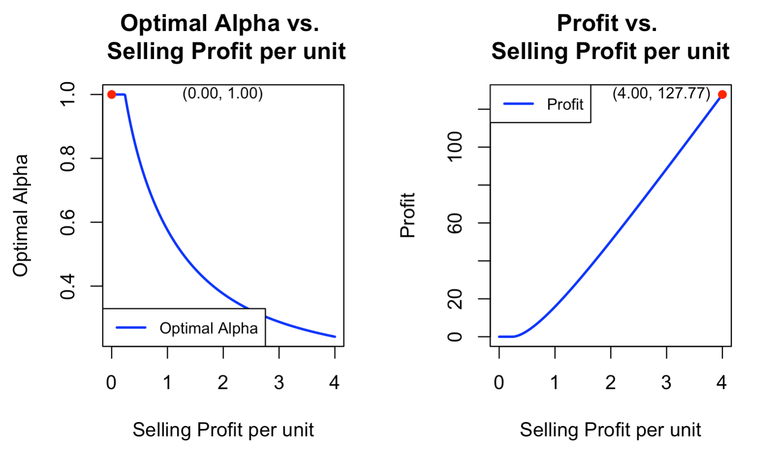
Figure 1: Optimal Level of Alpha and Profit Graph w.r.t. $p-c$

Effect of Increasing Carbon Prices ($B$) on Optimal Alpha (Figure 2)

As shown in Figure 2, when the carbon pricing variable $B$ increases, it raises operational costs for the firm due to higher carbon taxes. In response, the optimal investment ratio $\alpha$ also increases, as shown in the left plot. This adjustment indicates a strategic move by the firm to allocate more resources towards low-carbon transition initiatives, which enhances production efficiency and reduces carbon emissions, thereby helping to offset the financial burden imposed by the carbon tax.

However, the right plot shows that despite these adjustments, a higher carbon tax still leads to a reduction in overall profit. Even with an optimal increase in the low-carbon investment ratio $\alpha$, the profit trend declines as $B$ increases. This underscores the financial impact of rising carbon costs on the firm. Nonetheless, by investing strategically in low-carbon transition, the firm can mitigate the extent of this profit decrease, cushioning some of the adverse effects of carbon pricing. In essence, while higher carbon taxes inevitably compress profits, allocating resources towards reducing the carbon footprint can help alleviate the downward pressure on profitability, offering a partial buffer against the increasing tax burden.

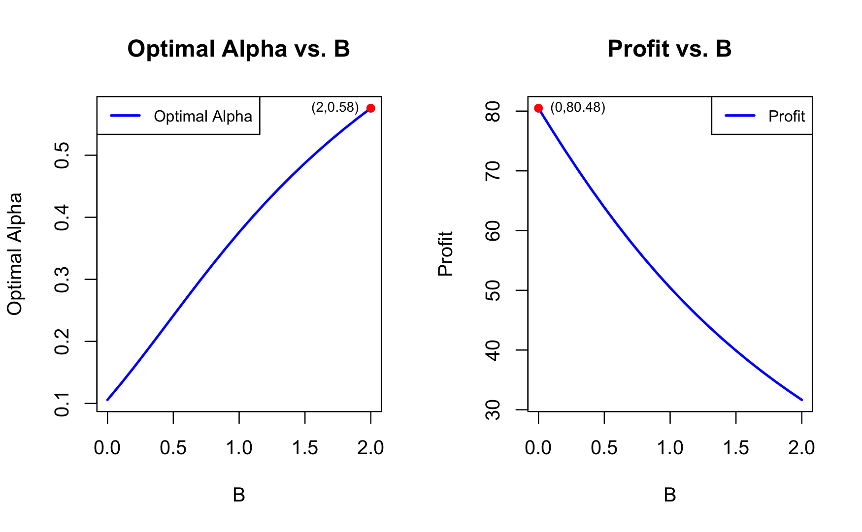
Figure 2: Optimal Level of Alpha and Profit Graph w.r.t. $B$

Impact of Efficiency Parameter ($k$) on Optimal Alpha and Profit (Figure 3)

Combining insights from both plots in Figure 3, we can observe that as the efficiency parameter $k$ increases, profit consistently rises, while the optimal investment ratio $\alpha$ peaks around $k\approx 3.1$ and then gradually declines. This suggests that although higher $k$ values are beneficial for the company’s profitability, it does not require continuously increasing the investment ratio in low-carbon initiatives. Initially, when $k$ is low, the marginal benefit from efficiency gains is high, encouraging a higher allocation to low-carbon investments. However, as $k$ grows, the marginal efficiency gains diminish, making it less necessary to maintain a high $\alpha$. At higher $k$ values, profits continue to increase due to the enhanced production efficiency achieved by prior investments, allowing the company to reduce the investment ratio $\alpha$ while still benefiting from increased profits.

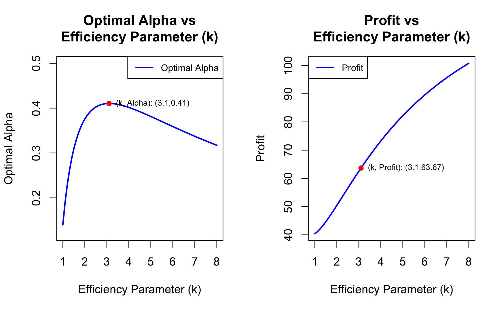
Figure 3: Optimal Level of Alpha and Profit Graph w.r.t. $k$

Influence of Original Productivity Coefficient ($\beta$) on Optimal Alpha and Profit (Figure 4)

The plots in Figure 4 demonstrate that as the Original Productivity Coefficient ($\beta$) increases, profit grows exponentially while the optimal transition investment ratio ($\alpha$) declines. A higher $\beta$ indicates strong baseline productivity, reducing the need for extensive low-carbon investments since the firm’s production efficiency is already high. This makes the additional benefits from low-carbon investments less significant, allowing the firm to allocate fewer resources to $\alpha$. The exponential growth in profit with rising $\beta$ highlights the significant impact of inherent productivity on profitability, as firms with high baseline efficiency can achieve substantial profits without heavy investment in low-carbon initiatives. The decrease in optimal $\alpha$ reflects diminishing marginal returns on low-carbon investments for high-$\beta$ firms, where the benefits of further investment in $\alpha$ are minimal.

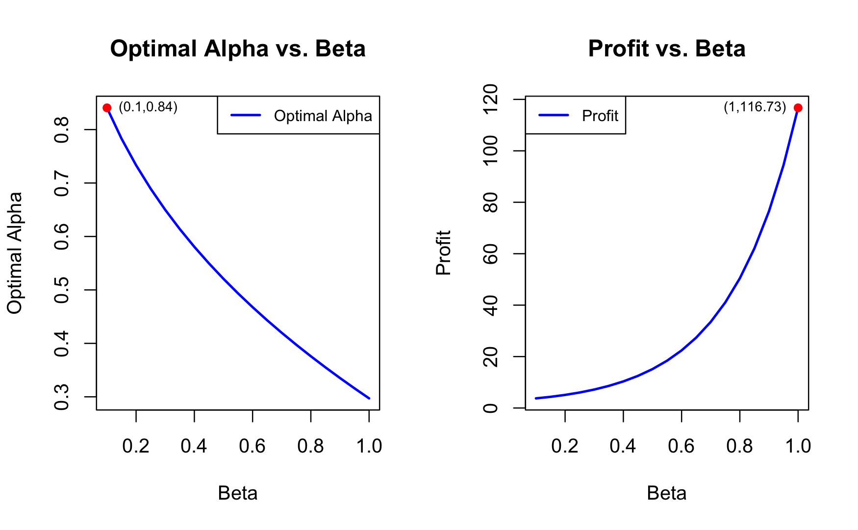
Figure 4: Optimal Level of Alpha and Profit Graph w.r.t. $\beta$

2.3.3 Sensitivity Analysis

The sensitivity analysis was conducted to evaluate the impact of variations in critical parameters on the optimal alpha, maximum objective value, and profit change rate. The parameters scrutinized include the enterprise low-carbon production efficiency coefficient ($k$), production cost per unit ($c$), original productivity coefficient ($\beta$), and carbon price per unit ($B$). Adjustments for each parameter were performed at ±10% and ±50% based on the baseline values in Table 2, except for $\beta$, where the upper limit was constrained to 1.00 due to inherent limitations. The results are concluded in the Table 3 and the analysis of each parameter is presented below.

$k$ (Enterprise Low-carbon Production Efficiency Coefficient)
Parameter Value	1.0	1.8	2.0	2.2	3.0
Optimal Alpha	0.1399250	0.3560002	0.3758660	0.3896782	0.4102122
Max Objective Value	40.38998	48.03570	50.43508	52.88084	62.52014
Alpha Change Rate (%)	-62.77263	-5.285352	0.000000	3.674763	9.137887
Profit Change Rate (%)	-19.916887	-4.757367	0.000000	4.849314	23.961613
$c$ (Production Cost Per Unit)
Parameter Value	0.80	1.44	1.60	1.76	2.40
Optimal Alpha	0.3011413	0.3571930	0.3758660	0.3970913	0.5191683
Max Objective Value	80.82201	56.40787	50.43508	44.53826	22.16245
Alpha Change Rate (%)	-19.880685	-4.967987	0.000000	5.647027	38.125899
Profit Change Rate (%)	60.249582	11.842530	0.000000	-11.69191	-56.05747
$\beta$ (Original Productivity Coefficient)
Parameter Value	0.40	0.72	0.80	0.88	1.00
Optimal Alpha	0.5806144	0.4107206	0.3758660	0.3430713	0.2971025
Max Objective Value	10.33973	36.31521	50.43508	70.34946	116.72607
Alpha Change Rate (%)	54.473780	9.273146	0.000000	-8.725114	-20.955217
Profit Change Rate (%)	-79.49894	-27.99613	0.000000	39.48516	131.43825
$B$ (Carbon Price Per Unit)
Parameter Value	0.5	0.9	1.0	1.1	1.5
Optimal Alpha	0.2414888	0.3505336	0.3758660	0.4002088	0.4874011
Max Objective Value	63.88578	52.87325	50.43508	48.11505	39.90827
Alpha Change Rate (%)	-35.751365	-6.739751	0.000000	6.476445	29.674174
Profit Change Rate (%)	26.669326	4.834262	0.000000	-4.600030	-20.871997

Table 3: Sensitivity Analysis Results

Enterprise Low-Carbon Production Efficiency Coefficient $(k)$ :

The sensitivity analysis for $k$ reveals that as $k$ increases from 1.0 to 3.0, the optimal alpha rises from 0.14 to 0.41, which indicates that improving a firm’s low-carbon production efficiency encourages a larger investment by the firm in low-carbon technologies. This trend is further reflected in the maximum objective value, which grows from 40.39 to 62.52, showing that better firm’s efficiency leads to higher profitability for the firm. These results highlight a strong connection between firm’s low-carbon production efficiency and its profitability.

Moreover, the alpha change rate starts with a large negative value (-62.77%) when $k=1.0$ and makes a transition to a moderately positive change of $9.14\%$ by $k=3.0$. Similarly, the firm’s profit change rate shifts from a notable loss ($-19.92\%$) at $k=1.0$ to a relatively large gain $(23.96\%$) at $k=3.0$. This indicates that as efficiency improves, firms not only increase their levels of investment in cleaner technologies but also experience greater profitability. These results underline the importance of improving low-carbon production efficiency, as it can serve as a key driver for both firm’s optimal investment and its profit maximization.

Production Cost Per Unit (c):

As $c$ increases from 0.80 to 2.40, the optimal alpha rises from 0.30 to 0.52, suggesting that firms must invest more to counterbalance higher production costs. However, this comes at the cost of its profitability, as the maximum objective value drops sharply from 80.82 to 22.16, showing that rising production costs significantly undermine a company’s profitability potential.

The alpha change rate starts at $-19.88\%$ for $c=0.80$, meaning that lower production costs lead to less investment in low-carbon technology. As $c$ rises, the alpha change rate becomes positive (38.13%), showing that companies need to increase their investments to cope with higher costs. Profit change rates, meanwhile, vary drastically, reaching a peak at $60.25\%$ for $c=0.80$, followed by a steep decline to $-56.06\%$ at $c=2.40$. This result illustrates the sensitivity of firm’s profitability to changes in its production costs and highlights that controlling production costs is crucial for firms whose goal is to sustain profits while investing in low-carbon solutions. If its production costs rise unchecked, the firm may struggle to maintain its profitability, even with optimal investments.

Original Productivity Coefficient $(\beta)$ :

When it comes to the value of $\beta$, the sensitivity analysis overall shows a unique pattern: as $\beta$ increases from 0.40 to 1.00, the optimal alpha decreases from 0.58 to 0.30. This indicates that as its productivity improves, the firm requires less investment in low-carbon technologies to maintain profitability. Simultaneously, the maximum objective value surges from 10.34 to 116.73, highlighting the substantial impact of productivity on overall profitability of the firm. This result emphasizes that improving productivity not only reduces the required investment by the firm but also dramatically boosts the firm’s profit potential.

The change rate of alpha starts at a high level (54.47%) when $\beta=0.40$ and drops to $-20.96\%$ at $\beta=1.00$, showing that better productivity substantially reduces the need for the firm to increase the level of investment. In terms of profitability, the profit change rate for the firm ranges widely, from $-79.50\%$ to a remarkable $131.44\%$. This further illustrates how vital firm’s productivity improvements are for enhancing its profitability. Essentially, better productivity allows firms to generate substantially higher profits with a reduced level of investment, making this an essential factor in optimizing their financial strategies of the firm.

Carbon Price Per Unit $(B)$ :

Finally, the analysis of $B$ shows that as carbon prices increase from 0.50 to 1.50, the optimal alpha rises from 0.24 to 0.49, suggesting that the firm needs to allocate more resources to low-carbon production as carbon prices rise. However, this comes at a cost, as the maximum objective value declines from 63.89 to 39.91, showing that higher carbon prices can lead to a reduced level of profitability.

The change rate of alpha is consistently negative, starting at $-35.75\%$ for $B=0.50$ and improving slightly to $-6.74\%$ at $B=1.10$, indicating that while increased carbon pricing necessitates the firm to invest more, its negative impact on profitability is relatively moderate. The change rate of the profit peaks at $26.67\%$ for $B=0.50$ and drops to $-20.87\%$ at $B=1.50$. This suggests that while carbon pricing does affect firm’s profitability, the sensitivity is not as severe for the firm compared to other variables. Companies can mitigate the impact of higher carbon prices through improved efficiency and strategic investments in cleaner technologies, ensuring that their profitability does not drastically diminish as carbon prices rise.

In comparing the variables in the framework, it is clear that the original productivity coefficient $(\beta)$ is by far the most sensitive. Changes in the value of $\beta$ lead to substantial shifts in the optimal value of alpha, maximum objective value, and the change rate of the profit. The strong relationship between productivity and profitability suggests that firms should prioritize improving productivity to maximize financial outcomes.

Conversely, the carbon price per unit $(B)$ is the least sensitive variable in the framework. While changes in $B$ do affect both the optimal alpha and the profitability, the overall impact for the firm is moderate compared to the other factors. Firms can manage the effects of carbon pricing through strategic investments in cleaner technologies, making it a more controllable factor in its financial performance.

In conclusion, firms should focus heavily on productivity improvements $(\beta)$ to maximize their profitability while carefully managing their production costs $(c)$ and their low-carbon production efficiency ($k$) to optimize investments. Carbon pricing $(B)$, while important, presents a more manageable challenge to firms relative to the other factors.

2.3.4 Expanding the One-Period Model to a Multi-Period Model

In our initial analysis, we have focused on a static one-period model to evaluate the impact of transition investment on enterprise profitability. This framework provided basic but useful insights into the immediate effects of various variables on a company’s profit. However, real-world scenarios are dynamic in nature and involve changes over multiple periods. Therefore, as a next logical step, we are expanding our previous static framework to a multi-period setting to capture the evolving nature of the variables in the framework and their long-term impacts.

To achieve this, we revise the profit function to account for time dependency, reflecting the changes in key variables in the framework over multiple different periods. The time-dependent profit function is defined as follows:

$$\pi_{t}=\left[p-c_{t}-\left(\frac{2e^{-\alpha k_{t}}}{1+e^{-\alpha k_{t}}}\right)\times B_{t}\right]\times\left[\frac{2}{1+e^{-\alpha k_{t}}}\times\left[(1-\alpha)\cdot A_{t}\right]^{\beta_{t}}\right]$$ (2.6)

This formulation captures the dynamic nature of transition investments, where $p$ is the selling price per unit (assume $p$ is a constant), $c_{t}$ is the production cost per unit at time $t,\alpha$ is the transition investment ratio, $k_{t}$ is the enterprise low-carbon production efficiency coefficient at time $t,B_{t}$ is the carbon price at time $t$, and $\beta_{t}$ is the original productivity coefficient at time $t$. By incorporating these time-dependent variables, we can more accurately model the impact of transition investments over multiple periods.

The resulting multi-period objective function can then be expressed as follows:

$$\max\left[\pi_{t}+g\pi_{t+1}+g^{2}\pi_{t+2}+\ldots+g^{n-1}\pi_{t+n}\right]$$ (2.7)

where $g$ is the discount factor. This objective function accounts for firm’s profits in the current period $\left(\pi_{t}\right)$ and its discounted future profits ($\pi_{t+1},\pi_{t+2}$, and so on), providing a more complete view of the impact of transition investments for the firm. The inclusion of future profits, discounted to the present time by the factor $g$, acknowledges the time value of money, opportunity costs, and inherent risks faced by the company. The discounting factor also acknowledges the uncertainties associated with long-term projections, ensuring a realistic assessment of the enterprise’s financial trajectory.

By using this multi-period framework, we aim at finding the optimal value of $\alpha$ that maximizes the overall profit of the firm across multiple periods. The multi-period model is particularly useful for understanding the long-term implications of transition investments for the firm. Transitional investments typically incur immediate costs but generate substantial future benefits for the firm. For example, investments in low-carbon technologies might initially increase production costs for the firm due to the capital expenditure required for new equipment or processes. However, over time, these investments can lead to substantial efficiency gains, cost reductions, and improved regulatory compliance, which enhance future profits of the company.

Short-Term vs. Long-Term Observation:

Our goal is to find the optimal value of $\alpha$ to achieve the maximum objective function value for the firm over different observation periods. For simplicity, we will compare a shorter-term observation (of 3 years) with a longer-term observation (of 6 years).

• Short-Term Observation (3 years): This period allows us to understand the immediate and near-future impacts of transition investments for the firm. It is suitable for enterprises looking for quick wins and immediate adjustments in their strategies.

• Long-Term Observation (6 years): This extended period captures the long-term benefits and potential drawbacks of transition investments faced by the company. It helps the enterprises’ plan strategically for sustained growth and ensures compliance with evolving regulations and market conditions.

By comparing these two observation periods, we can evaluate how the optimal value of $\alpha$ varies based on the length of the planning horizon for the company. This comparison will provide important insights into the trade-offs between short-term gains and long-term sustainability, guiding enterprises in making informed decisions about their transitional investments. The numerical exercise will be presented in the next subsection to illustrate these findings.

2.4 Decarbonization Scenario Analysis

2.4.1 Introduction to Decarbonization Scenarios

To illustrate the practical application of our multi-period framework, we examine four decarbonization scenarios by means of a numerical method: Immediate, Quick, Slow, and No Decarbonization. Decarbonization scenarios are strategic frameworks used to explore and analyze the pathways by which industries, economies, and societies can make a transition from high-carbon to low-carbon or carbon-neutral operations. These scenarios are designed to address the urgent need to mitigate climate change by reducing GHG emissions, particularly carbon dioxide (CO2), which is viewed as a major contributor to human-induced global warming. Each decarbonization scenario represents a different approach, pace, and scale of implementing low-carbon technologies, policies, and practices.

These scenarios draw inspiration from the pathways outlined in IPCC’s Representative Concentration Pathways (RCPs) and Shared Socioeconomic Pathways (SSPs) (IPCC (2018, 2022)), which provide a framework for modeling emissions trajectories under varying socio-economic, policy, and technological conditions. For example, the Immediate Decarbonization scenario aligns with the stringent measures seen in RCP1.9/SSP1-1.9, where immediate, large-scale investments aim to limit global temperature rise to 1.5°C (IPCC (2018)). Conversely, the No Decarbonization scenario parallels RCP8.5/SSP5-8.5, representing a ”business-as-usual” trajectory with minimal climate action and escalating carbon emissions (IPCC (2023)).

By analyzing these different scenarios, we can better understand how decarbonization strategies impact enterprise profitability over multiple periods and identify the optimal transition investment ratio ($\alpha$) for each strategy.

Immediate Decarbonization:

In this scenario, significant and immediate investments are made in low-carbon technologies and practices. The goal is to achieve rapid reductions in carbon emissions as quickly as possible. This approach mirrors the aggressive pathways described in RCP1.9/SSP1-1.9, where rapid decarbonization is pursued through stringent regulatory measures, substantial financial incentives, and rapid deployment of renewable energy and energy efficiency technologies (IPCC (2018)). Immediate decarbonization is typically driven by strong political will and societal urgency to address climate change impacts swiftly. While effective in achieving fast emissions reductions, it may entail higher short-term costs and risks of over-investment.

Quick Decarbonization:

Quick Decarbonization involves a fast-paced yet balanced transition. Investments in low-carbon technologies are substantial but spread out over a few years rather than all at once. This scenario resembles the pathways described in RCP2.6/SSP1-2.6, where emissions reductions are significant but distributed over time to balance economic feasibility and technical constraints (IPCC (2022); Agency (2022)). Quick decarbonization includes strategies such as accelerated deployment of renewable energy, electrification of transportation, and enhanced energy efficiency measures. It offers a cost-effective and pragmatic approach to achieving climate goals while reducing the economic and logistical burden of an immediate overhaul.

Slow Decarbonization:

The Slow Decarbonization scenario adopts a more gradual approach to transitioning to a low-carbon economy. Investments and regulatory changes are implemented over a longer period of time, allowing for a smoother transition with less immediate economic disruption. This approach corresponds to RCP4.5/SSP2-4.5, a “middle-of-the-road” pathway where moderate policies and socio-economic factors lead to incremental emissions reductions over time (IPCC (2023)). While less disruptive, this scenario risks delaying critical action, potentially increasing long-term mitigation costs and reliance on future technological breakthroughs.

No Decarbonization:

In the No Decarbonization scenario, no substantial efforts are made to reduce carbon emissions. This approach parallels the ”business-as-usual” trajectory represented by RCP8.5/SSP5-8.5, where industries and societies continue with their current high-carbon practices (IPCC (2018)). Continued reliance on fossil fuels results in escalating carbon emissions, environmental degradation, and increased climate risks (Agency (2022); IPCC (2023)). This scenario is widely regarded as unsustainable, as it amplifies the adverse economic, environmental, and social impacts of climate change over time.

2.4.2 Variable Changes and Rationale for Each Decarbonization Scenario

To effectively analyze the aforementioned impacts of different decarbonization strategies, it is essential to understand how key variables in the framework evolve under each scenario and the rationale behind these changes. This part delves into the specific modifications of variables such as the enterprise low-carbon production efficiency coefficient $\left(k_{t}\right)$, production cost per unit ($c_{t}$), original productivity coefficient ($\left.\beta_{t}\right)$, and carbon price $\left(B_{t}\right)$ for each of the decarbonization scenarios: Immediate, Quick, Slow, and No Decarbonization. By doing so, we can better comprehend the short-term and long-term effects of the transition on firm’s profitability and identify the optimal transition investment ratio $(\alpha)$ for the firm in each case.

Immediate Decarbonization:

In the Immediate Decarbonization scenario, enterprises make substantial investments in low-carbon technologies immediately. This aggressive approach aims at achieving rapid decarbonization and substantial reductions in carbon emissions in the shortest possible time. As a result, the enterprise’s low-carbon production efficiency coefficient $\left(k_{t}\right)$ starts at a very high level due to a substantial initial level of investment, reflecting major improvements in production efficiency of the firm. Over time, as the immediate benefits are realized, $k_{t}$ decreases gradually. The production cost per unit $\left(c_{t}\right)$ of the firm decreases quickly as economies of scale and technological efficiencies are realized from the new low-carbon technologies. The original productivity coefficient $\left(\beta_{t}\right)$ increases initially due to enhanced production capabilities of the firm but stabilizes over time as the effects of initial investments are more fully integrated. The carbon price ($B_{t}$) remains at a very high level due to stricter regulations and market adjustments that favor low-carbon outputs.

Quick Decarbonization:

The Quick Decarbonization scenario involves rapid but slightly less aggressive investments compared to the Immediate scenario. Enterprises aim at achieving substantial decarbonization within a relatively short time frame but spread their investments over a few periods of time to balance costs and benefits. Consequently, the enterprise’s low-carbon production efficiency coefficient $\left(k_{t}\right)$ increases quickly but not as sharply as in the case of the Immediate scenario. The efficiency gains are substantial for the firm but spread over a slightly longer period of time. The production cost per unit $\left(c_{t}\right)$ decreases rapidly but not as dramatically, reflecting more moderate cost reductions. The original productivity coefficient $\left(\beta_{t}\right)$ shows a steady increase due to technological improvements and better resource allocation by the firm. The carbon price $\left(B_{t}\right)$ keeps at a relatively high level, driven by increasing regulatory pressures and market responses.

Slow Decarbonization:

In the Slow Decarbonization scenario, enterprises adopt a gradual approach to transitioning to low-carbon technologies. This approach spreads investments over a longer period of time, allowing enterprises to manage costs and mitigate risks while steadily reducing carbon emissions. As such, the enterprise’s low-carbon production efficiency coefficient $\left(k_{t}\right)$ increases slowly, reflecting incremental improvements in production efficiency for the firm as investments are made gradually. The production cost per unit $\left(c_{t}\right)$ decreases steadily but slowly, indicating progressive cost reductions over time. The original productivity coefficient $\left(\beta_{t}\right)$ shows a gradual increase, correlating with incremental enhancements in productivity as new technologies are adopted by the firm over time. The carbon price $\left(B_{t}\right)$ is set as a relatively low level, aligning with gradual regulatory changes and market adjustments.

No Decarbonization:

The No Decarbonization scenario assumes that enterprises do not make any major investments in low-carbon technologies. Instead, they continue with their current practices, resulting in minimal changes to carbon emissions and production efficiency. Consequently, there is no need to find the optimal transitional investment ratio under this scenario, as the transitional investment ratio, $\alpha$, should always be zero.

2.4.3 Numerical Study

By analyzing these different scenarios, we can observe how different levels of investment and urgency in transitioning to low-carbon technologies affect key variables of the framework over time. This analysis helps us understand the trade-offs between immediate costs and long-term benefits, guiding enterprises in making informed decisions about their decarbonization strategies. The goal is to determine the optimal value of $\alpha$ that maximizes the overall profit across multiple periods, ensuring both short-term (3-year observation period) profitability and long-term (6-year observation period) sustainability. We will not consider the scenario of ‘No Decarbonization’ in this part, as there is no need to determine the optimal transitional investment ratio $\alpha$ under this scenario.

Year	1	2	3	4	5	6
$k$ (Enterprise Low-carbon Production Efficiency Coefficient)
Immediate	5	4.5	4	3.5	3	2.5
Quick	1.5	5	4.5	4	3.5	3
Slow	2	3	4	5	4.5	4
$c$ (Production Cost Per Unit)
Immediate	1.6	1.7	1.8	2	2.2	2.4
Quick	2.4	1.6	1.7	1.8	2	2.2
Slow	2.2	1.9	1.6	1.7	1.8	2
$\beta$ (Original Productivity Coefficient)
Immediate	0.9	0.85	0.8	0.75	0.72	0.7
Quick	0.6	0.9	0.85	0.8	0.75	0.72
Slow	0.7	0.8	0.9	0.85	0.8	0.75
$B$ (Carbon Price Per Unit)
Immediate	4	4	4	4	4	4
Quick	3	3	3	3	3	3
Slow	2	2	2	2	2	2

Table 4: Results for Scenario Analysis

Table 4 presents various variables under different scenarios of low-carbon transition for enterprises, focusing on production efficiency, costs, productivity, and carbon pricing.

In the Immediate Transition scenario, enterprises rapidly adopt low-carbon technologies, leading to a substantial increase in firm’s production efficiency initially. This efficiency gain diminishes over time due to the fast adaptation rate and potential initial over-investment by the firm, as reflected in the decreasing values of the enterprise’s low-carbon production efficiency coefficient $k$. Production costs per unit rise initially due to high investments in new technologies, reaching their peak in later years as the benefits of the new technologies become more apparent and grounded. The original productivity coefficient $\beta$ sees a rapid decrease due to the initial disruption and learning curve of the firm associated with adopting new technologies, eventually stabilizing at a lower level over time. High carbon pricing ($B$) is a crucial factor in this scenario, as it works to incentivize the rapid adoption of low-carbon technologies to mitigate the associated costs.

In the Quick Transition scenario, enterprises adopt low-carbon technologies at a moderately fast pace. This approach aims at achieving a rapid improvement in production efficiency, though at a slightly slower rate than in the Immediate scenario. As a result, the initial efficiency gains are significant but not as drastic, allowing the enterprise to avoid potential issues related to over-investment. Given the initially low value of $k$ (starting at 1.5), there is an urgent need to enhance production efficiency quickly. To address this, the enterprise makes a transition investment before the second year, resulting in a sharp increase in $k$ to 5 by the second year. This value then gradually declines each subsequent year, reflecting the natural efficiency losses due to wear and tear. Production costs per unit begin at a relatively high level (2.4), creating a strong need for transition investment to reduce costs. With the Quick Decarbonization approach, $c$ drops significantly to 1.6 in the second year. However, it then rises slightly in the following years, likely due to normal depreciation and the ongoing costs associated with maintaining the new technology. Similarly, the original productivity coefficient $\beta$ starts at a lower level (0.6), emphasizing the necessity for improvement. Due to the transition investment, $\beta$ reaches a peak of 0.9 in the second year, reflecting increased productivity. Over time, it gradually decreases, aligning with the adaptation phase and the natural reduction in productivity gains. Carbon pricing $B$ is maintained at a high but stable level (3) in the Quick Decarbonization scenario. This provides a continuous incentive for adopting low-carbon technologies, without imposing excessive financial burdens on the firm.

In the Slow Transition scenario, enterprises adopt low-carbon technologies at a gradual pace, resulting in a steady increase in production efficiency without abrupt changes. The Enterprise Low-carbon Production Efficiency Coefficient ($k$) begins at a modest value of 2 and gradually rises to 5 by the fourth year before leveling off slightly, indicating a more controlled and gradual improvement. This slower adoption rate minimizes the impact of efficiency losses due to wear and tear over time. The Production Cost Per Unit ($c$) starts relatively high at 2.2 but decreases progressively as the benefits of low-carbon technology adoption become more apparent, reaching a stable level at 1.8 by the final year. Such a pattern reflects slower capital outlays and reduced urgency in operational adjustments, leading to consistent long-term savings. The Original Productivity Coefficient ($\beta$) also starts at a low value of 0.7 and improves steadily to a peak of 0.9 in the third year, maintaining stability thereafter. This steady incline suggests a smoother, less disruptive learning curve associated with gradual integration of new technologies. Finally, the Carbon Price Per Unit ($B$) remains low at 2 throughout the period, applying gentle pressure on firms to adopt low-carbon technologies while allowing them to adjust at a manageable pace, balancing the transition costs with sustained incentives.

The simulation results in Table 5 reveal an intriguing insight into the relationship between decarbonization strategies and firm profitability over different time horizons. In the short term, the Immediate decarbonization scenario yields the highest profits for the firm, while in the long term, profits are maximized under the Slow decarbonization strategy. The economic intuition behind this pattern lies in the interplay between the upfront investment requirements, efficiency gains, and financial planning associated under the different decarbonization strategies.

	Short-Period		Long-Period
	Optimal $\alpha$	Max Profit	Optimal $\alpha$	Max Profit
Immediate	0.5692	173.0291	0.6216	212.0262
Quick	0.541	158.3299	0.5678	235.1407
Slow	0.4768	131.7251	0.4606	261.1729

Table 5: Optimal Investment Ratio and Max Profit for Short-Period and Long-Period Scenarios

In the short term, Immediate decarbonization leads to high profits because it allows the firm to achieve early efficiency gains and cost savings from the rapid adoption of low-carbon technologies. By quickly reducing energy and resource inefficiencies, the firm can capitalize on immediate cost reductions, enhanced operational performance, and potentially favorable regulatory incentives for early movers in decarbonization. These benefits outweigh the initial financial burden of the transition, resulting in the highest short-term profitability.

However, in the long term, the economic dynamics inevitably shift. The substantial upfront costs associated with Immediate decarbonization, including significant investments in low-carbon technologies and potential disruptions to existing operations, begin to erode long-term profitability. These high initial costs reduce the firm’s capacity to sustain investments and adapt to evolving market and regulatory conditions over time. In contrast, the Slow decarbonization scenario allows the firm to distribute its transition costs more evenly over a longer period. This gradual approach minimizes financial strain, enhances the firm’s ability to adapt incrementally, and provides a greater degree of flexibility to optimize investments as low-carbon technologies become matured and more cost-effective. As a result, the Slow strategy enables the firm to achieve a higher long-term profitability. The Quick scenario represents a middle ground between Immediate and Slow strategies. In the short term, its profitability is lower than Immediate decarbonization due to moderate initial costs and slower realization of efficiency gains. However, in the long term, Quick decarbonization surpasses the Immediate scenario in profitability, as it balances higher levels of initial investments with a sufficient degree of flexibility to adapt and sustain low-carbon operations.

Overall, the results highlight the importance of strategic planning in decarbonization efforts. Firms must weigh the trade-offs between short-term efficiency gains and long-term financial stability when determining their optimal transitional investment ratios. While Immediate decarbonization may deliver immediate benefits, a gradual approach such as the Slow strategy offers a more sustainable path to maximizing long-term profits and resilience. This underscores a critical role of proactive, well-paced investment planning in achieving both financial and sustainability goals.

2.5 Optimal Transition Investment Ratio with Government Intervention

Based on the conclusions drawn from the previous subsections, it is evident that companies may exhibit a deficiency in transformational investments in certain scenarios. In such instances, it becomes especially relevant for the government to undertake steps of market adjustments at both macro and micro levels, employing tools such as subsidies or tax penalties.

Subsidies can serve as a powerful incentive for companies by lowering the financial burden associated with making a transition to low-carbon technologies. These subsidies can take various forms, such as direct financial assistance, tax credits, or grants for research and development in green technologies. By reducing the initial costs, subsidies make low-carbon investments more attractive to companies, thereby accelerating the adoption of sustainable practices. For example, a company might receive a tax credit for every unit of renewable energy produced, which would directly offset its production costs and enhance profitability.

On the other hand, tax penalties act as a deterrent against environmentally harmful practices. By imposing higher taxes on carbon emissions or non-compliant activities, governments can create the risk of a financial disincentive for companies to continue with high-carbon operations. This approach compels businesses to internalize the environmental costs of their actions, thereby encouraging them to seek out more sustainable alternatives. For instance, a carbon tax that increases with the level of emissions will drive companies to innovate and invest in cleaner technologies to minimize their tax liabilities.

Governments have a vested interest in incentivizing companies to undertake low-carbon transitions for several important reasons. Firstly, fostering a transition to low-carbon practices aligns with broader environmental and climate goals, mitigating the adverse effects of climate change and reducing overall carbon emissions in the country. Secondly, by encouraging businesses to adopt sustainable practices, governments contribute to the development of a more resilient and environmentally conscious economy. Additionally, promoting low-carbon transitions enhances a country’s global competitiveness by positioning it as a leader in clean and sustainable technologies. This, in turn, attracts environmentally conscious investments, boosts innovation, and creates green jobs, fostering economic growth. Furthermore, by mitigating environmental risks and promoting sustainability, governments aim at improving public health and reduce the strain on healthcare systems in the country. Incentivizing low-carbon transitions therefore reflects a strategic approach to building a more sustainable and prosperous future, where economic development is harmonized with environmental stewardship.

2.5.1 Model Building

In the extended framework below, we categorize government regulatory tools into two groups: one from a macro-economic perspective and the other from a micro-economic perspective. The government acts as an ‘invisible hand’. We assume that from a macro-economic perspective, the government subsidizes carbon prices that are too high in the market and taxes carbon prices that are too low in the market. On a micro-economic level, if a company surpasses a specified threshold for carbon emissions, the government levies taxes. Conversely, if a company’s total emissions fall below the threshold, the government offers rewards and subsidies to companies, fostering increased enthusiasm for low-carbon transformation initiatives. To introduce the extension model of the the previous framework, additional variables and parameters are introduced to be described in Table 6.

Notation	Description
$s_{1}$	Subsidy Rate for High Carbon Price
$s_{2}$	Subsidy Rate for Low Carbon Emission
$q_{1}$	Tax Rate for Low Carbon Price
$q_{2}$	Tax Rate for High Carbon Emission
$pr_{1}=Pr(\text{ Carbon Price}(B)\geqslant cp)$	Probability of Subsidy for High Carbon Price
$pr_{2}=Pr(\text{ Carbon Emission}\leqslant ce)$	Probability of Subsidy for Low Carbon Emission

Table 6: Variable and Parameter Description for the Extended Framework

Based on these variables and parameters, the expected total profit of the company after government subsidy or tax can be expressed as:

$$\pi^{\prime}=\pi +s_{1}\cdot(\text{ Total Unit Amount })\cdot pr_{1}-q_{1}\cdot(\text{ Total Unit Amount })\cdot\left(1-pr_{1}\right)$$ (2.8)

$$+s_{2}\cdot(\text{ Carbon Emission })\cdot pr_{2}-q_{2}\cdot(\text{Carbon Emission })\cdot\left(1-pr_{2}\right)$$

$$=\pi +s_{1}\cdot\left\{\left(\frac{2}{1+e^{-\alpha k}}\right)\cdot[(1-\alpha)\cdot A]^{\beta}\right\}\cdot pr_{1}-q_{1}\cdot\left\{\left(\frac{2}{1+e^{-\alpha k}}\right)\cdot[(1-\alpha)\cdot A]^{\beta}\right\}\cdot\left(1-pr_{1}\right)$$

$$+s_{2}\cdot\left(2-\frac{2}{1+e^{-\alpha k}}\right)\cdot\left\{\left(\frac{2}{1+e^{-\alpha k}}\right)\cdot[(1-\alpha)\cdot A]^{\beta}\right\}\cdot pr_{2}$$

$$-q_{2}\cdot\left(2-\frac{2}{1+e^{-\alpha k}}\right)\cdot\left\{\left(\frac{2}{1+e^{-\alpha k}}\right)\cdot[(1-\alpha)\cdot A]^{\beta}\right\}\cdot\left(1-pr_{2}\right)$$

where, the total profit $\pi$, excluding government intervention, is calculated as previously shown in Equation (2.3).

2.5.2 Numerical Study

In this subsection, we expand our analysis to explore the impact of government intervention on the optimal transition investment ratio $(\alpha)$ and profitability of the firm, through a revised objective function that incorporates both subsidies and taxes linked to carbon pricing and emissions. The new objective function, $\pi^{\prime}$, integrates additional terms representing financial incentives and penalties for the firm based on carbon-related metrics.

Our revised framework considers the following variables and parameters: subsidy rates ( $s_{1}$ and $s_{2}$ ) for high carbon prices and low carbon emissions, respectively; tax rates ( $q_{1}$ and $q_{2}$ ) for low carbon prices and high carbon emissions, respectively; and the probabilities ( $pr_{1}$ and $pr_{2}$ ) of these rates being applied based on carbon price and emission thresholds. These factors are critical for determining the cost-benefit landscape of environmental compliance and sustainable investment, as they directly influence the incentives and penalties faced by firms.

The baseline variables from our previous studies are maintained in this study for consistency, but now we add more variables and parameters to the framework. The baseline values for these new variables are shown in Table 7. Then we systematically vary each of the new variables and parameters individually to observe their effects on the optimal value of $\alpha$ and overall profitability for the firm. Graphical representations will be used to illustrate the relationship between these variables and the resulting economic outcomes, providing clear insights into the dynamics at play for the firm under different policy scenarios.

Notation	Description	Baseline Value
$s_{1}$	Subsidy Rate for High Carbon Price	0.8
$s_{2}$	Subsidy Rate for Low Carbon Emission	0.8
$q_{1}$	Tax Rate for Low Carbon Price	0.6
$q_{2}$	Tax Rate for High Carbon Emission	0.6
$pr_{1}$	Probability of Subsidy for High Carbon Price	0.5
$pr_{2}$	Probability of Subsidy for Low Carbon Emission	0.5

Table 7: New Baseline Values for Analysis

From Figure 5 to Figure 10, the left plot illustrates how changes in the key variable affect the optimal transition investment ratio, aiming to maximize profit under each scenario. The right plot shows the corresponding maximum profit achieved under the optimal transition investment as the key variable changes. We will explain each figure in detail below.

Impact of Probability of High Carbon Price Subsidy ($pr_{1}$) on Optimal Alpha and Profit (Figure 5)

As the probability of receiving a subsidy at higher carbon prices ($pr_{1}$) increases, the optimal investment ratio ($\alpha$) for the firm decreases. This suggests that businesses, when expecting financial support through subsidies, feel less pressure to invest heavily in low-carbon technologies. The security provided by expected subsidies reduces the need for extensive investment by the firm in hedging against future regulatory changes or market conditions that favor lower emissions. This also highlights a strategic point for businesses: relying too heavily on subsidies might provide a short-term relief but could risk an insufficient preparation for a future with stricter environmental regulations.

Profit increases alongside higher subsidy probabilities, reinforcing the positive impact of government incentives on financial performance of the firm. For investors, this underscores the appeal of firms with strong expectations of a subsidy support, as subsidies directly enhance profitability of the firm. However, it’s essential to remain cautious—companies that over-rely on subsidies may be less motivated to invest in long-term carbon reduction strategies, posing potential risks to the firm as market dynamics or regulations shift.

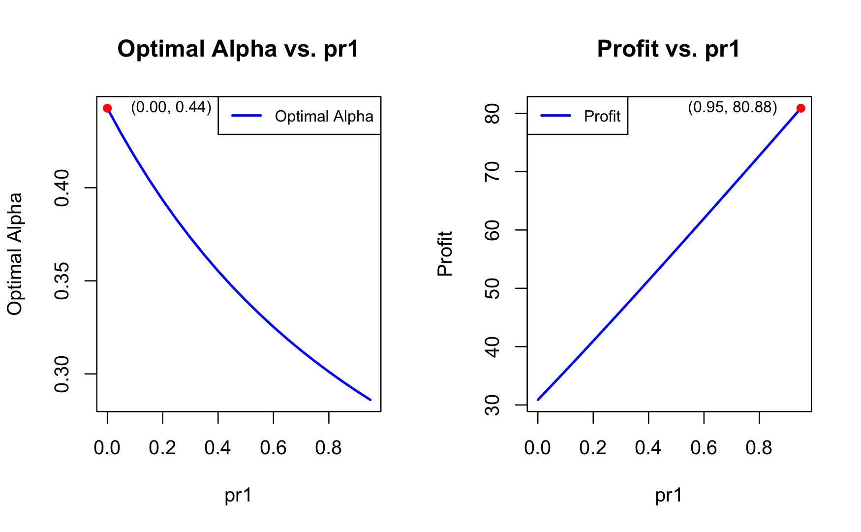
Figure 5: Optimal Level of Alpha and Profit Graph w.r.t. $pr_{1}$

Impact of Probability of Low Carbon Emission Subsidy ($pr_{2}$) on Optimal Alpha and Profit (Figure 6)

As $pr_{2}$ rises, it reflects a higher tolerance from the government for carbon emissions, effectively lowering the threshold required for firms to qualify for subsidies. This shift reduces the incentive for companies to invest in low-carbon transitions, as they can now receive financial support with less stringent emissions standards. Consequently, the optimal value of $\alpha$, which represents the proportion of resources allocated to low-carbon investments, declines. This trend shows that firms are less motivated to prioritize sustainable transitions when subsidies become more accessible without rigorous emission targets.

On the profitability side, a higher $pr_{2}$ initially appears to be advantageous. With reduced pressure to invest in transition efforts, firms can allocate fewer resources to low-carbon initiatives, which boosts short-term profits. However, this profit increase may be deceptive, as it comes at the expense of long-term resilience. Firms that minimize transition investments now could face significant financial risks if stricter carbon policies are introduced in the future. A sudden regulatory shift would leave them underprepared to adapt, potentially leading to substantial losses. This underscores the trade-off between short-term profit gains and the uncertain long-term stability that comes with underinvesting in sustainable practices.

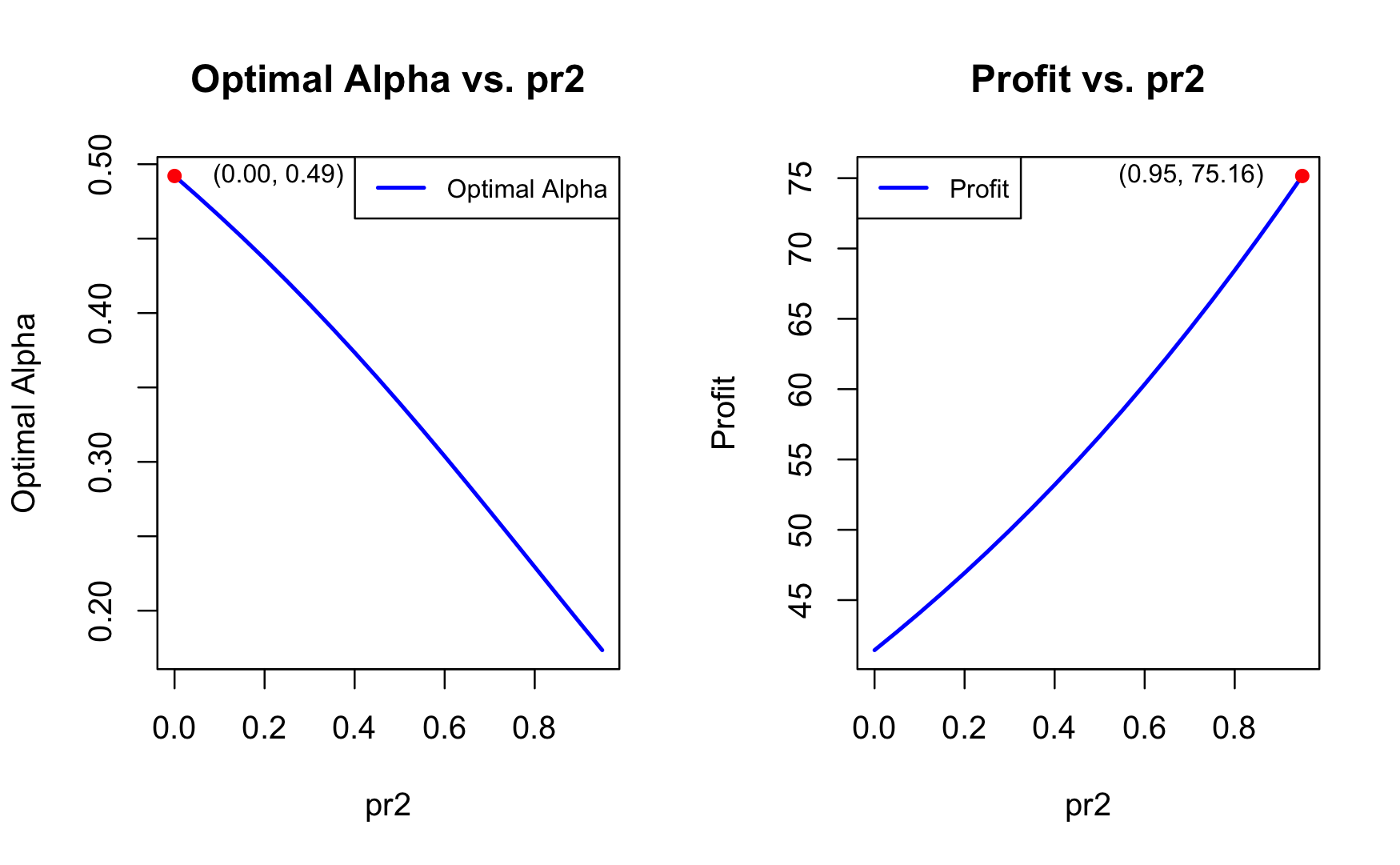
Figure 6: Optimal Level of Alpha and Profit Graph w.r.t. $pr_{2}$

Impact of Tax Rates for Low and High Carbon Emissions ($q_{1}$ and $q_{2}$) on Optimal Alpha and Profit (Figure 7 & Figure 8)

Higher tax rates on low carbon prices ($q_{1}$) or high carbon emissions ($q_{2}$) push the optimal value of $\alpha$ higher, indicating that businesses are incentivized to adopt cleaner technologies more aggressively when facing heavier tax burdens. This reflects the practical use of taxes as a tool for driving environmental sustainability—businesses react to them by increasing investments in green technologies to mitigate the financial impact of taxes. However, businesses must be strategic at the same time: while aggressive adoption of low-carbon technologies can reduce future tax liabilities for the firm, over-investing without aligning with long-term sustainability goals could lead to suboptimal resource allocation.

On the flip side, profits decrease as taxes rise, which makes high-emission activities less financially attractive for the firm. This highlights the financial risks for companies slow to adopt cleaner practices, reinforcing the need for a more proactive sustainability planning. Investors should be mindful of firms exposed to significant carbon taxes, as their profitability may suffer without adequate mitigation strategies.

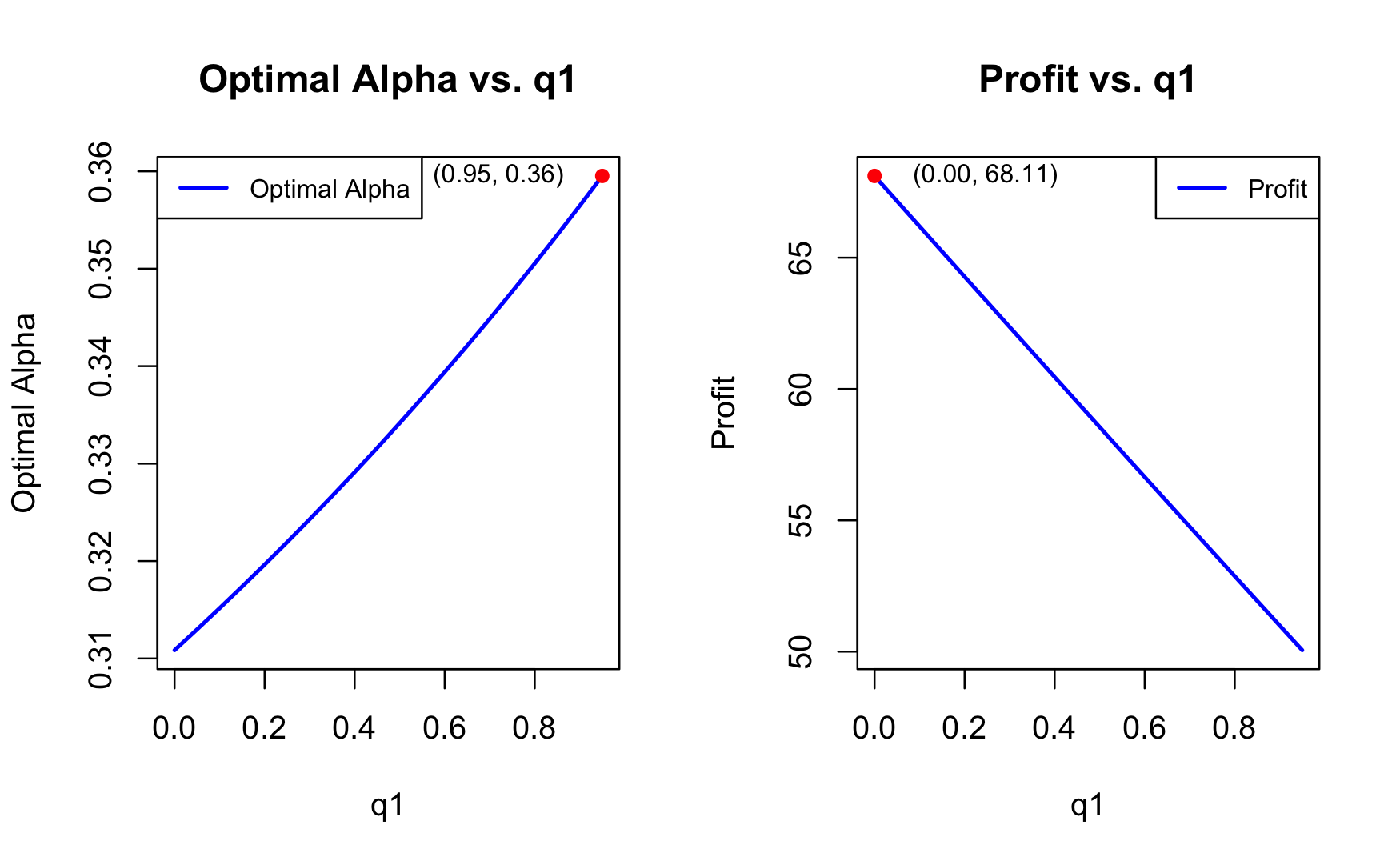
Figure 7: Optimal Level of Alpha and Profit Graph w.r.t. $q_{1}$

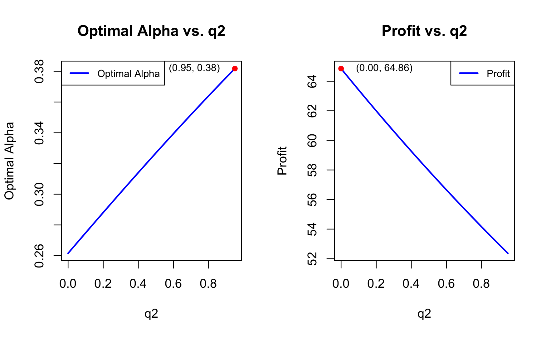
Figure 8: Optimal Level of Alpha and Profit Graph w.r.t. $q_{2}$

Impact of Subsidy Rates for High and Low Carbon Scenarios ($s_{1}$ and $s_{2}$) on Optimal Alpha and Profit (Figure 9 & Figure 10)

An increase in subsidy rates for high carbon price ($s_{1}$) or low carbon emission ($s_{2}$) scenarios results in a lower optimal value of $\alpha$, showing that businesses feel less urgency to invest heavily in green technologies when financial incentives make it easier to comply with emission standards. While this may seem beneficial for companies in the short term, there is a risk that such subsidies could slow down the transition to greener technologies if businesses rely too heavily on them without making the necessary levels of investment in long-term sustainability.

Profit increases with higher subsidies, emphasizing the role of financial support in boosting corporate earnings. From an investment perspective, firms with access to a substantial amount of subsidies for meeting environmental standards are likely to be more profitable in the short term, making them more appealing to investors. However, investors should also assess whether these companies are using the subsidy windfall to fund long-term sustainable transformations, as over-reliance on temporary fiscal incentives could pose challenges for the firm in the face of evolving market or regulatory conditions.

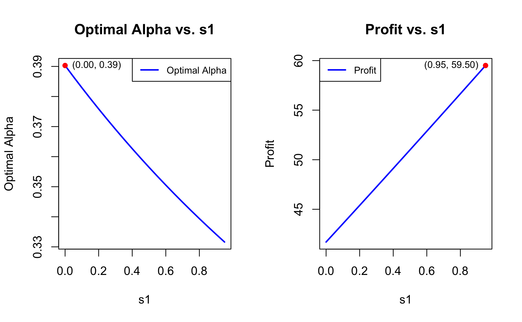
Figure 9: Optimal Level of Alpha and Profit Graph w.r.t. $s_{1}$

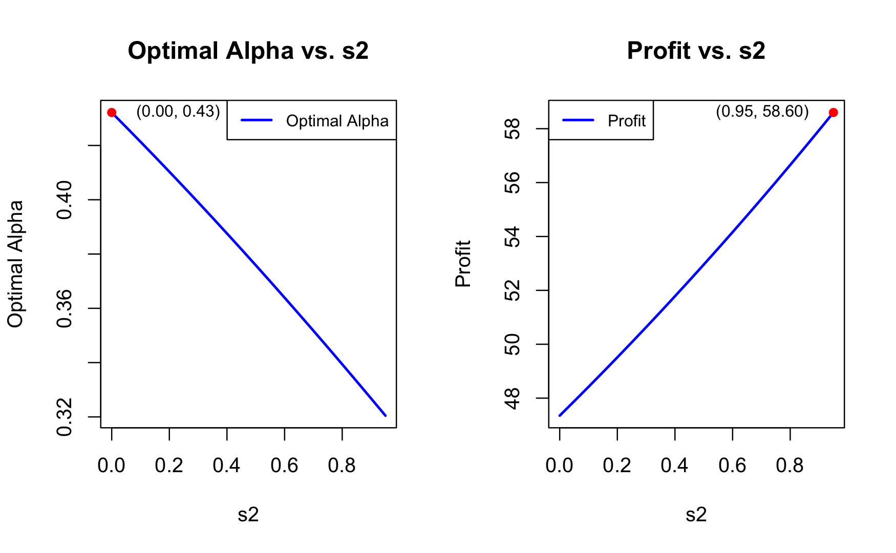
Figure 10: Optimal Level of Alpha and Profit Graph w.r.t. $s_{2}$

Policy Recommendations for Effective Low-Carbon Transitions

Encouraging effective low-carbon transitions requires a sensitive balance between assertive tax policies and a more targeted, limited subsidy approach. The above numerical analysis suggests several important and practical policy recommendations. While subsidies boost short-term profitability, they do not appear to incentivize long-term investment in low-carbon technologies adequately. This is evident from the decreasing trend in the optimal investment ratio ($\alpha$) as subsidy probabilities increase. On the other hand, higher emissions taxes consistently drive higher values of $\alpha$, indicating that tax policies play a more effective role in promoting robust investments in sustainable technologies.

- Expanding on Tax Strategies: A more structured and progressive carbon tax regime could enhance low-carbon transitions more effectively. By gradually increasing the cost of higher emissions, such a policy would not only penalize environmentally harmful practices but also provide businesses with the level of predictability they need in order to plan long-term investments in sustainability. This tax strategy could be further refined by introducing tax incentives for specific technologies that deliver substantial carbon reductions. For businesses, the clear financial penalties for high emissions and rewards for investing in sustainable solutions would create a strong motivation to prioritize clean technology adoption, ensuring a smoother and more predictable transition.

- Reassessing Subsidy Schemes: A more passive and targeted approach to subsidies is recommended. Direct financial incentives should be limited to sectors of the economy where low-carbon alternatives are not yet economically viable or where early-stage technologies need support to scale. This approach minimizes the risk of companies relying on subsidies for profitability without making a genuine progress toward sustainability. It also encourages firms to seek out real, long-term solutions rather than temporary financial relief. Companies should anticipate stricter regulatory standards in the future and take a proactive approach to sustainability. Rather than depending on subsidies alone, businesses are advised to prioritize investments in scalable, low-carbon technologies that align with long-term industry trends. Building internal capabilities for sustainable practices and integrating environmental risk assessments into financial planning can help ensure resilience against future regulatory shifts. Additionally, companies should explore partnerships with other industry players or research institutions to advance low-carbon innovations, as these collaborations can reduce costs and accelerate progress toward sustainability goals.

In summary, integrating fiscal policies, such as carbon taxes and subsidies, with broader regulatory measures can amplify their effectiveness with respect to promoting long-term sustainability and reducing emissions. For instance, mandatory carbon emission disclosures and stricter compliance requirements would not only improve transparency but also make tax and subsidy regimes more impactful. Businesses would be incentivized to adopt greener practices both to avoid penalties and to benefit from tax reliefs. This would create a feedback loop where fiscal and regulatory measures reinforce each other, driving a greater amount of corporate investments in sustainability.

Additionally, corporate leaders should adopt a forward-thinking approach, moving beyond short-term financial benefits emanating from current subsidies and tax reliefs. Strategic investments in low-carbon technologies today will prepare businesses for future regulatory shifts, reducing the risk of compliance costs down the line. Companies should conduct detailed cost-benefit analyses that balance immediate economic advantages with future regulatory expectations. Proactively enhancing sustainability measures will not only align businesses with global environmental trends but also provide a competitive edge in an increasingly eco-conscious market. This approach places companies in a better position against stricter regulations in the future and boosts their appeal to environmentally aware consumers.

Finally, investors should closely monitor governmental shifts in environmental policies, as these will impact the profitability and strategic positioning of companies in their portfolios. There is a clear advantage in diversifying investments to include companies with strong environmental strategies or those investing heavily in green technologies. Firms that are better prepared for stringent environmental regulations are more likely to thrive, benefiting from enhanced market reputation and consumer loyalty. Additionally, investors have the potential to influence corporate behavior by advocating for stronger sustainability practices within the companies they support. Active stewardship not only aligns investments with broader environmental goals but also helps mitigate the risks associated with regulatory changes, securing long-term profitability while promoting global sustainability objectives.

3 Conclusions

This paper explores the dynamics of firm’s strategic investment decisions that support the transition to a low-carbon economy, focusing on the interplay between government policies and corporate strategies. It reveals how corporations adjust their investment strategies based on anticipated returns and environmental impacts, with a cautious approach prevailing in the absence of government incentives. The analysis highlights that, while long-term sustainability goals are beneficial, they may impose significant short-term financial burdens on companies. When government intervention, through subsidies and taxes, is introduced, corporate behavior shifts dramatically. The findings in this paper show that assertive tax policies on carbon emissions effectively drive firm’s investment in sustainable technologies, aligning corporate actions with environmental targets. However, while subsidies enhance short-term profitability of firms, they can lead to a greater reliance on government aid and do not necessarily promote sustained innovation in green technologies.

The study suggests a balanced policy approach—where taxes are used assertively to stimulate investment, and subsidies are applied selectively to avoid dependency. This would encourage corporations to take proactive steps toward sustainability, aligning with long-term environmental goals rather than relying solely on government incentives. For stakeholders, particularly investors, the research underscores the importance of identifying companies that are actively adapting to evolving fiscal and regulatory landscapes. These companies are better positioned to meet future regulatory demands and capitalize on the growing market emphasis on sustainability, offering better long-term returns.

Extending the analytical framework to a multi-period setting under different decarbonization scenarios further reveals how the optimal investment ratio ($\alpha$) evolves over time. While aggressive early decarbonization yields the highest short-term profits for the firm, slower approaches offer better long-term profitability due to the lower upfront costs. The analysis also shows that sustainable investment in low-carbon technologies is beneficial in the long run, particularly in scenarios involving gradual transitions. In conclusion, this study provides practical insights for policymakers and business leaders on how to promote investments in low-carbon technologies. By implementing a balanced mix of taxes and targeted subsidies, governments can effectively encourage corporate sustainability efforts.

While the numerical examples presented in this paper provide valuable insights into the dynamics of decarbonization strategies, there is a noticeably potential to extend the model into a more general framework that relies on abstract variables rather than specific parameter values. One direction for this generalization is to define the production function, cost structure, and investment dynamics in terms of general parameters (e.g., $f(\alpha,k)$ for production efficiency, $g(A)$ for asset allocation) without relying on the sigmoid function or fixed coefficients such as $\beta$ and $k$. By introducing generalized mathematical forms, the model could capture a wider variety of industry-specific or region-specific decarbonization scenarios, making it applicable to diverse contexts.

Another avenue for extension lies in relaxing some of the simplifying assumptions made in this paper. For example:

1. The framework could incorporate multi-factor production functions, such as CES, that allow for varying degrees of substitutability between capital and efficiency. This would provide more flexibility in modeling how firms adapt to changing technological and regulatory environments.

2. Introducing uncertainty variables to account for fluctuations in energy prices, regulatory costs, or technological advancements could make the framework more robust to real-world complexities.

3. Expanding the time horizon to include dynamic decision-making models would allow firms to adjust their investment strategies iteratively in response to external changes.

4. Making a transition from a partial equilibrium framework to a general equilibrium framework to capture first-order welfare effects that are important for drawing policy recommendations.

Finally, transitioning to a more generalized theoretical framework would facilitate the development of closed-form solutions or approximate analytical results for key metrics, such as optimal investment ratios or profit trajectories, under a range of assumptions. This would reduce reliance on numerical simulations while retaining the core insights of the model. These extensions would not only enhance the versatility of the framework but also deepen its relevance for policymakers, firms, and researchers exploring sustainable transitions in diverse industries.

References

- AG (2019) AG, S., 2019. Siemens sustainability report 2019. URL: https://new.siemens.com/global/en/company/sustainability/reporting.html.
- Agency (2022) Agency, I.E., 2022. World Energy Outlook 2022. IEA. URL: https://www.iea.org/reports/world-energy-outlook-2022.
- Amazon (2020) Amazon, 2020. Amazon sustainability report. URL: https://sustainability.aboutamazon.com/. accessed: 2024-09-20.
- Bank of England (2018) Bank of England, 2018. Transition in thinking: The impact of climate change on the uk banking sector.
- Boyd (2013) Boyd, W., 2013. Public utility and the low-carbon future. UCLA L. Rev. 61, 1614.
- Carney (2015) Carney, M., 2015. Breaking the tragedy of the horizon–climate change and financial stability. Speech given at Lloyd’s of London 29, 220–230.
- Change et al. (2014) Change, I.C., et al., 2014. Mitigation of climate change. Contribution of working group III to the fifth assessment report of the intergovernmental panel on climate change 1454, 147.
- Cisagara (2024) Cisagara, B., 2024. Finance and climate change: assessing the impact of physical, transition, and regulation risks on asset pricing valuation. Journal of Asset Management , 1–23.
- Dietz et al. (2020) Dietz, S., Byrne, R., Gardiner, D., Gostlow, G., Jahn, V., Nachmany, M., Sullivan, R., 2020. Tpi state of transition report 2020. Transition Pathway Initiatives .
- Eccles et al. (2014) Eccles, R.G., Ioannou, I., Serafeim, G., 2014. The impact of corporate sustainability on organizational processes and performance. Management Science 60, 2835–2857.
- Fang et al. (2019) Fang, M., Tan, K.S., Wirjanto, T.S., 2019. Sustainable portfolio management under climate change. Journal of Sustainable Finance & Investment 9, 45–67.
- Holden et al. (2018) Holden, P.B., Edwards, N.R., Ridgwell, A., Wilkinson, R., Fraedrich, K., Lunkeit, F., Pollitt, H., Mercure, J.F., Salas, P., Lam, A., et al., 2018. Climate–carbon cycle uncertainties and the paris agreement. Nature Climate Change 8, 609–613.
- IKEA (2020) IKEA, 2020. Ikea sustainability report fy20. URL: https://about.ikea.com/en/sustainability. accessed: 2024-09-20.
- Institute (2015) Institute, W.R., 2015. Greenhouse Gas Protocol: A Corporate Accounting and Reporting Standard. World Resources Institute. URL: https://www.wri.org/publication/greenhouse-gas-protocol-corporate-accounting-and-reporting-standard.
- IPCC (2018) IPCC, 2018. Global Warming of 1.5°C. An IPCC Special Report on the impacts of global warming of 1.5°C above pre-industrial levels. Intergovernmental Panel on Climate Change. URL: https://www.ipcc.ch/sr15/.
- IPCC (2022) IPCC, 2022. Sixth Assessment Report (AR6), Working Group III: Climate Change 2022: Mitigation of Climate Change. Intergovernmental Panel on Climate Change. URL: https://www.ipcc.ch/report/ar6/wg3/.
- IPCC (2023) IPCC, 2023. Sixth Assessment Report (AR6) Synthesis Report: Climate Change 2023. Intergovernmental Panel on Climate Change. URL: https://www.ipcc.ch/report/ar6/syr/.
- Kober et al. (2020) Kober, T., Schiffer, H.W., Densing, M., Panos, E., 2020. Global energy perspectives to 2060–wec’s world energy scenarios 2019. Energy Strategy Reviews 31, 100523.
- Lenton et al. (2008) Lenton, T.M., Held, H., Kriegler, E., Hall, J.W., Lucht, W., Rahmstorf, S., Schellnhuber, H.J., 2008. Tipping elements in the earth’s climate system. Proceedings of the national Academy of Sciences 105, 1786–1793.
- McKinsey (2021) McKinsey, 2021. The net-zero transition: Its cost and benefits.
- NGFS (2019) NGFS, A., 2019. A call for action: Climate change as a source of financial risk. Network for Greening the Financial System: London, UK .
- Schulte and Hallstedt (2018) Schulte, J., Hallstedt, S.I., 2018. Company risk management in light of the sustainability transition. Sustainability 10, 4137.
- Semieniuk et al. (2021) Semieniuk, G., Campiglio, E., Mercure, J.F., Volz, U., Edwards, N.R., 2021. Low-carbon transition risks for finance. Wiley Interdisciplinary Reviews: Climate Change 12, e678.
- Siddique and Sultana (2018) Siddique, F.B., Sultana, I., 2018. Unilever sustainable living plan: A critical analysis. Global Journal of Management and Business Research 18.
- Tyfield (2013) Tyfield, D., 2013. Transportation and low carbon development, in: Low Carbon Development. Routledge, pp. 188–201.
- van Veelen (2021) van Veelen, B., 2021. Cash cows? assembling low-carbon agriculture through green finance. Geoforum 118, 130–139.
- Weng et al. (2015) Weng, H.H., Chen, J.S., Chen, P.C., 2015. Effects of green innovation on environmental and corporate performance: A stakeholder perspective. Sustainability 7, 4997–5026.