Estimating Discrete Choice Demand Models with Sparse Market-Product Shocks

Abstract

We propose a new approach to estimating the random coefficient logit demand model for differentiated products when the vector of market-product level shocks is sparse. Assuming sparsity, we establish nonparametric identification of the distribution of random coefficients and demand shocks under mild conditions. Then we develop a Bayesian procedure, which exploits the sparsity structure using shrinkage priors, to conduct inference about the model parameters and counterfactual quantities. Comparing to the standard BLP (Berry, Levinsohn  Pakes, 1995) method, our approach does not require demand inversion or instrumental variables (IVs), thus provides a compelling alternative when IVs are not available or their validity is questionable. Monte Carlo simulations validate our theoretical findings and demonstrate the effectiveness of our approach, while empirical applications reveal evidence of sparse demand shocks in well-known datasets.

Keywords: Demand Estimation, Sparsity, Bayesian Inference, Shrinkage Prior

JEL Codes: C1, C3, L00, D1

1 Introduction

Since Daniel L. McFadden’s seminal work (McFadden, 2001), the discrete choice model has become a basic tool for understanding consumer demand for differentiated products in many empirical context. As an important advancement of the literature, the BLP framework (Berry, 1994; Berry, Levinsohn  Pakes, 1995) allows researchers to estimate a flexible demand model that incorporates consumer preference heterogeneity and addresses price endogeneity, using aggregate (i.e., market-product level) data on price, quantity and other variables.

A prominent feature of the BLP framework is the inclusion of market-product-level demand shocks (a.k.a. unobserved market-product characteristics), which are observed by economic agents but not by econometricians. The dependence of price (or other endogenous variables) on these demand shocks provides a natural way to model the price endogeneity problem. However, this modeling strategy introduces a challenging estimation problem for two main reasons: (1) demand shocks enter the demand system nonlinearly, and (2) a dimensionality problem arises, as the number of parameters to estimate (including the demand shocks) exceeds the number of equations in the demand system. To address these challenges, BLP proposes inverting the demand system to recover the demand shocks, which are then interacted with a set of instrumental variables (IVs) to construct moment conditions for GMM estimation.

As emphasized by Berry  Haile (2014), the identification and estimation of the BLP model heavily depend on the availability of valid instrumental variables (IVs). In practice, finding suitable IVs for a specific empirical application is often challenging and requires consideration of data structure and availability, economic theory, institutional knowledge, and other contextual factors. Consequently, the literature has proposed and employed a wide range of IVs, including cost shifters (Berry, Levinsohn  Pakes, 19991; Goldberg  Verboven, 2001), BLP IVs (Berry, Levinsohn  Pakes, 1995), Hausman IVs (Hausman, 1994; Nevo, 2001), optimal IVs (Berry, Levinsohn  Pakes, 19991; Reynaert  Verboven, 2014), differential IVs (Gandhi  Houde, 2019), and time-series or panel data-based IVs (Sweeting, 2013; Jin, Lu, Zhou  Fang, 2021), among others. However, even with this variety of alternatives, practitioners often face difficulties in selecting appropriate IVs, especially when estimation results are highly sensitive to the choice of IVs. This sensitivity may arise from the weak IV problem, a common concern in empirical research that can also emerge theoretically under specific model assumptions (Armstrong, 2016).

In this paper, we propose an alternative approach to estimating the BLP model that eliminates the need for instrumental variables (IVs) by leveraging a sparsity assumption on market-product-level demand shocks. Specifically, we assume that in some markets, the demand shocks for certain products take the same market-specific value. Under this assumption and regularity conditions, we demonstrate that the demand shocks (including their sparsity structure) can be identified as model parameters, alongside other parameters characterizing consumer preferences in the random coefficients logit demand model. The sparsity assumption reduces the number of unknown parameters, enabling identification directly from the constraints in the model without relying on IV-based restrictions.

Our identification strategy, based on the sparsity assumption, naturally leads to a likelihood-based inference framework, in contrast to the traditional BLP method, which relies on demand inversion and IV-based moment conditions. For inference, we develop a Bayesian shrinkage approach that incorporates the sparsity assumption to estimate model parameters, including the sparsity structure, as well as counterfactual quantities such as price elasticities.

To handle the potentially very high-dimensional space of sparsity patterns for the market-product demand shocks, we employ a type of shrinkage priors, a variable selection technique in Bayesian statistics. Shrinkage priors have their roots in high-dimensional statistics and machine learning literature, and are connected to penalized likelihood estimators such as LASSO (Tibshirani, 1996) in the sense that the posterior modes can be considered equivalent to these estimators (Casella ., 2010). Shrinkage priors have been used successfully in linear econometric models such as VARs (e.g. Giannone ., 2021); see e.g. Korobilis  Shimizu (2022) for a review of shrinkage priors and their applications to linear models in economics. However, their application to non-linear models has been limited, probably due to the lack of theoretical understanding on how introducing sparsity can aid in the identification of parameters in these models. We bridge this gap by first studying how sparsity helps identification, which then motivates the use of shrinkage priors in our approach.

The proposed approach is both conceptually (returning to the likelihood framework for classic multinomial choice models) and computationally (offering a one-stop estimator for both preference parameters and the sparsity structure of demand shocks) straightforward. As such, it provides a compelling alternative to the BLP estimator, particularly when valid IVs are difficult to find or when researchers wish to evaluate the robustness of specific IV choices.

Monte Carlo simulation results show that, when the sparsity assumption holds in the data generating process (DGP), our approach performs similarly to the BLP estimator with strong IVs and outperforms the BLP estimator with potentially weak IVs. This supports our theoretical results on identification. Additionally, we examine cases where the demand shocks are not strictly sparse but exhibit approximate sparsity in the DGP, and find that our Bayesian shrinkage estimator still performs reasonably well in estimating the preference parameters, demonstrating robustness to mild misspecifications.

Depending on the empirical context, the sparsity assumption can have natural interpretations. For example, in supermarket scanner data applications where markets are defined by “store-week” pairs, the demand shocks may reflect unobserved promotion efforts at the store-week level for different products, usually identified by UPCs (Universal Product Code), after controlling for more aggregate fixed effects, such as brand, city, or quarter. In such cases, a store can only promote a selected subset of products in a given week due to limited shelf space (e.g., end-of-aisle displays), so the demand shocks for other products in the store-week will share the same value (either zero or the store-week level effect). Similarly, in Berry, Levinsohn  Pakes (1995)’s automotive market application, the demand shocks largely capture unobservable advertising efforts, which can vary across brands and models in different markets. Some brands or models may engage in active advertising campaigns in a specific market, while others may choose to maintain a more “standard level” of marketing effort.

We explore these interpretations by applying our approach to two empirical applications. First, we apply it to a supermarket scanner dataset, focusing on the yogurt category. In this case, we interpret the demand shocks as unobserved store-week-level promotion efforts. Our results demonstrate that the approach effectively captures the sparsity in promotion patterns across products, revealing important insights into consumer demand and store-level marketing strategies. Second, we revisit the automotive market data from Berry, Levinsohn  Pakes (1995), where we treat advertising efforts as unobserved demand shocks. We explore how these advertising efforts vary across brands and models in different markets. Both applications demonstrate the flexibility of our approach in capturing sparsity in demand shocks, offering a robust alternative to traditional IV-based methods.

1.1 Related Literature

Our identification result is related to several findings in the literature on the identification of random coefficients in BLP and/or classic multinomial choice models, including, among others, Fox, il Kim, Ryan  Bajari (2012), Fox  Gandhi (2016), Lu, Shi  Tao (2023), and Dunker, Hoderlein  Kaido (2023). While these results are developed under different assumptions and with distinct arguments, they are not directly applicable to our setting, where the $\xi$’s are sparse and both the number of products and markets are growing.

Moon . (2018) propose an approach to estimating the BLP model by modeling demand shocks as interactive fixed effects. While our paper shares a similar spirit of imposing structure on demand shocks, our identification and estimation strategies are fundamentally different. Their identification relies on additional exogenous variables and moment conditions, whereas ours depends solely on the sparsity condition described earlier. Moreover, their estimation strategy builds on least squares and minimum distance methods, while ours employs a Bayesian shrinkage approach. A related work by Gillen . (2019) introduces a LASSO-type estimator to select from a large number of control variables in the BLP model. In contrast, our focus is on addressing the challenge of high-dimensional demand shocks. Moreover, our estimation strategy differs significantly: their approach involves multiple steps of variable selection and requires post-selection inference, whereas ours is a Bayesian approach that delivers all results in a single pass.

Previous papers have proposed Bayesian estimation procedures of demand models for aggregate data. The approach introduced by R. Jiang . (2009) can be seen as a “Bayesian BLP,” where the likelihood is constructed via demand inversion. Our approach differs in that, while they treat the market-product shocks as econometric residuals as in BLP, we treat them as parameters. As a result, our method does not require demand inversion and is more scalable with respect to the number of products and markets, unlike R. Jiang . (2009), which requires demand inversion at each MCMC iteration.

In contrast to this, other Bayesian approaches, such as those by Yang . (2003) and Musalem . (2009), construct the likelihood by assigning an artificial set of consumer choices proportionally to the market shares. While this facilitates the estimation of the multinomial logit model for individual demand and the simulation of random coefficients, the sampling noise introduced at the data creation stage can potentially affect inference. Our approach avoids this issue by not requiring artificially assigned choices. Furthermore, as pointed out by Berry (2003), methods that assign artificial choices often lack a thorough discussion of identification and its relationship to prior restrictions. In contrast, our approach establishes a tight connection between identification under sparsity and estimation using shrinkage priors as a practical tool, effectively putting the identification argument into action.

Lastly, since our approach attempts to explore a large dimensional space of sparsity pattern of the market-product shocks, broadly speaking, this paper also contributes to the expanding literature on high-dimensional demand estimation: (Chiong  Shum, 2019: random projection for aggregate demand model with many products, Smith  Allenby, 2019: random partitions of products, Loaiza-Maya  Nibbering, 2022: high-dimensional probit models, Z. Jiang ., 2024: graphical lasso for flexible substitution patterns, Iaria  Wang, 2024: model of demand for bundles, Ershov ., 2024: estimation of complementarity with many products, Chib  Shimizu, 2024: scalable estimation of consideration set models).

The rest of the paper is organized as follows. Section 2 introduces a sparsity condition and establishes the identification of the model. Section 3 proposes a shrinkage-prior-based Bayesian estimation method. Section 4 investigates the performance of the proposed approach through Monte Carlo simulations. Section 5 applies the proposed approach to two well-known real datasets and finds empirical evidence of sparsity in both. Section 6 concludes.

2 Model and Identification

2.1 Model

We consider a stylized random coefficient logit demand model for aggregate data, in the spirit of Berry, Levinsohn  Pakes (1995). There are $T$ markets, indexed by $t=1,\dots,T$, each consisting of $J_{t}+1$ products, indexed by $j=0,1,\dots,J_{t}$, and $N_{t}$ consumers, indexed by $i=1,\dots,N_{t}$. The products indexed by $j>0$ are “inside goods,” and product $0$ is the “outside option.”

Each consumer $i$’s utility from product $j$ in market $t$ is given by

$$u_{ijt}=X_{jt}^{\top}\beta_{i}+\xi_{jt}+\varepsilon_{ijt},$$ (1)

where $X_{jt}\in\mathbb{R}^{d_{X}}$ is a vector of observed market-product characteristics, $\beta_{i}$ represents consumer-specific taste parameters (i.e., random coefficients), which are i.i.d. across consumers and follow the distribution $f\in\mathcal{F}$, $\xi_{jt}$ is the market-product level demand shock (a.k.a. unobserved characteristic), and $\varepsilon_{ijt}$ is an i.i.d. idiosyncratic preference shock across $i$, $j$, and $t$, following the standard Gumbel distribution. To normalize the level of the random utility, the product characteristics and demand shock of the outside option, $X_{0t},\xi_{0t}$, are set to zero.

As is typical in aggregate demand modeling, we allow certain variables in $X_{jt}$, such as price, to be endogenous. This endogeneity arises because these variables may depend on $\xi_{jt}$, which the firm can observe when setting prices or making other decisions, but econometricians cannot. We do not specify a detailed supply-side model for this dependence but will return to it later when discussing the identification assumptions.

In each market $t$, each consumer chooses the product that maximizes their utility, and aggregating consumer choices gives the market share of each product $j$ as follows:

$$\sigma_{jt}\left(\xi_{t},f\right)=\int\frac{\exp\left(X_{jt}^{\top}\beta+\xi_{jt}\right)}{1+\sum_{k=1}^{J_{t}}\exp\left(X_{kt}^{\top}\beta+\xi_{kt}\right)}f(\beta)\,d\beta,$$ (2)

where $\xi_{t}=(\xi_{1t},\dots,\xi_{J_{t}t})^{\top}$. Note that our setup encompasses the typical specification in most empirical applications, where some coefficients in $X_{jt}$ are fixed (i.e., these random coefficients follow degenerate distributions). We will consider these special cases in the Monte Carlo simulations and empirical applications.

The observed market share of product $j$ in market $t$ is $s_{jt}=\frac{\sum_{i=1}^{N_{t}}y_{ijt}}{N_{t}}$, where $y_{ijt}$ is an indicator that equals to 1 if $i$ chooses product $j$ in market $t$ and 0 otherwise. By definition, the market share vector $\left(s_{0t},...,s_{J_{t}t}\right)\in\Delta^{J_{t}}$, where $\Delta^{J_{t}}$ is the standard $J_{t}$-simplex. The likelihood function of the observed choices is

$$L\left(f,\xi_{1},...,\xi_{T}\right)=\prod_{t=1}^{T}\prod_{i=1}^{N_{t}}\prod_{j=0}^{J_{t}}\left[\sigma_{jt}\left(\xi_{t},f\right)\right]^{y_{ijt}}=\prod_{t=1}^{T}\prod_{j=0}^{J_{t}}\left[\sigma_{jt}\left(\xi_{t},f\right)\right]^{q_{jt}},$$ (3)

where $q_{jt}=\sum_{i=1}^{N_{t}}y_{ijt}$ is the total quantity of product $j$ in market $t$. The aggregation across consumers (second equality) is due to the fact that the aggregate data do not contain individual-level attributes, e.g., demographics. When individual-level data are available, our approach can be modified easily to incorporate this information (such an extension is available upon request).

Without additional restrictions, estimating $\left(f,\xi_{1},...,\xi_{T}\right)$ based on the likelihood function (3) is infeasible, as there are only $\sum_{t=1}^{T}J_{t}$ linearly independent first-order conditions while the number of unknown parameters is $\sum_{t=1}^{T}J_{t}+\dim\left(f\right)$, where $\dim\left(f\right)$ denotes the dimensionality of $f$. In particular, these conditions effectively constitute the demand system

$$s_{jt}=\sigma_{jt}\left(\xi_{t},f\right)\>\forall j,t,$$ (4)

and it is evident that the system is underidentified.

In the following, we first review the standard BLP approach to addressing this dimensionality problem and then introduce our new strategy to resolve it.

2.2 The BLP Approach

The standard BLP approach to addressing the identification problem consists of two main components. First, for a given $f$, the demand system in (4) is inverted (invertibility is established in Berry (1994) and Berry, Gandhi  Haile (2013)) to obtain:

$$\xi_{jt}=\sigma_{jt}^{-1}(s_{t},f),\quad\forall j,t.$$ (5)

Next, the $\xi_{jt}$’s are treated as econometric residuals, satisfying the following conditional moment restrictions:

$$E\left[\xi_{jt}\mid Z_{jt}\right]=E\left[\sigma_{jt}^{-1}(s_{t},f)\mid Z_{jt}\right]=0,\quad\forall j,t,$$ (6)

where $Z_{jt}$ is a vector of instrumental variables (IVs). If the IVs provide sufficient variation, then the distribution $f$ is identified and can be estimated via GMM.

Since there are endogenous product characteristics, such as price, and market shares in the moment conditions, the IVs $Z_{jt}$ must include exogenous variables that are excluded from $X_{jt}$ (see Berry  Haile (2014)). A practical challenge in empirical applications is that it can be difficult to identify and/or construct valid IVs for implementing the BLP GMM estimator. While this issue has been extensively discussed in the literature, there is still significant debate about how best to address it. Notable works on the subject include, among others, Berry, Levinsohn  Pakes (1995), Berry, Levinsohn  Pakes (19992), Reynaert  Verboven (2014), Armstrong (2016), and Gandhi  Houde (2019).

2.3 Sparsity Assumption on Demand Shocks

We propose an alternative approach to the identification problem based on the demand system (4). Instead of imposing conditional moment restrictions (or other distributional assumptions) on $\xi_{jt}$’s, like (6), we treat $\xi_{t}$’s as parameters to be estimated and assume they exhibit a sparsity structure: for some market $t$, a sub-vector of $\xi_{t}$ shares the same value, as formally stated in Assumption 1.

Assumption 1 (Sparsity).

There exist a set of markets $\mathcal{S}\subset\left\{1,...,T\right\}$ and a set of products $\mathcal{K}_{t}\subset\left\{1,...,J_{t}\right\}$ for each $t\in\mathcal{S}$, such that $\xi_{jt}=\xi_{kt}$ for any $j,k\in\mathcal{K}_{t}$. Furthermore, $\left|\mathcal{S}\right|\rightarrow\infty$ and $\left|\mathcal{K}_{t}\right|\rightarrow\infty$ for each $t\in\mathcal{S}$.

Assumption 1 basically says that for any market $t\in\mathcal{S}$, all the $\xi_{jt}$’s for $j\in\mathcal{K}_{t}$ have the same value, which is denoted as $\nu_{t}\in\mathbf{R}$. So the number of unknowns in $\xi_{t}$ is reduced by $\left|\mathcal{K}_{t}\right|-1$ (from $J_{t}$), which in turn implies that the number of unknowns in the demand system (4) decreases by $\sum_{t\in\mathcal{S}}\left(\left|\mathcal{K}_{t}\right|-1\right)$. Intuitively, the reduction in the number of unknown parameters can circumvent the dimensionality problem and restore the identification of $\left(f,\xi_{1},...,\xi_{T}\right)$.

To ensure that there is a sufficient reduction in the number of parameters, Assumption 1 further requires that: 1) in a market with sparse $\xi_{t}$, the number of products with the same value of $\xi_{jt}$ goes to infinity as $J_{t}\rightarrow\infty$; 2) the number of such markets (with sparse $\xi_{t}$’s) goes to infinity as $T\rightarrow\infty$. Theses requirements are necessary for the nonparametric identification of $\left(f,\xi_{1},...,\xi_{T}\right)$, which can be relaxed if $\dim\left(f\right)$ is finite due to parametric restrictions, e.g., Gaussian distribution.

Assumption 1 has important implications for the canonical price (and/or other product characteristics) endogeneity problem. To see this, let us consider a concrete example.

Example 1.

Suppose one element of $X_{jt}$ is price $P_{jt}$ and it is determined by a linear function

$$P_{jt}=Z_{jt}^{\top}\rho+\xi_{jt},$$

where $Z_{jt}$ is the vector of IVs and $\rho$ is a vector of parameters. Also, for any market $t$, $\xi_{jt}$ is generated as

$$\xi_{jt}=\begin{cases}\nu_{t},&\text{with prob }\varphi\\ \xi_{jt}^{*},&\text{with prob }1-\varphi,\end{cases}$$

where $\nu_{t}$ and $\xi_{jt}^{*}$ are two mean-zero random variables that are independent of each other. So the probability $\varphi$ captures the degree of sparsity in $\xi$’s.

In this case, the price endogeneity problem can be measured by the conditional (given $Z_{t}$) covariance of $P_{jt}$ and $\xi_{jt}$. Suppressing the conditioning variables $Z_{t}$ for notational simplicity, we have

$$\text{Cov}\left(P_{jt},\xi_{jt}\right)=\text{Var}\left(\xi_{jt}\right)=E\left(\xi_{jt}^{2}\right)=\varphi\text{Var}\left(\nu_{t}\right)+\left(1-\varphi\right)\text{Var}\left(\xi_{jt}^{*}\right).$$ (7)

When $\varphi$ is small, i.e., not much sparsity in $\xi$’s, the second term in (7) dominates so price endogeneity is captured by the variance of $\xi_{jt}^{*}$. As $\varphi$ gets larger, i.e., more sparsity in $\xi$’s, the variance of $\nu_{t}$ becomes more important in determining the severity of the endogeneity problem. Thus, if the across market variation of $\nu_{t}$ is small comparing to the across market-product variation of $\xi_{jt}^{*}$, then more sparsity implies less endogeneity. Of course, the converse is also true. To sum up, the sparsity assumption has certain implications on the price endogeneity problem, but does not necessarily reduce its severity.

In general, the sparsity assumption is neither stronger or weaker than the conditional mean restriction (6). The assumption (6) does not restrict the form of price endogeneity; however, it requires valid IVs. On the contrary, the sparsity assumption imposes certain restrictions on the form of price endogeneity; however, it avoids the need for IVs completely.

One particularly interesting feature of the sparsity assumption is that it does not impose any restrictions on the $\xi_{jt}$’s in the non-sparse set. In particular, these $\xi_{jt}$’s can either be realizations of any continuous or discrete distributions. Also, they can arbitrarily depend on $X_{jt}$ and $Z_{jt}$ (these IVs are not valid in this case). On the contrary, typical statistical assumptions on $\xi_{jt}$’s, such as (6) or other distributional assumptions, imply much stronger restrictions on the non-sparse set.

Next, we shall explore how Assumption 1 can help identify the model. The next subsection will establish the main identification result that shows that both $\xi_{t}$’s and $f$ are identified by the demand system (4) under the sparsity assumption and some other conditions. Before diving into the formal result, it is instructive to illustrate its key idea via a nested-logit example.

Example 2 (Nested-Logit with Sparse $\xi$).

Consider a nested-logit model (as in Berry (1994)) of consumer demand for 4 inside goods and an outside option. For convenience, we focus on a single market and omit the subscript $t$. The products are grouped into mutually exclusive nests, with the outside option $0$ being the only member in its own nest. The utility function of consumer $i$ can be written as

$$u_{ij}=\begin{cases}\beta X_{j}+\xi_{j}+\zeta_{ig(j)}+\left(1-\lambda\right)\epsilon_{ij},&j=1,2,3,4\\ \zeta_{i0}+\left(1-\lambda\right)\epsilon_{i0},&j=0,\end{cases}$$

where $X_{j}\in\textbf{R}$ is an observed product characteristic, $\zeta_{ig(j)}$ is a random coefficient following a specific distribution (Cardell, 1997), $g(j)$ labels the nest of product $j$, $\lambda$ is the “nesting parameter” and $\epsilon_{ij}$ is the “logit error” following the standard Gumbel distribution.

Suppose we know the sparsity pattern is $\xi_{2}=\xi_{3}=\xi_{4}=\nu$. Then the parameters to be identified are $\beta,\lambda,\xi_{1},\nu$. Given the close-form inversion of nested-logit model, we obtain the following linear system

$$\xi_{1}+\beta X_{1}+\lambda\log\left(\bar{s}_{1|g(1)}\right) =\log\left(\frac{s_{1}}{s_{0}}\right)$$

$$\nu+\beta X_{2}+\lambda\log\left(\bar{s}_{2|g(2)}\right) =\log\left(\frac{s_{2}}{s_{0}}\right)$$

$$\nu+\beta X_{3}+\lambda\log\left(\bar{s}_{3|g(3)}\right) =\log\left(\frac{s_{3}}{s_{0}}\right)$$

$$\nu+\beta X_{4}+\lambda\log\left(\bar{s}_{4|g(4)}\right) =\log\left(\frac{s_{4}}{s_{0}}\right),$$

where $s_{j}$ is the market share of product $j$ and $\bar{s}_{j|g(j)}$ denotes the within-group share of product $j$ in its nest $g(j)$.

There are 4 equations and 4 unknowns, so the parameters are determined by

$$\begin{pmatrix}\xi_{1}\\ \nu\\ \beta\\ \lambda\end{pmatrix}=\begin{bmatrix}1&0&X_{1}&\log\left(\bar{s}_{1|g(1)}\right)\\ 0&1&X_{2}&\log\left(\bar{s}_{2|g(2)}\right)\\ 0&1&X_{3}&\log\left(\bar{s}_{3|g(3)}\right)\\ 0&1&X_{4}&\log\left(\bar{s}_{4|g(4)}\right)\end{bmatrix}^{-1}\begin{bmatrix}\log\left(\frac{s_{1}}{s_{0}}\right)\\ \log\left(\frac{s_{2}}{s_{0}}\right)\\ \log\left(\frac{s_{3}}{s_{0}}\right)\\ \log\left(\frac{s_{4}}{s_{0}}\right)\end{bmatrix}.$$ (8)

We can see that the identification condition in this special case boils down to the invertibility of the matrix in (8). The invertibility requires that the vector $X$ cannot be collinear with the indicator variables for the sparse set (the first two columns in the matrix), which automatically holds when $X$ is continuous.

This example highlights the key role of the sparsity assumption in identification: it reduces the number of unknown parameters from 6 ($\beta,\lambda$ and all the $\xi$’s) down to 4 so we have sufficient number of equations. Based on this insight, we can expect that, to identify a more complicated model with more parameters, we will need data on more products and/or markets, as well as a sufficient degree of sparsity. Also, the nested-logit model, which is a special case of the general random coefficient logit model (1), has a close-form inversion in $\xi$’s, so we can derive an explicit solution for the parameters. However, for the general model that does not have close-form inversion, establishing identification requires additional technical conditions and arguments.

2.4 Non-parametric Identification with Sparse Demand Shocks

In this subsection, we establish the formal non-parametric identification result, Theorem 1 under the sparsity assumption. Given Assumption 1, without loss of generality, suppose $\mathcal{K}_{t}=\left\{K_{t}+1,...,J_{t}\right\}$, i.e., the $\xi_{jt}$’s for the last $J_{t}-K_{t}$ products takes the same value $\nu_{t}$. Then for each market $t$, let

$$\Xi_{t}=\left\{\xi_{t}\in\mathbf{R}^{J_{t}}:\xi_{jt}=\nu_{t}\text{ for any }j\in\mathcal{K}_{t}\right\}$$

denote the space of $\xi_{t}$’s restricted by Assumption 1.

For a given $f\in\mathcal{F}$ and any market $t$, there are $K_{t}+1$ unknowns, $\left(\xi_{1t},...,\xi_{K_{t}t}\right)$ and $\nu_{t}$, and $J_{t}$ equations in the demand system (4). So intuitively we may only need the first $K_{t}+1$ equations, i.e,

$$s_{jt}=\sigma_{jt}\left(\xi_{t},f\right),\>j=1,...,K_{t}+1,$$ (9)

to solve for the vector $\left(\xi_{1t},...,\xi_{K_{t}t},\nu_{t}\right)$. Lemma 1 confirms that this is the case so the demand system (9), and hence (4), is invertible in $\xi_{t}\in\Xi_{t}$ for any $f\in\mathcal{F}$, which is a slight modification of the invertibility result in Berry (1994).

Lemma 1.

Suppose $s_{jt}>0$ for any $j,t$. Then for any $f\in\mathcal{F}$ and any $t$, there is a unique $\xi_{t}\in\Xi_{t}$ that satisfies the demand system $s_{jt}=\sigma_{jt}\left(\xi_{t},f\right),\>j=1,...,J_{t}$. Moreover, for any $t$, $\xi_{jt}=\tilde{\sigma}_{jt}^{-1}\left(\tilde{s}_{t},f\right)$ for any $j=1,...,K_{t}+1$, where $\tilde{s}_{t}=\left(s_{1t},...,s_{K_{t}+1,t}\right)$ and $\left[\tilde{\sigma}_{1t}^{-1}\left(\tilde{s}_{t},f\right),...,\tilde{\sigma}_{K_{t}+1,t}^{-1}\left(\tilde{s}_{t},f\right)\right]$ denotes the solution of the system (9).

Proof.

See Appendix A.1. ∎

Lemma 1 gives us the inversion of the subsystem (9), i.e., $\xi_{jt}=\tilde{\sigma}_{jt}^{-1}\left(\tilde{s}_{t},f\right)$, $j=1,...,K_{t}+1$. We can substitute these inverse demand functions into the last $J_{t}-K_{t}-1$ equations of (4) to obtain

$$s_{jt}=\sigma_{jt}\left(\tilde{\sigma}_{t}^{-1}\left(\tilde{s}_{t},f\right),f\right),\>j=K_{t}+2,...,J_{t},\forall t,$$ (10)

where $\tilde{\sigma}_{t}^{-1}\left(\tilde{s}_{t},f\right)=\left[\sigma_{1t}^{-1}\left(\tilde{s}_{t},f\right),...,\sigma_{K_{t}+1,t}^{-1}\left(\tilde{s}_{t},f\right)\right]^{\top}$. Note that the only unknown object in (10) is $f$, so the identification problem becomes whether $f$ is uniquely determined by (10). To establish identification, we need to introduce additional assumptions.

Assumption 2.

The random vector $X_{jt}$ is independent across $j,t$, and has continuous and full support in $\mathbf{R}^{d_{X}}$.

Assumption 2 rules out the cases where $X_{jt}$ has discrete or bounded support. This is not surprising if we want to identify a continuous $f$ nonparametrically. Similar continuous support assumptions are also imposed in related studies, see among others, the Assumption 2 of Fox . (2012) and the Assumption 7 of Lu . (2023). The continuous support assumption can be relaxed when a sub-vector of the coefficients on $X_{jt}$ are fixed and/or $f$ is parameterized by a finite number of parameters, as commonly estimated models in practice.

Also, Assumption 2 requires that $X_{jt}$ has full support, so that we can establish identification based on the “identification at infinity” argument, as in Lewbel (2000), Khan  Tamer (2009), among others.

Assumption 3.

For any $f\in\mathcal{F}$, $\sup_{x\in\mathcal{B}}\int\exp\left(x^{\top}\beta\right)f\left(\beta\right)d\beta<\infty$ for any bounded open $\mathbf{R}^{d_{X}}$-ball $\mathcal{B}$.

Assumption 3 is a regularity condition restricting the tail of $f$ to be exponential or subexponential, which is satisfied by Gaussian distributions, for example. This assumption is necessary for our identification argument based on the uniqueness of Laplace transform; it can be viewed as an alternative restriction on the shape of $f$ to the bounded support assumption imposed in Fox, il Kim, Ryan  Bajari (2012).

As we shall show in the proof of Theorem 1, Assumption 1, 2, and 3 imply that $f$ can be nonparametrically identified by the subsystem (10). Combining this result with Lemma 1, we can conclude that both $\xi_{jt}$’s and $f$ are identified by the demand system (4), as stated in Theorem 1.

Theorem 1.

If the conditions of Lemma 1, Assumptions 1, 2 and 3 hold, then $\xi_{t}\in\Xi_{t}$ for all $t=1,...,T$ and $f\in\mathcal{F}$ are identified by the demand system (4).

Proof.

See Appendix A.2. ∎

Remark 1.

Comparing with the canonical identification result for BLP in Berry  Haile (2014), which relies on demand inversion and IVs, Theorem 1 exploits the sparsity structure in $\xi$’s but does not require IVs. Note that demand inversion is still used in the proof of Theorem 1: we employ the inversion of the subsystem (9) to establish the identification of $\xi$’s for a given $f$. However, in our context, the inversion is only used as a theoretical device in the proof; as we shall see later, our estimation procedure does not require explicitly computing the demand inversion. This stands in contrast with the BLP estimation strategy, where demand inversion is computed repeatably in the estimation procedure.

3 Bayesian Shrinkage Approach to Estimation

The identification result established by Theorem 1 is conditional on the sparsity structure defined by $\Xi_{t}$’s. If the sparsity structure were known, then we could simply implement the MLE (using (3)) with restrictions on $\xi_{t}$’s defined by $\Xi_{t}$’s. However, in practice, we typically do not observe the sparsity structure ex-ante, just as the situation in the classical high-dimensional regression context with many predictors. In this section, we shall borrow insights from the high-dimensional Bayesian statistics literature to design an inference procedure that can both uncover the latent sparsity structure and deliver estimates of the parameters of interests.

The latent sparsity structure is a high-dimensional object comprised of the following components:

1. $\mathcal{S}\subset\{1,\ldots,T\}$, the set of “sparse” markets exhibiting sparsity in $\xi$’s;

2. $\mathcal{K}_{t}\subset\{1,\ldots,J_{t}\}$ for each $t\in\mathcal{S}$, the set of “sparse” products such that $\xi_{jt}=\nu_{t}$ for any $j\in\mathcal{K}_{t}$.

For each market $t\in\mathcal{S}$, there are essentially $2^{J_{t}}$ possible configurations of $\mathcal{K}_{t}$. Moreover, there are $2^{T}$ possible sets of sparse markets $\mathcal{S}$. For example, in the automobile market application of Berry, Levinsohn  Pakes (1995), there are 20 markets and on average 110 products in each market, indicating a very large dimensionality of the parameter space that we need to explore when estimating the model.

The problem of finding such sparsity structure is akin to the variable selection problem in high-dimensional linear regression with many predictors for which frequentist penalized likelihood methods such as LASSO (Tibshirani, 1996) and Bayesian shrinkage prior methods are widely used. In this paper, we propose a stochastic search method based on shrinkage priors for the ease of uncertainty quantification (Casella ., 2010, Womack ., 2014, Porwal  Raftery, 2022). For recent applications of shrinkage priors in econometrics, primarily on linear models, see e.g., Giannone, Lenza  Primiceri (2021), Koop  Korobilis (2023), and Smith  Griffin (2023). Our novel identification result in Theorem 1 motivates the use of shrinkage priors in the non-linear model considered in this paper.

Conceptually, ex-ante deviations of $\xi_{jt}$ are penalized or “shrunk” towards zero via a prior distribution that is centered around zero. In particular, we employ a type of spike-and-slab priors (Mitchell  Beauchamp, 1988, George  McCulloch, 1993, George  McCulloch, 1997, Ishwaran  Rao, 2005, Narisetty  He, 2014, Ročková  George, 2018) to shrink $\xi_{jt}$ towards zero. With the spike-and-slab priors, one can easily obtain probabilistic statement about sparsity (i.e. $\xi_{jt}=\nu_{t}$) in contrast to the penalized likelihood approaches which are based on constrained optimization problems.

3.1 The likelihood

We introduce our estimation procedure with a commonly used parametric specification of the distribution of random coefficients ($f$), for the ease of exposition. A non-parametric extension using sieve approximation, as in Lu, Shi  Tao (2023) and Wang (2023), is possible, given the general non-parametric identification result of Theorem 1, however, it is beyond the scope of the current paper so we leave it for future research.

Specifically, let the random coefficients follow an independent normal distribution:

$$\beta\sim N_{d_{X}}(\bar{\beta},\Sigma),$$

where $\Sigma=\text{diag}(\sigma^{2}_{1},\ldots,\sigma^{2}_{d_{X}})$. Again we assume independence for the ease of exposition, it is straightforward to include non-zero off diagonal elements in $\Sigma$. Note that this formulation nests the common case where only some of the $d_{X}$ covariates are assigned random coefficients. For example, with $d_{X}=3$ and if only the first variable has random coefficients, we have $\Sigma=\text{diag}(\sigma^{2}_{1},0,0)$.

For convenience, we re-parametrize the non-negative elements in $\Sigma$ as in R. Jiang, Manchanda  Rossi (2009). First, we decompose $\Sigma=RR^{\prime}$, where $R=\text{diag}(\sigma_{1},\ldots,\sigma_{d_{X}})$. Then let $r=(r_{1},\ldots,r_{d_{X}})^{\prime}$ be the log standard deviations of the random coefficients, i.e. $r_{k}=\log(\sigma_{k})$. Consequently, $R=\text{diag}(e^{r_{1}},\ldots,e^{r_{d_{X}}})$. Next, let $\xi_{jt}=\bar{\xi}_{t}+\eta_{jt}$, where $\bar{\xi}_{t}$ is a “common shock” to market $t$ and $\eta_{jt}$ is the market-product $(j,t)$- specific deviation from $\bar{\xi}_{t}$. Note that a sparse vector $\xi_{t}$ (as in Theorem 1) is a special case of this formulation: letting $\bar{\xi}_{t}=\nu_{t}$, so $\eta_{jt}=0$ if $j\in\mathcal{K}_{t}$ and $\eta_{jt}=\xi_{jt}-\nu_{t}$ otherwise.

Given the above parameterization, the utility function (1) can be re-written as

$$u_{ijt}=\delta_{jt}+\mu_{ijt}+\varepsilon_{ijt},$$

where $\delta_{jt}=X_{jt}^{\top}\bar{\beta}+\xi_{jt}$ and $\mu_{ijt}=X_{jt}^{\top}Rv_{i}$. The $d_{X}$-dimensional vector $v_{i}$ is i.i.d. and follows the product of $d_{X}$ independent standard normal distributions. Consequently, the predicted market share is

$$\sigma_{jt}\left(\xi_{t},\bar{\beta},r\right)=\int\frac{\exp\left(\delta_{jt}+\mu_{ijt}\right)}{1+\sum_{k=1}^{J_{t}}\exp\left(\delta_{kt}+\mu_{ikt}\right)}\phi\left(v_{i}|0,I\right)dv_{i},$$ (11)

where $\phi\left(\cdot|0,I\right)$ is the $d_{X}$-dimensional standard normal density. We approximate the integral based on $R_{0}$ i.i.d. draws of $v_{i}$ from the normal distribution. The likelihood is defined as

$$p\left(\bar{\beta},r,\bar{\xi}_{1},...,\bar{\xi}_{T},\eta_{1},\ldots,\eta_{T}|q\right)=\prod_{t=1}^{T}\prod_{j=0}^{J_{t}}\left[\sigma_{jt}\left(\xi_{t},\bar{\beta},r\right)\right]^{q_{jt}},$$ (12)

where $\eta_{t}=(\eta_{1t},\ldots,\eta_{J_{t}t})^{\top}$, $q=\{q_{1},\ldots,q_{T}\}$ and $q_{t}=(q_{1t},\ldots,q_{J_{t}t})^{\top}$.

Note that we could define $\bar{\xi}_{t}$’s as part of $\bar{\beta}$ by modifying the covariates appropriately, but especially when $T$ is large, it is computationally more efficient to separately update the market specific intercepts from the slopes. We therefore treat them separately in what follows.

3.2 Prior

The sparsity assumption (Assumption 1) is a key identifying restriction we exploit to estimate the model. Our Bayesian approach naturally incorporates the sparsity restriction via a spike-and-slab prior on $\eta_{jt}$’s. A practical advantage of this approach is that it provides a one-step inference procedure for both model parameters and the latent sparsity structure of $\xi$’s.

The (continuous) spike-and-slab prior (George  McCulloch, 1993, George  McCulloch, 1997) is a popular method for stochastic search variable selection. Other types of shrinkage priors can be also used in our framework, but the unique feature of the spike-and-slab type priors is the ease of interpretation of the estimated sparsity structure as we will see shortly.

Specifically, we define the prior on the unobserved market-product shocks as

$$\eta_{jt}\sim(1-\gamma_{jt})N(0,\tau^{2}_{0})+\gamma_{jt}N(0,\tau^{2}_{1}),$$ (13)

independently over $j$ and $t$, where $0<\tau^{2}_{0}\ll\tau^{2}_{1}$ are the prior variances in the two component mixture of normals with $\tau^{2}_{0}$ taking a very small value and $\tau^{2}_{1}$ a large value. The binary indicator $\gamma_{jt}$ equals to 0 if the $\eta_{jt}$ belongs to the “spike” component and $1$ if it is in the “slab” component. Intuitively, if $\gamma_{jt}=0$, $\eta_{jt}$ is shrunk toward zero (i.e. $\xi_{jt}$ is shrunk toward $\bar{\xi}_{t}$). On the other hand, when $\gamma_{jt}=1$, it is unrestricted (i.e. $\xi_{jt}$ deviates from $\bar{\xi}_{t}$). To be more precise, the posterior density on $\eta_{jt}$ is proportional to the likelihood times its prior. When it belongs to the spike component, the prior dominates, and virtually $\eta_{jt}$ is shrunk to zero in the posterior distribution. The posterior mean of $\gamma_{jt}$ will inform us the ex-post uncertainty of whether $\eta_{jt}$ is zero or not, i.e. $(jt)\in\mathcal{K}_{t}$ or not. Note that for each market $t$, the $J_{t}$-dimensional vector $\gamma_{t}=(\gamma_{1t},\ldots,\gamma_{J_{t}t})^{\prime}$ summarizes the $2^{J_{t}}$ possible sparsity patterns.

A priori, the binary variable $\gamma_{jt}$’s are i.i.d. and follow a Bernoulli distribution with the prior inclusion probability $\phi_{t}$ that is specific to market $t$ so to allow for different degrees of sparsity across markets $t=1,\ldots,T$:

$$\gamma_{jt}\overset{iid}{\sim}\text{Bernoulli}(\phi_{t}),\ j=1,\ldots,J_{t}.$$

We follow the convention and specify a beta prior on $\phi_{t}$:

$$\phi_{t}\overset{iid}{\sim}\text{Beta}(\underline{a}_{\phi},\underline{b}_{\phi}),\ t=1,\ldots,T.$$

Markets $(t)$ in the sparse set $\mathcal{S}$ are associated with small values of $\phi_{t}$, and market-product pairs $(jt)$ with $\gamma_{jt}=0$ are in the sparse product set $\mathcal{K}_{t}$. We set $(\underline{a}_{\phi},\underline{b}_{\phi})=(1,1)$ so that ex-ante, all the market-specific prior inclusion probability $\phi_{t}$ has mean of 0.5. In other words, the prior probability that each market-product shock $\eta_{jt}$ is sparse is 50%.

For the remaining parameters, we employ standard priors independently

$$\bar{\beta} \sim N_{d_{X}}(\underline{\mu}_{\beta},\underline{V}_{\beta}),$$

$$\bar{\xi}_{t} \overset{ind}{\sim}N(\underline{\mu}_{\xi_{t}},\underline{V}_{\xi_{t}}),\quad t=1,\ldots,T,$$

$$r_{k} \overset{ind}{\sim}N(0,\underline{V}_{r,k}),\quad k=1,\ldots,d_{X},$$

a $d_{X}$-dimensional normal prior for the slope vector $\bar{\beta}$, an normal prior for the market-specific product shock $\bar{\xi}_{t}$ independently over markets, and a normal prior for the log standard deviation of the random coefficients independently over covariates. We let $(\underline{\mu}_{\beta},\underline{V}_{\beta})=(0,10\cdot I_{d_{X}})$ and $(\underline{\mu}_{\xi_{t}},\underline{V}_{\xi_{t}})=(0,10)$ for all markets $t$ to give sufficiently uninformative priors on the fixed slope parameter $\bar{\beta}$ and the market specific shocks $\bar{\xi}_{t}$. For the log standard deviations, we let $\underline{V}_{r,k}=0.5$ for all $k$ to give sufficiently uninformative prior on $\Sigma$.

The hyperparameters $(\tau^{2}_{0},\tau^{2}_{1})$ in the spike-and-slab prior (13) are chosen by the researcher. In the literature of shrinkage priors, it is known that computational problems can arise when the ratio $\tau^{2}_{1}/\tau^{2}_{0}$ is too large. They can be avoided when $\tau^{2}_{1}/\tau^{2}_{0}\leq 10,000$ (George  McCulloch, 1993, George  McCulloch, 1997). We recommend to fix them as $(\tau^{2}_{0},\tau^{2}_{1})=(10^{-3},1)$ and use these values in our simulation studies and empirical applications below. The prior variance in the slab component $\tau^{2}_{1}=1$ is a reasonably large value. For example, in a canned-tuna category data, R. Jiang, Manchanda  Rossi (2009) found the posterior mean of the (uniform) variance of the market-product shocks to be around 0.33; and in a facial tissue application, Musalem, Bradlow  Raju (2009) found the corresponding value to be around 0.72. A semi-automated approach would be to fit the model under $\eta_{jt}\sim N(0,\tau^{2})$ i.i.d. for all $(jt)$ with an uninformative prior on $\tau^{2}$, and let e.g., $\tau^{2}_{0}=10^{-2}\hat{\tau}^{2}$ and $\tau^{2}_{1}=10\hat{\tau}^{2}$ where $\hat{\tau}^{2}$ is the posterior mean. In our experience, the default option works better.

3.3 Posterior inference

We have the slope parameters $\bar{\beta}$, the log standard deviations for the random coefficients $r=(r_{1},\ldots,r_{d_{X}})^{\prime}$, the market-specific intercepts $\bar{\xi}=\{\bar{\xi}_{1},\ldots,\bar{\xi}_{T}\}$, the market-product specific deviations $\eta=\{\eta_{1},\ldots,\eta_{T}\}$, where $\eta_{t}=(\eta_{1t},\ldots,\eta_{J_{t}t})^{\prime}$, the binary indicator variables $\Gamma=\{\gamma_{1},\ldots,\gamma_{T}\}$, where $\gamma_{t}=(\gamma_{1t},\ldots,\gamma_{J_{t}t})^{\prime}$, and the inclusion probabilities $\phi=(\phi_{1},\ldots,\phi_{T})^{\prime}$. The data contains the quantity demanded $q=\{q_{1},\ldots,q_{T}\}$, where $q_{t}=\{q_{1t},\ldots,q_{J_{t}t}\}$ and the market-level covariates $X=\{X_{1},\ldots,X_{T}\}$. Then, from Bayes theorem, suppressing the dependency on the covariates, the posterior density of interest is defined as

$$p\left(\bar{\beta},r,\bar{\xi},\eta,\Gamma,\phi|q\right)\propto p\left(q|\bar{\beta},r,\bar{\xi},\eta\right)\cdot p\left(\bar{\beta},r,\bar{\xi},\eta,\Gamma,\phi\right).$$ (14)

The first term on the right hand side is the likelihood function (12), and the second term in (14) gives the prior on the parameters and factors as $p\left(\bar{\beta},r,\bar{\xi},\eta,\Gamma,\phi\right)=p(\bar{\beta})p(r)p(\bar{\xi})p(\eta,\Gamma,\phi)$. The first three terms are the prior on $\bar{\beta}$, $\bar{\xi}$, and $r$, respectively. The last term defines the prior on $\eta_{jt}$’s and

$$p\left(\eta,\Gamma,\phi\right)=p\left(\eta|\Gamma,\phi\right)p(\Gamma|\phi)\pi(\phi)=\prod_{t=1}^{T}\prod_{j=1}^{J_{t}}\bigg{\{}\phi(\eta_{jt}|0,\tau^{2}_{0})^{1-\gamma_{jt}}\phi(\eta_{jt}|0,\tau^{2}_{1})^{\gamma_{jt}}(1-\phi_{t})^{1-\gamma_{jt}}\phi_{t}^{\gamma_{jt}}\bigg{\}}\pi(\phi_{t}),$$ (15)

where $\pi(\phi_{t})$ is the prior on $\phi_{t}$.

The model is estimated via Markov chain Monte Carlo (MCMC). We obtain a posterior sample $\{\bar{\beta}^{(g)},r^{(g)},\bar{\xi}^{(g)},\eta^{(g)},\Gamma^{(g)},\phi^{(g)}\}_{g=1}^{G}$, where $G$ is the total number of MCMC draws (after discarding an appropriate burn-in draws). Using the posterior sample, one can easily conduct inference on any functions of the model parameters such as elasticity.

Roughly speaking, our MCMC algorithm for sampling from the joint posterior distribution iterates between two sets of conditional distributions. The first set of conditionals is used for updating $(\bar{\beta},r,\bar{\xi},\eta)$, the utility parameters common across markets and products ($\bar{\beta},r$) as well as the market-specific intercepts and the market-product specific shocks ($\bar{\xi},\eta$). The second set of conditionals is for the parameters related to the latent sparsity structure $(\Gamma,\phi)$. The two sets of conditionals are:

$$\bar{\beta},\ r,\ \bar{\xi},\ \eta\bigm{|}\underline{\mu}_{\beta},\ \underline{V}_{\beta},\ \{\underline{V}_{r,k}\},\ \{\underline{\mu}_{\xi_{t}},\underline{V}_{\xi_{t}}\},\ \Gamma,\ \tau^{2}_{0},\ \tau^{2}_{1},\ X,\ q$$

$$\Gamma,\ \phi\bigm{|}\eta,\ \tau^{2}_{0},\ \tau^{2}_{1},\ \underline{a}_{\phi},\ \underline{b}_{\phi}.$$

The first step can be implemented using Metropolis-Hasting algorithm whose efficient sampling is made possible by exploiting the existence of gradients and Hessian matrices of the log-likelihood function with respect to the relevant parameters. The second set of conditionals can be implemented based on the standard conjugacy. The computational details of the algorithm can be found in Appendix B.

Remark 2.

Our proposed inference procedure has several appealing features. First of all, it is conceptually simple as it is based on the standard likelihood (12) (i.e., McFadden’s classic framework) coupled with shrinkage priors on $\xi$’s; in particular, it does not rely on the BLP machinery of demand inversion or IVs as additional identification restrictions.

Moreover, since no demand inversion is needed, our method has two practical advantages over alternative approaches that are based on the inversion. First, our method can accommodate zeros in market shares data, which is an important empirical problem in many applications, offering an alternative to existing approaches such as Gandhi, Lu  Shi (2023). Second, our method is computationally more scalable than alternative Bayesian procedures like R. Jiang, Manchanda  Rossi (2009), Hortaçsu, Natan, Parsley, Schwieg  Williams (2023), where the inversion needs to be computed in each MCMC iteration; this advantage becomes more prominent as $T$ and/or $J_{t}$’s become large.

Finally, our method can conveniently deliver inference results (e.g., credible intervals) using posterior draws, for model parameters, including the sparsity structure of $\xi$’s, and counterfactual quantities such as price elasticities. The computation of price elasticities is described in Appendix C and demonstrated in an empirical application in Section 5.

4 Monte Carlo Simulations

In this section, we examine the performance of our proposed approach via a series of Monte Carlo experiments, and compare with the standard BLP estimator with alternative IV choices.

4.1 Simulation Design

We generate data from the following random coefficient logit model, where the utility of consumer $i$ for product $j$ in market $t$ is specified as

$$u_{ijt}=\beta_{pi}p_{jt}+\beta_{w}^{\ast}w_{jt}+\xi_{jt}^{\ast}+\varepsilon_{ijt},$$

where $\beta_{pi}\sim N(\beta_{p}^{\ast},\sigma^{\ast 2})$ is the random coefficient on the endogenous variable price $p_{jt}$, $\beta_{w}^{\ast}$ is a fixed coefficient on the exogenous product characteristic $w_{jt}$, $\varepsilon_{ijt}$ is i.i.d. across $i,j,t$ following the standard Gumbel distribution.

The exogenous product characteristic $w_{jt}$ is i.i.d. across $j,t$ and generated from $U(1,2)$, the uniform distribution with support $(1,2)$. The endogenous variable price is generated as

$$p_{jt}=\alpha_{jt}^{\ast}+0.3w_{jt}+u_{jt},$$

where $u_{jt}$ can be interpreted as a “cost shock” that is i.i.d. across $j,t$ and drawn from a $N(0,.7^{2})$. The unobserved market-product characteristics are generated as

$$\xi_{jt}^{\ast}=\bar{\xi}_{t}^{\ast}+\eta_{jt}^{\ast},$$

where $\bar{\xi}_{t}^{\ast}$ is fixed at $-1$ for all $t$.

The key parameters of interest are $\beta_{p}^{\ast}=-1$, $\beta_{w}^{\ast}=0.5$, and $\sigma^{\ast}=1.5$. The specification of $\alpha_{jt}^{\ast}$ and $\eta_{jt}^{\ast}$ varies by the following four DGP designs: sparse $\xi$ with exogenous $p$ (DGP1), sparse $\xi$ with endogenous $p$ (DGP2), non-sparse $\xi$ with exogenous $p$ (DGP3), non-sparse $\xi$ with endogenous $p$ (DGP4).

In DGP1, for each $t$, the first 40% of the elements in the vector $\eta_{t}^{\ast}=(\eta_{1t}^{\ast},\ldots,\eta_{Jt}^{\ast})^{\top}$ are non-zero: the odd components are set to $1$ while the even ones are set to $-1$. The remaining 60% of the components are set to zero. The $\alpha_{jt}^{\ast}$ in the price equation is set to 0 for each $(j,t)$, so the vector $\alpha_{t}^{\ast}=(\alpha_{1t}^{\ast},\ldots,\alpha_{Jt}^{\ast})^{\top}$ is independent of $\eta_{t}^{\ast}$.

In DGP2, we introduce price endogeneity by letting $\alpha_{jt}^{\ast}$ depend on $\xi_{jt}^{\ast}$. In particular, we set $\eta_{jt}^{\ast}$’s the same as in DGP1 and let $\alpha_{jt}^{\ast}=0.3$ if $\eta_{jt}^{\ast}=1$, $\alpha_{jt}^{\ast}=-0.3$ if $\eta_{jt}^{\ast}=-1$, and $\alpha_{jt}^{\ast}=0$ otherwise. This implies a positive correlation between price $p_{jt}$ and the unobserved characteristics $\xi_{jt}^{\ast}$.

In DGP3 and DGP4, we consider a non-sparse structure of $\eta_{jt}^{\ast}$. In particular, they are i.i.d. draws from the normal distribution with zero mean and standard deviation $1/3$, i.e., $\eta^{*}_{jt}\sim N(0,(1/3)^{2})$. The distribution has a large mass around zero, which can be regarded as approximately sparse. The purpose of this design is to examine how our approach works when the sparsity assumption is mildly violated. The $\alpha_{jt}^{\ast}$ in DGP3 is the same as DGP 1. For DGP4, price is endogenous and positively correlated with $\xi$: we let $\alpha_{jt}^{\ast}=0.3$ if $\eta_{jt}^{\ast}\geq 1/3$, $\alpha_{jt}^{\ast}=-0.3$ if $\eta_{jt}^{\ast}\leq-1/3$, and $\alpha_{jt}^{\ast}=0$ otherwise.

Given the specification of the utility function, the market shares and quantities are simulated based on (11), using $N_{t}=1000$ consumer draws from the distribution of the random coefficient on price. The number of products is the same across the markets i.e. $J_{t}=J$ $\forall t$. We consider different numbers of markets and products: $T\in\{25,100\}$ and $J\in\{5,15\}$. We simulate 50 data sets $\{(q^{(r)},X^{(r)})\}_{r=1}^{50}$ for each case, and implement the following three estimation strategies.

• The BLP estimator that uses $(1,w_{jt},w_{jt}^{2},u_{jt},u_{jt}^{2})$ as instruments, labeled as “BLP (with cost IV)”, where $u_{jt}$ is the exogenous cost shock in the price equation which is typically unobservable in real data. This estimator uses a set of valid IVs and provides a benchmark for comparing the other two approaches.

• The BLP estimator that uses $(1,w_{jt},w_{jt}^{2},w_{jt}^{3},w_{jt}^{4})$ as IVs, labeled as “BLP (without cost IV)”. This set of IVs is a natural choice in practice when the only observed exogenous variable is $w_{jt}$ and the cost shock is unavailable to the researcher. We also tried other IVs, including the BLP type of IVs, e.g., the sum of other products’ $w$’s, and they perform similarly or worse than our current choice. Note that this choice undermines the IV rank condition because the moments of $w_{jt}$ tend to be highly correlated with each other. We use this case to illustrate the identification problem caused by poor choices of IVs, e.g., weak IVs, which may happen in practice.

• Our proposed Bayesian shrinkage approach with a spike-and-slab prior (“Shrinkage”). We use the priors described earlier and $R_{0}=200$ i.i.d. draws from the $d_{X}$-dimensional independent normal distribution for approximating the choice probabilities.

We report the estimation results of $\bar{\beta}$, $\sigma$, and $\xi$ from the repeated study. For the Bayesian shrinkage approach, we use the posterior mean as the point estimator to make it comparable with the BLP estimator. For the BLP estimator, we estimate $\xi$ by solving for the mean utility $\hat{\delta}_{jt}$’s at the estimated $\hat{\sigma}$ and define $\hat{\xi}_{jt}=\hat{\delta}_{jt}-x_{jt}^{\top}\hat{\beta}$.

4.2 Results

Table 1 reports bias and standard deviation of the estimators under DGP1 and DGP2. As expected, in general, BLP (with cost IV) and Shrinkage outperform BLP (without cost IV). In particular, BLP (without cost IV) has large biases and standard deviations in many cases, highlighting the potentially severe identification and estimation issues caused by weak or invalid IVs.

In both exogenous (panel (a)) and endogenous (panel (b)) cases in Table 1, the shrinkage approach clearly outperforms the BLP (without cost IV) in terms of bias and standard deviation; in many cases, it achieves similar or even better performance to the benchmark estimator BLP (with cost IV), especially in terms of estimating $\sigma$ and $\xi$’s. This result supports our identification strategy that exploits the sparsity of $\xi$ instead of relying on IVs; also it shows that the Bayesian shrinkage inference procedure works well in the current setting.

To further confirm that our inference procedure works as expected, we examine the estimated sparsity pattern of $\xi$. The nice feature of the spike-and-slab prior is that it allows us to compute the posterior probability that $\eta_{jt}$ is nonzero (i.e. $\xi_{jt}$ deviates from the market-specific common shock $\bar{\xi}_{t}$), which is equivalent to the event $\gamma_{jt}=1$. The last column of Table 1 reports the probability that $\gamma_{jt}=1$ when the true value $\eta_{jt}^{\ast}$ is indeed nonzero (first row) and the probability of the same event when $\eta_{jt}^{\ast}$ is zero (second row). Overall, our procedure can uncover the sparsity structure in $\xi$ reasonably well, giving a higher probability for the market-product pair $(j,t)$ when the true value of $\eta_{jt}^{\ast}$ is nonzero and a lower probability otherwise.

In DGP3 and DGP4, the market-product shocks are not sparse but approximately so. We consider such cases to examine the robustness of our approach when the sparsity assumption is mildly violated. Table 2 shows the results in the same format as Table 1. We can see that even with non-sparse $\xi$’s in the data generating process, the proposed method out-performs BLP (without cost IV) and is comparable to BLP (with cost IV) in most cases.

In summary, the simulation studies indicate that the proposed approach effectively uncovers the latent sparsity structure in the unobserved market-product shocks $\xi$’s when they are sparse. It also provides reliable estimates for other structural parameters under both sparse and non-sparse $\xi$’s. Furthermore, our approach often matches the performance of the BLP estimator with strong but impractical IVs and outperforms the BLP estimator when poor IVs are used, making it a compelling alternative when good IVs are unavailable or their validity is uncertain.

Table 1: Simulation results of DGP1 and DGP2

• Note: The bias/SD of $\xi$ are the averages of (absolute value of) bias/SD of $\xi_{jt}$. The Prob. column shows the posterior probabilities that $\gamma_{jt}=1$ when $\eta_{jt}^{*}\neq 0$ (1st row) and that $\gamma_{jt}=1$ when $\eta_{jt}^{*}=0$ (2nd row), both averaged over $j$ and $t$. The prior probability that $\gamma_{jt}=1$ is 0.5. Int=the intercept term $\bar{\xi}$.

			BLP (with cost IV)					BLP (without cost IV)					Shrinkage
$J$	$T$		Int	$\beta_{p}$	$\beta_{w}$	$\sigma$	$\xi$	Int	$\beta_{p}$	$\beta_{w}$	$\sigma$	$\xi$	Int	$\beta_{p}$	$\beta_{w}$	$\sigma$	$\xi$	Prob.
5	25	Bias	0.07	0.07	-0.01	-0.39	0.17	0.06	0.64	-0.12	-0.53	0.56	0.05	0.06	-0.03	-0.13	0.05	1.00
		SD	0.10	0.13	0.05	0.60	0.66	0.35	1.01	0.24	1.38	1.04	0.10	0.09	0.06	0.18	0.62	0.20
5	100	Bias	0.02	-0.00	0.01	-0.10	0.15	-0.22	-2.08	0.55	0.03	1.58	0.07	0.08	-0.05	-0.15	0.06	1.00
		SD	0.08	0.12	0.04	0.37	0.66	0.97	7.13	1.80	2.27	2.25	0.08	0.11	0.07	0.16	0.62	0.23
15	25	Bias	-0.04	-0.07	0.00	0.13	0.15	-0.20	-0.47	0.05	0.62	0.67	-0.02	-0.01	0.01	0.01	0.03	0.99
		SD	0.07	0.07	0.03	0.26	0.68	0.62	1.61	0.35	2.37	1.18	0.01	0.01	0.01	0.01	0.60	0.09
15	100	Bias	-0.00	-0.01	-0.00	-0.00	0.13	-0.08	-0.97	0.27	0.23	0.84	-0.01	-0.01	0.01	0.01	0.03	0.99
		SD	0.04	0.05	0.02	0.13	0.66	0.30	2.39	0.66	0.98	1.33	0.00	0.00	0.00	0.00	0.60	0.09

(a) DGP1/sparse exogeneous case

			BLP (with cost IV)					BLP (without cost IV)					Shrinkage
$J$	$T$		Int	$\beta_{p}$	$\beta_{w}$	$\sigma$	$\xi$	Int	$\beta_{p}$	$\beta_{w}$	$\sigma$	$\xi$	Int	$\beta_{p}$	$\beta_{w}$	$\sigma$	$\xi$	Prob.
5	25	Bias	0.04	0.02	0.01	-0.22	0.17	0.10	0.63	-0.13	-0.65	0.48	0.05	0.09	-0.02	-0.13	0.05	1.00
		SD	0.12	0.14	0.06	0.55	0.67	0.28	0.57	0.15	1.13	0.84	0.05	0.09	0.02	0.16	0.61	0.20
5	100	Bias	0.03	-0.00	0.01	-0.16	0.17	0.10	0.53	-0.13	-0.61	0.72	0.05	0.10	-0.04	-0.11	0.05	1.00
		SD	0.11	0.12	0.04	0.56	0.67	0.18	1.48	0.40	0.97	1.12	0.06	0.10	0.04	0.11	0.61	0.20
15	25	Bias	-0.04	-0.06	0.00	0.14	0.16	-0.31	-0.18	-0.07	1.05	0.98	-0.01	0.01	-0.00	0.01	0.03	1.00
		SD	0.08	0.07	0.03	0.27	0.68	0.67	1.85	0.52	2.55	1.51	0.01	0.01	0.01	0.02	0.60	0.10
15	100	Bias	-0.00	-0.01	-0.00	0.00	0.13	0.00	-0.18	0.05	0.03	0.71	-0.01	0.02	-0.00	-0.01	0.03	0.99
		SD	0.04	0.05	0.02	0.14	0.66	0.17	1.37	0.43	0.66	1.13	0.00	0.01	0.00	0.01	0.60	0.10

(b) DGP2/sparse endogeneous case

Table 2: Simulation results of DGP3 and DGP4

• Note: The bias/SD of $\xi$ are the averages of (absolute value of) bias/SD of $\xi_{jt}$. Int=the intercept term $\bar{\xi}$.

			BLP (with cost IV)					BLP (without cost IV)					Shrinkage
$J$	$T$		Int	$\beta_{p}$	$\beta_{w}$	$\sigma$	$\xi$	Int	$\beta_{p}$	$\beta_{w}$	$\sigma$	$\xi$	Int	$\beta_{p}$	$\beta_{w}$	$\sigma$	$\xi$
5	25	Bias	0.05	0.01	-0.00	-0.21	0.63	-0.16	-0.08	-0.05	0.46	0.93	0.04	0.20	-0.07	-0.28	0.61
		SD	0.06	0.20	0.05	0.38	0.58	0.56	1.19	0.24	2.33	1.03	0.08	0.14	0.13	0.18	0.55
5	100	Bias	0.01	-0.05	0.01	0.06	0.6	-0.04	0.23	-0.06	0.17	0.81	0.13	0.17	-0.10	-0.31	0.57
		SD	0.07	0.10	0.03	0.33	0.58	0.32	0.60	0.20	1.57	0.91	0.13	0.08	0.07	0.29	0.54
15	25	Bias	0.01	0.00	-0.00	-0.07	0.60	-0.10	-0.36	0.07	0.29	0.83	-0.29	0.04	0.00	0.03	0.65
		SD	0.09	0.08	0.02	0.24	0.57	0.50	1.40	0.30	1.77	0.95	0.08	0.10	0.03	0.12	0.50
15	100	Bias	0.01	-0.00	0.00	-0.02	0.59	0.04	-0.19	0.07	-0.15	0.74	-0.26	0.03	-0.01	-0.04	0.62
		SD	0.03	0.06	0.02	0.14	0.58	0.14	0.73	0.23	0.57	0.79	0.04	0.04	0.04	0.06	0.50

(c) DGP3/non-sparse exogeneous case

			BLP (with cost IV)					BLP (without cost IV)					Shrinkage
$J$	$T$		Int	$\beta_{p}$	$\beta_{w}$	$\sigma$	$\xi$	Int	$\beta_{p}$	$\beta_{w}$	$\sigma$	$\xi$	Int	$\beta_{p}$	$\beta_{w}$	$\sigma$	$\xi$
5	25	Bias	0.01	-0.01	-0.01	-0.07	0.4	-0.06	0.51	-0.16	0.14	0.63	0.01	0.13	-0.06	-0.11	0.35
		SD	0.08	0.11	0.03	0.29	0.39	0.25	0.8	0.23	0.88	0.74	0.08	0.06	0.07	0.17	0.31
5	100	Bias	0.03	0.01	-0.01	-0.08	0.39	0.06	0.27	-0.07	-0.3	0.46	0.02	0.12	-0.04	-0.11	0.34
		SD	0.05	0.08	0.02	0.22	0.39	0.17	0.36	0.11	0.81	0.50	0.06	0.06	0.03	0.11	0.30
15	25	Bias	-0.01	-0.05	0.01	0.03	0.39	0.05	0.32	-0.09	-0.22	0.52	-0.02	0.09	-0.02	0.02	0.32
		SD	0.04	0.07	0.01	0.14	0.39	0.17	0.75	0.19	0.75	0.57	0.03	0.05	0.03	0.09	0.25
15	100	Bias	0.01	0.01	0.00	-0.06	0.37	0.10	-0.08	0.05	-0.43	0.84	-0.01	0.10	-0.03	-0.00	0.31
		SD	0.03	0.04	0.01	0.11	0.38	0.14	1.85	0.52	0.62	0.99	0.01	0.03	0.02	0.03	0.24

(d) DGP4/non-sparse endogeneous case

5 Empirical Applications

In this section, we begin by applying the proposed method to analyze consumer demand and store promotion strategies in the yogurt market using the IRI dataset. This application emphasizes the ability of our method to uncover the sparse patterns in store promotion activities, where only a few products receive special promotions in a given store during a specific week due to space constraints. In the second application, we revisit the U.S. auto market dataset from Berry, Levinsohn  Pakes (1995) to assess the performance of our method in a well-documented market setting. In both applications, we find evidence of sparsity in the market-product level demand shocks, highlighting the relevance of our approach for capturing such latent structure and exploiting it for identification.

5.1 Consumer Demand and Store Promotion in Yogurt Market

5.1.1 Data

This analysis focuses on the yogurt category, using data from 95 stores located in New York market (defined by the IRI dataset) for a single week, the week of June 25 - July 1, 2012. This sample selection allows us to make the sample size manageable while retaining sufficient variation in product characteristics, prices, and promotional activities. Specifically, the data provide detailed UPC level information, including weekly price, quantity, product characteristics, and marketing mix variables, for each store in the sample.

We aggregate the UPCs into “products,” which are defined by a combination of brand, size category (size 1-size 4 defined using three thresholds: 0.9, 1.3, and 1.9 pints), and product characteristics — such as flavored or not, low fat, Greek, organic, etc. — as shown in Table 3. Product prices are calculated as quantity-weighted averages, while quantities are obtained through simple summation across UPCs within each product. The marketing mix indicator variables, Display and Feature, are marked as active (equal to 1) if any UPC within the product is active. This aggregation decreases the number of observations while preserving the essential variation in product attributes.

A market is defined by a store, with the consumers’ choice set comprising all products available in that store. The market share of a product is calculated as the quantity sold divided by the population size within the local area surrounding the store, as provided by the IRI dataset. In total, there are 5,927 unique market-product pairs in the data.

Table 3 presents summary statistics for several randomly selected products. The “No. of Market” column indicates the markets where each product is available, highlighting substantial variations in consumers’ choice sets. The “Market Share (%)” and “Price” columns, as well as the marketing mix columns, report the averages across different markets for each product. One pattern that stands out is the greater variation in market shares across markets compared to prices, as reflected in the mean-to-standard-deviation ratio.

Table 3: Summary Statistics for Several Randomly Chosen Products

Product	No. of	Market	Price	Product Characteristics							Marketing Mix
No.	Markets	Share (%)		Brand	Size (pt.)	Flavor	Low Fat	No Fat	Greek	Organic	Display	Feature
1	10	0.015	2.459	ALPINA	0.4	0	1	0	0	0	0	0
		(0.009)	(0.627)
2	63	2.575	1.348	AXELROD	0.375	1	1	0	0	0	0.090	0.787
		(2.024)	(0.393)								(0.222)	(0.407)
3	20	0.026	1.482	AXELROD	2	0	0	1	0	0	0.044	0
		(0.027)	(0.099)								(0.211)
4	90	1.370	3.051	CHOBANI	0.375	0	1	0	1	0	0.219	0.555
		(1.362)	(0.533)								(0.416)	(0.500)
5	52	0.015	3.643	CHOBANI	1	1	1	0	1	0	0	0.028
		(0.019)	(0.411)									(0.166)
6	58	0.053	3.033	CHOBANI	2	1	1	0	1	0	0.002	0.011
		(0.055)	(0.306)								(0.028)	(0.104)
7	51	0.069	2.211	YOPLAIT	0.375	1	1	0	0	0	0.042	0.144
		(0.071)	(0.318)								(0.202)	(0.354)
8	85	0.264	2.120	YOPLAIT	0.375	1	0	1	0	0	0.030	0.104
		(0.263)	(0.263)								(0.157)	(0.307)

• Note: This table presents summary statistics for a selection of randomly chosen products in the yogurt category. The first number in each cell represents the mean, while the second number in parentheses indicates the standard deviation across markets. If the standard deviation is zero, it is omitted.

5.1.2 Model Specification

With the above data, we consider the following discrete choice demand model, where the utility function is specified as:

$$u_{ijt}=X_{jt}^{\top}\beta_{i}+\xi_{jt}+\varepsilon_{ijt},$$

where $X_{jt}$ is a 24-dimensional vector of product characteristics, including price, dummy variables for 16 brands, 4 product sizes, and indicators for whether the product is flavored, non-fat, low-fat, Greek, or organic (i.e., $d_{X}=24$). We introduce random coefficients on price and the organic indicator. Specifically, $\beta_{i}\sim N_{24}(\bar{\beta},\Sigma)$, where $\Sigma=\text{diag}(\sigma^{2}_{1},0,\ldots,0,\sigma^{2}_{d_{X}})$.

The market-product demand shocks, which capture promotion efforts, are modeled as:

$$\xi_{jt}=\bar{\xi}_{t}+\eta_{jt},$$

where $\bar{\xi}_{t}$ represents a store-level demand shock, potentially reflecting overall store-level promotions, and $\eta_{jt}$ denotes the product-specific deviation, driven by promotional efforts that could originate from the manufacturer or the store itself.

The product-specific promotion is naturally sparse due to the space constraints of stores, as a store can only promote a limited number of products in a given week. In the data, we observe variables such as display and feature, which partially capture these promotional efforts (and notably, these variables already exhibit a sparse pattern). However, they are noisy measures of the actual promotion effort, meaning some promotional activities are not recorded. Using our approach, we aim to directly estimate the underlying promotion efforts and, ex-post, evaluate how well the observed display and feature variables explain the estimated promotion.

Recall that there are 5,927 market-product pairs in the data, implying 5,927 independent first order conditions if one were to use the MLE to estimate the model defined by (12). However, the number of parameters to estimate is $5927(\eta_{jt})+95(\bar{\xi}_{t})+24(\bar{\beta})+2(\Sigma)$, making the model underidentified. As our theoretical result shows, introducing sparsity on $\eta_{jt}$’s can restore identification, and we implement our Bayesian shrinkage approach to estimate the model under this sparsity assumption.

We use the priors defined in Section 3 and $R_{0}=200$ i.i.d. draws from the standard normal distribution for approximating the integrals in the choice probabilities. The MCMC procedure consists of 10,000 draws, with the first 3,000 discarded for burn-in, leaving 7,000 draws for estimation and inference.

For comparison, we implement the standard BLP GMM estimator using the same model specification. The instrumental variables (IVs) are constructed by interacting lagged prices (along with other product characteristics) with market dummies. Additionally, we include results from simple logit specifications estimated using both OLS and IV methods for comparison.

5.1.3 Estimation Results

The estimation results for the preference parameters ($\beta$ and $\Sigma$) are presented in Table 4. The estimated slope coefficients for price and the organic indicator in the proposed approach have reasonable signs and magnitudes, aligning closely with the results from the BLP approach. Both approaches also provide significant evidence of dispersion in the random coefficients for these variables. Additionally, well-known brands, such as Chobani, Fage Total, and Stonyfield Organic Oikos, exhibit relatively larger brand fixed effects in the consumer utility function. Finally, the random coefficient model (either Bayesian or BLP estimates) implies a more elastic demand compared to the model without random coefficients, as indicated by the last two rows of the table. This difference is primarily driven by the dispersion in the random coefficients on price, which captures heterogeneity in consumer sensitivity to price changes.

Overall, our Bayesian approach produces similar results to the BLP approach in this case. We emphasize that our Bayesian shrinkage approach does not rely on IVs, and the agreement between the two approaches here validates the BLP results that rely on IVs. However, such agreement is not guaranteed in general; in cases where the two approaches diverge, it becomes essential to assess which underlying assumption - sparsity or the validity of IVs - is more plausible in the specific context.

Table 4: Estimation results for the yogurt application: preference parameters

	Random Coefficient Logit								Simple Logit
	Bayesian Shrinkage				BLP				IV		OLS
	Mean of RC	CI	S.D. of RC	CI	Mean of RC	CI	S.D. of RC	CI	Mean	CI	Mean	CI
Price	-1.21	(-1.31 , -1.08)	0.42	(0.37 , 0.48)	-1.00	(-1.39 , -0.60)	0.35	(0.35 , 0.35)	-0.43	(-0.48 , -0.38)	-0.56	(-0.60 , -0.52 )
AXELROD	0.13	(-0.02 , 0.29)			0.11	(-0.14 , 0.37)			0.29	(0.09 , 0.49)	0.18	(-0.04 , 0.40 )
CABOT	0.62	(0.21 , 0.99)			0.57	(0.37 , 0.77)			0.63	(0.43 , 0.82)	0.54	(0.31 , 0.77 )
CHOBANI	2.03	(1.92 , 2.16)			2.02	(1.87 , 2.17)			1.94	(1.79 , 2.09)	1.91	(1.77 , 2.06 )
DANNON ALL NATURAL	-0.40	(-0.56 , -0.25)			0.19	(-0.04 , 0.42)			0.36	(0.22 , 0.50)	0.27	(0.13 , 0.41 )
DANNON LIGHT N FIT	1.12	(0.93 , 1.30)			1.21	(1.21 , 1.21)			1.35	(1.15 , 1.56)	1.27	(1.08 , 1.47 )
DANNON OIKOS	0.86	(0.67 , 1.08)			1.18	(1.18 , 1.18)			1.08	(0.93 , 1.23)	1.06	(0.89 , 1.24 )
FAGE TOTAL	1.99	(1.75 , 2.21)			2.02	(1.94 , 2.11)			1.91	(1.77 , 2.06)	1.97	(1.82 , 2.12 )
LA YOGURT	-0.13	(-0.25 , -0.01)			0.41	(0.21 , 0.62)			0.64	(0.42 , 0.86)	0.47	(0.30 , 0.64 )
PRIVATE LABEL	-0.20	(-0.33 , -0.10)			0.30	(0.17 , 0.44)			0.57	(0.44 , 0.70)	0.45	(0.33 , 0.57 )
STONYFIELD ORGANIC	1.04	(0.77 , 1.46)			1.17	(0.88 , 1.46)			1.32	(1.12 , 1.51)	1.27	(1.06 , 1.49 )
STONYFIELD ORGANIC OIKOS	2.23	(1.90 , 2.66)			1.68	(1.68 , 1.68)			2.27	(2.01 , 2.53)	2.45	(2.17 , 2.73 )
VOSKOS	0.46	(0.11 , 0.78)			0.70	(0.49 , 0.91)			0.64	(0.43 , 0.85)	0.61	(0.37 , 0.85 )
YOPLAIT	-1.40	(-1.67 , -1.14)			-0.97	(-1.16 , -0.78)			-0.99	(-1.14 , -0.83)	-1.05	(-1.24 , -0.86 )
YOPLAIT LIGHT	0.11	(-0.03 , 0.26)			0.33	(0.14 , 0.52)			0.42	(0.23 , 0.62)	0.32	(0.14 , 0.50 )
YOPLAIT ORIGINAL	0.47	(0.32 , 0.61)			0.72	(0.65 , 0.80)			0.81	(0.63 , 0.99)	0.76	(0.54 , 0.98 )
Size 2	-2.27	(-2.49 , -2.06)			-2.07	(-2.20 , -1.93)			-2.02	(-2.16 , -1.89)	-2.13	(-2.27 , -2.00 )
Size 3	-3.04	(-3.95 , -2.30)			-2.45	(-2.69 , -2.21)			-2.45	(-2.67 , -2.24)	-2.52	(-2.79 , -2.25 )
Size 4	-2.55	(-2.69 , -2.40)			-2.15	(-2.22 , -2.08)			-2.04	(-2.12 , -1.95)	-2.13	(-2.21 , -2.04 )
Flavored	0.92	(0.81 , 1.02)			0.60	(0.49 , 0.71)			0.62	(0.55 , 0.70)	0.62	(0.54 , 0.69 )
Nonfat	0.46	(0.33 , 0.64)			0.56	(0.46 , 0.66)			0.56	(0.45 , 0.66)	0.56	(0.45 , 0.67 )
Lowfat	0.31	(0.16 , 0.50)			0.52	(0.42 , 0.62)			0.53	(0.43 , 0.63)	0.51	(0.40 , 0.62 )
Greek	0.03	(-0.17 , 0.26)			-0.25	(-0.25 , -0.25)			-0.45	(-0.58 , -0.32)	-0.28	(-0.40 , -0.15 )
Organic	-0.94	(-1.36 , -0.66)	0.25	(0.08 , 0.56)	-1.08	(-5.39 , 3.23)	0.65	(0.65 , 0.65)	-0.98	(-1.15 , -0.81)	-0.92	(-1.11 , -0.74 )
Market FE	Omitted
	Own Price Elasticity
Mean	-2.00				-1.62				-1.22		-1.61
S.D.	0.56				0.53				0.59		0.77

• Note: The table reports estimated preference parameters with the 95% credible/confidence intervals, as well as the averages of means and standard deviations of own-price elasticities.

• When the left end of the confidence interval for a SD of RC is negative, we replace it with 0 to respect the non-negative constraint on the parameter.

We now turn to discuss the latent sparsity structure of the market-product shocks $\eta_{jt}$ uncovered by our procedure, as summarized in Figure 1. The solid lines in Figure 1(a) represent the posterior means of $\phi_{t}$’s, which indicate the degree of sparsity in each market. The average posterior mean is notably low, at 0.16, compared to the prior mean of 0.5. These results suggest that most markets in this dataset exhibit sparsity, meaning many markets belong to the sparse market set $\mathcal{S}$. Only a few markets exhibit dense $\eta_{jt}$’s, as reflected by posterior means of $\phi_{t}$ exceeding 0.7.

Figure 1: Estimated sparsity structure in the yogurt data.

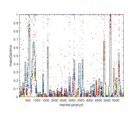
(a) Posterior means of $\gamma_{jt}$

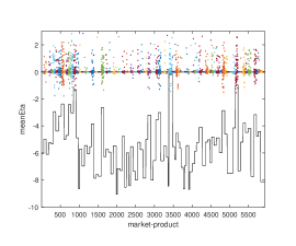
(b) Posterior means of $\eta_{jt}$

(a): for each market $t$, the colored dots refer to posterior means of $\gamma_{jt}$’s and the solid line is the posterior mean of $\phi_{t}$. The prior mean of $\phi_{t}$ is 0.5. (b): the colored dots represent posterior means of $\eta_{jt}$’s and the solid line is the posterior mean of $\bar{\xi}_{t}$. $\xi_{jt}$ is the vertical sum. 5927 market-product pairs. 95 markets (stores).

The colored dots in Figure 1(a) show the posterior means of $\gamma_{jt}$’s. A smaller $\gamma_{jt}$ means that market-product pair $(jt)$ is more likely in the sparse set $\mathcal{K}_{t}$. Different colors of these dots correspond to different markets. Among the 5927 market-product pairs in the sample, there are only 658 pairs with posterior mean of $\gamma_{jt}$ greater than 0.5, meaning that the majority of $\xi_{jt}$’s are shrunk towards the market-specific values $\bar{\xi}_{t}$ with high probability.

Figure 1(b) illustrates the posterior means of the shocks $\eta_{jt}$ as colored dots and the market-specific intercepts $\bar{\xi}_{t}$ as solid lines. By definition, the posterior mean of $\xi_{jt}$ is obtained by vertically summing $\eta_{jt}$ and $\bar{\xi}_{t}$. As expected, most $\eta_{jt}$’s are effectively zero, confirming a high degree of sparsity in the data. An interesting pattern emerges: the distribution of $\eta_{jt}$ is right-skewed, with more $(jt)$ pairs exhibiting positive $\eta_{jt}$’s than negative ones. These positive $\eta_{jt}$’s likely capture store-product level promotion efforts, as discussed earlier.

The estimated market-product demand shocks reflect promotional efforts. To evaluate how much of these efforts are explained by the observed marketing mix variables, namely display and feature indicators, we regress the estimated $\eta_{jt}$’s on these variables. Table 5 presents the regression results for both the shrinkage and BLP approaches. The slopes on the marketing mix variables are positive and significant in both cases, suggesting that $\eta_{jt}$ effectively captures store-product-level promotion activities. However, based on the $R^{2}$, the marketing mix indicator variables explain only 2.5% of the estimated promotion efforts, highlighting the presence of potentially substantial unobserved store-level marketing activities. This finding underscores the noisiness of the marketing mix variables in capturing store promotions and emphasizes the importance of incorporating the market-product demand shocks $\xi_{jt}$’s into the model.

Table 5: Regression of the estimated $\eta_{jt}$’s on marketing mix variables.

	Shrinkage		BLP
Intercept	0.046	( 0.036, 0.0554 )	-0.059	( -0.089, -0.030 )
Display	0.287	( 0.220, 0.355 )	0.722	( 0.507, 0.937 )
Feature	0.101	( 0.072, 0.130 )	0.393	( 0.300, 0.487 )
Adjusted R2	0.0248		0.0236

• Estimated slopes with 95% confidence intervals in parentheses.

Finally, we examine product-level price elasticities, which are a key output of demand estimation. As mentioned earlier, once MCMC draws are obtained, computing point and interval estimates of elasticity is straightforward, representing a key advantage of the proposed approach. Table 6 presents posterior means and 95% credible intervals of own-price elasticity for selected products in a market, sorted by price. For comparison, the table also includes elasticity estimates based on the BLP approach and the simple logit model (IV and OLS).

One notable observation is that when random coefficients (particularly on price) are incorporated, as in the shrinkage and BLP approaches, a U-shaped relationship between price and elasticity emerges, consistent with findings in the literature, such as Berry . (1995). In contrast, the simple logit model shows a monotonic increase in elasticity with price. Furthermore, the magnitudes of the elasticities estimated by our procedure are reasonable, and all products exhibit elastic demand (i.e., greater than 1).

Table 6: Price elasticity of some products in a market

	Own Price Elasticities
Product	Price	Bayesian Shrinkage		BLP	Logit-IV	Logit-OLS
PRIVATE LABEL Nonfat Size 4	1.495	-1.41	( -1.54 , -1.30 )	-1.19	-0.64	-0.84
AXELROD Lowfat Size 4	1.645	-1.50	( -1.65 , -1.39 )	-1.27	-0.70	-0.92
DANNON ACTIVIA Flavored Lowfat Size 3	2.660	-1.97	( -2.21 , -1.83 )	-1.66	-1.13	-1.49
BROWN COW Flavored Greek Size 1	3.973	-2.11	( -2.49 , -1.82 )	-1.66	-1.70	-2.23
CHOBANI Flavored Lowfat Greek Size 1	4.452	-2.06	( -2.48 , -1.68 )	-1.52	-1.90	-2.50
CHOBANI Flavored Nonfat Greek Size 1	4.470	-2.05	( -2.48 , -1.67 )	-1.52	-1.91	-2.51
FAGE TOTAL Nonfat Greek Size 2	4.536	-2.05	( -2.48 , -1.65 )	-1.49	-1.94	-2.54
DANNON GREEK Nonfat Greek Size 1	5.403	-1.85	( -2.38 , -1.32 )	-1.08	-2.31	-3.03
THE GREEK GODS Nonfat Greek Size 1	5.840	-1.72	( -2.30 , -1.13 )	-0.82	-2.50	-3.27
FAGE TOTAL Nonfat Greek Size 1	6.579	-1.48	( -2.14 , -0.80 )	-0.38	-2.81	-3.69

• The 95% credible intervals for the shrinkage approach shown in parentheses.

5.2 Revisit the BLP Auto Data

We revisit the classic BLP application to the U.S. automobile market. The BLP auto dataset contains product-level prices, quantities, and characteristics for major car models in the U.S. market for each year from 1971 to 1990. Following Berry . (1995), we define each year as a market, resulting in 20 markets ($T=20$) and an average of approximately 110 products per market. A detailed description of the dataset is provided in Berry, Levinsohn  Pakes (1995).

This additional application is valuable for several reasons. First, the industry context differs sharply: the automobile market involves durable goods and large, infrequent purchases, whereas the yogurt market represents low-cost grocery items and frequent consumption. Second, the scope of the data is distinct: the auto dataset captures national-level demand for automobiles, while the yogurt application focuses on highly disaggregated store-level activities. By applying our method to these two contrasting settings, we demonstrate its flexibility in uncovering sparse demand shocks in distinct scenarios with diverse market structures and datasets.

We consider a similar model structure as in the yogurt application. The product characteristics ($X_{jt}$) include price, horsepower/weight (log), weight (log), size (log), dollar/mile (log), and indicators for air conditioning, power steering, automatic transmission, and forward drive ($d_{X}=9$). Random coefficients on $X_{jt}$ follow $\beta_{i}\sim N_{d_{X}}(\bar{\beta},\Sigma)$, where $\Sigma=\text{diag}(\sigma_{1}^{2},\ldots,\sigma_{d_{X}}^{2})$. The market-product shocks ($\xi_{jt}$) are decomposed into market fixed effects ($\bar{\xi}_{t}$) and product-specific deviations ($\eta_{jt}$).

This specification differs from Berry . (1995) in two key ways: (1) it excludes a supply-side model, and (2) it includes market fixed effects to account for market-level heterogeneity. Our goal is not to replicate their results but to demonstrate how our approach can uncover sparsity in this classic dataset.

Compared to the yogurt application, the auto dataset differs in several aspects. While the yogurt data feature more markets and fewer products per market, the auto dataset includes fewer markets (20 years) but an average of 110 products per market, totaling 2,217 market-product pairs. As in the yogurt case, the number of parameters exceeds the number of independent first-order conditions, making sparsity assumptions on $\eta_{jt}$ essential to restore identification. We use our shrinkage approach for estimation, following the same MCMC procedure. Again, for comparison, we include the standard BLP GMM estimator, with IVs constructed by interacting the BLP IVs with market dummies, as well as simple logit specifications (OLS and IV).

Table 7: Estimation results for the automobile application: preference parameters

	Random Coefficient Logit				Simple Logit
	Bayesian Shrinkage		BLP		IV	OLS
	Mean of RC	S.D. of RC	Mean of RC	S.D. of RC
Price	-0.29	0.12	-0.42	0.15	-0.10	-0.08
	(-0.41, -0.2)	(0.09, 0.17)	(-0.48, -0.36)	(0.13, 0.17)	(-0.11, -0.09)	(-0.09, -0.07)
HP/Weight (log)	-0.46	1.02	0.02	1.22	0.65	0.50
	(-1.4, 0.19)	(0.64, 1.65)	(-0.46, 0.51)	(0.77, 1.68)	(0.44, 0.85)	(0.24, 0.77)
Weight (log)	-0.56	0.57	0.38	0.09	-0.67	-1.45
	(-1.64, 0.42)	(0.23, 1.04)	(-0.41, 1.17)	(0, 1.29)	(-1.27, -0.08)	(-2.17, -0.74)
Size (log)	3.65	0.88	3.67	0.17	5.09	5.65
	(2.41, 4.73)	(0.3, 1.61)	(2.80, 4.44)	(0, 2.63)	(4.44, 5.73)	(4.83, 6.48)
Dollar/Mile (log)	-2.99	1.6	-1.36	0.69	-1.39	-1.14
	(-4.01, -2.12)	(0.99, 2.27)	(-1.86, -0.85)	(0.12, 1.25)	(-1.67, -1.12)	(-1.53, -0.75)
AC	0.39	0.39	0.66	0.38	0.25	.05
	(0.07, 0.71)	(0.2, 0.82)	(0.45, 0.87)	(0.02, 0.74)	(0.13, 0.37)	(-0.10, 0.20)
Power Steering	0.05	0.6	0.08	0.08	-0.19	-.28
	(-0.21, 0.3)	(0.34, 0.95)	(-0.07, 0.24)	(0, 0.53)	(-0.29, -0.09)	(-0.43, -0.14)
Automatic	0.12	0.42	0.30	0.03	0.28	.27
	(-0.1, 0.36)	(0.19, 0.76)	(0.14, 0.45)	(0, 0.50)	(0.18, 0.39)	(0.14, 0.41)
FWD	0.08	0.36	0.03	0.72	0.10	.15
	(-0.15, 0.29)	(0.17, 0.79)	(-0.11 0.16)	(0.48, 0.96)	(0.01, 0.18)	(0.03, 0.27)
Market FE	Omitted
	Own Price Elasticity
Mean	-1.52		-2.38		-1.06	-1.18
S.D.	0.49		0.96		0.78	0.86

• Note: The table reports estimated preference parameters with the 95% credible/confidence intervals, as well as means and standard deviations of own-price elasticities.

• When the left end of the confidence interval for a SD of RC is negative, we replace it with 0 to respect the non-negative constraint on the parameter.

The estimation results for the preference parameters ($\beta$ and $\Sigma$) are presented in Table 7. For the mean random coefficients, our Bayesian shrinkage approach yields estimates with reasonable signs and magnitudes, closely aligning with those of the standard BLP estimates. Regarding the standard deviations (SDs) of random coefficients, the Bayesian shrinkage approach indicates considerable dispersion for all random coefficients, suggesting rich heterogeneity in consumers’ tastes across all product characteristics. In contrast, several SDs from the BLP estimates, including those for weight, size, power steering, and automatic transmission, are virtually zero. These near-zero estimates may be attributed to the weak IV problem, as highlighted by Reynaert  Verboven (2014). Furthermore, while the BLP estimator is sensitive to the choice of IVs - based on our experiments with the data, though specific results are not reported here - our Bayesian shrinkage approach is immune to this issue, making it a particularly advantageous tool in practice.

Figure 2: Estimated sparsity structure in the automobile data.

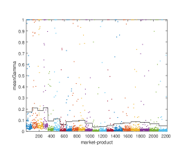
(a) Posterior means of $\gamma_{jt}$

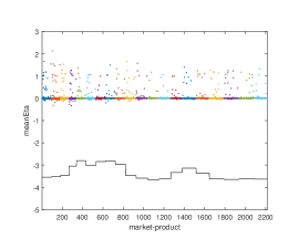
(b) Posterior means of $\eta_{jt}$

(a): for each market $t$, the colored dots refer to posterior means of $\gamma_{jt}$’s and the solid line is the posterior mean of $\phi_{t}$. The prior mean of $\phi_{t}$ is 0.5. (b): the colored dots represent posterior means of $\eta_{jt}$’s and the solid line is the posterior mean of $\bar{\xi}_{t}$. $\xi_{jt}$ is the vertical sum. 2217 market-product pairs. 20 markets (years 1971-1990).

Now, we turn to the latent sparsity structure of the market-product shocks $\eta_{jt}$ identified by our procedure, as summarized in Figure 2. This figure serves as the counterpart to Figure 1 from the yogurt application. Overall, we find stronger evidence of sparsity in this dataset compared to the yogurt data. The solid lines in Figure 2(a) show the posterior means of $\phi_{t}$’s, which indicate sparse markets. The average posterior mean is notably small, at 0.098, with particularly low values (less than 0.05) observed in the 1982, 1983, and 1990 markets. Among the 2,217 market-product pairs in this dataset, only 133 have a posterior mean of $\gamma_{jt}$ greater than 0.5, represented by the colored dots. Additionally, Figure 2(b) reveals that the distribution of $\eta_{jt}$ is right-skewed, a pattern consistent with the yogurt application.

6 Conclusion

In this paper, we have proposed a new approach to estimating the random coefficient logit demand model with sparse market-product level demand shocks. Our approach eliminates the need for instrumental variables (IVs), which are required in the standard BLP GMM method. We show that, under certain regularity conditions, the demand shocks and their sparsity structure can be identified along with other model parameters. We also propose a Bayesian shrinkage estimation procedure that offers a scalable and flexible alternative to existing methods.

We demonstrate the applicability of our approach through two empirical applications. First, in the context of supermarket scanner data, we interpret the demand shocks as unobserved promotion efforts at the store-week level, capturing the sparsity in promotional activities across products. Second, we revisit the automotive market, where we model unobserved advertising efforts as demand shocks and show how our method identifies the underlying structure of these shocks across brands and models. In both cases, we find strong evidence of sparsity in demand shocks, supporting the relevance of the sparsity assumption in real-world data.

Appendix A Mathematical Proofs

A.1 Proof of Lemma 1

Proof.

For any $t$, consider the demand functions for the first $K_{t}+1$ products

$$\sigma_{jt}\left(\xi_{t},f\right)=\int\frac{\exp\left(X_{jt}^{\top}\beta+\xi_{jt}\right)}{1+\sum_{k=1}^{K_{t}}\exp\left(X_{kt}^{\top}\beta+\xi_{kt}\right)+\sum_{k=K_{t}+1}^{J_{t}}\exp\left(X_{kt}^{\top}\beta+\nu_{t}\right)}f\left(\beta\right)d\beta,\>j=1,...,K_{t}+1.$$ (16)

Fixing any $f\in\mathcal{F}$, we will show that the $(K_{t}+1)$-dimensional system

$$s_{jt}=\sigma_{jt}\left(\xi_{t},f\right),j=1,...,K_{t}+1$$ (17)

uniquely determines $\left(\xi_{1t},...,\xi_{K_{t}t},\nu_{t}\right)$.

Following the argument in the Appendix of Berry (1994), we just need to show the Jacobian matrix of the system (17) has a dominant diagonal, i.e.,

$$\frac{\partial\sigma_{jt}\left(\xi_{t},f\right)}{\partial\xi_{jt}}>\sum_{m\neq j}\left|\frac{\partial\sigma_{jt}\left(\xi_{t},f\right)}{\partial\xi_{mt}}\right|,\>\forall j=1,...,K_{t}+1,$$ (18)

where $\xi_{K_{t}+1,t}=\nu_{t}$.

Observe that

$$\sum_{m=1}^{K_{t}+1}\frac{\partial\sigma_{jt}\left(\xi_{t},f\right)}{\partial\xi_{mt}}=\int\dot{\sigma}_{jt}\left(\beta,\xi_{t},f\right)\left[1-\sum_{m=1}^{K_{t}+1}\dot{\sigma}_{mt}\left(\beta,\xi_{t},f\right)\right]f\left(\beta\right)d\beta>0,$$

where

$$\dot{\sigma}_{jt}\left(\beta,\xi_{t},f\right)\equiv\frac{\exp\left(X_{jt}^{\top}\beta+\xi_{jt}\right)}{1+\sum_{k=1}^{K_{t}}\exp\left(X_{kt}^{\top}\beta+\xi_{kt}\right)+\sum_{k=K_{t}+1}^{J_{t}}\exp\left(X_{kt}^{\top}\beta+\nu_{t}\right)}.$$

Also, it is straightforward to verify that $\frac{\partial\sigma_{jt}\left(\xi_{t},f\right)}{\partial\xi_{jt}}>0$ for all $j$ and $\frac{\partial\sigma_{jt}\left(\xi_{t},f\right)}{\partial\xi_{kt}}<0$ for any $k\neq j$. These inequalities imply that the dominant diagonal condition (18) holds. ∎

A.2 Proof of Theorem 1

Proof.

Note that for any market $t$ and product $j\geq K_{t}+1$, the demand function can be written as

$$\sigma_{jt}\left(\xi_{t},f\right)= \int\frac{\exp\left(X_{jt}^{\top}\beta+\nu_{t}\right)}{1+\sum_{k=1}^{K_{t}}\exp\left(X_{kt}^{\top}\beta+\xi_{kt}\right)+\sum_{k=K_{t}+1}^{J_{t}}\exp\left(X_{kt}^{\top}\beta+\nu_{t}\right)}f\left(\beta\right)d\beta$$

$$= \int\frac{\exp\left(X_{jt}^{\top}\beta\right)}{\left[1+\sum_{k=1}^{K_{t}}\exp\left(X_{kt}^{\top}\beta+\xi_{kt}\right)\right]\exp\left(-\nu_{t}\right)+\sum_{k=K_{t}+1}^{J_{t}}\exp\left(X_{kt}^{\top}\beta\right)}f\left(\beta\right)d\beta.$$

Substitute $\xi_{jt}$ with the inverse demand function $\tilde{\sigma}_{jt}^{-1}\left(\tilde{s}_{t},f\right)$, we can obtain

$$\sigma_{jt}\left(\tilde{\sigma}_{t}^{-1}\left(\tilde{s}_{t},f\right),f\right)=\int\frac{\exp\left(X_{jt}^{\top}\beta\right)}{\exp\left[H_{t}\left(\beta,f\right)\right]}f\left(\beta\right)d\beta,$$ (19)

where

$$H_{t}\left(\beta,f\right)\equiv\log\left\{\left[1+\sum_{k=1}^{K_{t}}\exp\left(X_{kt}^{\top}\beta+\tilde{\sigma}_{kt}^{-1}\left(\tilde{s}_{t},f\right)\right)\right]\exp\left(-\tilde{\sigma}_{K_{t}+1,t}^{-1}\left(\tilde{s}_{t},f\right)\right)+\sum_{k=K_{t}+1}^{J_{t}}\exp\left(X_{kt}^{\top}\beta\right)\right\}.$$

Given market $t$, note that the right-hand-side of (19) varies by $j$ only through $X_{jt}$, so we can define a market share function $\bar{\sigma}_{t}\left(\cdot\right)$ that does not have subscript $j$, i.e.,

$$\bar{\sigma}_{t}\left(X_{jt},f\right)\equiv\sigma_{jt}\left(\tilde{\sigma}_{t}^{-1}\left(\tilde{s}_{t},f\right),f\right).$$

Now consider the Laplace transform of the function $\frac{f\left(\beta\right)}{\exp\left[H_{t}\left(\beta,f\right)\right]}$,

$$\bar{\sigma}_{t}\left(x,f\right)=\int\frac{\exp\left(x^{\top}\beta\right)f\left(\beta\right)}{\exp\left[H_{t}\left(\beta,f\right)\right]}d\beta,\>\forall x\in\mathcal{B},$$ (20)

where $\mathcal{B}$ is some bounded open $\mathbf{R}^{d_{X}}$-ball and Assumption 3 ensures the transform is well-defined. By the uniqueness of the inverse Laplace transform (see, e.g., the Theorem 6b of Widder (1941)), if $\bar{\sigma}_{t}\left(x,f\right)=\bar{\sigma}_{t}\left(x,f^{0}\right)$ for all $x\in\mathcal{B}$, then

$$\frac{f\left(\beta\right)}{\exp\left[H_{t}\left(\beta,f\right)\right]}=\frac{f^{0}\left(\beta\right)}{\exp\left[H_{t}\left(\beta,f^{0}\right)\right]}$$ (21)

for all $\beta$.

Next, we will show that the only $f$ that satisfies (21) for all markets is $f=f^{0}$, where $f^{0}$ denotes the true value of $f$. For any $f\neq f^{0}$, there exists some $b_{1}\neq 0$ and $b_{2}\neq 0$ such that $f\left(b_{1}\right)>f^{0}\left(b_{1}\right)$ and $f\left(b_{2}\right)<f^{0}\left(b_{2}\right)$. Observe that for any $\beta$

$$\begin{split}&\exp\left[H_{t}\left(\beta,f\right)\right]-\exp\left[H_{t}\left(\beta,f^{0}\right)\right]\\ =&\left[1+\sum_{k=1}^{K_{t}}\exp\left(X_{kt}^{\top}\beta+\tilde{\sigma}_{kt}^{-1}\left(\tilde{s}_{t},f\right)\right)\right]\exp\left(-\tilde{\sigma}_{K_{t}+1,t}^{-1}\left(\tilde{s}_{t},f\right)\right)\\ -&\left[1+\sum_{k=1}^{K_{t}}\exp\left(X_{kt}^{\top}\beta+\tilde{\sigma}_{kt}^{-1}\left(\tilde{s}_{t},f^{0}\right)\right)\right]\exp\left(-\tilde{\sigma}_{K_{t}+1,t}^{-1}\left(\tilde{s}_{t},f^{0}\right)\right)\\ =&\Delta_{K_{t}+1,t}\left(f,f^{0}\right)+\sum_{k=1}^{K_{t}}\exp\left(X_{kt}^{\top}\beta\right)\tilde{\Delta}_{k,t}\left(f,f^{0}\right),\end{split}$$ (22)

where

$$\Delta_{K_{t}+1,t}\left(f,f^{0}\right)=\exp\left(-\tilde{\sigma}_{K_{t}+1,t}^{-1}\left(\tilde{s}_{t},f\right)\right)-\exp\left(-\tilde{\sigma}_{K_{t}+1,t}^{-1}\left(\tilde{s}_{t},f^{0}\right)\right),$$

$$\tilde{\Delta}_{k,t}\left(f,f^{0}\right)=\exp\left[\tilde{\sigma}_{kt}^{-1}\left(\tilde{s}_{t},f\right)-\tilde{\sigma}_{K_{t}+1,t}^{-1}\left(\tilde{s}_{t},f\right)\right]-\exp\left[\tilde{\sigma}_{kt}^{-1}\left(\tilde{s}_{t},f^{0}\right)-\tilde{\sigma}_{K_{t}+1,t}^{-1}\left(\tilde{s}_{t},f^{0}\right)\right].$$

Note that the terms $\Delta_{K_{t}+1,t}\left(f,f^{0}\right)$ and $\tilde{\Delta}_{k,t}\left(f,f^{0}\right)$ (for any $k$) do not depend on $\beta$. For any given $f$, let us examine the sign of (22) in the following three cases. First, if

$$\min\left\{\Delta_{K_{t}+1,t}\left(f,f^{0}\right),\min_{k\in\left\{1,...,K_{t}\right\}}\left[\tilde{\Delta}_{k,t}\left(f,f^{0}\right)\right]\right\}>0,$$

then (22) is positive for any $\beta$ and thus (21) does not hold at $b_{2}$. Second, if

$$\max\left\{\Delta_{K_{t}+1,t}\left(f,f^{0}\right)<0,\max_{k\in\left\{1,...,K_{t}\right\}}\left[\tilde{\Delta}_{k,t}\left(f,f^{0}\right)\right]\right\}<0,$$

then (22) is negative for any $\beta$ and thus (21) does not hold at $b_{1}$. Third, if

$$\min\left\{\Delta_{K_{t}+1,t}\left(f,f^{0}\right),\min_{k\in\left\{1,...,K_{t}\right\}}\left[\tilde{\Delta}_{k,t}\left(f,f^{0}\right)\right]\right\}<0$$

and

$$\max\left\{\Delta_{K_{t}+1,t}\left(f,f^{0}\right)<0,\max_{k\in\left\{1,...,K_{t}\right\}}\left[\tilde{\Delta}_{k,t}\left(f,f^{0}\right)\right]\right\}>0,$$

then (22) can be positive or negative depending on the vector $\left(X_{1t}^{\top}\beta,...,X_{K_{t},t}^{\top}\beta\right)$. Assumption 2 implies that for any finite $\beta$, the random vector $\left(X_{1t}^{\top}\beta,...,X_{K_{t},t}^{\top}\beta\right)$ has full support in $\mathbf{R}^{K_{t}}$. Thus (22) can be positive (or negative) with positive probability for any $\beta$; it follows that (21) does not hold at $b_{2}$ (or $b_{1}$) with positive probability.

Hence, for any $f\neq f^{0}$, there exists some $x\in\mathcal{B}$ such that $\bar{\sigma}_{t}\left(x,f\right)\neq\bar{\sigma}_{t}\left(x,f^{0}\right)$ with a positive probability. Due to the continuity of both sides of the inequality in $x$, the inequality holds for all $x$ in a subset of $\mathcal{B}$ with a positive probability. Thus $f^{0}$ is identified. Furthermore, given $f^{0}$, Lemma 1 implies that $\left\{\xi_{jt}^{0}\right\}_{j,t}$ ($\xi_{jt}^{0}$ denotes the true value) are identified, which concludes the proof.

∎

Appendix B Computation Details of the MCMC Procedure

In this section, we describe how the model is estimated in the proposed approach. Recall that we have the $d_{X}$-dimensional slope parameter $\bar{\beta}$, the log standard deviations for the random coefficients $r=(r_{1},\ldots,r_{d_{X}})^{\prime}$, the market-specific intercepts $\bar{\xi}=\{\bar{\xi}_{1},\ldots,\bar{\xi}_{T}\}$, the market-product specific deviations $\eta=\{\eta_{1},\ldots,\eta_{T}\}$, where $\eta_{t}=(\eta_{1t},\ldots,\eta_{J_{t}t})^{\prime}$, the binary indicator variables $\Gamma=\{\gamma_{1},\ldots,\gamma_{T}\}$, where $\gamma_{t}=(\gamma_{1t},\ldots,\gamma_{J_{t}t})^{\prime}$, and the inclusion probabilities $\phi=(\phi_{1},\ldots,\phi_{T})^{\prime}$. The data contains the quantity demanded $q=\{q_{1},\ldots,q_{T}\}$, where $q_{t}=\{q_{1t},\ldots,q_{J_{t}t}\}$ and the market-level covariates $X=\{X_{1},\ldots,X_{T}\}$. We obtain a posterior sample $\{\bar{\beta}^{(g)},r^{(g)},\bar{\xi}^{(g)},\eta^{(g)},\Gamma^{(g)},\phi^{(g)}\}_{g=1}^{G}$, where $G$ is the total number of MCMC draws (after discarding an appropriate burn-in draws). The MCMC itertaes the following steps. The order of the updates is arbitrary.

$$\text{Draw }\bar{\beta}^{(g+1)}\text{ given } \bar{\beta}^{(g)},\underline{\mu}_{\beta},\ \underline{V}_{\beta},\ r^{(g)},\ \bar{\xi}^{(g)},\ \eta^{(g)},\ q,\ X$$

$$\text{Draw }r^{(g+1)}\text{ given } r^{(g)},\{\underline{V}_{r,k}\},\ \bar{\beta}^{(g+1)},\ \bar{\xi}^{(g)},\ \eta^{(g)},\ q,\ X$$

$$\text{Draw }\bar{\xi}^{(g+1)}\text{ given } \bar{\xi}^{(g)},\{\underline{\mu}_{\xi_{t}},\underline{V}_{\xi_{t}}\},\ \bar{\beta}^{(g+1)},\ r^{(g+1)},\ \eta^{(g)},\ q,\ X$$

$$\text{Draw }\eta^{(g+1)}\text{ given } \eta^{(g)},\Gamma,\ \tau^{2}_{0},\ \tau^{2}_{1},\ \bar{\beta}^{(g+1)},\ r^{(g+1)},\ \bar{\xi}^{(g+1)},\ q,\ X$$

$$\text{Draw }\Gamma^{(g+1)}\text{ given } \eta^{(g+1)},\ \tau^{2}_{0},\ \tau^{2}_{1},$$

$$\text{Draw }\phi^{(g+1)}\text{ given } \Gamma^{(g+1)},\ \underline{a}_{\phi},\ \underline{b}_{\phi}.$$

Below, we illustrate how to conduct the updates above i.e. how to sample from the conditional posterior distributions of the parameters. Each of the conditional distributions below are defined given all other parameters, the hyperparameters, and the data, which are denoted by $\bullet$.

B.1 Sampling $\bar{\beta},\bar{\xi},\eta,r$

The conditional posterior for $(\bar{\beta},\bar{\xi},\eta,r)$ is

$$\pi(\bar{\beta},\bar{\xi},\eta,r|\bullet)\propto p\left(\bar{\beta},r,\bar{\xi}_{1},...,\bar{\xi}_{T},\eta_{1},\ldots,\eta_{T},r|q\right)\cdot\pi(\bar{\beta})\cdot\pi(\bar{\xi})\cdot\pi(\eta)\cdot\pi(r),$$

where

$$p\left(\bar{\beta},r,\bar{\xi}_{1},...,\bar{\xi}_{T},\eta_{1},\ldots,\eta_{T},r|q\right)=\prod_{t=1}^{T}\prod_{j=0}^{J_{t}}\left[\sigma_{jt}\left(\xi_{t},\bar{\beta},r\right)\right]^{q_{jt}}$$

is the likelihood function and $\pi(\cdot)$ is the prior. The conditional posterior does not belong to a known class of distributions, so we employ a Metropolis–Hastings (M-H) algorithm to sample these parameters. One could update $\bar{\beta},\bar{\xi},\eta$, and $r$ in one block, but the dimensionality of the parameter vector to be sampled is typically large (e.g. $d_{X}+T+TJ+d_{X}$ $>2,000$ in the auto market application), and the sampling might be inefficient. To increase the computational speed and avoid calculation of cross-derivatives, the parameter subvectors $\bar{\beta},\bar{\xi},\eta$, and $r$ are set to be independent in the proposal. Furthermore, note that conditional on $\bar{\beta}$ and $r$, updating of $\{\bar{\xi}_{t}\}$ and $\{\eta_{jt}\}$ can be done independently over market $t$.

Specifically, for each $\theta\in\{\bar{\beta},\eta\}$, we use a tailored Metropolis–Hastings (TMH) algorithm to sample $\theta$ from its conditional posterior (Chib  Greenberg, 1995). First, the mode of the conditional posterior, $\hat{\theta}$ is obtained

$$\hat{\theta}=\arg\max_{\theta}\log\left[L(\theta|\bullet)\pi(\theta)\right],$$

where $L(\theta|\bullet)$ is the likelihood function relevant to $\theta$ and $\pi(\theta)$ is the prior. The maximization is performed by a Newton’s method. At iteration $g$, let $\theta^{(g)}$ be the value of $\theta$. A candidate value is drawn as

$$\tilde{\theta}\sim N_{\text{dim}(\theta)}\left(\hat{\theta}^{(g)},\kappa^{2}_{\theta}\hat{V}_{\theta}\right),$$

where

$$\hat{V}_{\theta}^{-1}=-\frac{\partial^{2}}{\partial\theta\partial\theta^{\prime}}\log L(\theta|\bullet)\pi(\theta)\bigg{|}_{\theta=\hat{\theta}}.$$

This candidate is accepted with probability

$$\min\left\{\frac{\pi(\tilde{\theta}|\bullet)\phi(\theta^{(g)}|\hat{\theta},\hat{V}_{\theta})}{\pi(\theta^{(g)}|\bullet)\phi(\tilde{\theta}|\hat{\theta},\hat{V}_{\theta})},1\right\},$$

where $\phi(\ \ )$ denotes the density of normal distribution. We fix $\kappa_{\theta}$ at $2.38\ \text{dim}(\theta)^{-0.5}$, and if necessary, we tune it based on draws from a short chain that was run for the purpose of calibrating in order to achieve acceptance rate between 0.3 and 0.5. The likelihood is known to be concave with respect to each $\theta\in\{\bar{\beta},\eta\}$ under the Gumbel error distribution, so the convergence to $\hat{\theta}$ is fast and only requires a few iterations in many cases. The gradients and Hessians of the log-likelihood with respect to $\bar{\xi}$ and $r$ are also available and so TMH can be used, but the random-walk MH works efficiently for updating these parameters based on our experience, which we describe below.

B.1.1 Sampling $\bar{\beta}$

The conditional posterior for $\bar{\beta}$ is

$$\pi(\bar{\beta}|\bullet)\propto p\left(\bar{\beta},r,\bar{\xi}_{1},...,\bar{\xi}_{T},\eta_{1},\ldots,\eta_{T}|q\right)\cdot\pi(\bar{\beta}),$$

where

$$p\left(\bar{\beta},r,\bar{\xi}_{1},...,\bar{\xi}_{T},\eta_{1},\ldots,\eta_{T}|q\right)=\prod_{t=1}^{T}\prod_{j=0}^{J_{t}}\left[\sigma_{jt}\left(\xi_{t},\bar{\beta},r\right)\right]^{q_{jt}}$$

is the likelihood function and $\pi(\cdot)$ is the prior.

B.1.2 Sampling $\eta_{jt}$

The conditional posterior for $\eta_{t}=(\eta_{1t},\ldots,\eta_{J_{t}t})^{\prime}$ is independent over $t$ and

$$\pi(\eta_{t}|\bullet)\propto p\left(\bar{\beta},r,\bar{\xi}_{t},\eta_{t}|q_{t}\right)\cdot\prod_{j=1}^{J_{t}}\phi(\eta_{jt}|0,\gamma_{jt}\tau^{2}_{1}+(1-\gamma_{jt})\tau^{2}_{0}),$$

for $t=1,\ldots,T$, where

$$p\left(\bar{\beta},r,\bar{\xi}_{t},\eta_{t}|q_{t}\right)=\prod_{j=0}^{J_{t}}\left[\sigma_{jt}\left(\xi_{t},\bar{\beta},r\right)\right]^{q_{jt}},$$

is the market $t$’s likelihood contribution.

B.1.3 Sampling $\bar{\xi}_{t}$

The conditional posterior for $\bar{\xi}_{t}$ is independent over $t$ and

$$\pi(\bar{\xi}_{t}|\bullet)\propto p\left(\bar{\beta},r,\bar{\xi}_{t},\eta_{t}|q_{t}\right)\cdot\pi(\bar{\xi}_{t}),$$

for $t=1,\ldots,T$. We employ a random walk Metropolis-Hastings (RWMH) algorithm to sample from the conditional posterior. At iteration $g$, let $\bar{\xi}_{t}^{(g)}$ be the value of $\bar{\xi}_{t}$. A candidate value is drawn as

$$\tilde{\bar{\xi}}_{t}\sim N\left(\bar{\xi}_{t}^{(g)},\kappa_{\xi}^{2}\underline{S}_{\xi}\right),$$

where $\underline{S}_{\xi}$ is a fixed scalar and $\kappa_{\xi}$ is a scaling constant. We let $\underline{S}_{\xi}=1$. We run an initial MCMC for the purpose of calibrating $\kappa_{\xi}$ to achieve acceptance rate between 0.3 and 0.5. This candidate is accepted with probability

$$\min\left\{\frac{\pi(\tilde{\bar{\xi}}_{t}|\bullet)}{\pi(\bar{\xi}_{t}^{(g)}|\bullet)},1\right\}.$$

B.1.4 Sampling $r$

The conditional posterior distribution of $r$ is

$$\pi(r|\bullet)\propto p\left(\bar{\beta},r,\bar{\xi}_{1},...,\bar{\xi}_{T},\eta_{1},\ldots,\eta_{T}|q\right)\cdot\pi(r),$$

where $p\left(\bar{\beta},r,\bar{\xi}_{1},...,\bar{\xi}_{T},\eta_{1},\ldots,\eta_{T}|q\right)$ is the likelihood function and $\pi(\cdot)$ is the prior. We employ a random walk Metropolis-Hastings (RWMH) algorithm to sample from the conditional posterior. At iteration $g$, let $r^{(g)}$ be the value of $r$. A candidate value is drawn as

$$\tilde{r}\sim N_{K}\left(r^{(g)},\kappa_{r}\underline{S}_{r}\right),$$

where $\underline{S}_{r}$ is a $K\times K$ scale matrix and $\kappa_{r}$ is a scaling constant. We run an initial MCMC for the purpose of calibration. We first tune $\kappa_{r}$ to achieve acceptance rate between 0.3 and 0.5, and set $\underline{S}_{r}$ as the estimated covariance matrix of the draws. This candidate is accepted with probability

$$\min\left\{\frac{\pi(\tilde{r}|\bullet)}{\pi(r^{(g)}|\bullet)},1\right\}.$$

B.2 Sampling $\gamma_{jt}$

We can derive the conditional posterior distribution of the binary indicator $\gamma_{jt}$, which is the Bernoulli distribution with the following success probability:

$$\Pr(\gamma_{jt}=1|\bullet)=\frac{\phi_{t}\cdot\phi(\eta_{jt}|0,\tau^{2}_{1})}{(1-\phi_{t})\cdot\phi(\eta_{jt}|0,\tau^{2}_{0})+\phi_{t}\cdot\phi(\eta_{jt}|0,\tau^{2}_{1})},$$ (23)

independently for $j=1,\ldots,J_{t}$ and $t=1,\ldots,T$.

B.3 Sampling $\phi$

Under the conjugate prior i.e. $\phi_{t}\sim\text{Beta}(\underline{a}_{\phi},\underline{b}_{\phi})$, the posterior conditional distribution is available in the closed form:

$$\phi_{t}|\bullet\sim\text{Beta}\left(\underline{a}_{\phi}+\sum_{j=1}^{J_{t}}\gamma_{jt},\underline{b}_{\phi}+\sum_{j=1}^{J_{t}}(1-\gamma_{jt})\right),$$ (24)

independently for $t=1,\ldots,T$.

Appendix C Computing Price Elasticities

Price elasticities are a key output of demand estimation and provide a description of the substitution patterns among competing products implied by the estimated model. Importantly, elasticities are functions of the model parameters, and therefore, the posterior draws can be conveniently used for their uncertainty quantification. For example, after implementing the proposed MCMC, one can easily construct credible intervals for elasticities based on the following formulas.

The demand elasticity of product $j$ with respect to the price change in product $m$ in market $t$ is

$$E_{jm,t}(\xi_{t},\bar{\beta},r)=\frac{\%\Delta\sigma_{jt}}{\%\Delta p_{mt}}=\frac{p_{mt}}{\sigma_{jt}(\xi_{t},\bar{\beta},r)}\cdot\frac{\partial\sigma_{jt}(\xi_{t},\bar{\beta},r)}{\partial p_{mt}},$$ (25)

where $p_{jt}$ is the observed price of product $j$ in market $t$, $\beta_{price}$ is the slope on price, and $\sigma_{jt}$ is the model-predicted market share. The last term can be written as

$$\frac{\partial\sigma_{jt}(\xi_{t},\bar{\beta},r)}{\partial p_{mt}}=\int\beta_{price,i}\cdot\frac{\partial\sigma_{ijt}}{\partial\delta_{mt}}f(\beta_{i})d\beta_{i}=\int\left(\bar{\beta}_{price}+\sigma_{price}v_{i,price}\right)\cdot\frac{\partial\sigma_{ijt}}{\partial\delta_{mt}}\phi(v_{i}|0,I)dv_{i},$$

where $\bar{\beta}_{price}$ is the slope on price, $\sigma_{price}$ is the standard deviation on the random coefficients on price, and $v_{i,price}$ is the element in the vector $v_{i}$ corresponding to price. The partial derivatives are given as

$$\frac{\partial\sigma_{ijt}}{\partial\delta_{mt}}=\begin{cases}\sigma_{ijt}\cdot(1-\sigma_{ijt})\text{ if }j=m\\ -\sigma_{ijt}\cdot\sigma_{imt}\text{ if }j\neq m.\\ \end{cases}$$

References

- Armstrong (\APACyear2016) \APACinsertmetastararmstrong2016large{APACrefauthors}Armstrong, T\BPBIB. \APACrefYearMonthDay2016. \BBOQ\APACrefatitleLarge market asymptotics for differentiated product demand estimators with economic models of supply Large market asymptotics for differentiated product demand estimators with economic models of supply.\BBCQ \APACjournalVolNumPagesEconometrica8451961–1980. \PrintBackRefs\CurrentBib
- Berry (\APACyear1994) \APACinsertmetastarberry1994estimating{APACrefauthors}Berry, S. \APACrefYearMonthDay1994. \BBOQ\APACrefatitleEstimating discrete-choice models of product differentiation Estimating discrete-choice models of product differentiation.\BBCQ \APACjournalVolNumPagesThe RAND Journal of Economics242–262. \PrintBackRefs\CurrentBib
- Berry (\APACyear2003) \APACinsertmetastarberry2003comment{APACrefauthors}Berry, S. \APACrefYearMonthDay2003. \BBOQ\APACrefatitleComment on Bayesian analysis of simultaneous demand and supply Comment on bayesian analysis of simultaneous demand and supply.\BBCQ \APACjournalVolNumPagesQuantitative Marketing and Economics13285–291. \PrintBackRefs\CurrentBib
- Berry \BOthers. (\APACyear2013) \APACinsertmetastarBerry2013invertibility{APACrefauthors}Berry, S., Gandhi, A.\BCBL \BBA Haile, P. \APACrefYearMonthDay2013. \BBOQ\APACrefatitleConnected Substitutes and Invertibility of Demand Connected substitutes and invertibility of demand.\BBCQ \APACjournalVolNumPagesEconometrica8152087-2111. {APACrefURL} https://onlinelibrary.wiley.com/doi/abs/10.3982/ECTA10135 \PrintBackRefs\CurrentBib
- Berry \BBA Haile (\APACyear2014) \APACinsertmetastarBerryHaile2014ECMA{APACrefauthors}Berry, S.\BCBT \BBA Haile, P\BPBIA. \APACrefYearMonthDay2014. \BBOQ\APACrefatitleIdentification in Differentiated Products Markets Using Market Level Data Identification in differentiated products markets using market level data.\BBCQ \APACjournalVolNumPagesEconometrica8251749-1797. {APACrefURL} https://onlinelibrary.wiley.com/doi/abs/10.3982/ECTA9027 \PrintBackRefs\CurrentBib
- Berry \BOthers. (\APACyear1995) \APACinsertmetastarberry1995automobile{APACrefauthors}Berry, S., Levinsohn, J.\BCBL \BBA Pakes, A. \APACrefYearMonthDay1995. \BBOQ\APACrefatitleAutomobile Prices in Market Equilibrium Automobile prices in market equilibrium.\BBCQ \APACjournalVolNumPagesEconometrica: Journal of the Econometric Society841–890. \PrintBackRefs\CurrentBib
- Berry \BOthers. (\APACyear1999\APACexlab\BCnt1) \APACinsertmetastarberry1999voluntary{APACrefauthors}Berry, S., Levinsohn, J.\BCBL \BBA Pakes, A. \APACrefYearMonthDay1999\BCnt1. \BBOQ\APACrefatitleVoluntary export restraints on automobiles: Evaluating a trade policy Voluntary export restraints on automobiles: Evaluating a trade policy.\BBCQ \APACjournalVolNumPagesAmerican Economic Review893400–431. \PrintBackRefs\CurrentBib
- Berry \BOthers. (\APACyear1999\APACexlab\BCnt2) \APACinsertmetastarBLP_AER_1999{APACrefauthors}Berry, S., Levinsohn, J.\BCBL \BBA Pakes, A. \APACrefYearMonthDay1999\BCnt2June. \BBOQ\APACrefatitleVoluntary Export Restraints on Automobiles: Evaluating a Trade Policy Voluntary export restraints on automobiles: Evaluating a trade policy.\BBCQ \APACjournalVolNumPagesAmerican Economic Review893400-430. {APACrefURL} https://www.aeaweb.org/articles?id=10.1257/aer.89.3.400 \PrintBackRefs\CurrentBib
- Bronnenberg \BOthers. (\APACyear2008) \APACinsertmetastarbronnenberg2008iri{APACrefauthors}Bronnenberg, B\BPBIJ., Kruger, M\BPBIW.\BCBL \BBA Mela, C\BPBIF. \APACrefYearMonthDay2008. \BBOQ\APACrefatitleThe IRI Marketing Data Set The iri marketing data set.\BBCQ \APACjournalVolNumPagesMarketing Science274745–748. {APACrefDOI} \doi10.1287/mksc.1080.0450 \PrintBackRefs\CurrentBib
- Cardell (\APACyear1997) \APACinsertmetastarcardell1997variance{APACrefauthors}Cardell, N\BPBIS. \APACrefYearMonthDay1997. \BBOQ\APACrefatitleVariance components structures for the extreme-value and logistic distributions with application to models of heterogeneity Variance components structures for the extreme-value and logistic distributions with application to models of heterogeneity.\BBCQ \APACjournalVolNumPagesEconometric Theory132185–213. \PrintBackRefs\CurrentBib
- Casella \BOthers. (\APACyear2010) \APACinsertmetastarKyungGillGhoshCasella2010{APACrefauthors}Casella, G., Ghosh, M., Gill, J.\BCBL \BBA Kyung, M. \APACrefYearMonthDay2010. \BBOQ\APACrefatitlePenalized regression, standard errors, and Bayesian lassos Penalized regression, standard errors, and bayesian lassos.\BBCQ \APACjournalVolNumPagesBayesian Analysis. \PrintBackRefs\CurrentBib
- Chib \BBA Greenberg (\APACyear1995) \APACinsertmetastarChibGreenberg1995understandingMH{APACrefauthors}Chib, S.\BCBT \BBA Greenberg, E. \APACrefYearMonthDay1995. \BBOQ\APACrefatitleUnderstanding the metropolis-hastings algorithm Understanding the metropolis-hastings algorithm.\BBCQ \APACjournalVolNumPagesThe American Statistician494327–335. \PrintBackRefs\CurrentBib
- Chib \BBA Shimizu (\APACyear2024) \APACinsertmetastarChibShimizu2024scalable{APACrefauthors}Chib, S.\BCBT \BBA Shimizu, K. \APACrefYearMonthDay2024. \BBOQ\APACrefatitleScalable Estimation of Multinomial Response Models with Random Consideration Sets Scalable estimation of multinomial response models with random consideration sets.\BBCQ \APACjournalVolNumPageshttps://arxiv.org/pdf/2308.12470. \PrintBackRefs\CurrentBib
- Chiong \BBA Shum (\APACyear2019) \APACinsertmetastarChiongShum2019MS{APACrefauthors}Chiong, K\BPBIX.\BCBT \BBA Shum, M. \APACrefYearMonthDay2019. \BBOQ\APACrefatitleRandom projection estimation of discrete-choice models with large choice sets Random projection estimation of discrete-choice models with large choice sets.\BBCQ \APACjournalVolNumPagesManagement Science651256–271. \PrintBackRefs\CurrentBib
- Dunker \BOthers. (\APACyear2023) \APACinsertmetastardunker2023nonparametric{APACrefauthors}Dunker, F., Hoderlein, S.\BCBL \BBA Kaido, H. \APACrefYearMonthDay2023. \BBOQ\APACrefatitleNonparametric identification of random coefficients in aggregate demand models for differentiated products Nonparametric identification of random coefficients in aggregate demand models for differentiated products.\BBCQ \APACjournalVolNumPagesThe Econometrics Journal262279–306. \PrintBackRefs\CurrentBib
- Ershov \BOthers. (\APACyear2024) \APACinsertmetastarErshov2024RAND{APACrefauthors}Ershov, D., Laliberté, J\BHBIW., Marcoux, M.\BCBL \BBA Orr, S. \APACrefYearMonthDay2024. \BBOQ\APACrefatitleEstimating complementarity with large choice sets: An application to mergers Estimating complementarity with large choice sets: An application to mergers.\BBCQ \APACjournalVolNumPagesRAND J. of Economics (accepted). \PrintBackRefs\CurrentBib
- Fox \BBA Gandhi (\APACyear2016) \APACinsertmetastarfox2016nonparametric{APACrefauthors}Fox, J\BPBIT.\BCBT \BBA Gandhi, A. \APACrefYearMonthDay2016. \BBOQ\APACrefatitleNonparametric identification and estimation of random coefficients in multinomial choice models Nonparametric identification and estimation of random coefficients in multinomial choice models.\BBCQ \APACjournalVolNumPagesThe RAND Journal of Economics471118–139. \PrintBackRefs\CurrentBib
- Fox \BOthers. (\APACyear2012) \APACinsertmetastarfox2012random{APACrefauthors}Fox, J\BPBIT., il Kim, K., Ryan, S\BPBIP.\BCBL \BBA Bajari, P. \APACrefYearMonthDay2012. \BBOQ\APACrefatitleThe random coefficients logit model is identified The random coefficients logit model is identified.\BBCQ \APACjournalVolNumPagesJournal of Econometrics1662204–212. \PrintBackRefs\CurrentBib
- Gandhi \BBA Houde (\APACyear2019) \APACinsertmetastargandhi2019measuring{APACrefauthors}Gandhi, A.\BCBT \BBA Houde, J\BHBIF. \APACrefYearMonthDay2019. \BBOQ\APACrefatitleMeasuring substitution patterns in differentiated-products industries Measuring substitution patterns in differentiated-products industries.\BBCQ \APACjournalVolNumPagesNBER Working paperw26375. \PrintBackRefs\CurrentBib
- Gandhi \BOthers. (\APACyear2023) \APACinsertmetastargandhi2023estimating{APACrefauthors}Gandhi, A., Lu, Z.\BCBL \BBA Shi, X. \APACrefYearMonthDay2023. \BBOQ\APACrefatitleEstimating demand for differentiated products with zeroes in market share data Estimating demand for differentiated products with zeroes in market share data.\BBCQ \APACjournalVolNumPagesQuantitative Economics142381–418. \PrintBackRefs\CurrentBib
- George \BBA McCulloch (\APACyear1993) \APACinsertmetastarGeorgeMcCulloch1993{APACrefauthors}George, E\BPBII.\BCBT \BBA McCulloch, R\BPBIE. \APACrefYearMonthDay1993. \BBOQ\APACrefatitleVariable selection via Gibbs sampling Variable selection via gibbs sampling.\BBCQ \APACjournalVolNumPagesJournal of the American Statistical Association88423881–889. \PrintBackRefs\CurrentBib
- George \BBA McCulloch (\APACyear1997) \APACinsertmetastarGeorgeMcCulloch1997{APACrefauthors}George, E\BPBII.\BCBT \BBA McCulloch, R\BPBIE. \APACrefYearMonthDay1997. \BBOQ\APACrefatitleApproaches for Bayesian variable selection Approaches for bayesian variable selection.\BBCQ \APACjournalVolNumPagesStatistica sinica339–373. \PrintBackRefs\CurrentBib
- Giannone \BOthers. (\APACyear2021) \APACinsertmetastarGiannoneLenzaPrimiceri2021{APACrefauthors}Giannone, D., Lenza, M.\BCBL \BBA Primiceri, G\BPBIE. \APACrefYearMonthDay2021. \BBOQ\APACrefatitleEconomic predictions with big data: The illusion of sparsity Economic predictions with big data: The illusion of sparsity.\BBCQ \APACjournalVolNumPagesEconometrica8952409–2437. \PrintBackRefs\CurrentBib
- Gillen \BOthers. (\APACyear2019) \APACinsertmetastarGillenMonteroMoonShum2019blp{APACrefauthors}Gillen, B\BPBIJ., Montero, S., Moon, H\BPBIR.\BCBL \BBA Shum, M. \APACrefYearMonthDay2019. \BBOQ\APACrefatitleBLP-2LASSO for aggregate discrete choice models with rich covariates Blp-2lasso for aggregate discrete choice models with rich covariates.\BBCQ \APACjournalVolNumPagesThe Econometrics Journal223262–281. \PrintBackRefs\CurrentBib
- Goldberg \BBA Verboven (\APACyear2001) \APACinsertmetastargoldberg2001evolution{APACrefauthors}Goldberg, P\BPBIK.\BCBT \BBA Verboven, F. \APACrefYearMonthDay2001. \BBOQ\APACrefatitleThe evolution of price dispersion in the European car market The evolution of price dispersion in the european car market.\BBCQ \APACjournalVolNumPagesThe Review of Economic Studies684811–848. \PrintBackRefs\CurrentBib
- Hausman (\APACyear1994) \APACinsertmetastarhausman1994valuation{APACrefauthors}Hausman, J\BPBIA. \APACrefYear1994. \APACrefbtitleValuation of new goods under perfect and imperfect competition Valuation of new goods under perfect and imperfect competition. \APACaddressPublisherNational Bureau of Economic Research Cambridge, Mass., USA. \PrintBackRefs\CurrentBib
- Hortaçsu \BOthers. (\APACyear2023) \APACinsertmetastarHortaccsu2023Bayes{APACrefauthors}Hortaçsu, A., Natan, O\BPBIR., Parsley, H., Schwieg, T.\BCBL \BBA Williams, K\BPBIR. \APACrefYearMonthDay2023. \BBOQ\APACrefatitleDemand estimation with infrequent purchases and small market sizes Demand estimation with infrequent purchases and small market sizes.\BBCQ \APACjournalVolNumPagesQuantitative Economics1441251–1294. \PrintBackRefs\CurrentBib
- Iaria \BBA Wang (\APACyear2024) \APACinsertmetastarWangIaria2024_JEEA{APACrefauthors}Iaria, A.\BCBT \BBA Wang, A. \APACrefYearMonthDay2024. \BBOQ\APACrefatitleAn empirical model of quantity discounts with large choice sets An empirical model of quantity discounts with large choice sets.\BBCQ \APACjournalVolNumPagesAvailable at SSRN 3946475. \PrintBackRefs\CurrentBib
- Ishwaran \BBA Rao (\APACyear2005) \APACinsertmetastarIshwaranRao2005AoS{APACrefauthors}Ishwaran, H.\BCBT \BBA Rao, J\BPBIS. \APACrefYearMonthDay2005. \BBOQ\APACrefatitleSpike and slab variable selection: frequentist and Bayesian strategies Spike and slab variable selection: frequentist and bayesian strategies.\BBCQ \PrintBackRefs\CurrentBib
- R. Jiang \BOthers. (\APACyear2009) \APACinsertmetastarJiang2009bayesian{APACrefauthors}Jiang, R., Manchanda, P.\BCBL \BBA Rossi, P. \APACrefYearMonthDay2009. \BBOQ\APACrefatitleBayesian analysis of random coefficient logit models using aggregate data Bayesian analysis of random coefficient logit models using aggregate data.\BBCQ \APACjournalVolNumPagesJournal of Econometrics1492136–148. \PrintBackRefs\CurrentBib
- Z. Jiang \BOthers. (\APACyear2024) \APACinsertmetastarJiang2024high_MS{APACrefauthors}Jiang, Z., Li, J.\BCBL \BBA Zhang, D. \APACrefYearMonthDay2024. \BBOQ\APACrefatitleA high-dimensional choice model for online retailing A high-dimensional choice model for online retailing.\BBCQ \APACjournalVolNumPagesManagement Science. \PrintBackRefs\CurrentBib
- Jin \BOthers. (\APACyear2021) \APACinsertmetastarjin2021flagship{APACrefauthors}Jin, G\BPBIZ., Lu, Z., Zhou, X.\BCBL \BBA Fang, L. \APACrefYearMonthDay2021. \APACrefbtitleFlagship entry in online marketplaces Flagship entry in online marketplaces \APACbVolEdTR\BTR. \APACaddressInstitutionNational Bureau of Economic Research. \PrintBackRefs\CurrentBib
- Khan \BBA Tamer (\APACyear2009) \APACinsertmetastarkhan2009inference{APACrefauthors}Khan, S.\BCBT \BBA Tamer, E. \APACrefYearMonthDay2009. \BBOQ\APACrefatitleInference on endogenously censored regression models using conditional moment inequalities Inference on endogenously censored regression models using conditional moment inequalities.\BBCQ \APACjournalVolNumPagesJournal of Econometrics1522104–119. \PrintBackRefs\CurrentBib
- Koop \BBA Korobilis (\APACyear2023) \APACinsertmetastarKoopKorobilis2023IER{APACrefauthors}Koop, G.\BCBT \BBA Korobilis, D. \APACrefYearMonthDay2023. \BBOQ\APACrefatitleBayesian dynamic variable selection in high dimensions Bayesian dynamic variable selection in high dimensions.\BBCQ \APACjournalVolNumPagesInternational Economic Review6431047–1074. \PrintBackRefs\CurrentBib
- Korobilis \BBA Shimizu (\APACyear2022) \APACinsertmetastarKorobilisShimizu2022{APACrefauthors}Korobilis, D.\BCBT \BBA Shimizu, K. \APACrefYearMonthDay2022. \BBOQ\APACrefatitleBayesian approaches to shrinkage and sparse estimation Bayesian approaches to shrinkage and sparse estimation.\BBCQ \APACjournalVolNumPagesFoundations and Trends® in Econometrics114230–354. \PrintBackRefs\CurrentBib
- Lewbel (\APACyear2000) \APACinsertmetastarlewbel2000semiparametric{APACrefauthors}Lewbel, A. \APACrefYearMonthDay2000. \BBOQ\APACrefatitleSemiparametric qualitative response model estimation with unknown heteroscedasticity or instrumental variables Semiparametric qualitative response model estimation with unknown heteroscedasticity or instrumental variables.\BBCQ \APACjournalVolNumPagesJournal of econometrics971145–177. \PrintBackRefs\CurrentBib
- Loaiza-Maya \BBA Nibbering (\APACyear2022) \APACinsertmetastarLoaizaNibbering2022ScalableProbit_JBES{APACrefauthors}Loaiza-Maya, R.\BCBT \BBA Nibbering, D. \APACrefYearMonthDay2022. \BBOQ\APACrefatitleScalable Bayesian estimation in the multinomial probit model Scalable bayesian estimation in the multinomial probit model.\BBCQ \APACjournalVolNumPagesJournal of Business & Economic Statistics4041678–1690. \PrintBackRefs\CurrentBib
- Lu \BOthers. (\APACyear2023) \APACinsertmetastarlu2023semi{APACrefauthors}Lu, Z., Shi, X.\BCBL \BBA Tao, J. \APACrefYearMonthDay2023. \BBOQ\APACrefatitleSemi-nonparametric estimation of random coefficients logit model for aggregate demand Semi-nonparametric estimation of random coefficients logit model for aggregate demand.\BBCQ \APACjournalVolNumPagesJournal of Econometrics. \PrintBackRefs\CurrentBib
- McFadden (\APACyear2001) \APACinsertmetastarmcfadden2001economic{APACrefauthors}McFadden, D. \APACrefYearMonthDay2001. \BBOQ\APACrefatitleEconomic choices Economic choices.\BBCQ \APACjournalVolNumPagesAmerican economic review913351–378. \PrintBackRefs\CurrentBib
- Mitchell \BBA Beauchamp (\APACyear1988) \APACinsertmetastarMitchellBeauchampll1988{APACrefauthors}Mitchell, T\BPBIJ.\BCBT \BBA Beauchamp, J\BPBIJ. \APACrefYearMonthDay1988. \BBOQ\APACrefatitleBayesian variable selection in linear regression Bayesian variable selection in linear regression.\BBCQ \APACjournalVolNumPagesJournal of the american statistical association834041023–1032. \PrintBackRefs\CurrentBib
- Moon \BOthers. (\APACyear2018) \APACinsertmetastarMoonShumWeidner2018blp{APACrefauthors}Moon, H\BPBIR., Shum, M.\BCBL \BBA Weidner, M. \APACrefYearMonthDay2018. \BBOQ\APACrefatitleEstimation of random coefficients logit demand models with interactive fixed effects Estimation of random coefficients logit demand models with interactive fixed effects.\BBCQ \APACjournalVolNumPagesJournal of Econometrics2062613–644. \PrintBackRefs\CurrentBib
- Musalem \BOthers. (\APACyear2009) \APACinsertmetastarMusalemBradlowRaju2009BayesBLP{APACrefauthors}Musalem, A., Bradlow, E\BPBIT.\BCBL \BBA Raju, J\BPBIS. \APACrefYearMonthDay2009. \BBOQ\APACrefatitleBayesian estimation of random-coefficients choice models using aggregate data Bayesian estimation of random-coefficients choice models using aggregate data.\BBCQ \APACjournalVolNumPagesJournal of Applied Econometrics243490–516. \PrintBackRefs\CurrentBib
- Narisetty \BBA He (\APACyear2014) \APACinsertmetastarNarisettyHe2014AoS{APACrefauthors}Narisetty, N\BPBIN.\BCBT \BBA He, X. \APACrefYearMonthDay2014. \BBOQ\APACrefatitleBayesian variable selection with shrinking and diffusing priors Bayesian variable selection with shrinking and diffusing priors.\BBCQ \PrintBackRefs\CurrentBib
- Nevo (\APACyear2001) \APACinsertmetastarnevo2001measuring{APACrefauthors}Nevo, A. \APACrefYearMonthDay2001. \BBOQ\APACrefatitleMeasuring market power in the ready-to-eat cereal industry Measuring market power in the ready-to-eat cereal industry.\BBCQ \APACjournalVolNumPagesEconometrica692307–342. \PrintBackRefs\CurrentBib
- Porwal \BBA Raftery (\APACyear2022) \APACinsertmetastarPorwalReftery2022comparing{APACrefauthors}Porwal, A.\BCBT \BBA Raftery, A\BPBIE. \APACrefYearMonthDay2022. \BBOQ\APACrefatitleComparing methods for statistical inference with model uncertainty Comparing methods for statistical inference with model uncertainty.\BBCQ \APACjournalVolNumPagesProceedings of the National Academy of Sciences11916e2120737119. \PrintBackRefs\CurrentBib
- Reynaert \BBA Verboven (\APACyear2014) \APACinsertmetastarreynaert2014improving{APACrefauthors}Reynaert, M.\BCBT \BBA Verboven, F. \APACrefYearMonthDay2014. \BBOQ\APACrefatitleImproving the performance of random coefficients demand models: The role of optimal instruments Improving the performance of random coefficients demand models: The role of optimal instruments.\BBCQ \APACjournalVolNumPagesJournal of Econometrics179183–98. \PrintBackRefs\CurrentBib
- Ročková \BBA George (\APACyear2018) \APACinsertmetastarRovckovaGeorge2018JASA{APACrefauthors}Ročková, V.\BCBT \BBA George, E\BPBII. \APACrefYearMonthDay2018. \BBOQ\APACrefatitleThe spike-and-slab lasso The spike-and-slab lasso.\BBCQ \APACjournalVolNumPagesJournal of the American Statistical Association113521431–444. \PrintBackRefs\CurrentBib
- Smith \BBA Allenby (\APACyear2019) \APACinsertmetastarSmithAllenby2019JASA{APACrefauthors}Smith, A\BPBIN.\BCBT \BBA Allenby, G\BPBIM. \APACrefYearMonthDay2019. \BBOQ\APACrefatitleDemand models with random partitions Demand models with random partitions.\BBCQ \APACjournalVolNumPagesJournal of the American Statistical Association. \PrintBackRefs\CurrentBib
- Smith \BBA Griffin (\APACyear2023) \APACinsertmetastarSmithGriffin2023shrinkage{APACrefauthors}Smith, A\BPBIN.\BCBT \BBA Griffin, J\BPBIE. \APACrefYearMonthDay2023. \BBOQ\APACrefatitleShrinkage priors for high-dimensional demand estimation Shrinkage priors for high-dimensional demand estimation.\BBCQ \APACjournalVolNumPagesQuantitative Marketing and Economics21195–146. \PrintBackRefs\CurrentBib
- Sweeting (\APACyear2013) \APACinsertmetastarsweeting2013dynamic{APACrefauthors}Sweeting, A. \APACrefYearMonthDay2013. \BBOQ\APACrefatitleDynamic product positioning in differentiated product markets: The effect of fees for musical performance rights on the commercial radio industry Dynamic product positioning in differentiated product markets: The effect of fees for musical performance rights on the commercial radio industry.\BBCQ \APACjournalVolNumPagesEconometrica8151763–1803. \PrintBackRefs\CurrentBib
- Tibshirani (\APACyear1996) \APACinsertmetastarTibshirani1996lasso{APACrefauthors}Tibshirani, R. \APACrefYearMonthDay1996. \BBOQ\APACrefatitleRegression shrinkage and selection via the lasso Regression shrinkage and selection via the lasso.\BBCQ \APACjournalVolNumPagesJournal of the Royal Statistical Society Series B: Statistical Methodology581267–288. \PrintBackRefs\CurrentBib
- Wang (\APACyear2023) \APACinsertmetastarWANG2023325{APACrefauthors}Wang, A. \APACrefYearMonthDay2023. \BBOQ\APACrefatitleSieve BLP: A semi-nonparametric model of demand for differentiated products Sieve blp: A semi-nonparametric model of demand for differentiated products.\BBCQ \APACjournalVolNumPagesJournal of Econometrics2352325-351. {APACrefURL} https://www.sciencedirect.com/science/article/pii/S0304407622000860 \PrintBackRefs\CurrentBib
- Widder (\APACyear1941) \APACinsertmetastarWidder1941{APACrefauthors}Widder, D\BPBIV. \APACrefYear1941. \APACrefbtitleLaplace Transform (PMS-6) Laplace transform (pms-6). \APACaddressPublisherPrincetonPrinceton University Press. {APACrefURL} https://doi.org/10.1515/9781400876457 \PrintBackRefs\CurrentBib
- Womack \BOthers. (\APACyear2014) \APACinsertmetastarWomack2014inference{APACrefauthors}Womack, A\BPBIJ., León-Novelo, L.\BCBL \BBA Casella, G. \APACrefYearMonthDay2014. \BBOQ\APACrefatitleInference from intrinsic Bayes’ procedures under model selection and uncertainty Inference from intrinsic bayes’ procedures under model selection and uncertainty.\BBCQ \APACjournalVolNumPagesJournal of the American Statistical Association1095071040–1053. \PrintBackRefs\CurrentBib
- Yang \BOthers. (\APACyear2003) \APACinsertmetastarYangChenAllenby2003bayesian{APACrefauthors}Yang, S., Chen, Y.\BCBL \BBA Allenby, G\BPBIM. \APACrefYearMonthDay2003. \BBOQ\APACrefatitleBayesian analysis of simultaneous demand and supply Bayesian analysis of simultaneous demand and supply.\BBCQ \APACjournalVolNumPagesQuantitative marketing and economics1251–275. \PrintBackRefs\CurrentBib