The Kratos Framework for Hetrogeneous Astrophysical Simulations:
Fundamental Infrastructures and Hydrodynamics

Abstract

The field of astrophysics has long sought computational tools capable of harnessing the power of modern GPUs to simulate the complex dynamics of astrophysical phenomena. The Kratos Framework, a novel GPU-based simulation system designed to leverage heterogeneous computing architectures, is introduced to address these challenges. Kratos offers a flexible and efficient platform for a wide range of astrophysical simulations, by including its device abstraction layer, multiprocessing communication model, and mesh management system that serves as the foundation for the physical module container. Focusing on the hydrodynamics module as an example and foundation for more complex simulations, optimizations and adaptations have been implemented for heterogeneous devices that allows for accurate and fast computations, especially the mixed precision method that maximize its efficiency on consumer-level GPUs while holding the conservation laws to machine accuracy. The performance and accuracy of Kratos are verified through a series of standard hydrodynamic benchmarks, demonstrating its potential as a powerful tool for astrophysical research.

1 Introduction

Astrophysical simulations are necessary to study a vast array of phenomena, from the intricate dynamics of planetary systems to the large-scale structure of the universe itself. These simulations are inherently complex, requiring the resolution of multiple physical processes across an extraordinary range of spatial and temporal scales. To meet these challenges, computational astrophysics has long relied on advanced numerical methods and high-performance computing resources. The advent of graphical processing units (GPUs) has revolutionized the field of computational sciences, by offering the potential for substantial speedups in the computational performance. However, the actual design of GPUs, or heterogeneous computing devices as a kind, is not to simply speed up the computation task; instead, these devices actually speeds up the overall computing througput via adequately parallerizing the computing tasks.

In this context, Kratos is introduced as a novel GPU-optimized simulation system designed to address the challenges of heterogeneous simulations in astrophysics and beyond. Kratos should represent the significant advancement in the field that has been emerging since recent years till the near future, offering a unified framework that supports a wide range of physical modules, including hydrodynamics, consistent thermochemistry, magnetohydrodynamics, self-gravity, radiative processes, and more. A critical aspect in the development of Kratos is its performance optimization for heterogeneous devices while maximizing the flexibility. Because of the architechtures of GPUs are special from the hardware to the programming model, detailed designs are necessary for the infrastructures on which those modules are implemented. Its design philosophy centers on achieving high performance without compromising accuracy, ensuring that it remains a versatile tool for a diverse array of astrophysical applications.

Kratos is among the handful of astrophysical fluid dynamics codes that attempt to leverage the power of GPUs, but it is neither the first nor the sole one. Prior works, such as Grete et al. (2021) for K-Athena and Stone et al. (2024) for AthenaK, have detailed the integration of MHD solvers within Athena++ using Kokkos (Trott et al., 2022). Lesur et al. (2023) have introduced IDEFIX as a Kokkos-based adaptation of the PLUTO code. Several other astrophysical fluid dynamics codes also utilize GPU-accelerated computing through platform-specific tools like CUDA, including Ramses-GPU (Kestener, 2017), Cholla (Schneider & Robertson, 2015), and GAMER-2 (Schive et al., 2018). Upon the foundation of modern computational practices, Kratos is constructed as a general-purpose framework for multiple physical modules.

Kratos is composed in modern C++. Instead of building on existing high performance computing libraries that operate on higher levels (such as Kokkos), Kratos complies with the C++-17 standard and the corresponding standard library, and construct the framework directly on the GPU programming model, e.g., CUDA for NVIDIA GPUs (NVIDIA, 2024), HIP for AMD GPUs and the derivatives (AMD, 2024), by composing a simple abstraction layer to insulate the actual implementation of algorithms from the subtle details and nuances existing in different programming models. This approach will enable the algorithms to be developed with closest relation to the actuall programming model for optimized performance, while keeping the compatibility with different kinds of GPUs made by most mainstream manufacturers. With the help of proper utilities (e.g., HIP-CPU), Kratos also maintains the compatibility with the “conventional” CPU architechtures for developing purposes, and can be extended to actually operate on these architechtures when necessary. Kratos itself is based on the basic programming models (e.g., CUDA or HIP) and the standard MPI (Message Passing Interface) implementations. Otherwise, and is self-contained, rather than depending on third-party libraries (including the input and output modules, and the subsequent data reading and processing programs in Python), in order to maximize the compatibility and ease the deploying procedures on different platforms.

Before this paper describing the methods, Kratos has already been used (after thorough tests) in several astrophysical studies (e.g. Wang & Li, 2022; Lv et al., 2024), and multiple further applications have also been carried out in various astrophysical scenarios. This paper, describing the foundamental infrastructures for all modules implemented on Kratos for various astrophysical systems, also serves as the foundation of several forthcoming papers on the method and modules, including MHD, thermochemistry and particle-based simulations (L. Wang, in prep.).

The structure of this paper is as follows. A detailed description of the basic infrastructure in §2 is followed by the elaboration on the implementation of the hydrodynamics module in §3 as an example of general modules. A comprehensive set of code tests, including accuracy, symmetry, and performance optimizations, are included in §4. Finally, §5 summarizes the paper, and outlines the incoming works for multiple physical mechanisms based on the Kratos framework.

2 Basic infrastructures

The fundamental infrastructures of the Kratos code are briefed in Figure 1. One of the most apparent feature it holds is the separation of the mesh structures from the physical modules. In general, the mesh structure sub-system only contains the geometry of the mesh, including the overall mesh tree on which the sub-grids (“blocks” hereafter) are allocated. The physical modules are included in a separate module container, which has similar functionality as the “task lists” in many other numerical simulation systems (e.g. Stone et al., 2020), and each module has an internal “tast list” of its own. The execution sequence can be designed by users in each cycle of Kratos runs for better flexibility and compatibility.

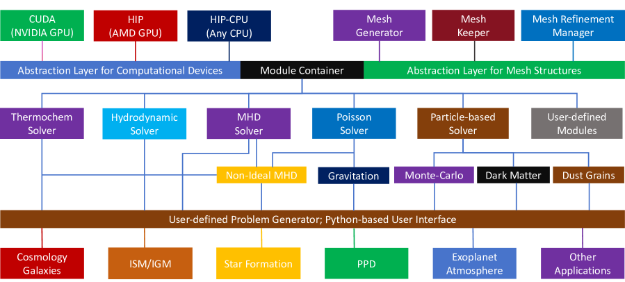
Figure 1: The overall structure of the Kratos code. Based on the abstration layer for computing devices and the abstraction layer for the mesh structures, the module container holds all capable modules for physical processes taking place in astrophysical simulations (hydrodynamic module elaborated in this paper; other modules will be described in forthcoming papers, L. Wang, in prep.). While complicated physical calculations can be constructed through the interactions of modules, a user interface (problem generator) handles the definition of intial, boundary, and in-simulation conditions. Such interface can also handle the initial conditions defined by a Python-based interface. Actual astrophysical objects and processes are simulated based on all fundamental systems described above.

2.1 Abstraction layer for devices

In what follows, the paper use the term “host” to denote the hardware and operations on the CPU (including the RAM on the CPU side), and “device” for the hardwares, software interfaces, and instructions that are hetrogeneous to the CPUs (e.g., GPUs; the term “GPU” will be used to denote all hetrogeneous devices with similar architechtures in what follows). On the contemporary high-performance and consumer-level computing markets, there have already been multiple programming models available, which are usually specific to the manufacturers of devices. To extend the portability on various hardware and software platforms while maximizing the performance by keeping the code close to the hardware, Kratos decides to implement the computations and algorithms via a new pathway by formulating all device-side codes in the subset that is the intersection between HIP and CUDA syntaxes, avoiding the usage of any manufacturer-specfic device calls.

On the host side that dispatches data transfer and device function (namely “kernels”) launching, the interfaces could have subtle differences (e.g., cudaMallocHost versus hipHostMalloc for allocating non-pagable host memory spaces). To resolve similar issues, Kratos also holds an abstraction layer on both host and device sides. This abstraction layer is implemented as a C++ class, containing the following ingredients that encapsulate the differences in syntax across various programming models:

• Initialization and finalization (destruction and resource release) for device enviroments;

• Device dispatching that assign a specific device to a CPU process;

• Fundamental attributes, including __global__, __host__, __device__ etc., which are commonly used in almost all relevant programming models, including CUDA and HIP;

• Directives related to shared memory on the device side;

• Application interfaces, including memory space allocations and de-allocations, host-device data transfer and copy procedures, calls of device calls (namely “device kenel launching”), and GPU stream and event operations.

All nuances comparing different programming models are absorbed by the abstraction layer, which assures Kratos to be compiled and run on different platforms without any modifications to the code. It is noticed that the intermediate layers have been introduced to models other than HIP and CUDA, including oneAPI (Intel, 2025) and OpenCL 3.0 (The Khronos Group, 2024). Equipped with encapsulation models such as chipStar , codes based on HIP can also be compiled and run on systems that are compatible with oneAPI and OpenCL3.0. What is more, using the open source library HIP-CPU that emulates GPUs via the TBB (thread building block) library, Kratos simulations can also be conducted using CPU with various architechtures that are compatible with TBB, including x86, ARM, and RISC-V.

2.2 Multiprocessing communication model

Kratos can be operated on multiple devices in parallel, and the code design requires that each device is controlled and managed by one host-side process. Data transfer among devices and processes are handeled by the communication module, which is established on the MPI (message passing interface) by default, while other implementations are also possible. It is worth noting that several maufacturers have introduced “device-aware MPI”, which allows direct transfers of device-side data without passing through the host-side memory. In general, however, Kratos does not always utilize this “device-awareness” MPI feature, because of the absence of “streams” in the MPI interfaces disables asynchronous communication (e.g. NVIDIA, 2025a).

Kratos employs a unified and encapsulated multiprocessing communication module, which adopts the standard MPI implementation as its default “backend,” adhering to version 3 of the standard. The module interfaces are largely similar to the MPI API in the C programming language, with an extra feature to optimize device-to-device communications: interfaces such as non-blocking send and receive operations are designed to accept device streams as arguments. This allows a communication task to be queued on a specific device stream, ensuring the correct handling of data dependencies and executaion sequence. These operations inevitably involves data transfer between host and device memories, which causes extra time consumption of data transfer. The introduction of device stream, however, enables the procedure pattern that allows the data transfer to take place following the correct sequence after all prerequisite computations are acompished. By properly design the pattern of communication procedures, Kratos generally attempts to maximize the efforts of “hiding” the communication operations behind the computations, and thus improving the overall performance of multi-device computation. Note that such communication feature is unlikely to be implemented even with the device-aware MPI (such as the “CUDA-aware” or “HIP-aware” MPI implementations that allow direct communications between device-side memory spaces), due to the absence of device streams in device-aware MPI API parameters. Details of the design for asynchronous communications utilizing streams are described in the explanation of each model, including the standard hydrodynamic module elaborated in §3.

The special communication module requires host-side buffers for proper data transfer, which are designed to be allocated on the first invocation. Capacities of these buffers are given by multiplying the requested size by a safety factor, which is typically around $\sim 1.2$. This factor has been found to be effective in the majority of multiple scenarios, although it should be noted that the optimal value may differ depending on the specific application requirements. These buffers are intentionally retained rather than being released back to the system, unless the subsequent requests for buffer sizes exceed their current capacity (when the original buffer is released and replaced with a newly allocated one), or until intentional de-allocation (e.g., one simulation as a whole comes to an end). Note that, although the hydrodynamic solver described in this paper does not involve variable buffer sizes, this feature is still required by other modules (especially particle modules) elaborated in following papers. This design choice minimizes the time-consuming overhead of buffer allocation and deallocation, thereby maintaining a clean and efficient runtime environment.

2.3 Mesh manager

2.3.1 Mesh tree and refinement

Kratos utilizes $2^{d}$-trees to manage its structured mesh, where $d\in\{1,2,3\}$ (thus octree in three dimensions, quadtree in two dimensions, and binary tree in one dimension). The trees fulfill dual roles: (1) to identify the spatial configuration of the sub-grids, and (2) to facilitate the allocation of geometry necessary for mesh refinement. Each node within this tree (not to be confused with the server node that denotes a single set of computer) referred to as a “block”. These blocks are the foundational elements that collectively compose the entire mesh, covering the entire domain of the simulation.

Based on the tree structure, mesh refinement is implemented for Kratos. Each block is represented by a node in the tree. Once a block is to be refined, it is replaced by $2^{d}$ blocks that have doubled resolution and halved size. When the number of refinement level $L$ is greater than one, the $2^{d}$-tree refinement scheme is carried out recursively, with an extra procedure adding prospectively extra refinement regions to guarantee that the absolute value of the difference in $L$ is no more than one for neighboring blocks.

The tree structure is organized by the C++ standard template library (STL) member std::map with the four-integer key values allocated in lexicographical order. These four-integers, indicated as $\{I,J,K,L\}$, define the “block indices”: the first three ($I,J,K$) stand for the logical indices of the block, and the $L$ for the refinement level (the coarsest level has $L=0$). When launched in parallel, each process holds a copy of the basic tree that holds the key values and communication information (including the identity number and the process rank number) of all blocks, while the detailed geometry data are only filled into the nodes that are held by the current process. This approach guarantees that all neighbors of every block can be easilily identified for communication purposes, while the tree size and communication costs are minimized when the tree is updated.

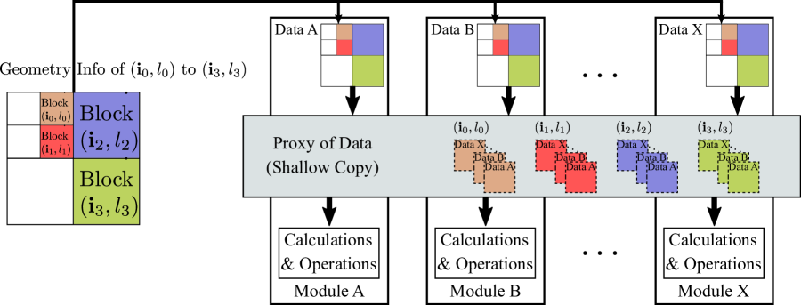
Figure 2: The method that Kratos handles the interaction of different physical processes via sharing the data held by modules. An instant data structure, encapsulating the shallow copy of all data needed held by all releva modules, is created as a data proxy right before the launching of each GPU job conducting the calculations.

2.3.2 Job dispatching and load balancing

When Kratos simulations are carried out on multiple devices, the computation load are dispatched to every device involved based on the mesh tree stucture. The job dispatching is managed by the load balancing module, which requires a scheme that maps the blocks distributed in the $d$-dimensional space onto a one-dimensional line segment. Using this mapping scheme, blocks are eventually distributed on the computing devices using the device number, either evenly or by a user-defined array of weights that takes other factors into account (e.g., the actual computing capability of each device). Although Kratos allows users to enroll their own implementation, by default, there are two different load balancing module that can be selected from.

The first is the row-filling scheme, which maps the $(I,J,K)$ block indices onto one dimension lexicographically. When the $2^{d}$-tree mesh refinement is applied, the simple row-filling scheme is applied to the blocks in the refined region, and replace the “original” coarse block in-place. The row-filling scheme addresses simulations in simple geometric layout with efficiency very close to optimal schemes, and suits several situations even better than other schemes when the row-filling scheme minimizes cross-process data dependencies (e.g., in simulations with plane-parallel ray tracing).

The second method is based on fractal space-filling curves, which naturally resolves the ordering of the refined region, since these curves can be generated recursively to a finer level once refinement is applied. Among the possible selections, the Hilbert curves ususally performs better for several reasons. The Hilbert curves are 2-based, in contrast to some other famous choices (e.g., the 3-based Peano curves), which maximizes the flexibility of the system. In addition, the Hilbert curve guarantees that the neighbors on the mapped one-dimensional space are also neighbors in the $d$-dimension space, which excels over other possibilities e.g. Z-ordering curves. To maximize the flexibility, Kratos also allows users to adopt their own rules for generating space-filling curves under the Lindenmayer System (L-system for short), and the default rules for Hilbert curves are also implemented under the L-system for 2D and 3D, respectively. In 3D, the L-system for Hilbert curves reads,

$$\begin{split}&X\rightarrow\wedge<XF\wedge<XFX-F\wedge>>\\ &\qquad\qquad XFX\&F+>>XFX-F>X->\ ;\\ &X\Rightarrow\text{Axiom (recursion interface)}\ ,\\ &F\Rightarrow\text{Move forward}\ ,\\ &+\Rightarrow\text{Yaw angle }+\pi/2\ ,\\ &-\Rightarrow\text{Yaw angle }-\pi/2\ ,\\ &\wedge\Rightarrow\text{Pitch angle }+\pi/2\ ,\\ &\&\Rightarrow\text{Pitch angle }-\pi/2\ ,\\ &>\Rightarrow\text{Roll angle }+\pi/2\ ,\\ &<\Rightarrow\text{Roll angle }-\pi/2\ .\end{split}$$ (1)

The application of space-filling curve load balancing will presented when illustrating the examples of hydrodynamics (§4.6).

2.4 Modules and module manager

Physical processes within a simulation are computed by specialized physical modules managed by the module container, which in turn relies on the data provided by the mesh manager. Unlike most other simulation systems, the relationship between the module container and the mesh manager is unidirectional in Kratos: the mesh does not hold any data or information about the modules, while the physical modules extract the necessary geometric data from the mesh to perform their calculations. When simulations are distributed across multiple devices, inter-block communication often becomes necessary for different physical modules to function effectively. Since each module may have unique communication requirements and patterns, the modules handle all related data and communication procedures independently. The data needed for these computations is stored within the modules themselves. This approach maximizes the flexibility of Kratos, which allows it to work as a code defined fully by the modules involved–for example, although hydrodynamics is the foundation of many modules, Kratos can still be a radiative transfer code that is totally irrelevant to the dynamics of fluids (H., Yang and L. Wang, in prep.).

In scenarios where data must be shared among multiple modules, explicit specification of data coupling is employed, facilitated through a data proxy scheme. This scheme involves creating a “shallow copy” of the data, which includes only the essential geometries and pointers to the GPU memory, on the CPU side before the module is executed on the GPU side. This method is depicted in Figure 2, and the implementation details of the modules will be discussed within the context of the modules themselves,providing a clearer understanding of how they operate and interact within the system.

The modules included with Kratos are intentionally crafted to be user-accessible for modification and expansion. The typical approach to extending their functionality is through inheritance, where users create custom classes by inheriting from the base default C++ class and overriding the relevant member functions. However, it is important not to implement this overriding using runtime polymorphism via virtual functions in C++: the usage of virtual tables can often lead to significant performance degradation on most heterogeneous devices, with various tests indicating a decrease in performance by more than one order of magnitude (not detailed in the current paper). Moreover, there is generally no practical need for runtime polymorphism in simulations,as the methods and algorithms used are typically predetermined. Consequently, Kratos opts for a different strategy, the compilation-time polymorphism through template metaprogramming. This approach utilizes the Curious Recursive Template Pattern (CRTP; see also Coplien 1995), which is based on F-bounded polymorphism (see Canning et al., 1989). By employing this pattern, Kratos can achieve the desired flexibility and customization without incurring the performance penalties associated with runtime polymorphism, thus ensuring that the modules remain efficient and effective for simulation tasks.

3 Hydrodynamics: the example and foundation of many modules

Figure 3: Scheme for one hydrodynamic cycle in Kratos, showing the parallelization pattern and the interface calls for data exchange. Each “rank” denotes a process, typically controlling one GPU, on which the calculations for multiple blocks are conducted. Each row (labelled by the “Block $X$, Stream $s_{X}$” at the beginning of each row) denote the numerical processes of one block on the $2^{d}$-tree mesh, which are located on one GPU stream for proper data synchronizations. Different steps of the Godunov solver are marked by colors (red for the preparation of primative variabs, green for calculation the Riemann fluxes, and magenta for the updates of conservative variables), while the communication operations are marked with blue. Black solid blocks stand for the synchronizations of each stream, taking place within the calls of communication operations to minimize waiting and thus maximize the efficiency.

The default hydrodynamics module in Kratos is not only the first implemented example module, but also the most optimized one. It plays a pivotal role in Kratos, as hydrodynamics is a fundamental aspect of various astrophysical research disciplines. Moreover, it serves as the cornerstone for numerous other modules and applications, such as magnetohydrodynamics, reacting flows, radiative hydrodynamics, and cosmology, among others. While detailed discussions of these modules and applications will be presented in subsequent papers, the focus of this work is to delineate and clarify the adaptations and optimizations made for heterogeneous devices. These optimizations are also the methodological foundation for the forthcoming studies.

The default hydrodynamic module is constructed within the Godunov framework, solving the Euler equation on descrete mesh,

$$\begin{split}&\partial_{t}\rho+\nabla\cdot(\rho\mathbf{v})=0\ ;\\ &\partial_{t}(\rho\mathbf{v})+\nabla\cdot\left(\rho\mathbf{v}\mathbf{v}+p\mathbf{I}\right)=0\ ;\\ &\partial_{t}\epsilon+\nabla\cdot\left[\left(\epsilon+p\right)\mathbf{v}\right]=0\ ,\end{split}$$ (2)

where $\rho$, $p$ and $\mathbf{v}$ are the fluid mass density, pressure and velocity, $\epsilon=\epsilon_{\rm g}+\rho v^{2}/2$ is the total energy density ($\epsilon_{\rm g}$ is the gas internal energy density), and $\partial_{t}$ denotes time derivatives. The solution procedures can be broken down into three key “sub-modules”: (1) the slope-limited Piecewise Linear Method (PLM) reconstruction, (2) the Harten-Lax van Leer with contact surface (HLLC) Riemann solver, and (3) the Heun time integrator, which is one of the second-order Runge-Kutta methods. When mesh refinement is employed, it is crucial to implement specialized schemes at the boundaries between finer and coarser mesh levels. The algorithms that govern the fluxes across cell surfaces are mathematically equivalent to those found in most existing computational fluid dynamics codes, as referenced in (Toro, 2009). However, to achieve optimized performance, it is essential to tailor these algorithms specifically for heterogeneous devices via re-arranging the sub-modules and schemes summarized in Figure 3. The synchronization calls of streams, which mark and guarantee that all operations are finished in sequence prior to the call on the same stream, are “postponed” to the communication. Because there are no dependency among different streams until synchronizations, such pattern allows the actual data transfer (from the GPU to the CPU side, and from one process to another) to take place in the background while the GPU is handling the prerequisite calculations for other blocks. In this way, a relatively large fraction of the communication costs are hidden behind the computation, so that the communication time is minimized. Detailed elaborations of more optimizations will follow in the subsequent discussion.

3.1 Variable conversion and boundary conditions

The default Riemann solvers in Kratos hydrodynamics work with primative variables–for hydrodynamics, the variable set contains $(\rho,p,\mathbf{v})$. As the conservative variables are the basic ones whose evolution is calculated on each step, conversion from conservative to primative variables needs to be calcualted first. The length of timestep $\Delta t$ is also calculated in the meantime of such variable conversion based on the Courant-Lewvy-Freidrich (CFL) conditions, which is conducted only on the first substep when the time integrator adopts a multi-step method.

If a Godunov algorithm has $n$th-order spatial accuracy, the reconstruction step will require $n$ cells on both sides for each cell interface. The consistency of calculations require primative variables to be available in the ghost zones, which form “buffer layers” surrounding blocks. This paper refers to the schemes of setting physical variables in the ghost zones as “boundary conditions”, which include both “physical boundaries” (p-boundaries) for the actual boundary of the whole simulation domain, and “communication boundaries” (c-boundaries) for the interfaces between neighbouring blocks.

3.1.1 Physical boundary conditions

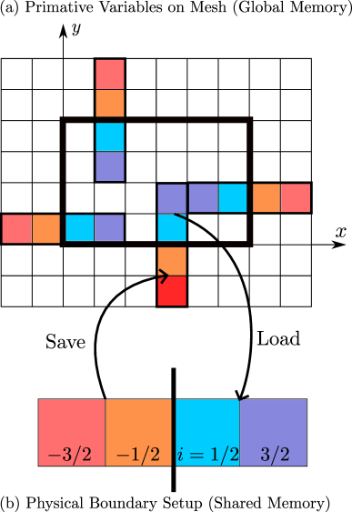
Figure 4: Boundary condition methods for hydrodynamics, showing four normal columns as examples to illustrate how Kratos rotate the normal columns to the $x$ direction to unify the methods on the interfaces of block boundaries. Colors indicate the corresponding cells before and after the rotations.

Kratos allows users to enroll their own p-boundary conditions to accommodate for the actual situations of astrophysical simulations. Note that when periodic boundary conditions are applied to the domain, the domain boundaries become c-boundaries instead. On the programming side, the p-boundary module in Kratos conducts proper manimupations including the reflection and alternation of coordinate axes during the loading and saving stages of the variables inside and near the p-boundaries, so that all actual p-boundary operations are mathematically equivalent to dealing with the boundary condition in the $x$-direction on the left, as is shown in Figure 4.

Users can set different p-boundaries on different sides. There are three default options, which are expressed with the indexing for the left $x$-boundary (see also Figure 4; integers are used for cell faces, and half integers for cell centers):

1. Free boudnary: $q_{-i-1/2}=q_{1/2}$;

2. Outflow boundary: $q_{-i-1/2}=q_{1/2}$,
   but $v_{x,-i-1/2}=\mathrm{min}\{v_{x,1/2},0\}$;

3. Reflecting boudnary: $q_{-i-1/2}=q_{i+1/2}$,
   but $v_{x,-i-1/2}=-v_{x,i+1/2}$.

Here $0\leq i\leq n_{\rm gh}-1$, and $n_{\rm gh}$ corresponds to the spatial order of the reconstruction. Note that the transform automatically rotates the normal component of velocity (pointing inwards) into $v_{x}$, and rotates $v_{x}$ back to the desired component and direction after the boundary condition algorithms are applied.

3.1.2 Communication boundaries

Figure 5: Restriction and prolongation operations near the block refinement interface. Colors are used to mark the corresponding relations across the interface separating coarser (left) and finer (right) blocks. The prolongations are computed on the coarser side, and the $x-$ derivatives $q_{x,I,J}$ are calculated using minmod slope limiter in a pattern indicated on the corser mesh (derivatives along other directions can be obtained similarly).

When a simulation domain is partitioned into multiple blocks, it is crucial to establish consistent c-boundaries for the physical variables across these blocks. In the context of hydrodynamics, c-boundaries pertain only to the interfaces between blocks, or block faces. The communication patterns between these blocks are relatively simple and direct, especially when there is no mesh refinement involved. To further reduce the time spent on communication, Kratos incorporates an additional optimization technique, handling data transfers within the same device by directly writing the ghost zone data to the destination, bypassing the usual communication interfaces as described in section §2.2.

Kratos hydrodynamics relies on the the $2^{d}$-tree method also for its mesh refinement, which plays a pivotal role in managing the c-boundaries at the interfaces between refined and coarser meshes. The general mechanism of c-boundary mesh refinement is presented in Figure 5, which illustrates the prolongation and restriction schemes for primitive variables near the block boundaries that separate blocks of different levels. The restriction operations, which involve transferring data from finer to coarser grids, are simply executed by performing volume-weighted averages. Conversely, the prolongation step, which interpolates data from coarser to finer grids, requires a more nuanced approach. This step must comply with the TVD (total variance diminishing) condition to prevent numerical instabilities that can arise from the interpolation process. The minmod function,

$${\rm minmod}(a,b)=\begin{cases}&a\ ,\quad|a|<|b|\ {\rm and\ }ab>0;\\ &b\ ,\quad|a|\geq|b|\ {\rm and\ }ab>0;\\ &0\ ,\quad ab<0\ ,\end{cases}$$ (3)

is used to evaluate the derivatives in the slope-limited piecewise linear method (PLM). The minmod function is crucial for maintaining the stability and accuracy of the simulation by limiting the slope of the reconstructed variables, thus preventing oscillations that could lead to unphysical results.

The communication pattern in Kratos hydrodynamics is designed in a specific sequence to ensure the consistency and efficiency of computations:

1. Finishing all communication operations that are not directly related to cross-level block boundaries, to prepare for necessary data for prolongation;

2. Conducting prolongation calculations on the coarser blocks over all cross-level boundaries before sending the prolongated data to finer blocks, as the coarser blocks have complete information required;

3. Calculating the fluxes on all blocks (see §3.2);

4. Sending the flux information at the cross-level block boundaries from the finer side to the coarser side, and sum up the fluxes accordingly to obtain the fluxes that are actually adopted on the coarser side at the cross-level interface, so that the conservation laws are maintained at the c-boundaries.

3.2 Flux calculation

Almost all hydrodynamic methods in the FVM category have the most time-consuming part on the computations of fluxes for hydrodynamic variables. The efforts of improving the performance of hydrodynamic simulations should focus on the optimization of flux calculations.

3.2.1 Shared memory utilization

The access of data in the global device memory (“global memory” hereafter; not to be confused with the system memory on the CPU side) suffer from excessive latency (typically equivalent to $\sim 10^{2}$ or even more clock cycles for the awating computing units) on hetrogeneous devices. This issue becomes even worse for transposed data access when calculating the fluxes along the directions perpandicular to the $x$-axis. To reduce the cost of memory access, almost all contemporary hetrogeneous computing devices and their corresponding model have an important feature, named “shared memory”, that can significantly improve the performance. Shared memory indicates memory spaces that are typically allocated on the L1 cache of stream multiprocessors (SMs). Such memory spaces are equivalently fast as L1 when accessed by computing units, while the data flow can be controlled by the programmer, in contrast to the ordinary L1 cache spaces that are controlled by the default dispatcher.

Proper utilization of the shared memory is a necessity for maximizing the performance of flux calculations, minimizing the frequency of accessing the data staying in the global memory by adequately coordinating the data flow. The reconstruction step, regardless of the actual algorithm, obtains the physical variables on both sides of an interface separating neighbouring cells. The $l$th order reconstruction method will require data from $2(l+1)$ cells for one interface, and in turn, data in one cell (not in ghost zones) will be read by the reconstruction of $2(l+1)$ interfaces. These data dependencies, illustrted in Figure 6, clearly indicates the dispatching procedures for reconstruction, to load the row of related data into the shared memory first, and then conduct subsequent calculations using the data and space in the shared memory.

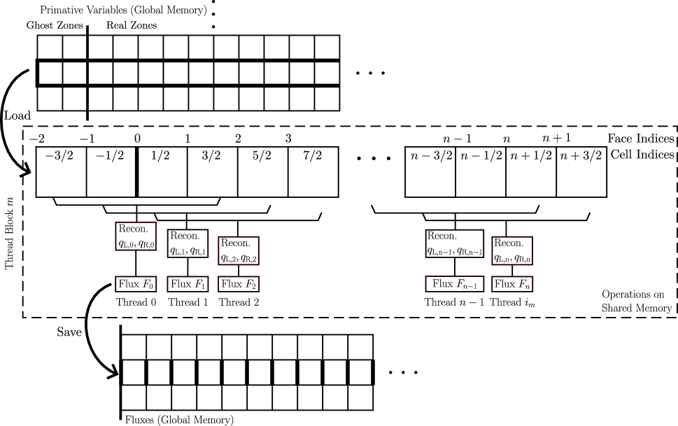
Figure 6: Patterns of calculating the fluxes for hydrodynamics, illustrating the utilization of shared memory. All processes within the middle dashed box use the shared memory instead of the global memory, as the memory-related operations are frequent, and the data in each cell is typically used many times by multiple threads (indicated by the braces and blocks in the middle box).

3.2.2 Mixed-precision methods

In the Kratos framework, the hydrodynamics module is implemented via a mixed-precision approach, a feature that ensures both accuracy and computational efficiency. This methodology defines a float2_t data type (double precision by default, typically represented by 64-bit floating-point numbers), to maintain the conservation laws of hydrodynamics with machine-level precision for conservative variables, encompassing mass density, energy density, and momentum density. Meanwhile, the hydrodynamics module approximates the fluxes of these conservative variables using approximate Riemann solvers, a common practice in most of the finite volume hydrodynamics simulation codes. Therefore, employing full double precision methods for these calculations is not mandatory, provided that numerical stability is guaranteed. To this end, the hydrodynamics module opts for the float_t data type, which defaults to single precision (typically represents 32-bit floating-point numbers), for the reconstruction schemes and the approximate Riemann solvers. This approach ensures that the conservation laws are upheld to the precision inherent in float2_t, while also maintaining physical reliability by holding the conservation laws.

It is worth noting that, through the appropriate selection of compilation options, the data types float_t and float2_t can be mapped to either single or double precision, offering flexibility in the precision requirements of the simulation. This feature is useful in scenarios where double precision is mandated, especially when using devices that have comparable computational capabilities for both single and double precision operations (e.g. the Tesla series of computing GPUs).

The process of resolving fluxes is generally broken down into two main steps. The initial step involves the slope-limited PLM reconstruction, which is easily executed in single precision. However, it is crucial to use the cell center distance, $\Delta x$, directly in the denominator for numerical derivatives to avoid significant errors that can arise from large number subtractions, a phenomenon known as “catastrophic cancellation”. The subsequent step involves approximately solving the Riemann problem, a process similar to the methods detailed in Toro (2009). The HLLC solver is used as a default example, where the contact surface speed $s_{*}$ is the crucial value,

$$s_{*}=\dfrac{[p_{R}-\rho_{R}u_{R}(s_{R}-u_{R})]-[p_{L}-\rho_{L}u_{L}(s_{L}-u_{L})]}{\rho_{L}(s_{L}-u_{L})-\rho_{R}(s_{R}-u_{R})}.$$ (4)

It is noted that, when $|s_{i}-u_{i}|\ll|u_{i}|$ ($i\in\{L,R\}$) for either left (L) or right (R) states, the reliability of the equation for $s_{*}$ is compromised. Numerical tests have shown that single precision calculations can lead to more instances of catastrophic cancellations and unreliable results, or even vanishing denominators in the equation for $s_{*}$. To mitigate this, subtraction-safe modifications are implemented,

$$\begin{split}&\Delta s_{L}\equiv s_{L}-u_{L}=-c_{s,L}q_{i}\ ,\\ &\Delta s_{R}\equiv s_{R}-u_{R}=c_{s,R}q_{i}\ ;\\ &q_{i}=\left[1+\dfrac{\gamma+1}{2\gamma}\left(\mathrm{max}\left\{\dfrac{p_{*}}{p_{i}},1\right\}-1\right)\right]^{1/2}.\end{split}$$ (5)

leveraging the fact that $\Delta s_{L}$ is always negative and $\Delta s_{R}$ is always positive, which prevents catastrophic cancellations or vanishing denominators in eq. (4).

By applying a mixed-precision algorithm to the HLLC Riemann solver within the Kratos module, extensive testing has confirmed that the relative error remains below $10^{-3}$ when compared to the double precision version across the parameter space relevant to typical astrophysical hydrodynamic simulations (not shown in this paper). For direct tests against analytic solutions in shock tube scenarios as part of the Godunov solver pipeline, readers are directed to §4.1 for further details.

3.3 Time integrator

The time integrator is an independent sub-module within the hydrodynamic solver. By default, the time integration is conducted by the Heun method, one of the widely adopted second-order Runge-Kutta integrators, in which the “one-step integration” block is equivalent to the whole cycle described in Figure 3. One feature of the Heun method is that the integrated variables of the predictor sub-step (also known as the intermediate sub-step) directly enters the results of the whole step with weight $1/2$, which requires that the predictor sub-step results should be recorded with the same precision as the whole step.

When the memory occupation is a concern, one can also select the memory-optimized second order van Leer integrator. This integrator can store the prediction sub-step results in the space for primative varibales with reduced precision, since the van Leer integrator does not1 directly use the prediction step in the final results. Such approach saves up to $\sim 1/3$ of the device memory for hydrodynamics, while keeping the conservation law up to the full machine accuracy.

4 Verifications and performance tests

Several fundamental and standard tests of the Kratos code are presented in this section. Some of them are not only verifying the correctness and robustness of the algorithms involved, but also used as the opportunity of testing the performance for the computing speed.

4.1 Sod shock tubes

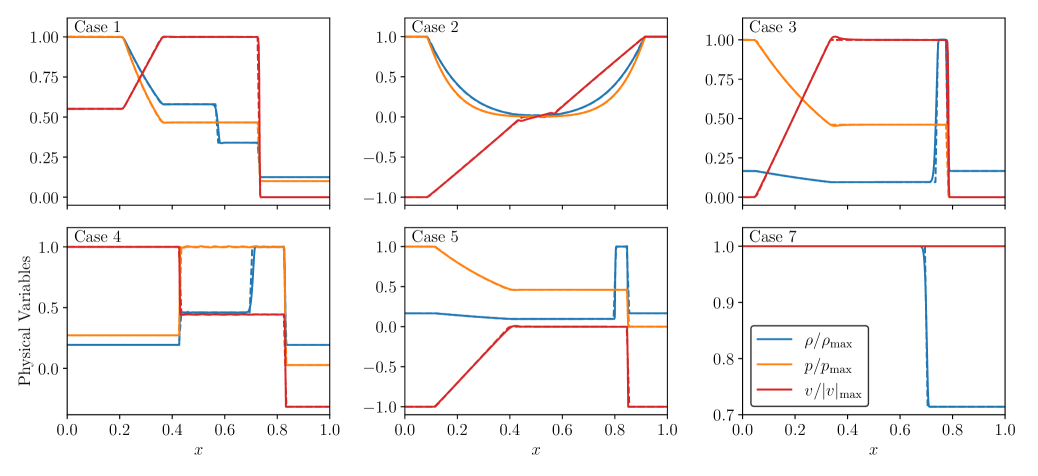
Figure 7: The one-dimensional tests of Sod shock tubes, showing the results of cases 1–5 and 7 in Toro (2009) using the original setups and parameters. The exact semi-analytic solutions are indicated by dashed lines, in the same color for the corresponding physical quantities of Kratos numerical calculation results. All calculations in these tests use mixed precision methods.

The shock tube problem serves as a canonical benchmark for assessing the accuracy and robustness of hydrodynamic solvers, as well as the integrity of the overall simulation infrastructure. While it is acknowledged that the presence of expansion fans within the shock tube scenario precludes the existence of exact analytic solutions, the derivation of semi-analytic solutions remains a feasible and straightforward endeavor. In this context, we present a series of simulation results, depicted in Figure 7, which correspond to a variety of initial configurations. These configurations are drawn from the standard test problems outlined in (Toro, 2009). It is important to highlight that the mixed precision HLLC approximate Riemann solver has been deliberately selected for these tests, yielding results that demonstrate a consistent alignment with the analytic solutions across all examined cases.

Furthermore, we have extended the standard Sod shock tube tests, which traditionally consider fluid motion along the $x$-axis, by conducting additional tests that interchange the axes of fluid motion. The findings from these modified tests are found to be identical to those obtained from the standard x-axis tests. This congruence underscores the versatility of the finite volume scheme employed, which facilitates the calculation of fluxes through the pre-update primitive variables, thereby highlighting one of the key advantages of this approach.

4.2 Double Mach reflection test

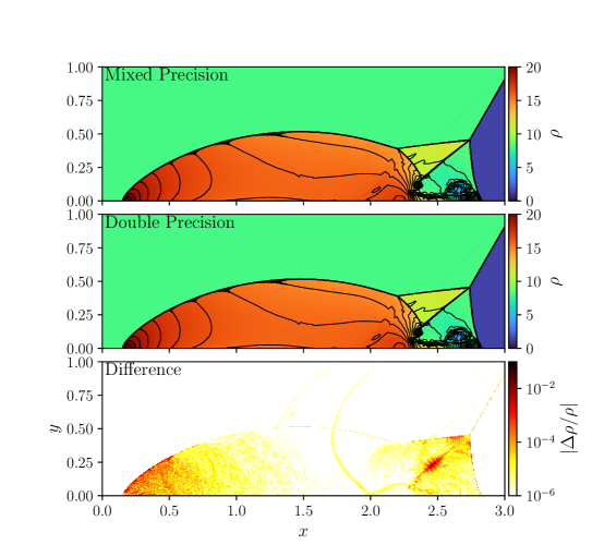
Figure 8: Results of double Mach reflection tests, using mixed precsision (top panel) and full double precision (middle panel) methods. The 30 contour lines starting from $\rho=1.73$ to $\rho=2.1$ are spaced evenly in $\rho$, indicating almost identical patterns on these panels. The bottom panel illustrate the relative differences of mass density comparing the top two panels.

The double Mach reflection tests, as canonical benchmarks for hydrodynamics simulations, is employed to rigorously evaluate the precision and dependability of simulation frameworks. This test, initially formulated by Woodward & Colella (1984), presents a scenario where a Mach 10 shock wave impinges upon an inclined plane, leading to complex interactions with the reflected shock wave and the emergence of a triple point. These dynamics yield a spectrum of hydrodynamic phenomena, including shock discontinuities and the generation of a high-velocity jet. The intricate flow structures that result are instrumental in assessing a code’s capacity to accurately and robustly manage multi-dimensional discontinuities, particularly shock waves. For this test case, the initial conditions and boundary specifications are derived directly from Woodward & Colella (1984), with a slightly expanded spatial domain of $(x,y)\in[0,4]\times[0,1]$ and a resolution of $4096\times 1024$. To accurately simulate the propagation of the inclined incident shock, a time-dependent boundary condition is implemented along the upper boundary, leveraging the p-boundary condition framework detailed in Section 3.1.1.

Figure 8 illustrates contour plots superimposed on a colormap representation of the solution at $t=0.2$, juxtaposing mixed and full-double precision methods under identical conditions. It is evident that the two algorithms, despite their differing precision levels, exhibit near-perfect convergence, with the maximum relative discrepancy not exceeding $\sim 10^{-2}$ as indicated by the mass density. These outcomes closely mirror Figure 4 in Woodward & Colella (1984), with the distinction that our results showcase sharper shock fronts attributable to higher-order spatial accuracy and a significantly enhanced resolution. In comparison with the analyses presented in Gittings et al. (2008) and Stone et al. (2020), the carbuncle-like instability near the jet’s head is not entirely mitigated by the HLLC solver, which is known to introduce less numerical diffusion than the HLLE solver. Nevertheless, the near-identical behavior between mixed and double precision results at the jet head further substantiates the validity and robustness of the mixed precision solver.

The performance assessments based on the double Mach reflection problem are summarized in Table 1, with $10^{8}-10^{9}$ cells per second computational efficiency per device on contemporary GPUs. On GPUs for the consumer market (such as the NVIDIA RTX series and AMD 7900XTX), mixed precision calculations run at speeds comparable to the full single precision (around $\sim 70-80\%$), and are almost $\gtrsim 5-7$ times faster than the full double precision runs. These speeds are not proportional to the theoretical single and double precision floating point computing efficiency of GPUs, as deeper profiling and timing tests of Kratos reveal that, even with relatively thorough optimization on the data exchange and cache or shared memory utilization (§3.2.1), a significant fraction of computing time is still occupied by the data exchange between the global graphics memory and the cache (not shown in this paper). On computing GPUs (such as Tesla A100 and MI100) with enhanced double precision performance, the mixed precision methods do not exhibit considerable advantages compared to full double precision. The compatibility of Kratos on x64 and ARM CPUs is also confirmed and illustrated in Table 1. It is noted that the performance with HIP-CPU per physical CPU core are far below the other CPU codes on same devices, by approximately $\sim 3-7$ times (e.g. Stone et al., 2020). Because the HIP-CPU actually emulates GPUs using non-optimized patterns (including the implementation of multi-threading dispatching algorithms and launching overheads), Kratos on HIP-CPU is implemented primarily for compatibility and code devloping (especially debugging) considerations, rather performance purposes.

Table 1: Performance test results of double Mach reflections.

Programming Models	Computing Speed with Precision
and Devices	($10^{8}{\rm\ cell\ s}^{-1}$)
	Single	Mixed	Double
HIP-CPU∗
AMD Ryzen 5950X†			0.15
Qualcomm Snapdragon 888∗∗			$0.0037$
NVIDIA CUDA
RTX 2080TI	9.2	6.9	0.93
RTX 3090	14	10	1.4
RTX 4090	21	16	2.9
Tesla A100	16	14	8.3
AMD HIP
7900XTX	8.9	7.7	2.8
MI100	8.2	6.8	3.0

Note. — Presenting the average over $10^{2}$ steps. All tests cases are in 2D. Detailed setups see §4.2.

*: Only double precision results are concerned, as modern CPUs have almost the same single and double precision computing speeds.

$\dagger$: Utilizing all 16 physical cores.

**: Using termux (https://termux.dev) on Android operating system, utilizing one major physical core. Compile-time optimization are turned off because of the software restrictions of TBB on ARM CPUs.

4.3 Liska-Wendroff implosions

Figure 9: The Liska-Wendroff implosion tests results, showing $t=0.045$ (upper row) and $t=2.5$ (lower row), comparing the mixed precision (left column) and full double precision (right column) methods. Contours span from $\rho=0.35$ to $\rho=1.1$, spaced evenly by $\delta\rho=0.025$.

The Liska-Wendroff implosion test, as detailed in Liska & Wendroff (2003), serves as a benchmark for assessing the directional symmetry preservation of hydrodynamic simulation methods. This test is initiated with an initial condition that is similar to the Sod shock-tube scenarios, but with a diagonal orientation. A shock wave in the $\gamma=1.4$ gas is generated by applying an under-pressure region in the lower-left corner of the domain,

$$(\rho,p,\mathbf{v})=\begin{cases}&(0.125,0.14,0)\ ,\quad x+y<0.15\ ;\\ &(1,1,0)\ ,\quad\text{elsewhere}\ ,\end{cases}$$ (6)

which is then reflected by the bottom and left boundaries. The initial discontinuity is set at a $\pi/4$ angle to the coordinate axes, with reflecting boundary conditions applied on all sides. The reflected shocks interact with other discontinuities, including contact discontinuities and additional shocks, leading to the development of finger-like structures via the Richtmeyer-Meshkov instability along the direction of the initial normal vector. The direction of the jet serves as a critical indicator of whether the simulation method maintains reflective symmetry to machine precision. In some early hydrodynamic simulation systems that employed directionally split algorithms, the jet’s impact at the lower-left corner might not align precisely with the corner, resulting in vortices that deviate significantly from the diagonal line. This deviation highlights the importance of directional symmetry in accurately capturing the dynamics of the system.

Figure 9 illustrates the density profiles at $t=0.045$ and $t=2.5$, comparing the results obtained from mixed precision and double precision methods. The double precision results exhibit good symmetry across the diagonal at $t=2.5$, with the exception of the lower left corner, which is prone to strong instabilities and turbulence. The mixed precision results also maintain a large degree of reflection symmetry; however, the wake of the jet-induced vortices shows a noticeable departure from perfect symmetry when visualized with contour plots. It is important to note that the last significant digits in floating-point calculations on GPUs are not guaranteed to be identical for both single and double precision, and the associated errors are inherently undetermined (e.g. NVIDIA, 2025b). Amplified by chaotic motions, such random errors eventually lead to the symmetry breaking. Before employing mixed precision methods in practical applications, it is crucial to ascertain whether strict reflection symmetry is necessary. Additionally, it should be recognized that this type of discrete symmetry breaking, caused by slightly differing results from separate calculations, does not affect continuous symmetries, such as the conservation laws of mass and momentum.

4.4 Kelvin-Helmhotz instabilities

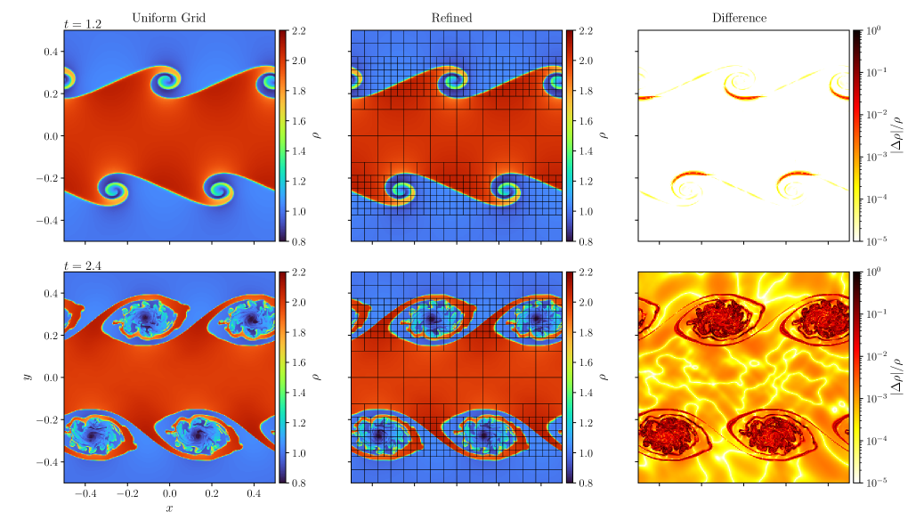
Figure 10: The Kelvin-Helmhotz instability tests results, comparing the $t=1.2$ (upper row) and $t=2.4$ (lower row) for the uniform grid (left column) and SMR (middle column) results for the relative difference (right panel) in mass density. The block boundaries are indicated in the panels for the SMR simulation, showing the mesh refinement results (note that each block has the same number of cells).

The tests on Kelvin-Helmhotz instabilities are one of the “standard procedures” for many numerical simulation systems. Such tests, similar to Lecoanet et al. (2016), are conducted on $\gamma=1.4$ gases with initial conditions,

$$\begin{split}&\rho=\rho_{0}+\Delta\rho\tanh\left(\dfrac{|y-y_{0}|}{L}\right)\ ,\\ &v_{x}=v_{x0}\tanh\left(\dfrac{|y-y_{0}|}{L}\right)\ ,\\ &v_{y}=v_{y0}\cos(kx)\exp\left[-\dfrac{(y-y_{0})^{2}}{2\sigma^{2}}\right]\ ,\end{split}$$ (7)

where $\rho_{0}$, $v_{x0}$ and $v_{y0}$ are the reference values for density and $x,y$ velocity components, $\Delta\rho$ is the difference in density across the shearing layer with thickness $L$, $k$ is the velocity perturbation wavenumber, and $\sigma$ is the thickness of the perturbation region. This paper chooses the parameters $L=0.01$, $y_{0}=0.25$, $\rho=1.5$, $\Delta\rho=0.5$, $v_{x0}=0.5$, $v_{y}=0.01$, $k=4\pi$, and $\sigma=0.2$. These 2D simulations are carried out within a spatial domain of ${x,y}\in[-0.5,0.5]\times[-0.5,0.5]$. The uniform grid simulations employ a resolution of $\Delta x=1/2048$ across the entire domain, whereas the mesh refinement approach ensures this resolution is maintained in the regions $|x|\in(3/16,3/8)$ through the application of two levels of static mesh refinement. Periodic boundary conditions are applied to the $x$ boundaries, and reflective conditions elsewhere.

The results of these tests are illustrated in Figure 10, which compares the outcomes from uniform grid simulations with those from simulations utilizing mesh refinement. At $t=1.2$, the upper row of the figure illustrates results that are nearly indistinguishable between the two methods, with a relative error not exceeding $5\times 10^{-2}$. The minor differences observed are primarily localized near regions of density discontinuities, likely due to subtle structural displacements. At $t=2.4$, the patterns remain largely consistent, yet the quantitative differences between the uniform grid and mesh refinement results are more pronounced, reaching up to $\sim 10^{-1}$. These discrepancies are also attributed to structural displacements, as evidenced by a direct comparison of the uniform grid and mesh refinement panels. It is important to note that simulations employing mesh refinement may still exhibit variations from those with high-resolution uniform grids, particularly in the damping of short-wavelength modes within unrefined, low-resolution areas. The kinetic diffusivity parameter, which is influenced by numerical methods, scales with $\eta\propto\Delta x^{2}/\Delta t$. This phenomenon has also been observed in various studies, and is further supported by the work of Stone et al. (2020).

4.5 Rayleigh-Taylor instabilities

Figure 11: The Rayleigh-Taylor instability tests, showing $t=2,3$ and $4$ results in three columns for the simulations on uniform grid (top row) and with SMR (bottom row). Similar to Figure 10, the block boundaries are indicated to illustrate the mesh refinement layouts.

The Rayleigh-Taylor instability (RTI) test, a standard benchmark for evaluating the efficacy of numerical methods in multi-dimensional hydrodynamics, is further detailed in e.g. Liska & Wendroff (2003) and Lecoanet et al. (2016). This test is useful for assessing how numerical schemes behave in the presence of complex fluid interactions. This test also examines the performance of the code under static mesh refinement, as the regions where significant hydrodynamic features are anticipated to emerge can be identified with relative ease a priori.

The simulated domain covers $(x,y,z)\in[-1/4,1/4]\otimes[-1/4,1/4]\otimes[-1/2,1]$ with $\gamma=1.4$ gas. While the uniform grid test employs a grid spacing of $\Delta x=1/256$, the mesh refinement scenario focuses on a refined region of $(x,y,z)\in[-1/4,1/4]\otimes[-1/4,1/4]\otimes[-1/2,1]$ to the second level, achieving a grid spacing of $\Delta x=1/1024$. Reflecting boundary conditions are implemented on all physical boundaries. Initially, the density is set to $\rho=2$ for $z>0$ and $\rho=1$ for $z\leq 0$. The pressure is determined based on the vertical gravitational acceleration $g_{z}=-0.5$ (negative indicating the downward direction of gravity), ensuring a hydrostatic equilibrium calibrated at $p_{z=0}=2.5$. An initial velocity perturbation is introduced as $v_{z}=10^{-2}\cos(\mathbf{k}\cdot\mathbf{x})$, where $\mathbf{k}\equiv(4\pi,4\pi,3\pi)$ represents the perturbation wavenumber.

The outcomes of the tests, encompassing mesh refinement conditions, are depicted in Figure 11, presenting a comparative analysis between simulations with and without mesh refinement at various evolutionary times. It is important to note that, due to the absence of explicit viscosity or surface tension, the emergent shear instabilities parasitic on the Rayleigh-Taylor instability patterns are theoretically expected to grow at nearly all wavelengths. The actual results are, therefore, affected by the numerical diffusivities, which are proportional to $\eta\propto\Delta x^{2}/\Delta t$. This leads to significant differences when comparing mesh refinement results with those obtained using low-resolution uniform grids. With equivalent resolution of $\Delta x=1/1024$ on the refined mesh, the non-linear fine structures are more pronounced due to reduced numerical diffusivities, while the overall “mushroom” structures remain quantitatively similar for both scenarios.

The performance metrics of Kratos in these tests are summarized in Table 2. As the Rayleigh-Taylor instability tests are conducted in 3D, the time consumption due to the flux calculations on the third dimension nominall reduces the speed (in cells per second) by around $\sim 1/3$ when compared to the 2D results in Table 1. One can also observe by comparing the single-device speed with dual-device speed (the first and second numbers of each data entry in the table) that the cross-device parallelization performance is good with two devices other than RTX 4090 (up to $\sim 90\%$ the theoretical performance). This indicates that the workflow design (see also §3 and Figure 3) is successfully optimizing out the communication overheads. When using the RTX 4090 GPUs, however, the scalability appears to be worse, as the high single-GPU performance partially fails the workflow in hiding the communication operations behind computations.

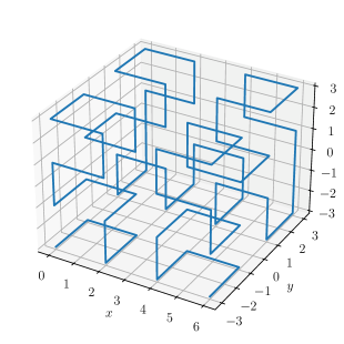
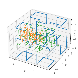
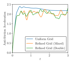
Figure 12: Results of the tests on colliding outflows and ambient gases, showing the mas density profiles at $t=1$ (top row) and $t=2$ (middle row) for low resolution ($\Delta x=1/32$; left column), SMR with mixed precision (equivalent $\Delta x=128$; middle column) and SMR with full double precsion (right column) cases. Block boundaries are indicated in related panels to illustrate the mesh layouts. The bottom row illustrates the Hilbert curves generated for the job dispatching and load balancing for the uniform grid (left panel) and SMR (middle panel) simulations, where the lines connecting blocks on different levels are shown in different colors, and cross-level connections are indicated by dashed lines. The evolution history for the acceleration on the central object of the three different simulations (lower right panel).

Table 2: Performance test results based on the Rayleigh-Taylor instability simulations.

Programming Models	Computing Speed with Precision
and Devices†	($10^{8}{\rm\ cell\ s}^{-1}$)
	Single	Mixed	Double
HIP-CPU
AMD Ryzen 5950X∗			(0.15, - )
NVIDIA CUDA
RTX 3090	(8.6, 14.7)	(6.2, 11.2)	(0.61, 1.1)
RTX 4090	(12.4, 17.7)	(10.1, 16.3)	(1.3, 2.4)
Tesla A100	(8.3, 14.6)	(8.3, 12.9)	(4.7, 8.2)
AMD HIP
7900XTX	(3.6, 5.7)	(3.4, 5.5)	(0.94, 1.86)
MI100‡	(3.7, -)	(3.6, -)	(2.1, -)

Note. — Presenting the average over $10^{2}$ steps. Results are presented as groups of numbers ($s_{1},s_{2}$), where $s_{1}$ is for the single-devicle speed, and $s_{2}$ for the dual-device one. All tests cases are in 3D (see §4.5).

$\dagger$: Some devices involved in Table 1 are not applicable in these tests.

*: Dual-device tests not applicable.

$\ddagger$: Tests are not conducted on dual-device MI100 systems due to technical restrictions.

4.6 Collidingas outflow and ambients

A traditional yet highly relevant scenario, which could showcase the performance and capabilities of the simulation, involves interactions between stellar outflows and ambient gas flows induced by the relative motion of stars and their surrounding medium. This scenario is not only of historical significance but also gains contemporary relevance in the dynamical studies of stars and compact objects, as highlighted in recent literatures (e.g. Li et al., 2020; Wang & Li, 2022).

These tests are conducted for $\gamma=1.4$ gas, within a cubic spatial domain defined by the coordinates $(x,y,z)\in[-1,7]\otimes[-4,4]\otimes[-4,4]$. At the left boundary along the $x$-axis, an inflow is introduced with a velocity of $v_{\rm in}=5$, a density of $\rho_{\rm in}=1$, and a pressure of $p_{\rm in}=1$. At the coordinate origin $(x,y,z)=(0,0,0)$, a spherical source with a radius $r=0.1$ is established to emit gas at a rate of $\dot{m}=13$ units of mass per unit time with a radial velocity of $v_{r}=10$. The outcomes of these tests are depicted in Figure 12, where three distinct cases are compared:

1. Uniform grid with $\Delta x=1/32$ with full double precise methods;

2. Refined grid with equivalent resolution $\Delta x=1/128$ within the $(x,y,z)\in[-1,3]\otimes[-1,1]\otimes[-1,1]$ region, using mixed precision methods (§3.2.2);

3. Same as 2, but using full double precision methods.

The comparisons are made at two temporal snapshots, $t=1$ and $t=3$. At $t=1$, the semi-quantitative similarities among the three cases are apparent. The first case lacks instabilities due to higher damping from lower resolution, while the latter two cases, by incorporating mesh refinement, display clear signs of growing instabilities. By $t=3$, the divergence between the latter two cases becomes more apparent, as evidenced in the lower-right panel illustrating the net acceleration. The reflection symmetry across the plane $y=0$ is broken in both refined cases, even with the utilization of full double precision, despite commencing from identical initial conditions that strictly maintain reflection symmetry. This asymmetry, as discussed in §4.3, originates from the intricacies of floating-point calculations on heterogeneous devices. With hydrodynamic instability modes unattenuated at higher resolutions, the disruption of symmetry and the ensuing chaotic turbulent evolution are anticipated phenomena.

The lower-left and lower-center panels in Figure 12 exhibit the application of Hilbert curves in scenarios with uniform and refined meshes, respectively. It is evident that with the L-system employed in the mesh refinement framework (§2.3.2), the Hilbert curve is properly generated within the refined region through recursion, and task distribution is executed accordingly. A few scalability tests are also carried out under this scenario, as summarized by Figure 13. Similar to the data presented in §4.5 and Table 2, the strong and weak scalings of Kratos on multiple devices is good when the single-device computation speed is relatively slow ($\lesssim 3\times 10^{8}$ cells per second per device), and the results start to deterioate with faster computing modes (e.g., mixed precision with RTX 4090) the issue of communication overhead (by “not perfectly hiding communication behind computation”). Because current consumer-level GPUs are disabled for the GPU-to-GPU direct commnunication functionality on the driver level, such deterioation is inevitable unless this restriction is removed. However, with the microphysics modules being introduced the deterioation of scalability is expected to be less apparent due to significantly higher local computing costs, especially when real-time thermochemistry is involved (in the forthcoming papers, L. Wang, in prep.).

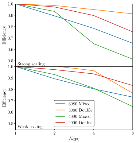
Figure 13: Scaling performance on multiple GPUs on different types of devices (RTX 3080 and RTX 4090), with mixed precision and full double precision methods respectively. Tests are based on the outflow–incoming flow interactions (see §4.6 and Figure 12). The upper panel shows the strong scaling (with the same total computation load), and the lower panel is for the weak scaling (with the same computation load per device).

5 Summary and forthcoming works

This paper describes the Kratos Framework, a novel GPU-based simulation system tailored for astrophysical simulations on heterogeneous devices. Kratos is designed to harness modern GPUs, providing a flexible and efficient platform for simulating a broad spectrum of astrophysical phenomena. It fundamental infrastructures relies on abstraction layers for devices, a multiprocessing communication model, and a mesh management system. These buildingblocks are designed for heterogeneous computing environments (especially GPUs) consistently, preparing for the supports for various physical modules, including hydrodynamics (which is elaborated in this paper), and thermochemistry, magnetohydrodynamics, self-gravity, and radiative processes in forthcoming papers.

Kratos is constructed for the CUDA, HIP and similar GPU programming models, employing abstraction layers to insulate algorithms from programming model disparities, thereby optimizing performance and ensuring compatibility across different GPUs without modifying the actual implementations of algorithms. The basic mesh structures of Kratos utilizes $2^{d}$-trees for structured mesh management, with mesh refinement implemented recursively. Job dispatching and load balancing, which can involve user-defined schemes, use Hilbert curves based on L-systems by default. Mesh structures are designed to be separated from physical modules, so that involving multiple physical modules can be naturally accomplished. The multiprocessing communication model are implemented for device-to-device communications that allows the GPU stream to be involved, thus optimized for the computation on systems equipped with consumer-level GPUs.

The hydrodynamics module of Kratos is constructed within the Godunov framework, and the default implementation of sub-modules are slope-limited Piecewise Linear Method (PLM) reconstruction, HLLC Riemann solver, and Heun time integrator. Optimizations for heterogeneous devices include variable conversion, boundary conditions, flux calculation, and time integration. The module employs mixed-precision methods to maintain conservation laws with machine-level accuracy while approximating fluxes. Verification and performance tests include Sod shock tubes, double Mach reflection test, Liska-Wendroff implosion, Kelvin-Helmhotz instabilities, Rayleigh-Taylor instabilities, and colliding stellar outflows and ambients. These tests validate algorithms, robustness, and performance of Kratos with results aligning with analytic solutions and demonstrating the effectiveness of the hydrodynamics module under various conditions.

There are, admittedly, still prospective caveats and issues to be solved in the current Kratos implementation, which are also postponed to future works. For example, the prohibition of direct data exchanges between consumer-level GPUs significantly worsen the scalability of Kratos, especially when the computing speed on single device is too fast to cover the communication costs. However, this issue is naturally solved by using computing-specific GPUs that allows faster direct communications. The inclusion of computational heavy multiphysics modules (such as real-time thermochemistry) will also dwarf the communication overhead. With various modules for multiple physical mechanisms being implemented, such as magnetohydrodynamics solver, realtime non-equilibrium thermochemistry solver, multigrid Poisson equation solver, particle-based solver (to be elaborated by forthcoming papers), Kratos is expected to evolve into a comprehensive system aiming at astrophysical simulations and beyond.

Code availability: As Kratos is still being developed actively, the author will only provide the code upon requests and collaborations. A more complete version of Kratos will be available publicly after further and deeper debugs are accomplished.

L. Wang acknowledges the support in computing resources provided by the Kavli Institute for Astronomy and Astrophysics in Peking University. The author thanks the colleagues for helpful discussions (alphabetical order): Xue-Ning Bai, Renyue Cen, Zhuo Chen, Can Cui, Ruobin Dong, Jeremy Goodman, Xiao Hu, Kohei Inoyashi, Mordecai Mac-Low, Ming Lv, Kengo Tomida, Haifeng Yang, and Yao Zhou, for helpful discussions and useful suggestions.

References

- AMD (2024) AMD. 2024, HIP Documentation, https://rocm.docs.amd.com/projects/HIP/en/latest, ,
- Canning et al. (1989) Canning, P., Cook, W., Hill, W., Olthoff, W., & Mitchell, J. C. 1989, in Proceedings of the Fourth International Conference on Functional Programming Languages and Computer Architecture, FPCA ’89 (New York, NY, USA: Association for Computing Machinery), 273–280. https://doi.org/10.1145/99370.99392
- Coplien (1995) Coplien, J. O. 1995, C++ Rep., 7, 24–27
- Gittings et al. (2008) Gittings, M., Weaver, R., Clover, M., et al. 2008, Computational Science and Discovery, 1, 015005
- Grete et al. (2021) Grete, P., Glines, F. W., & O’Shea, B. W. 2021, IEEE Transactions on Parallel and Distributed Systems, 32, 85
- Intel (2025) Intel. 2025, Intel oneAPI Programming Guide, https://www.intel.com/content/www/us/en/docs/oneapi/programming-guide/2025-0/overview.html, ,
- Kestener (2017) Kestener, P. 2017, Ramses-GPU: Second order MUSCL-Handcock finite volume fluid solver, Astrophysics Source Code Library, record ascl:1710.013, ,
- Lecoanet et al. (2016) Lecoanet, D., McCourt, M., Quataert, E., et al. 2016, MNRAS, 455, 4274
- Lesur et al. (2023) Lesur, G. R. J., Baghdadi, S., Wafflard-Fernandez, G., et al. 2023, A&A, 677, A9
- Li et al. (2020) Li, X., Chang, P., Levin, Y., Matzner, C. D., & Armitage, P. J. 2020, MNRAS, 494, 2327
- Liska & Wendroff (2003) Liska, R., & Wendroff, B. 2003, SIAM Journal on Scientific Computing, 25, 995. https://doi.org/10.1137/S1064827502402120
- Lv et al. (2024) Lv, A., Wang, L., Cen, R., & Ho, L. C. 2024, ApJ, 977, 274
- NVIDIA (2024) NVIDIA. 2024, CUDA C++ Programming Guide, Version 12.6, https://docs.nvidia.com/cuda/cuda-c-programming-guide, ,
- NVIDIA (2025a) NVIDIA. 2025a, MPI Solutions for GPUs, https://developer.nvidia.com/mpi-solutions-gpus, ,
- NVIDIA (2025b) —. 2025b, Floating Point and IEEE 754 Compliance for NVIDIA GPUs, https://docs.nvidia.com/cuda/floating-point/index.html, ,
- Schive et al. (2018) Schive, H.-Y., ZuHone, J. A., Goldbaum, N. J., et al. 2018, MNRAS, 481, 4815
- Schneider & Robertson (2015) Schneider, E. E., & Robertson, B. E. 2015, ApJS, 217, 24
- Stone et al. (2020) Stone, J. M., Tomida, K., White, C. J., & Felker, K. G. 2020, ApJS, 249, 4. https://iopscience.iop.org/article/10.3847/1538-4365/ab929b
- Stone et al. (2024) Stone, J. M., Mullen, P. D., Fielding, D., et al. 2024, arXiv e-prints, arXiv:2409.16053
- The Khronos Group (2024) The Khronos Group. 2024, OpenCL Guide, https://github.com/KhronosGroup/OpenCL-Guide, ,
- Toro (2009) Toro, E. F. 2009, Riemann solvers and numerical methods for fluid dynamics: a practical introduction, 3rd edn. (Dordrecht ; New York: Springer), oCLC: ocn401321914
- Trott et al. (2022) Trott, C. R., Lebrun-Grandié, D., Arndt, D., et al. 2022, IEEE Transactions on Parallel and Distributed Systems, 33, 805
- Wang & Li (2022) Wang, L., & Li, X. 2022, ApJ, 932, 108
- Woodward & Colella (1984) Woodward, P., & Colella, P. 1984, Journal of Computational Physics, 54, 115