On the Utility of Equivariance and Symmetry Breaking in Deep Learning Architectures on Point Clouds
Abstract
This paper explores the key factors that influence the performance of models working with point clouds, across different tasks of varying geometric complexity. In this work, we explore the trade-offs between flexibility and weight-sharing introduced by equivariant layers, assessing when equivariance boosts or detracts from performance. It is often argued that providing more information as input improves a model’s performance. However, if this additional information breaks certain properties, such as equivariance, does it remain beneficial? We identify the key aspects of equivariant and non-equivariant architectures that drive success in different tasks by benchmarking them on segmentation, regression, and generation tasks across multiple datasets with increasing complexity. We observe a positive impact of equivariance, which becomes more pronounced with increasing task complexity, even when strict equivariance is not required.
1 Introduction
The inductive bias of weight sharing in convolutions, as introduced in LeCun et al. (2010) traditionally refers to applying the same convolution kernel (a linear transformation) across all neighborhoods of an image. To extend this to transformations beyond translations, Cohen & Welling (2016) introduced Group Equivariant CNN (G-CNNs), adding group equivariance properties to encompass group actions and have weight-sharing across group convolution kernels. G-CNN layers are explicitly designed to maintain equivariance under group transformations, allowing the model to handle transformations naturally without needing to learn invariance to changes that preserve object identity. Following this work—in the spirit of ’convolution is all you need’ (Cohen et al., 2019), several works emerged like (Ravanbakhsh et al., 2017; Worrall et al., 2017; Kondor & Trivedi, 2018; Bekkers et al., 2018; Weiler et al., 2018; Cohen et al., 2019; Weiler & Cesa, 2019; Bekkers, 2019; Sosnovik et al., 2019; Finzi et al., 2020). Advancements in geometric deep learning have demonstrated the effectiveness of incorporating geometric structure as an inductive bias, which reduces model complexity while enhancing generalization and performance (Bronstein et al., 2021). Thus, incorporating group structure into neural networks has become a promising area of research.
However, there is a growing debate as to whether group structure is overly restrictive and if similar advantages could be obtained by simply adding more data. To address this question, we thoroughly investigate the impact of equivariant versus non-equivariant layers in various computational tasks. We explore the balance between leveraging group structures that can provide powerful inductive biases and maintaining the inherent model flexibility. We implemented a convolutional architecture in which the linear layers are either classical or group convolution layers, whilst the overall architecture remains otherwise identical for fair comparison. We evaluate this model on tasks of varying complexity and the extent to which equivariance is desirable under the task description. Our goal is to understand how these design choices affect performance, generalization capabilities, and computational efficiency.
The contributions of this paper can be summarized as follows:
-
•
Hypothesis formulation: We present a set of hypotheses that allow us to investigate the different aspects of equivariant neural networks and symmetry breaking.
-
•
Empirical study: To test these hypotheses, we conduct experiments on the point cloud datasets Shapenet 3D, QM9, and CMU Motion Capture across different tasks to assess the empirical effects of using equivariant versus non-equivariant layers.
-
•
Scalable architecture: We present a scalable architecture, Rapidash, based on recent work on regular group convolutional architectures, that enables fast computation of different group equivariant and non-equivariant methods, facilitating comprehensive testing of our hypotheses.
2 Background
In this section, we begin by explaining how equivariant neural networks differ from non-equivariant ones, focusing on their architectural distinctions and the impact of weight-sharing—or the lack thereof—on data efficiency. We then delve into the specifics of 3D convolutions and separable group convolutions, which inform the design of the architecture presented later.
2.1 Arguments for and against equivariance
Equivariant neural networks differ from standard networks in four key aspects:
-
1.
High-dimensional representation spaces: They typically represent data on higher-dimensional feature maps, allowing for richer internal representations.
-
2.
Constraint layers: They employ constrained linear layers that are equivariant to specific transformations, which, while less flexible, preserve important structural properties of data.
-
3.
Weight-sharing: These constraints not only prevent overfitting to nuisance variables (e.g. arbitrary rotations) but also introduce a form of weight-sharing that could benefit learning.
-
4.
Data efficiency: Equivariant architectures are data efficient, as they do not need to learn patterns repeatedly for different transformations (poses) under which they may appear.
When comparing equivariant networks such as group convolutional CNNs (GCNNs) to standard CNNs, we observe that: (1) the higher dimensionality could possibly be offset in a standard CNN by increasing hidden dimensions; (2) the equivariance constraint may disadvantage equivariant methods in settings where such constraints are not crucial; however, (3) the induced weight-sharing and (4) improved data efficiency might compensate for these limitations by enabling more effective and efficient learning. So, there are arguments against (1-2) and in favor of G-CNNs (3-4).
This paper explores the scenarios in which G-CNNs outperform standard CNNs. We hypothesize that equivariant networks offer advantages not only in tasks explicitly requiring equivariance but also in challenging tasks where strict equivariance is not necessary.
2.2 Introduction to Equivariant Neural Networks
To address the above arguments we first provide a high-level introduction to group equivariant convolutions in this section and provide the technical details in the next Section 2.3.
Linear Layers and Equivariance
Consider a vanilla neural network of the form:
| (1) |
where are linear layers and are element-wise activation functions. The input can represent various data structures, such as images in or graphs in . In such an architecture—as well as in modern variants, the bulk of the computations are done through linear transformations , which form features as linear combinations of input patterns. For structured data, these linear transformations are designed to be equivariant to preserve data structure. For instance, graph networks require permutation equivariance, while image processing networks demand translation equivariance. These constraints result in convolution operators which are efficiently implementable via sparse and parallelized operations.
Equivariant Layer Design
G-CNNs are equivariant networks that operate over higher-dimensional feature maps in which an additional axis (fiber) is used to keep track of feature information relative to (sub-)groups of transformations. For example, regular roto-translation equivariant group convolutions for image data add an extra axis for storing the response to rotated versions of a convolution kernel (Cohen & Welling, 2016). In other words, a standard 2D CNN uses linear maps , where and are the in- and output channel dimensions, the spatial dimensions. A G-CNN internally uses linear layers , in which is the number of grid points (e.g. discrete rotations) on which the feature maps are sampled.
Hidden Representations and Constraints
While in principle increasing the dimensionality of hidden representations can enhance capacity in both standard and equivariant networks, the key distinction lies in the constraints imposed on the linear layers. Equivariant layers, despite potentially having similar total dimensionality, are more constrained in their operations. This constraint, while limiting flexibility, introduces beneficial properties such as weight-sharing and invariance to certain transformations.
For instance, an unconstrained layer may be more expressive than an equivariant layer , even when the total dimensionality of the feature maps are equivalent. However, the equivariant layer’s constraints can lead to improved generalization and sample efficiency in certain tasks. Our study aims to identify the conditions under which the benefits of equivariance outweigh the potential limitations in expressivity, particularly in tasks where strict equivariance is not explicitly required.
Equivariant Networks and Symmetry-Breaking Relaxing equivariant constraints to improve generalization has been well studied. Finzi et al. (2021) presents RPP, which allows for relaxing architectural constraints of equivariance by introducing neural network priors that allow for approximate equivariance. Prior works like Wang et al. (2022); van der Ouderaa et al. (2022); Pertigkiozoglou et al. (2024) focus on relaxing equivariant constraints and show the benefit in performance on learning approximate or partial equivariance. To understand the effects of explicit symmetry breaking while learning strict equivariance in tasks with different geometric complexity, our approach consists of breaking a) internal symmetry and b) external symmetry. See A.3 for more details.
Data Efficiency and Large-Scale Learning
The data efficiency provided by equivariant architectures is a significant advantage, particularly in scenarios with limited data. By leveraging symmetries in the data, these networks can learn patterns once and recognize them across various transformations, reducing the amount of data required for effective learning. However, as datasets grow larger, a critical question emerges: Does the benefit of equivariance diminish when data is abundant? We hypothesize that equivariant methods maintain their relevance even in large-scale learning scenarios for several reasons:
-
1.
Structured Representation Learning: The constraints imposed by equivariance guide the network to learn more structured and potentially more meaningful representations, which may generalize better regardless of dataset size.
-
2.
Computational Efficiency: Equivariant networks can potentially learn from large datasets more efficiently, requiring fewer parameters and computations to achieve similar or better performance.
-
3.
Inductive Bias: The equivariance constraint serves as a strong inductive bias, which may lead to better generalization even when data is plentiful, by focusing the model on learning relevant features rather than spurious correlations.
Our study aims to (empirically) investigate these hypotheses (precise formulation in Section 3.1), comparing the performance and learning dynamics of equivariant networks against standard architectures across various dataset sizes and task complexities. By doing so, we seek to delineate the conditions under which equivariance provides substantial benefits, even in the era of big data.
2.3 Equivariant Linear Layers (Convolutions)
3D Point Cloud Convolutions
Let us consider a 3D point cloud of points and assume feature fields . Thus with every point we have an associated -dimensional feature vector . We further assume connectivity between points to be given in the form of neighborhood sets, that is, let denote a subset of nodes connected to node , with indicating the set that indexes the point cloud.
The general form of a linear layer for such point cloud feature fields is given by (Bekkers, 2019)
| (2) |
where we note that is a matrix depending on both the receiving and sending nodes, and respectively, such that the output feature map has channels. Also, note that the aggregation is permutation invariant. In works such as (Cohen et al., 2019; Bekkers, 2019) it is shown that when constraining linear layers of the form (2) to be equivariant, they become (group) convolutions. For example, if we want (2) to be translation equivariant, it has to take the form
| (3) |
I.e., must then be constrained to be a one-argument kernel , conditioned on relative position. If we further want the linear layer to be equivariant to both translations and rotations, the kernel is further constrained to be symmetric via
| (4) |
I.e., the kernel can only depend on pair-wise distances. The influential works Schnett (Schütt et al., 2023) and PointConv (Wu et al., 2019) are of this type.
Group convolutions
In case one does not want to impose any further constraints on the kernel but still wants to remain fully equivariant, one has no other option than adding an axis over which to organize convolution responses in terms of rotations (Bekkers, 2019, Theorem 1). One then has to utilize lifting convolutions, followed by group convolutions:
| lifting conv: | (5) | |||||
| group conv: | (6) |
with denoting the Haar measure over the rotation group . Note that now the convolution kernel in equation 5 is an unconstrained function over , and that of Eq. 6 over , and that this kernel is rotated for every possible . Both the lifting and group convolution layers generate feature maps over the joint space of positions and rotations . In other words, at each point we now have a signal over the rotation group which stores the convolution response for every “pose" in , and the linear layer is defined using convolution kernels that match feature patterns of relative spatial and rotational poses.
Eqs. 5 and 6 are forms of regular group convolutions Cohen & Welling (2016). Brandstetter et al. show that such layers can also be implemented through tensor field layers (Thomas et al., 2018), which form a popular class of steerable group convolutions that are parametrized by Clebsch-Gordan tensor products and work with vector fields that transform via irreducible representations (Weiler et al., 2021). Following Bekkers et al. (2024), we note however, that tensor-field networks unnecessarily constrain neural network design—as they require specialized activation functions, they require in-depth knowledge of representation theory, and they are computationally demanding due to the use of Glebsch-Gordan tensor products. Our study therefore focuses on regular group convolutions.
Separable group convolution
Regular group convolutions can be efficiently computed when the kernel is factorized via
with the row and column indices of the "channel mixing" matrix. Then Eq. 6 can be split into three steps that are each efficient to compute: a spatial interaction layer (message passing), a point-wise convolution, and a point-wise linear layer (Knigge et al., 2022; Kuipers & Bekkers, 2023). It would result in the group convolutional counterpart of depth-wise separable convolution (Chollet, 2017), which separates convolution in two steps (spatial mixing and channel mixing).
Compute and memory-efficient group convolutions
Finally, we base our equivariant layers on recent work (Bekkers et al., 2024) that defines separable group convolutions over the space , thus working with feature fields of spherical signals instead of -signals. In that work it is shown that such models are computationally and memory-wise more efficient than full group convolutions over , whilst maintaining expressivity and the universal approximation property of equivariant functions (Bekkers et al., 2024, Corrolary 1.1), despite the convolution kernels—which are functions over —having a symmetry constraint given by with the group of rotations around the z-axis and . I.e., the kernels are axially symmetric.
When factorizing such kernels into a spatial, orientation, and channel component via , the group convolution is split into three steps
| (7) |
with
| (8) |
which is just a spatial convolution in which the kernel is a function that for each translation, relative to the orientation , returns a -dimensional vector that is element-wise multiplied with the feature at the neighboring location. Then, is a point-wise spherical convolution
| (9) |
again, with no channel-mixing taking place. Note that when the sphere is discretized with number of orientations, Eq. 9 is implemented as a point-wise matrix multiplication with a precomputed kernel matrix of size , e.g. via einsum("noc,poc->npc", features, spherical_kernel), with tensors of being of dimensions . Finally, is simply a point-wise linear layer that mixes the channels without any spatial or orientation mixing, i.e., it is distributed over all points ( axis) and orientations ( axis) and thus is efficiently computed.
Handling vector input and outputs
The result of the -convolutional network is a spherical signal per node, and this allows to predict displacement vectors per node by simply taking a weighted sum of the spherical grid points over which the signal is sampled. I.e.,
Similarly, input vectors at nodes can be embedded as spherical signals simply by taking the inner product between the reference vector (grid point) and the input vector. The group convolution paradigm thus allows us to build universal equivariant approximators that can predict vectors in an equivariant manner, as well as take them as inputs.
3 Experimental Design
In this section, we present our hypotheses aimed at understanding the effect of equivariance, followed by architectural designs specifically crafted so that these models can evaluate the hypotheses.
3.1 Hypotheses on the impact of Equivariance
Our main hypothesis is that equivariance is useful for two primary reasons:
-
1.
Equivariance promotes weight sharing and is thus data efficient.
-
2.
Equivariance guarantees generalization over symmetries.
However, we also recognize that standard (non-equivariant) neural networks may not need to rely on these properties when a large amount of data is available. In such cases, the first argument no longer applies, and the second argument becomes less significant because a large training set might be representative of the test set—or, in a sense, even include it.111A highly unlikely scenario when dealing with real-world data.. Moreover, data augmentation might be used to promote generalization over symmetries222Moskalev et al. (2023) however empirically showed that at best, an apparent equivariance property is attained, which breaks under distribution shifts.. We thus formulate the following hypothesis, which will be tested with scaling experiments, with data augmentation enabled in both cases.
Hypothesis 1 (Scaling laws)
For tasks that require invariance or equivariance, both equivariant and non-equivariant models will converge to similar performance with increasing dataset size.
-
(a)
In the large-scale regime both equivariant and non-equivariant will perform equally well.
-
(b)
In small-scale data regimes equivariant models will outperform non-equivariant models.
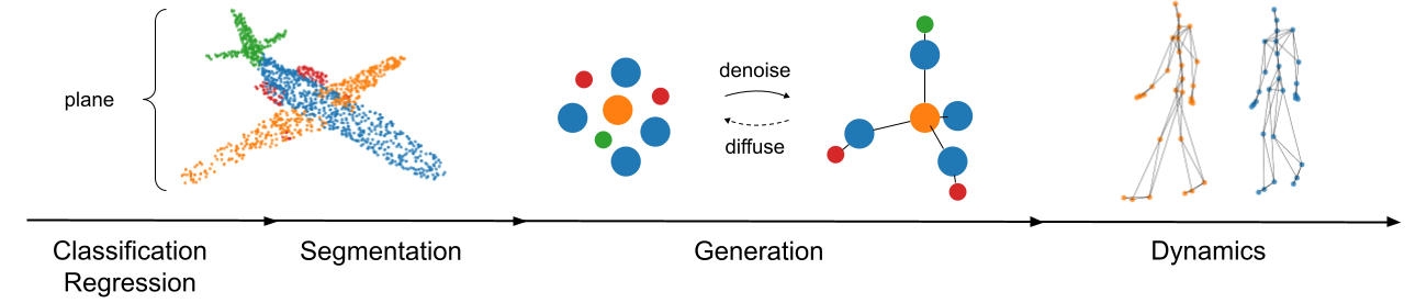
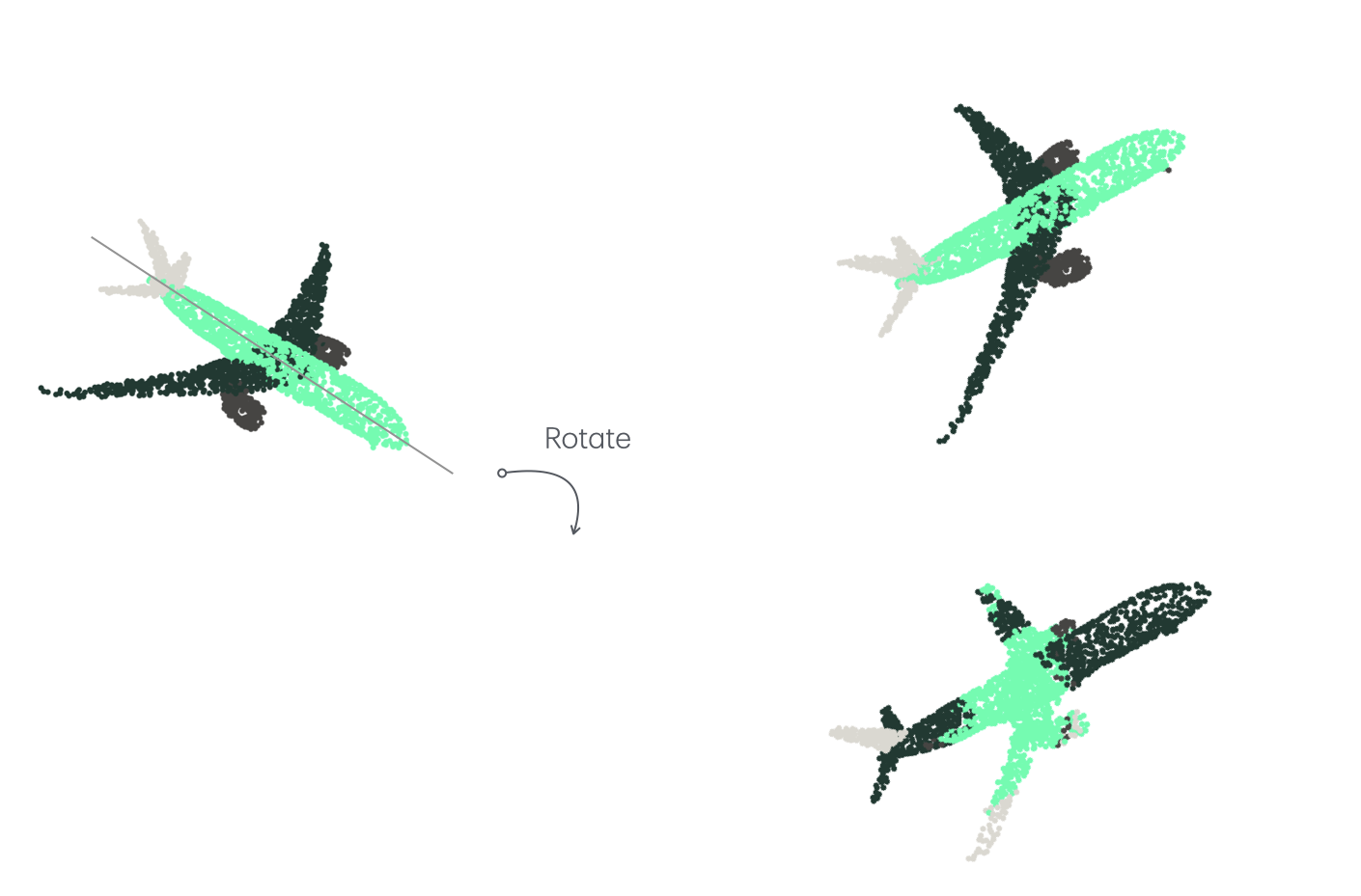
We must also consider task complexity, shown in Figure 1. We will focus the study on tasks that require either invariance or equivariance and formulate the following hypothesis to study the role of equivariance in tasks with varying geometric complexity.
Hypothesis 2 (Geometric complexity)
The advantages of equivariant methods over non-equivariant ones become more pronounced in tasks that require a stricter form of equivariance.
-
(a)
For invariant tasks the gap in performance between equivariant and non-equivariant models will be less pronounced than in equivariant tasks.
-
(b)
There is a hierarchy of tasks in terms of how geometrically demanding they are, and thus to what extent equivariance is needed.
-
•
Low complexity: Invariant tasks like classification and regression;
-
•
Moderate complexity: Equivariant tasks that make point-wise scalar predictions relative to a geometry (shape), like segmentation;
-
•
High complexity: Equivariant tasks that make point-wise vector predictions relative to a geometry, like denoising diffusion models and dynamics forecasting methods.
The performance gap will increase with geometric complexity.
-
•
Next, we want to investigate the effect of expanding the domain over which features are organized. In group convolutions, one typically adds an additional axis to store features that have a meaning relative to a set or grid of reference poses. For example, consider a classical CNN with a 256-dimensional feature vector per node (Table 1: rows 1-4, ). A G-CNN with the same number of independent features per node effectively has dimensional feature vectors per node and arguably more representation capacity (rows 5-11). To test the following hypothesis, models with equal representation capacity need to be compared.
Hypothesis 3 (Representation capacity)
Under the same representation capacity (e.g. same number of total channels per node), equivariant and non-equivariant models perform on par.
The previous hypothesis is likely to be rejected because even when the dimensionality of the representation spaces might be the same (e.g. models 1-4 in comparison to 16-19), the invariant models are constrained to only produce invariant feature vectors and thus have a smaller effective dimensionality. For all models, we have universal approximation results (invariant or equivariant), so as long as we reach the limit of performance per model we cannot say that one model was structurally limited to finding the solution, especially when considering strictly invariant/equivariant tasks. Then, what could cause a difference in performance, if both types of models could represent the optimal solution, in principle? We thus formulate the following two hypotheses.
Hypothesis 4 (Kernel constraint)
We expect that unconstrained (translational) models (Eq. 3) outperform (roto-translation) models (Eq. 4) over as the former is less constrained. Similarly, we expect that equivariant group convolution methods (Eq. 7) outperform the constrained convolutional models (Eq. 4), even when matched in representation capacity.
Considering the above hypothesis, it might also be beneficial to break equivariance, i.e., allow a model to learn non-equivariant solutions even though it is primed for equivariant solutions. In Section 4 we test several options for breaking equivariance by providing features defined in the global coordinate system as input features. Not only will this break equivariance it will also provide the models with an explicit representation of geometry, whereas strictly equivariant models only have access to geometry implicitly via pair-wise relations that condition the convolution kernels. We thus formulate the following.
Hypothesis 5 (Symmetry breaking and explicit geometric representations)
In non-equivariant tasks, where symmetry breaking is allowed, models that are provided with explicit geometric information (such as taking coordinates as features) outperform those that do not have this information.
3.2 Architecture
Based on (Bekkers et al., 2024), we design a model class called Rapidash that is capable of incorporating various forms of equivariances, and thus has the flexibility to test the above hypotheses.
ConvNext blocks
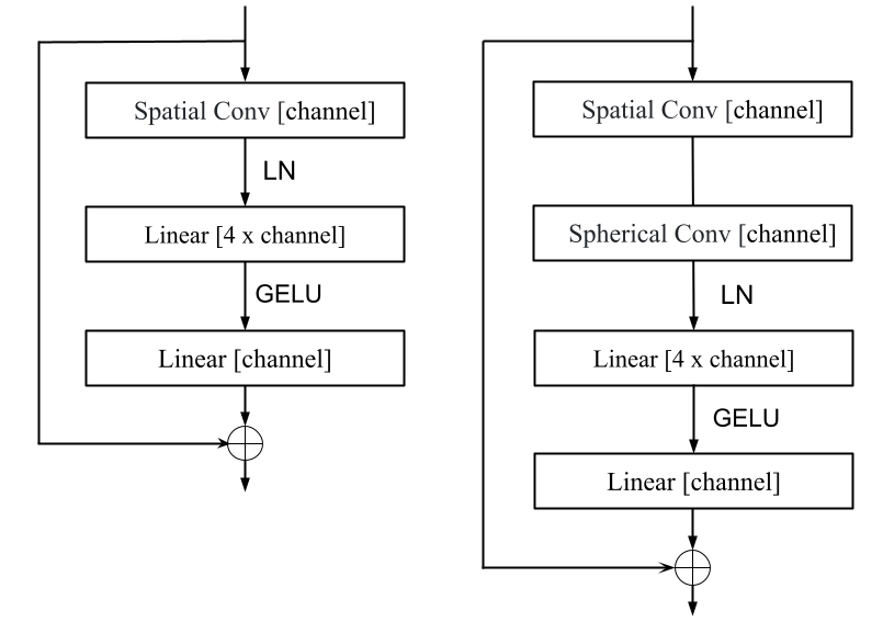
Our architecture is fully convolutional and is based on the ConvNext block from Liu et al. (2022). See 2 for an illustration. The block consists of the following sequence of operations: a depth-wise separable convolution, followed by a LayerNorm, then a point-wise linear layer that increases the channel dimension four-fold, a GELU activation, and a linear back to the original channel dimensions. This output is added via a skip connection. The depth-wise separable convolution is either implemented via Eq. 3 or 4 for the classical (base space ) architecture, and via Eq. 8 and 9 in the case. Thus, the only difference to the point-cloud implementation of ConvNext is that in our group convolutional implementation, the convolution is over instead of just over .
Rapidash
To handle large point clouds, such as in the ShapeNet experiments, we need down- and up-sampling layers. Downsampling happens via strided convolution, by subsampling the point cloud using farthest point sampling, and only evaluating the convolution at the down-sampled points. Up-sampling does the inverse; it is also just a convolution layer, but sampled on a denser grid. See figure 2. The resulting model is in essence a multi-scale version of PNITA (Bekkers et al., 2024) and will be referred to as Rapidash.
4 Experiments
We present a thorough analysis of the hypotheses mentioned in Section 3 through a series of experiments on various point cloud datasets like Shapenet 3D, QM9, and the CMU human motion prediction dataset, which are tasks with increasing levels of complexity (Fig. 1). For each of the experiments, we have different variations of Rapidash arising from equations Eq. 3 or 4 for and Eq. 8 and 9 in case, all with different input variations. For each table, the top section shows models with equivariance, and the bottom section shows models with equivariance. Symmetry breaking is indicated by: ! (), ! ( or ), and ! (conditional ). A ✓indicates an option is used, ✗, indicates it is not used, and "-" indicates the option is not available. ➟ marks the model with maximal equivariance and information access. All experiments use Rapidash under different equivariance constraints. Note, all models have implicit access to positional information via pair-wise geometric attributes. For implementation details see App. A.5. Our code is made available at [see anonymous supplementary .zip file].
4.1 3D point cloud segmentation and generation experiments
In this experiment, we evaluate our models on the ShapeNet 3D dataset (Chang et al., 2015) part segmentation and generation tasks. ShapeNet consists of 16,881 shapes from 16 categories. Each shape is annotated with up to six parts, totaling 50 parts. We use the point sampling of 2,048 points and the train/validation/test split from (Qi et al., 2017). We compare our models to various state-of-the-art methods like PointnXt (Qian et al., 2022), Deltaconv (Wiersma et al., 2022), and GeomGCNN (Srivastava & Sharma, 2021)for the part segmentation task. For the generation task, we compare to the latent diffusion model, LION, (Zeng et al., 2022).
| Rapidash with internal Equivariance Constraint | |||||||||||||||||||||||||||||||||||||||
|
|
|
|
|
|
|
|
|
|
|
|
||||||||||||||||||||||||||||
| 1 | ✗ | - | ✗ | - | - | - | |||||||||||||||||||||||||||||||||
| 2 | ✗ | - | ✓ | - | - | - | |||||||||||||||||||||||||||||||||
| 3 | ✓ | - | ✗ | - | - | none | |||||||||||||||||||||||||||||||||
| 4 | ✓ | - | ✓ | - | - | none | - | ||||||||||||||||||||||||||||||||
| \hdashline5 | ✗ | ✗ | ✗ | ✗ | ✗ | - | |||||||||||||||||||||||||||||||||
| 6 | ✗ | ✗ | ✗ | ✗ | ✓ | ||||||||||||||||||||||||||||||||||
| 7 | ✗ | ✗ | ✗ | ✓ | ✗ | - | |||||||||||||||||||||||||||||||||
| ➟ 8 | ✗ | ✗ | ✗ | ✓ | ✓ | - | |||||||||||||||||||||||||||||||||
| 9 | ✗ | ✓ | ✗ | ✗ | ✗ | - | |||||||||||||||||||||||||||||||||
| 10 | ✗ | ✓ | ✗ | ✗ | ✓ | ||||||||||||||||||||||||||||||||||
| 11 | ✗ | ✓ | ✗ | ✓ | ✗ | - | |||||||||||||||||||||||||||||||||
| 12 | ✗ | ✓ | ✗ | ✓ | ✓ | - | |||||||||||||||||||||||||||||||||
| \hdashline13 | ✗ | ✗ | ✓ | ✗ | ✗ | - | |||||||||||||||||||||||||||||||||
| 14 | ✓ | ✗ | ✗ | ✗ | ✗ | none | |||||||||||||||||||||||||||||||||
| 15 | ✓ | ✗ | ✓ | ✗ | ✗ | none | - | ||||||||||||||||||||||||||||||||
| Rapidash with Internal Equivariance Constraint | |||||||||||||||||||||||||||||||||||||||
| 16 | ✗ | - | ✗ | - | - | ||||||||||||||||||||||||||||||||||
| 17 | ✗ | - | ✓ | - | - | - | |||||||||||||||||||||||||||||||||
| 18 | ✓ | - | ✗ | - | - | none | |||||||||||||||||||||||||||||||||
| 19 | ✓ | - | ✓ | - | - | none | - | ||||||||||||||||||||||||||||||||
| Reference methods from literature | |||||||||||||||||||||||||||||||||||||||
| LION | - | - | - | - | - | - | - | - | - | 51.85 | - | ||||||||||||||||||||||||||||
| PVD | - | - | - | - | - | - | - | - | - | 58.65 | - | ||||||||||||||||||||||||||||
| DPM | - | - | - | - | - | - | - | - | - | 62.30 | - | ||||||||||||||||||||||||||||
| DeltaConv | - | - | - | - | - | - | - | 86.90 | - | - | - | ||||||||||||||||||||||||||||
| PointNeXt | - | - | - | - | - | - | - | 87.00 | - | - | - | ||||||||||||||||||||||||||||
| GeomGCNN333GeomGCNN is trained with 1024 points instead of 2048. | - | - | - | - | - | - | - | 89.10 | - | - | - | ||||||||||||||||||||||||||||
4.2 Molecular property prediction and Molecule generation (discovery)
For predicting molecular properties and generating molecules, we use QM9 (Ramakrishnan R., 2014), a dataset which consists of 130k small molecules and their 3-dimensional coordinates, along with molecular properties, integer-valued atom charges, and atom coordinates. It contains up to 9 heavy atoms and 29 atoms including hydrogens. We use the train/val/test partitions introduced in Gilmer et al. (2017), which consists of 100K/18K/13K samples respectively for each partition. We evaluate the prediction of molecular properties using the MAE metric and compare these with EGNN (Satorras et al., 2021), Dimenet++ (Gasteiger et al., 2022) and SE(3)- Transformer Fuchs et al. (2020)
For the molecule generation (discovery) task, we train an equivariant generative model that uses equivariant denoising layers in a diffusion model like that in Karras et al. (2022) to unconditionally generate molecules. We evaluate molecular generation on metrics from Hoogeboom et al. (2022) like atomic stability and molecule stability. We introduce a new metric, discover, defined as a product of validity unique novelty , which represents a discovery rate for a generated sample. It represents the fraction of generated samples that are jointly valid, unique, and new, which is crucial for discovering new molecules. We compare our models with EGNN-based denoising diffusion (Ho et al., 2020) model like Hoogeboom et al. (2022), , MiDi (Vignac et al., 2023), and PNITA (Bekkers et al., 2024) based diffusion model.
| Rapidash with internal Equivariance Constraint | |||||||||||||||||||||||||||||||||||||||
| Regression | Generation | ||||||||||||||||||||||||||||||||||||||
|
|
|
|
|
|
|
|
|
|
|
|
||||||||||||||||||||||||||||
| 1 | ✗ | - | - | - | - | ||||||||||||||||||||||||||||||||||
| 2 | ✓ | - | none | ||||||||||||||||||||||||||||||||||||
| \hdashline3 | ✗ | ✗ | |||||||||||||||||||||||||||||||||||||
| ➟ 4 | ✗ | ✓ | |||||||||||||||||||||||||||||||||||||
| 5 | ✓ | ✗ | none | ||||||||||||||||||||||||||||||||||||
| Rapidash with Internal Equivariance Constraint | |||||||||||||||||||||||||||||||||||||||
| 6 | ✗ | - | |||||||||||||||||||||||||||||||||||||
| 7 | ✓ | - | none | ||||||||||||||||||||||||||||||||||||
| Reference methods from literature | |||||||||||||||||||||||||||||||||||||||
| EGNN | - | - | - | - | 0.0290 | 0.0710 | 29.00 | 98.7 | 82.0 | - | - | ||||||||||||||||||||||||||||
| DimeNet++∗ | - | - | - | - | 0.0297 | 0.0435 | 24.60 | - | - | - | - | ||||||||||||||||||||||||||||
| -T | - | - | - | - | 0.1420 | 0.0510 | 53.00 | - | - | - | - | ||||||||||||||||||||||||||||
| MiDi (adaptive)∗∗ | - | - | - | - | - | - | - | 99.8 | 97.5 | 64.5 | - | ||||||||||||||||||||||||||||
| Clifford-EDM | - | - | - | - | - | - | - | 99.5 | 93.4 | 89.5 | - | ||||||||||||||||||||||||||||
| EGNN-EDM | - | - | - | - | - | - | - | 99.25 | 90.73 | 89.5 | - | ||||||||||||||||||||||||||||
| PNITA | - | - | - | - | - | - | - | 98.9 | 87.8 | - | - | ||||||||||||||||||||||||||||
| ∗ Not a fair comparison as trained for longer. ∗∗Not a fair comparison, as MiDi uses open Babel optimization procedure. | |||||||||||||||||||||||||||||||||||||||
4.3 Human motion prediction task
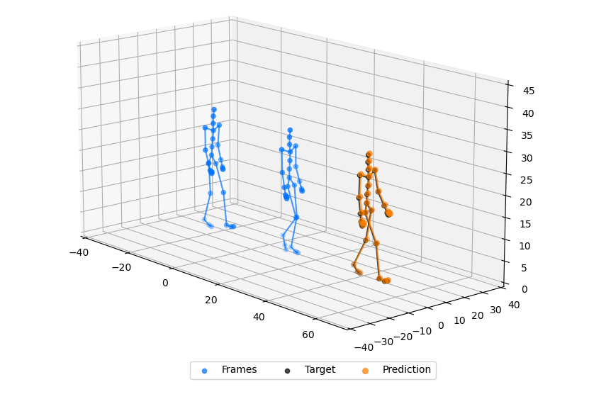
In table 3, we evaluate our models on the CMU Human Motion Capture dataset (Gross & Shi, 2001), consisting of 31 equally connected nodes, each representing a specific position on the human body during walking. Given node positions at a random frame, the objective is to predict node positions after 30 timesteps. As per Huang et al. (2022) we use the data of the 35th human subject for the experiment. We compare our models to NRI (Kipf et al., 2018), EGNN (Satorras et al., 2021), CEGNN (Ruhe et al., 2023) and CSMPN Liu et al. (2024) and show improved performance. We demonstrate that equivariant architectures enable better performance in motion prediction. See Fig:5 in Appendix.
| Rapidash with internal Equivariance Constraint | |||||||||||||||||||||||||||||||||||
|
|
|
|
|
|
|
|
|
|
|
|||||||||||||||||||||||||
| 1 | ✗ | - | ✗ | - | - | ||||||||||||||||||||||||||||||
| 2 | ✗ | - | ✓ | - | - | ||||||||||||||||||||||||||||||
| 3 | ✓ | - | ✗ | - | - | none | |||||||||||||||||||||||||||||
| 4 | ✓ | - | ✓ | - | - | none | |||||||||||||||||||||||||||||
| 5 | ✗ | ✗ | ✗ | ✗ | ✗ | 6.17 | 8.71 | ||||||||||||||||||||||||||||
| 6 | ✗ | ✗ | ✗ | ✓ | ✗ | ||||||||||||||||||||||||||||||
| ➟ 7 | ✗ | ✗ | ✗ | ✓ | ✓ | 4.95 | 6.71 | ||||||||||||||||||||||||||||
| 8 | ✗ | ✓ | ✗ | ✗ | ✗ | 7.26 | 10.03 | ||||||||||||||||||||||||||||
| 9 | ✗ | ✓ | ✗ | ✗ | ✓ | 4.95 | 7.57 | ||||||||||||||||||||||||||||
| 10 | ✗ | ✓ | ✗ | ✓ | ✗ | 5.31 | 7.99 | ||||||||||||||||||||||||||||
| 11 | ✗ | ✓ | ✗ | ✓ | ✓ | 5.14 | 7.50 | ||||||||||||||||||||||||||||
| \hdashline12 | ✗ | ✗ | ✓ | ✗ | ✗ | ||||||||||||||||||||||||||||||
| 13 | ✓ | ✗ | ✗ | ✗ | ✗ | none | 5.29 | 60.82 | |||||||||||||||||||||||||||
| 14 | ✓ | ✗ | ✓ | ✗ | ✗ | none | 5.31 | 65.80 | |||||||||||||||||||||||||||
| Rapidash with Internal Equivariance Constraint | |||||||||||||||||||||||||||||||||||
| 15 | ✗ | - | ✗ | - | - | ||||||||||||||||||||||||||||||
| 16 | ✗ | - | ✓ | - | - | ||||||||||||||||||||||||||||||
| 17 | ✓ | - | ✗ | - | - | none | |||||||||||||||||||||||||||||
| 18 | ✓ | - | ✓ | - | - | none | |||||||||||||||||||||||||||||
| Reference methods from literature | |||||||||||||||||||||||||||||||||||
| TFN | - | - | - | - | - | - | - | 66.90 | - | - | |||||||||||||||||||||||||
| EGNN | - | - | - | - | - | - | - | 31.70 | - | - | |||||||||||||||||||||||||
| CGENN | - | - | - | - | - | - | - | 9.41 | - | - | |||||||||||||||||||||||||
| CSMPN | - | - | - | - | - | - | - | 7.55 | - | - | |||||||||||||||||||||||||
5 Results
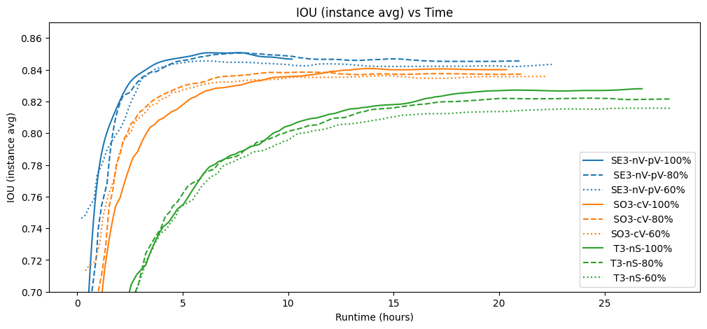
Hypothesis 1 is accepted: Equivariant methods are more data-efficient then their non-equivariant counter part. The hypothesis is tested on Shapenet segmentation for various dataset size regimes as shown in Fig. 3 and Tab. 5 in the Appendix.
Hypothesis 2 is accepted: The advantage of equivariant models gets more pronounced with task complexity. Although, on all experiments the equivariant models have an edge over non-equivariant models, this improvement is more pronounced in complex and equivariant tasks, such as QM9 regression and generation (Tab. 2), Shapenet generation (Tab. 1) and motion prediction (Tab. 3), in which we note that both Shapenet generation and CMU motion prediction do not require equivariance, but are complex geometric tasks.
Hypothesis 3 is rejected: Increasing model capacity by increasing the number of channels does not lead to a performance gain as seen by the group convolutional methods. The performance of low vs high capacity (compared gray vs regular numbers in the tables) is often negligible. The results suggest that all of the models are already maxed-out in net capacity to reach optimal performance.
Hypothesis 4 is accepted: For equivariant tasks, having less constraints on the model is beneficial. See, e.g., Tab. 1, comparing models 1-4 with models 16-19, the latter being less constrained, and performing significantly better. Consider also the QM9 experiments (Tab. 2) which is an equivariant task. All models 1,2 and 5-12 are equivariant and universal approximators and should be able to solve the problem. Models 1-2 however use constrained kernels (symmetric, distance-based) while the group convolutional models are not. The latter largely outperforms the former.
Hypothesis 5 is accepted: Providing explicit geometric information can improve performance, even when breaking symmetry. This is, e.g., observed in the tables by comparing the group convolutional models that take either coordinates as scalars (breaks equivariance) or as vectors (maintains equvariance) against those models that do not take any coordinate information as input.
6 Discussion and Conclusion
Discussion Beyond hypothesis insights, our basic convolutional architecture (Rapidash) performs exceptionally well on all considered tasks, often reaching state-of-the-art (SotA) performance, s.a. on ShapeNet/QM9 generation and CMU motion prediction. Surprisingly, even non-equivariant methods perform well on equivariant tasks, though not at SotA level and without equivariant generalization guarantees. These results support the "convolution is all you need" idea (Cohen et al., 2019; Bekkers et al., 2024), contrasting the popular "attention-is-all-you-need" claim (Vaswani, 2017). The generalizability of the presented hypotheses remains to be tested outside of the class of convolutional architectures, to which Rapidash belongs. Conclusion In this work, we conducted a comprehensive evaluation of equivariant and non-equivariant models across various tasks of varying geometric complexities. In the debate of equivariant vs non-equivariant models, we provide strong evidence in favor of introducing structure over mere scaling. Specifically, we find that equivariant models (1) are more data efficient, (2) increasingly outpace non-equivariant models when increasing task geometric complexity, and (3) see performance benefits from targeted symmetry breaking.
References
- Bekkers (2019) Erik J Bekkers. B-spline cnns on lie groups. In International Conference on Learning Representations, 2019.
- Bekkers et al. (2018) Erik J Bekkers, Maxime W Lafarge, Mitko Veta, Koen AJ Eppenhof, Josien PW Pluim, and Remco Duits. Roto-translation covariant convolutional networks for medical image analysis. In Medical Image Computing and Computer Assisted Intervention–MICCAI 2018: 21st International Conference, Granada, Spain, September 16-20, 2018, Proceedings, Part I, pp. 440–448. Springer, 2018.
- Bekkers et al. (2024) Erik J Bekkers, Sharvaree Vadgama, Rob Hesselink, Putri A Van der Linden, and David W. Romero. Fast, expressive se(n) equivariant networks through weight-sharing in position-orientation space. In The Twelfth International Conference on Learning Representations, 2024. URL https://openreview.net/forum?id=dPHLbUqGbr.
- (4) Johannes Brandstetter, Rob Hesselink, Elise van der Pol, Erik J Bekkers, and Max Welling. Geometric and physical quantities improve e (3) equivariant message passing. In International Conference on Learning Representations.
- Bronstein et al. (2021) Michael M Bronstein, Joan Bruna, Taco Cohen, and Petar Veličković. Geometric deep learning: Grids, groups, graphs, geodesics, and gauges. arXiv preprint arXiv:2104.13478, 2021.
- Chang et al. (2015) Angel X. Chang, Thomas Funkhouser, Leonidas Guibas, Pat Hanrahan, Qixing Huang, Zimo Li, Silvio Savarese, Manolis Savva, Shuran Song, Hao Su, Jianxiong Xiao, Li Yi, and Fisher Yu. Shapenet: An information-rich 3d model repository, 2015. URL https://arxiv.org/abs/1512.03012.
- Chollet (2017) François Chollet. Xception: Deep learning with depthwise separable convolutions. In Proceedings of the IEEE conference on computer vision and pattern recognition, pp. 1251–1258, 2017.
- Cohen & Welling (2016) Taco Cohen and Max Welling. Group equivariant convolutional networks. In International conference on machine learning, pp. 2990–2999. PMLR, 2016.
- Cohen et al. (2019) Taco S Cohen, Mario Geiger, and Maurice Weiler. A general theory of equivariant cnns on homogeneous spaces. Advances in neural information processing systems, 32, 2019.
- Fey & Lenssen (2019) Matthias Fey and Jan Eric Lenssen. Fast graph representation learning with pytorch geometric. arXiv preprint arXiv:1903.02428, 2019.
- Finzi et al. (2020) Marc Finzi, Samuel Stanton, Pavel Izmailov, and Andrew Gordon Wilson. Generalizing convolutional neural networks for equivariance to lie groups on arbitrary continuous data. In Hal Daumé III and Aarti Singh (eds.), Proceedings of the 37th International Conference on Machine Learning, volume 119 of Proceedings of Machine Learning Research, pp. 3165–3176. PMLR, 13–18 Jul 2020. URL https://proceedings.mlr.press/v119/finzi20a.html.
- Finzi et al. (2021) Marc Finzi, Gregory Benton, and Andrew Gordon Wilson. Residual pathway priors for soft equivariance constraints, 2021. URL https://arxiv.org/abs/2112.01388.
- Fuchs et al. (2020) Fabian B. Fuchs, Daniel E. Worrall, Volker Fischer, and Max Welling. Se(3)-transformers: 3d roto-translation equivariant attention networks, 2020. URL https://arxiv.org/abs/2006.10503.
- Gasteiger et al. (2022) Johannes Gasteiger, Shankari Giri, Johannes T. Margraf, and Stephan Günnemann. Fast and uncertainty-aware directional message passing for non-equilibrium molecules, 2022. URL https://arxiv.org/abs/2011.14115.
- Gilmer et al. (2017) Justin Gilmer, Samuel S. Schoenholz, Patrick F. Riley, Oriol Vinyals, and George E. Dahl. Neural message passing for quantum chemistry. In Doina Precup and Yee Whye Teh (eds.), Proceedings of the 34th International Conference on Machine Learning, volume 70 of Proceedings of Machine Learning Research, pp. 1263–1272. PMLR, 06–11 Aug 2017. URL https://proceedings.mlr.press/v70/gilmer17a.html.
- Gross & Shi (2001) Ralph Gross and Jianbo Shi. The cmu motion of body (mobo) database. Technical Report CMU-RI-TR-01-18, Pittsburgh, PA, June 2001.
- Ho et al. (2020) Jonathan Ho, Ajay Jain, and Pieter Abbeel. Denoising diffusion probabilistic models, 2020. URL https://arxiv.org/abs/2006.11239.
- Hoogeboom et al. (2022) Emiel Hoogeboom, Victor Garcia Satorras, Clément Vignac, and Max Welling. Equivariant diffusion for molecule generation in 3d, 2022. URL https://arxiv.org/abs/2203.17003.
- Huang et al. (2022) Wenbing Huang, Jiaqi Han, Yu Rong, Tingyang Xu, Fuchun Sun, and Junzhou Huang. Equivariant graph mechanics networks with constraints, 2022. URL https://arxiv.org/abs/2203.06442.
- Karras et al. (2022) Tero Karras, Miika Aittala, Timo Aila, and Samuli Laine. Elucidating the design space of diffusion-based generative models, 2022. URL https://arxiv.org/abs/2206.00364.
- Kim et al. (2023) Hyunsu Kim, Hyungi Lee, Hongseok Yang, and Juho Lee. Regularizing towards soft equivariance under mixed symmetries. In Andreas Krause, Emma Brunskill, Kyunghyun Cho, Barbara Engelhardt, Sivan Sabato, and Jonathan Scarlett (eds.), Proceedings of the 40th International Conference on Machine Learning, volume 202 of Proceedings of Machine Learning Research, pp. 16712–16727. PMLR, 23–29 Jul 2023. URL https://proceedings.mlr.press/v202/kim23p.html.
- Kingma & Ba (2014) Diederik P Kingma and Jimmy Ba. Adam: A method for stochastic optimization. arXiv preprint arXiv:1412.6980, 2014.
- Kipf et al. (2018) Thomas Kipf, Ethan Fetaya, Kuan-Chieh Wang, Max Welling, and Richard Zemel. Neural relational inference for interacting systems, 2018. URL https://arxiv.org/abs/1802.04687.
- Knigge et al. (2022) David M Knigge, David W Romero, and Erik J Bekkers. Exploiting redundancy: Separable group convolutional networks on lie groups. In International Conference on Machine Learning, pp. 11359–11386. PMLR, 2022.
- Kondor & Trivedi (2018) Risi Kondor and Shubhendu Trivedi. On the generalization of equivariance and convolution in neural networks to the action of compact groups. In International conference on machine learning, pp. 2747–2755. PMLR, 2018.
- Kuipers & Bekkers (2023) Thijs P Kuipers and Erik J Bekkers. Regular se (3) group convolutions for volumetric medical image analysis. In Medical Image Computing and Computer Assisted Intervention–MICCAI 2023. arXiv preprint arXiv:2306.13960, 2023.
- LeCun et al. (2010) Yann LeCun, Koray Kavukcuoglu, and Clément Farabet. Convolutional networks and applications in vision. In Proceedings of 2010 IEEE international symposium on circuits and systems, pp. 253–256. IEEE, 2010.
- Liu et al. (2024) Cong Liu, David Ruhe, Floor Eijkelboom, and Patrick Forré. Clifford group equivariant simplicial message passing networks. In The Twelfth International Conference on Learning Representations, 2024. URL https://openreview.net/forum?id=Zz594UBNOH.
- Liu et al. (2022) Zhuang Liu, Hanzi Mao, Chao-Yuan Wu, Christoph Feichtenhofer, Trevor Darrell, and Saining Xie. A convnet for the 2020s. In Proceedings of the IEEE/CVF conference on computer vision and pattern recognition, pp. 11976–11986, 2022.
- Moskalev et al. (2023) Artem Moskalev, Anna Sepliarskaia, Erik J. Bekkers, and Arnold Smeulders. On genuine invariance learning without weight-tying, 2023. URL https://arxiv.org/abs/2308.03904.
- Paszke et al. (2019) Adam Paszke, Sam Gross, Francisco Massa, Adam Lerer, James Bradbury, Gregory Chanan, Trevor Killeen, Zeming Lin, Natalia Gimelshein, Luca Antiga, et al. Pytorch: An imperative style, high-performance deep learning library. Advances in neural information processing systems, 32, 2019.
- Pertigkiozoglou et al. (2024) Stefanos Pertigkiozoglou, Evangelos Chatzipantazis, Shubhendu Trivedi, and Kostas Daniilidis. Improving equivariant model training via constraint relaxation, 2024. URL https://arxiv.org/abs/2408.13242.
- Petrache & Trivedi (2023) Mircea Petrache and Shubhendu Trivedi. Approximation-generalization trade-offs under (approximate) group equivariance, 2023. URL https://arxiv.org/abs/2305.17592.
- Qi et al. (2017) Charles R. Qi, Hao Su, Kaichun Mo, and Leonidas J. Guibas. Pointnet: Deep learning on point sets for 3d classification and segmentation, 2017. URL https://arxiv.org/abs/1612.00593.
- Qian et al. (2022) Guocheng Qian, Yuchen Li, Houwen Peng, Jinjie Mai, Hasan Abed Al Kader Hammoud, Mohamed Elhoseiny, and Bernard Ghanem. Pointnext: Revisiting pointnet++ with improved training and scaling strategies, 2022. URL https://arxiv.org/abs/2206.04670.
- Ramakrishnan R. (2014) Rupp M.and Von Lilienfeld O.A. Ramakrishnan R., Dral P.O. Quantum chemistry structures and properties of 134 kilo molecules, 2014.
- Ravanbakhsh et al. (2017) Siamak Ravanbakhsh, Jeff Schneider, and Barnabás Póczos. Equivariance through parameter-sharing. In Doina Precup and Yee Whye Teh (eds.), Proceedings of the 34th International Conference on Machine Learning, volume 70 of Proceedings of Machine Learning Research, pp. 2892–2901. PMLR, 06–11 Aug 2017. URL https://proceedings.mlr.press/v70/ravanbakhsh17a.html.
- Ruhe et al. (2023) David Ruhe, Johannes Brandstetter, and Patrick Forré. Clifford group equivariant neural networks, 2023. URL https://arxiv.org/abs/2305.11141.
- Satorras et al. (2021) Vıctor Garcia Satorras, Emiel Hoogeboom, and Max Welling. E (n) equivariant graph neural networks. In International conference on machine learning, pp. 9323–9332. PMLR, 2021.
- Schütt et al. (2023) Kristof T Schütt, Stefaan SP Hessmann, Niklas WA Gebauer, Jonas Lederer, and Michael Gastegger. Schnetpack 2.0: A neural network toolbox for atomistic machine learning. The Journal of Chemical Physics, 158(14), 2023.
- Sosnovik et al. (2019) Ivan Sosnovik, Michał Szmaja, and Arnold Smeulders. Scale-equivariant steerable networks. In International Conference on Learning Representations, 2019.
- Srivastava & Sharma (2021) Siddharth Srivastava and Gaurav Sharma. Exploiting local geometry for feature and graph construction for better 3d point cloud processing with graph neural networks, 2021. URL https://arxiv.org/abs/2103.15226.
- Thomas et al. (2018) Nathaniel Thomas, Tess Smidt, Steven Kearnes, Lusann Yang, Li Li, Kai Kohlhoff, and Patrick Riley. Tensor field networks: Rotation-and translation-equivariant neural networks for 3d point clouds. arXiv preprint arXiv:1802.08219, 2018.
- van der Ouderaa et al. (2022) Tycho F. A. van der Ouderaa, David W. Romero, and Mark van der Wilk. Relaxing equivariance constraints with non-stationary continuous filters, 2022. URL https://arxiv.org/abs/2204.07178.
- Vaswani (2017) A Vaswani. Attention is all you need. Advances in Neural Information Processing Systems, 2017.
- Vignac et al. (2023) Clement Vignac, Nagham Osman, Laura Toni, and Pascal Frossard. Midi: Mixed graph and 3d denoising diffusion for molecule generation, 2023. URL https://arxiv.org/abs/2302.09048.
- Wang et al. (2022) Rui Wang, Robin Walters, and Rose Yu. Approximately equivariant networks for imperfectly symmetric dynamics, 2022. URL https://arxiv.org/abs/2201.11969.
- Weiler & Cesa (2019) Maurice Weiler and Gabriele Cesa. General e (2)-equivariant steerable cnns. Advances in neural information processing systems, 32, 2019.
- Weiler et al. (2018) Maurice Weiler, Fred A Hamprecht, and Martin Storath. Learning steerable filters for rotation equivariant cnns. In Proceedings of the IEEE Conference on Computer Vision and Pattern Recognition, pp. 849–858, 2018.
- Weiler et al. (2021) Maurice Weiler, Patrick Forré, Erik Verlinde, and Max Welling. Coordinate independent convolutional networks–isometry and gauge equivariant convolutions on riemannian manifolds. arXiv preprint arXiv:2106.06020, 2021.
- Wiersma et al. (2022) Ruben Wiersma, Ahmad Nasikun, Elmar Eisemann, and Klaus Hildebrandt. Deltaconv: anisotropic operators for geometric deep learning on point clouds. ACM Transactions on Graphics, 41(4):1–10, July 2022. ISSN 1557-7368. doi: 10.1145/3528223.3530166. URL http://dx.doi.org/10.1145/3528223.3530166.
- Worrall et al. (2017) Daniel E. Worrall, Stephan J. Garbin, Daniyar Turmukhambetov, and Gabriel J. Brostow. Harmonic networks: Deep translation and rotation equivariance. In Proceedings of the IEEE Conference on Computer Vision and Pattern Recognition (CVPR), July 2017.
- Wu et al. (2019) Wenxuan Wu, Zhongang Qi, and Li Fuxin. Pointconv: Deep convolutional networks on 3d point clouds. In Proceedings of the IEEE/CVF Conference on computer vision and pattern recognition, pp. 9621–9630, 2019.
- Zeng et al. (2022) Xiaohui Zeng, Arash Vahdat, Francis Williams, Zan Gojcic, Or Litany, Sanja Fidler, and Karsten Kreis. Lion: Latent point diffusion models for 3d shape generation, 2022. URL https://arxiv.org/abs/2210.06978.
Appendix A Appendix
A.1 Mathematical Prerequisites and Notations
Groups. A group is an algebraic structure defined by a set and a binary operator , known as the group product. This structure must satisfy four axioms: (1) closure, where ; (2) the existence of an identity element such that , (3) the existence of an inverse element, i.e. there exists a such that ; and (4) associativity, where . Going forward, group product between two elements will be denoted as by juxtaposition, i.e., as .
For Special Euclidean group , the group product between two roto-translations and is given by , and its identity element is given by .
Homogeneous Spaces. A group can act on spaces other than itself via a group action , where is the space on which acts. For simplicity, the action of on is denoted as . Such a transformation is called a group action if it is homomorphic to and its group product. That is, it follows the group structure: , and . For example, consider the space of 3D positions , e.g., atomic coordinates, acted upon by the group . A position is roto-translated by the action of an element as .
A group action is termed transitive if every element can be reached from an arbitrary origin through the action of some , i.e., . A space equipped with a transitive action of is called a homogeneous space of . Finally, the orbit of an element under the action of a group represents the set of all possible transformations of by . For homogeneous spaces, for any arbitrary origin .
Quotient spaces. The aforementioned space of 3D positions serves as a homogeneous space of , as every element can be reached by a roto-translation from , i.e., for every there exists a such that . Note that there are several elements in that transport the origin to , as any action with a translation vector suffices regardless of the rotation . This is because any rotation leaves the origin unaltered.
We denote the set of all elements in that leave an origin unaltered the stabilizer subgroup . In subsequent analyses, the symbol is used to denote the stabilizer subgroup of a chosen origin in a homogeneous space, i.e., . We further denote the left coset of in as . In the example of positions we concluded that we can associate a point with many group elements that satisfy . In general, letting be any group element s.t. , then any group element in the left set is also identified with the point . Hence, any can be identified with a left coset and vice versa.
Left cosets then establish an equivalence relation among transformations in . We say that two elements are equivalent, i.e., , if and only if . That is, if they belong to the same coset . The space of left cosets is commonly referred to as the quotient space .
We consider feature maps as multi-channel signals over homogeneous spaces . Here, we treat point clouds as sparse feature maps, e.g., sampled only at atomic positions. In the general continuous setting, we denote the space of feature maps over with . Such feature maps undergo group transformations through regular group representations parameterized by , and which transform functions via .
A.2 Rethinking Equivariant Message Passing as group convolution
Message Passing Consider the graph representation of a point cloud with points in a homogeneous space . Label nodes as and edges between nodes as . Each node has a corresponding coordinate . To each node, a feature is associated, forming a discrete analog to the previously defined dense feature maps , where . Thus, the features associated with a node are . Additionally, one can associate attributes to the edges between nodes as .
Message passing is defined in three steps as follows:
where denotes the set of nodes in the neighborhood of the node.
Group Convolution as Equivariant Message Passing.
Group convolution can be written in terms of the message passing formalism. Given the graph defined above, group convolution can be written as the sum
Defining as the edge feature between a pair of nodes, (1) the message function is , (2) the permutation invariant aggregation function is the sum, and (3) the update map is . Indeed, the message function is a linear map which is determined by the attribute , in this case, determined by the relative pose between two nodes. This dependence on only relative pose underlies both the equivariance and weight sharing of equivariant message passing.
Equivalence Classes and Invariant Attributes. Equivalence classes of position-orientation coordinates with is defined as
where equivalence classes are given by equivalence under group action on each element, i.e.
The list of invariant attributes for position orientation that determine the equivalence relations are given below for completeness (Bekkers et al., 2024).
A.3 Internal vs External Symmetry Breaking
In this section, we provide an analysis of symmetry breaking in equivariant neural networks, distinguishing between what we consider to be two fundamentally different types: external and internal symmetry breaking.
A.3.1 External Symmetry Breaking
External symmetry breaking occurs when an inherently equivariant architecture loses its equivariance properties due to the way inputs are provided to the network. Consider a linear layer designed to be -equivariant for some group (e.g., ). Let be a vector that transforms under the group action, and define as its transformed version in global coordinates. When these coordinates are provided as scalar triplets, they are processed independently with no relation to the group action, thus:
| (10) |
This means the network processes transformed inputs differently, breaking equivariance. In contrast, when inputs are properly specified as vectors that transform under the group action, we maintain equivariance:
| (11) |
Moreover, for truly invariant features (such as one-hot encodings of atom types in QM9), the group action is trivial:
| (12) |
which guarantees invariance of the entire network to group transformations.
A.3.2 Internal Symmetry Breaking
Internal symmetry breaking then refers to the deliberate relaxation of equivariance constraints within the layers themselves. Recent works have explored various approaches to this, including:
-
•
Basis decomposition methods that mix equivariant and non-equivariant components
-
•
Learnable deviation from strict equivariance through regularization
-
•
Progressive relaxation of equivariance constraints during training
In some cases, an internally symmetry-broken layer can be expressed as:
| (13) |
where controls the degree of symmetry breaking, some approaches (e.g., (Wang et al., 2022)) implement schemes where is annealed during training to gradually enforce stricter equivariance.
A.3.3 Combining Internal and External Breaking
In practice, both types of symmetry breaking often occur simultaneously and can interact. For example, a network may use non-stationary filters (internal breaking) while also accepting coordinate inputs in a global reference frame (external breaking). The total degree of symmetry breaking then depends on both mechanisms. Theoretical quantitative bounds on models with task-specific symmetries show that aligning data symmetry with architecture leads to the best model, although having partial or approximate equivariance can improve generalization (Petrache & Trivedi, 2023).
A.3.4 Relationship to Our Work
While our study primarily focuses on external symmetry breaking (cf. the red exclamation marks in our tables), we note that the transition between translation-equivariant layers (Table 1, rows 15-18) and roto-translation equivariant layers (rows 1-4) could be viewed as a form of internal symmetry breaking. However, we distinguish our approach from explicit internal symmetry-breaking methods as we do not implement continuous relaxation of equivariance constraints within layers, but rather compare discrete architectural choices with different symmetry properties.
The experiments demonstrate that carefully controlled symmetry breaking, whether internal or external, can significantly improve model performance when the underlying data exhibits only approximate symmetries. This aligns with recent findings in the field showing the benefits of relaxed equivariance constraints (van der Ouderaa et al., 2022; Kim et al., 2023; Pertigkiozoglou et al., 2024).
A.4 Additional Results and Discussion
Modelnet40C dataset We present Modelnet40 classification results in Tab. 4.
Practical implications of the results Our experiments on ModelNet40 demonstrate similar trends to those discussed in the main paper for the experiments on ShapeNet, QM9 and CMU motion datasets. For a non-equivariant task (low geometric complexity) like classification, we see that equivariant methods perform best, model 6-7 in Tab . 4.
| Rapidash with internal Equivariance Constraint | |||||||||||||||||||||||||||||
|
|
|
|
|
|
|
|
|
|||||||||||||||||||||
| 1 | ✗ | - | ✗ | - | - | ||||||||||||||||||||||||
| 2 | ✗ | - | ✓ | - | - | ||||||||||||||||||||||||
| 3 | ✓ | - | ✗ | - | - | none | |||||||||||||||||||||||
| 4 | ✓ | - | ✓ | - | - | none | |||||||||||||||||||||||
| \hdashline5 | ✗ | ✗ | ✗ | ✗ | ✗ | ||||||||||||||||||||||||
| 6 | ✗ | ✗ | ✗ | ✗ | ✓ | ||||||||||||||||||||||||
| 7 | ✗ | ✗ | ✗ | ✓ | ✗ | ||||||||||||||||||||||||
| 8 | ✗ | ✗ | ✗ | ✓ | ✓ | ||||||||||||||||||||||||
| 9 | ✗ | ✓ | ✗ | ✗ | ✗ | ||||||||||||||||||||||||
| 10 | ✗ | ✓ | ✗ | ✗ | ✓ | ||||||||||||||||||||||||
| 11 | ✗ | ✓ | ✗ | ✓ | ✗ | ||||||||||||||||||||||||
| 12 | ✗ | ✓ | ✗ | ✓ | ✓ | ||||||||||||||||||||||||
| \hdashline13 | ✗ | ✗ | ✓ | ✗ | ✗ | ||||||||||||||||||||||||
| 14 | ✓ | ✗ | ✗ | ✗ | ✗ | none | |||||||||||||||||||||||
| 15 | ✓ | ✗ | ✓ | ✗ | ✗ | none | |||||||||||||||||||||||
| Rapidash with Internal Equivariance Constraint | |||||||||||||||||||||||||||||
| 16 | ✗ | - | ✗ | - | - | ||||||||||||||||||||||||
| 17 | ✗ | - | ✓ | - | - | ||||||||||||||||||||||||
| 18 | ✓ | - | ✗ | - | - | none | |||||||||||||||||||||||
| 19 | ✓ | - | ✓ | - | - | none | |||||||||||||||||||||||
| Reference methods from literature | |||||||||||||||||||||||||||||
| PointNet | - | - | - | - | - | - | - | 90.7 | |||||||||||||||||||||
| PointNet++ | - | - | - | - | - | - | - | 93.0 | |||||||||||||||||||||
| DGCNN | - | - | - | - | - | - | - | 92.6 | |||||||||||||||||||||
Experiments with data reduction in training Experiments in data reduction show that the model variant with the most equivariance, and the most non-symmetry-breaking information (SE3-pV-100%) performed the best, and suffered from the least performance degradation when trained on a smaller percentage of the training set. See Figure 3 for training curves.
| Rapidash with internal Equivariance Constraint | |||||||||||||||||||||||||||||||||||||||
|
|
|
|
|
|
|
|
|
|
|
|
||||||||||||||||||||||||||||
| ➟ 8 | ✗ | ✗ | ✗ | ✓ | ✓ | 85.45 | 85.46 | 85.10 | |||||||||||||||||||||||||||||||
| 9 | ✗ | ✓ | ✗ | ✗ | ✗ | 84.48 | 84.21 | 84.07 | - | ||||||||||||||||||||||||||||||
| Rapidash with Internal Equivariance Constraint | |||||||||||||||||||||||||||||||||||||||
| 17 | ✗ | - | ✓ | - | - | 83.00 | 82.50 | 82.03 | - | ||||||||||||||||||||||||||||||
A.5 Implementation details
We implemented our models using PyTorch (Paszke et al., 2019), utilizing PyTorch-Geometric’s message passing and graph operations modules (Fey & Lenssen, 2019), and employed Weights and Biases for experiment tracking and logging. A pool of GPUs, including A100, A6000, A5000, and 1080Ti, was utilized as computational units. To ensure consistent performance across experiments, computation times were carefully calibrated, maintaining GPU homogeneity throughout.
For all experiments, we use Rapidash with 7 layers with 0 fiber dimensions for and 0 or 8 fiber dimensions for . The polynomial degree was set to 2. We used the Adam optimizer (Kingma & Ba, 2014), with a learning rate of , and with a CosineAnealing learning rate schedule with a warmup period of 20 epochs.
ShapeNet 3D (Generation). For this task, we trained we trained model variation (1-4 & 16-19) in Tab.2 with two different settings of hidden features C = 256 (gray) and C = 2048. The later inflated model was trained to match the representation capacity of the rest of the models. For segmentation task, we use rotated samples and compute IOU with aligned and rotated samples. All the models were trained for 500 epochs with a learning rate and weight decay of .
QM9 (Segmentation and Generation). For the segmentation task, we trained we trained model variation (1,2 & 6,7) in Tab.2 with two different settings of hidden features C = 256 (gray) and C = 2048. The later inflated model was trained to match the representation capacity of the rest of the models. All the models were trained for 500 epochs with a learning rate and weight decay of .
CMU Motion Prediction. For this task we trained model variation (1-4 & 16-19) in Tab.3 with two different settings of hidden features C = 256 (gray) and C = 2048. The later inflated model was trained to match the representation capacity of the models (5-15). All the models were trained for 1000 epochs with a learning rate and weight decay of .
ModelNet40 (Classification) For this task we trained 9 model variations presented in Tab.4 All the models were trained for hidden features C = 256 for 120 epochs with a learning rate and weight decay of .
A.6 Additional figures
Illustrating the effect of equivariant models in ShapeNet segmentation
Human motion prediction using CMU motion capture dataset