Scrambling in charged hairy black holes and the Kasner interior

Abstract

We analyze how the axion parameter, the Einstein-Maxwell-Scalar coupling constant, and charge density from Maxwell field affect the chaotic feature of a charged hairy black hole, as characterized by the quantum Lyapunov exponent. Due to relevant deformation in the boundary theory coming from a scalar bulk field, the bulk solution flows into more general Kasner spacetime in the interior of the black hole, near the singularity. We inject charged shock waves from the asymptotic boundary and calculate the out-of-time-ordered correlators holographically, which can probe chaos. The ratio of the quantum Lyapunov exponent with respect to the surface gravity is reduced as the deformation parameter increased, while the Lyapunov exponent of the deformed geometry can be greater than the axion Reissner-Nordström case when the deformation parameter is large enough. We also study how this deformation, along with the added parameters, affect other chaotic properties such as the butterfly velocity and the scrambling time delay. Furthermore, we also analyze the region where Kasner spacetime undergoes Kasner inversion/transition deeper inside the black hole.

I Introduction

One of the goals of the AdS/CFT correspondence [1] is to reconstruct spacetime geometry in the bulk from the boundary CFT data (see, for example, [2, 3]). Initially, observables at the boundary, such as the expectation value of the boundary field, denoted by $\expectationvalue{\mathcal{O}}$, and the energy-momentum tensor, $\expectationvalue{T_{tt}}$, can reconstruct the spacetime geometry close to the boundary. It is then noticed that the holographic entanglement entropy calculated by the Ryu-Takayanagi entangling surface [4, 5] can penetrate deeper into the bulk region. Furthermore, some entangling surfaces stretch from the left asymptotic boundary to the right one through the entire bulk spacetime and even go into the interior region of a black hole [6]. This surface may shed light on understanding the black hole interior from the boundary perspective.
The entangling surface stretching between the left and right asymptotic boundaries has been used to study the chaotic behavior of a black hole perturbed by the gravitational shock waves [7, 8, 9]. This surface is utilized to calculate mutual information, $I(A;B)$, of two subregions, denoted by $A$ and $B$, that live in the left and right boundary CFT, respectively. The result shows that the black hole amid chaotic behavior with the out-of-time-ordered correlator (OTOC) vanishes in a time scale that is logarithmically dependent on the black hole entropy [10]. The exponential behavior of the vanishing OTOC is controlled by a parameter called the quantum Lyapunov exponent, $\lambda_{L}$, it is analogous to the Lyapunov exponent in a classical chaotic system. The Lyapunov exponent of a black hole is equal to the surface gravity of the black hole and hence saturates the Maldacena-Shenker-Stanford chaos bound [11]. The chaotic behavior of various black holes, including charged and rotating black holes, has been extensively studied using holography in [12, 13, 14, 15, 16, 17, 18, 19, 20]. Chaotic properties of black holes (especially in 2D Jackiw-Teitelboim gravity) can be manifested in the holographic model such as the SYK model [21], which is then gives us hope in simulating traversable wormhole in the lab [22, 23].
The AdS black hole spacetime in the bulk may also contain a scalar field producing the solution of a hairy black hole. In the AdS/CFT dictionary, this scalar field plays an important role in generating deformation in the boundary theory. This deformation creates a holographic renormalization group flow from the UV theory on the boundary to the IR theory near the black hole horizon. If we go deeper into the interior of a black hole, i.e., going into the trans-IR region where the energy scale becomes imaginary, we may arrive in a regime where the geometry becomes Kasner spacetime near the black hole singularity [24, 25, 26, 27]. The quantities in the Kasner spacetime can, in principle, be determined by the boundary data by solving the equations of motion either analytically or numerically. Recently in [28], the Kasner spacetime in the interior has been studied under the influence of some gravitational shock waves which can probe chaos. Recently, holographic complexity [29] and quantum extremal islands [30] are also studied in the Kasner interior of black holes deformed by a scalar hair [31, 32].
In this work, we generalize the study of the chaotic behavior by calculating the Lyapunov exponent $\lambda_{L}$ under the influence of the boundary deformation and its relation to the Kasner geometry in the interior. Aside from the scrambling time studied earlier in [28], the instantaneous Lyapunov exponent of the black hole can also be directly extracted from the mutual information $I(A;B)$ that is calculated holographically [18, 17, 19]. We also generalize the calculation into charged hairy black hole, in which the scalar field interacts with a $U(1)$ gauge field $A_{\mu}$ in the bulk. The interior properties of the charged hairy black hole have been studied as the holographic model of superconductors [24, 26, 27]. Being a black hole model, holographic superconductors may also exhibit chaotic behavior so it is important to study how the interior structure of the holographic superconductor is influenced by the Lyapunov exponent as the boundary data.
The holographic model in [26] also contains the Einstein-Maxwell-Scalar (EMS) coupling term and the axion field. The axion scalar terms was introduced in [33] in the context of holographic superconductors to break translational invariance in the boundary theory. Furthermore, the axion field also presence in the study of holographic phonon [34] which generates finite graviton mass and plays a role in the spontaneous breaking of the translational symmetry as well. On the other hand, the EMS term was introduced in [35] to study the Kasner interior of an asymptotically flat black hole. We study how these parameters: axion parameter, EMS coupling constant, and charge density, influence the chaotic behavior of the black hole in the interior, since these parameters highly influence the interior structure of the black hole [36, 35].
Other than the quantum Lyapunov exponent, we also consider the butterfly velocity of the black hole when it is perturbed by the localized shock waves [9, 13, 20]. We study how this velocity gets affected by the relevant deformation in the boundary and we also study its relation with the Kasner exponent. Although the butterfly velocity only depends on the radius located at the black hole horizon, this chaotic quantity is still related to the OTOC. We expect to find a non-trivial relation between butterfly velocity and the Kasner exponent, and see how the parameters $\zeta,\gamma,\rho$ affect this relation.
Once we inject charged shock waves instead of neutral ones into the black hole, we then expect the shock waves to bounce in the interior region due to interaction between black hole charge and the shock waves charge. This bouncing phenomenon was initially studied in a Reissner-Nordström-AdS black hole background [15] and later extended to charged rotating black hole in the Einstein-Maxwell dilaton-axion theory [19]. Since the bounce happens inside the horizon, it is then important to study its relevance with the emergence of Kasner spacetime. The parameters $\zeta,\gamma,\rho$ might also influence the scrambling time delay, especially its relation with the interior structure of the black hole.
The interior region of the black hole is given by the Kasner spacetime in which $r\phi^{\prime}/\sqrt{2}$ becomes constant, where $\phi(r)$ is a scalar field propagating in the bulk and $r$ is the radial AdS coordinate. In other words, the scalar field diverges logarithmically near the singularity. The aforementioned constant is related to the Kasner exponents, which characterize the spacetime geometry near the singularity. At some radial location inside the horizon, the value of the constant might change, indicating the existence of a second Kasner regime deeper within the interior. This region is called the region after Kasner inversion/transition [26, 27, 37, 38, 28]. We see how the boundary observables, such as the quantum Lyapunov exponent ratios, butterfly velocity, and the scrambling time delay behave after Kasner inversion/transition. We also study how the parameters $\zeta,\gamma,\rho$ affects the boundary observables after Kasner inversion/transition.
The structure of this paper is as follows. In Section 2, we briefly review Kasner geometry in the charged hairy black hole model with EMS coupling and axion field. In Section 3, we calculate mutual information holographically as it is perturbed by charged gravitational shock waves. We extract the instantaneous Lyapunov exponent and study how it is influenced by the presence of boundary deformation. We then study the influence of the $\zeta,\gamma,\rho$ parameters to the Lyapunov exponent as it is deformed by the boundary deformation. The relationship between the Lyapunov and Kasner exponents, as well as how these parameters influence them, are also adressed. Furthermore, we study the impacts of the given parameters on butterfly velocity when the black hole is perturbed by localized shock waves, as well as shock wave bounce in the interior resulting from charge interaction between the black hole and shock waves. In Section 4, we consider another Kasner regime that lies deeper in the interior and analyze how it differs compared to the first Kasner regime when the parameters $\zeta,\gamma,\rho$ are turned on. Finally, we summarize our results and presents some discussions in Section 5.

II Interior of Charged Hairy Black Hole

We use the charged hairy black hole model containing the massive Klein-Gordon field $\phi$, the Maxwell field $A_{\mu}$, and the massless axion field $\Omega$, along with the Einstein-Maxwell-scalar coupling term, which directly couples $F_{\mu\nu}F^{\mu\nu}$, where $F_{\mu\nu}=\partial_{\mu}A_{\nu}-\partial_{\nu}A_{\mu}$, with the scalar field $\phi$. This model is previously studied by [26] to investigate Kasner spacetime in the interior of holographic superconductors. The total action of the four-dimensional model is given by $S=S_{1}+S_{2}+S_{3}$, with action:

$$S_{1} =\int d^{4}x\sqrt{|g|}\quantity(R+\frac{6}{L^{2}}),$$ (1)

$$S_{2} =\int d^{4}x\sqrt{|g|}\bigg{(}-\frac{L^{2}}{4}F_{\mu\nu}F^{\mu\nu}-g^{\mu\nu}\quantity(\partial_{\mu}\phi-iqA_{\mu}\phi)(\partial_{\nu}\phi^{*}+iqA_{\nu}\phi^{*})-\frac{1}{2}m^{2}|\phi|^{2}\bigg{)},$$ (2)

$$S_{3} =\int d^{4}x\sqrt{|g|}\quantity(-\frac{L^{2}}{4}\gamma F_{\mu\nu}F^{\mu\nu}|\phi|^{2}-\frac{1}{L^{2}}K(X)),$$ (3)

where $L$ is the AdS radius, $q$ is the coupling constant of $A_{\mu}$ and $\phi$, and $\gamma$ is the EMS coupling constant. We also introduce the K-essence $K(X)$ with

$$X=\frac{L^{2}}{2}=\sum_{I}g^{\mu\nu}\partial_{\mu}\Omega^{I}\partial_{\nu}\Omega^{I}.$$ (4)

Following [26], the axion field is defined as

$$\Omega^{I}=\zeta x^{I},$$ (5)

with $I=(x,y)$ for some axion parameter $\zeta$. In this case, $X=\zeta^{2}r^{2}$ and the polynomial form of the K-essence is then given by

$$K(X)=X^{n}=(\zeta^{2}r^{2})^{n}.$$ (6)

In the numerical calculations, we mainly focus on $n=1$ case.
We work with a gauge in which the scalar field is real and we assume that it only depends on $r$,

$$\phi=\phi^{*}=\phi(r).$$ (7)

We also choose the Maxwell field to only describes radially-dependence electric potential,

$$A_{\mu}dx^{\mu}=A_{t}dt=\Phi(r)dt.$$ (8)

Both $\phi(r)$ and $\Phi(r)$ create the charged, asymptotically AdS hairy black hole with metric given by the following ansatz,

$$ds^{2}=\frac{L^{2}}{r^{2}}\quantity(-f(r)e^{-\chi(r)}dt^{2}+\frac{dr^{2}}{f(r)}+dx^{2}+dy^{2}).$$ (9)

In this metric, $r$ is the AdS radius coordinate, with $r\rightarrow 0$ corresponding to the AdS boundary, where the CFT lives, and $r\rightarrow\infty$ signifying the black hole singularity in the interior.
The equations of motion are now consist of the Klein-Gordon equation, the Maxwell equation, and the $tt$ and $rr$ component of the Einstein equations which are respectively given by

$$\phi^{\prime\prime}+\phi^{\prime}\quantity(-\frac{2}{r}+\frac{f^{\prime}}{f}-\frac{\chi^{\prime}}{2})+\phi\quantity(-\frac{L^{2}m^{2}}{r^{2}f}+\frac{q^{2}e^{\chi}\Phi^{2}}{f^{2}}+\frac{\gamma r^{2}e^{\chi}\Phi^{\prime 2}}{2f}) =0,$$ (10)

$$\Phi^{\prime\prime}+\Phi^{\prime}\frac{\quantity((\gamma\phi^{2}+1)\chi^{\prime}+4\phi\phi^{\prime})}{(1+\gamma\phi^{2})}-\Phi\frac{2q^{2}\phi^{2}}{r^{2}f(1+\gamma\phi^{2})} =0,$$ (11)

$$\frac{q^{2}e^{\chi}\Phi^{2}\phi^{2}}{f^{2}}-\frac{\chi^{\prime}}{r}+\phi^{\prime 2} =0,$$ (12)

$$\frac{6}{r^{2}}-\frac{6}{r^{2}f}-\frac{2f^{\prime}}{rf}+\frac{L^{2}m^{2}\phi^{2}}{r^{2}f}+\frac{K(X)}{r^{2}f}+\frac{q^{2}e^{\chi}\phi^{2}\Phi^{2}}{f^{2}}+\frac{r^{2}e^{\chi}(\gamma\phi^{2}+1)}{2f}(\Phi^{\prime})^{2}+\phi^{\prime 2} =0.$$ (13)

These equations are coupled and highly non-linear. Therefore, we seek for numerical calculations for solving the equations of motion. We also set the AdS radius to $L=1$ and the horizon radius to $r_{h}=1$ trough the calculations.
With vanishing scalar field $\phi$, the solution is the axion-Reissner-Nordström (aRN) black hole, with

$$f(r) =1-\frac{r^{3}}{r_{h}^{3}}-\frac{r^{2}\zeta^{2}}{2}+\frac{r^{3}\zeta^{2}}{2r_{h}}+\frac{r^{4}\rho^{2}}{4}-\frac{r^{3}r_{h}\rho^{2}}{4},$$ (14)

$$\chi =\text{constant},$$ (15)

$$\Phi(r) =\mu+\rho r.$$ (16)

There are two roots of $f(r)=0$, which gives us the black hole horizon radius $r_{h}$ and the axion-Reissner-Nodrström horizon $r_{\text{aRN}}$.

II.1 Boundary Conditions from the CFT

The equations of motion are second order in both $\phi(r)$ and $\Phi(r)$ and hence we need two boundary conditions for those fields. However, they are first order in $f(r)$ and $\chi(r)$ and thus only one boundary condition for each fields are needed. We integrate the equation of motions numerically from $r_{h}-\delta$ to the boundary at $r=0$ and from $r_{h}+\delta$ to the interior at $r\gg 1$, where $\delta$ is a small number. Therefore, we need to specify proper boundary conditions at the horizon for all fields. Since $f(r)$ is the blackening factor for the black hole solution, we have $f(r_{h})=0$ as the boundary condition. The electric potential needs to vanish at the horizon as well so that the norm of $A_{\mu}$ field is finite there.
Other horizon quantities can be determined by expanding the fields near $r_{h}$,

$$\phi =\phi_{h1}+\phi_{h2}(r-r_{+})+\phi_{h3}(r-r_{+})^{3}+...\;,$$ (17)

$$f =f_{h1}(r-r_{h})+f_{h2}(r-r_{h})^{2}+...\;,$$ (18)

$$\chi =\chi_{h1}+\chi_{h2}(r-r_{h})+\chi_{h3}(r-r_{h})^{2}+...\;,$$ (19)

$$\Phi =\Phi_{h1}(r-r_{h})+\Phi_{h2}(r-r_{h})^{2}+\Phi_{h3}(r-r_{h})^{3}+...\;.$$ (20)

Plugging these expressions to the equations of motion and set the coefficient of the divergent ($\mathcal{O}(1/(r-r_{h})$) parts to zero, we will see that only three quantities are independent. In the numerical calculations, we choose $\phi_{h1},\Phi_{h1},\chi_{h1}$ to be the independent quantities for the boundary conditions at the horizon, while $\phi_{h2}$ and $f_{h1}$ can be determined from there. An explicit calculation gives us

$$f_{h1}=\frac{2m^{2}\phi_{h1}^{2}+2\left(\zeta^{2}r_{h}^{2}\right)^{n}+\gamma r_{h}^{4}e^{\chi_{h1}}\phi_{h1}^{2}\Phi_{h1}^{2}+r_{h}^{4}e^{\chi_{h1}}\Phi_{h1}^{2}-12}{4r_{h}},$$ (21)

and

$$\phi_{h2}=\frac{1}{2} \bigg{(}\frac{2m^{2}\sqrt{4f_{h1}r_{h}-2\left(\zeta^{2}r_{h}^{2}\right)^{n}-r_{h}^{4}e^{\chi_{h1}}\Phi_{h1}^{2}+12}}{f_{h1}r_{h}^{2}\sqrt{2m^{2}+\gamma r_{h}^{4}e^{\chi_{h1}}\Phi_{h1}^{2}}}$$ (22)

$$-\frac{\gamma r_{h}^{2}e^{\chi_{h1}}\Phi_{h1}^{2}\sqrt{4f_{h1}r_{h}-2\left(\zeta^{2}r_{h}^{2}\right)^{n}-r_{h}^{4}e^{\chi_{h1}}\Phi_{h1}^{2}+12}}{f_{h1}\sqrt{2m^{2}+\gamma r_{h}^{4}e^{\chi_{h1}}\Phi_{h1}^{2}}}\bigg{)}.$$

The value of $\phi_{h2}$ is then used as the initial value for the derivative of the field $\phi(r)$, while $f_{h1}$ is then used to calculate the black hole temperature.
Although we need to specify the boundary condition at the horizon for numerical purposes, we need to fix the value of the fields in the asymptotic boundary, where the CFT lives. The solutions of the field equations near the boundary $r\rightarrow 0$ are given by

$$\phi =\phi_{(1)}r+\phi_{(2)}r^{2}+...\;,$$ (23)

$$f =1+f_{(1)}r^{2}+f_{(2)}r^{3}+...+\tilde{f}r^{2n}+...\;,$$ (24)

$$\chi =\chi_{(1)}+\frac{1}{2}\phi_{(2)}^{2}r^{2}+\frac{4}{3}\phi_{(1)}\phi_{(2)}r^{3}+...\;,$$ (25)

$$\Phi =\Phi_{(1)}+\Phi_{(2)}r+q^{2}\phi_{(1)}^{2}\Phi_{(1)}r^{2}+...\;.$$ (26)

These expansion coefficients determine the boundary data from the CFT theory. For example, in the standard quantization scheme, $\phi_{(1)}\equiv\phi_{0}$ is the boundary deformation which plays the role as a source to the boundary scalar field $\mathcal{O}$ that lives in the dual CFT theory. On the other hand, $\phi_{(2)}$ is the expectation value $\expectationvalue{\mathcal{O}}$ as the response of this deformation. Note that we choose $m^{2}=-2/L^{2}$, which satisfies the Breitenlohner-Freedman bound and generates relevant deformation in the CFT. For the Maxwell field, $\Phi_{(1)}\equiv\mu$ determines the chemical potential while $\Phi_{(2)}\equiv-\rho$ determines the charge density of the theory. This charge density will play an important role in making the black hole solution a charged hairy black hole, which reduces to the axion-Reissner-Nordström (aRN) solution when the scalar field $\phi$ is absent.
Since the boundary data $\phi_{(1)}$ and $\Phi_{(2)}$ are fixed, we use shooting method to find suitable values of $\phi_{h1}$ and $\Phi_{h1}$ that gives us correct results at the boundary, i.e., we find the correct value $\phi_{h1}$ and $\Phi_{h1}$ that gives us

$$\lim_{r\rightarrow 0}\frac{\phi(r)}{r}=\phi_{0},$$ (27)

and

$$\lim_{r\rightarrow 0}\Phi^{\prime}(r)=-\rho.$$ (28)

Another boundary data that is also important is $\chi_{(1)}$. For an asymptotically AdS spacetime, we need this value to approach zero in the boundary. To achieve this, we can choose $\chi_{h1}$ and rescale the fields as

$$e^{\chi}\rightarrow a_{1}^{2}e^{\chi},\;\;\;t\rightarrow a_{1}t,\;\;\;\Phi\rightarrow\frac{\Phi}{a_{1}},$$ (29)

so that we have $\chi(0)=0$, by choosing $a_{1}=e^{-\chi(r_{h})/2}$. This scaling does not change the equations of motion and we call this the time scaling symmetry, which sets the black hole temperature to

$$T_{BH}=\frac{\absolutevalue{f_{h1}}e^{-\chi(r_{h})/2}}{4\pi}.$$ (30)

II.2 Flow Through General Kasner Interior

The scalar field $\phi(r)$ propagates through the AdS bulk spacetime and generates relevant deformation $\phi_{0}$ in the boundary CFT theory such that the action of the boundary theory is deformed as

$$\delta S=\int d^{3}x\phi_{0}\mathcal{O},$$ (31)

where $\mathcal{O}$ is the scalar field in the dual theory. This deformation generates a holographic RG flow from the UV theory in the boundary through the IR theory in the bulk (near the horizon). We can also penetrates through the interior of the black hole, where the theory becomes trans-IR. In this regime, the energy scale becomes imaginary and the radial coordinate becomes timelike.
As we go through the interior and approach the singularity, where $r\gg 1$, the fields will behave as

$$\phi =\sqrt{2}c\log r+...\;,$$ (32)

$$f =-f_{K1}r^{3+c^{2}}+...\;,$$ (33)

$$\chi =2c^{2}\log r+\chi_{K1}+...\;,$$ (34)

$$\Phi =\Phi_{K1}r^{1-c^{2}}+\Phi_{K1}+...\;.$$ (35)

With these expansions, and the radial coordinate reparameterization $r=\tau^{-2/(3+c^{2})}$, the metric in the deep interior becomes Kasner spacetime, which can be written as

$$ds^{2}=-d\tau^{2}+a_{t}\tau^{2p_{t}}dt^{2}+a_{x}\tau^{2p_{x}}(dx^{2}+dy^{2}),$$ (36)

and

$$\phi\sim-p_{\phi}\log\tau+\phi_{\tau},$$ (37)

where $a_{t},a_{x},\phi_{\tau}$ are constants. The exponents $p_{t}$ and $p_{x}$ are the Kasner exponents, which along with $p_{\phi}$, are given by

$$p_{x}=\frac{2}{3+c^{2}},\;\;\;p_{t}=\frac{c^{2}-1}{3+c^{2}},\;\;\;p_{\phi}=\frac{2\sqrt{2}c}{3+c^{2}}.$$ (38)

All of the Kasner exponents only depends on the integration constant $c$ near the singularity. This integration constant can be obtained from the boundary conditions in the UV boundary $r\rightarrow 0$ using numerical calculations. After we obtain the fields numerically, $c$ can be extracted from $\frac{r}{\sqrt{2}}\frac{d\phi}{dr}$ at large enough $r$. Therefore, if we find that $rd\phi/dr$ approaches constant for some large value of $r$, we can say that, in this region, we approach the Kasner solution.
One need to notice that the expansion near the singularity in eqs. (32)-(35) come from the case where $\gamma$ and $\zeta$ approaches zero. Therefore, we cannot be sure whether our solution approaches Kasner spacetime for some finite values of $\gamma$ and $\zeta$. In this case, we may check the interior solution numerically by varying $\gamma$ and $\zeta$, and see whether $rd\phi/dr$ approaches constant at some value of $r\gg 1$. This can be seen in Figure 1. One can see that, up to $r=100$, the value of $rd\phi/dr$ approaches constant in the interior, which signal us that we have emergence of Kasner spacetime, although we slightly vary the value of $\gamma$. If we zoom in our result, $rd\phi/dr$ actually oscillates, and the amplitude of the oscillation grows as we go deeper. However, this oscillation is in the order of $\sim 10^{-5}$ and can be neglected. We may also worry about the emergence of different Kasner regime if we go even deeper through the interior. This could happen, as shown in [27]. Nevertheless, it is sufficient for our purposes to consider only the first Kasner regime, where it emerges at the scale of $r$ from 10 to 100. Variation of the $\zeta$ parameter gives us similar conclusions, which can be seen in Figure 2. We will analyze other Kasner universes in future works.

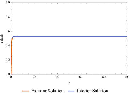
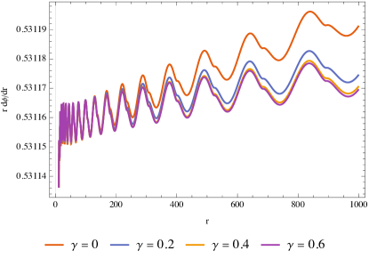
Figure 1: Left: numerical plot of $rd\phi/dr$ both in the exterior with $r\in[0,1]$ and in the interior with $r\in[1,100]$. Right: the zoomed-in version of the interior solution with $r\in[1,1000]$. We vary the value of $\gamma$ from 0 to 0.6 in both cases.

Figure 2: Left: numerical plot of $rd\phi/dr$ both in the exterior with $r\in[0,1]$ and in the interior with $r\in[1,100]$. Right: the interior solution with $r\in[1,1000]$. We vary the value of $\zeta$ from 0 to 0.9 in both cases.

III Mutual Information and Lyapunov Exponent

In this section, we investigate chaotic behavior of the charged hairy black hole using holographic calculations. We calculate the OTOC in the scrambling regime by calculating the mutual information $I(A;B)=S_{A}+S_{B}-S_{A\cup B}$ using holographic entanglement entropy [4, 5]. The calculation of the entanglement entropy $S_{A\cup B}$ involves the calculation of the entangling RT/HRT surfaces which stretch from left to right asymptotic boundaries [6]. This surfaces penetrates through the interior of the black hole. We calculate the area of this surface in a background that is perturbed by charged gravitational shock waves [15, 19] with shock wave parameter given by

$$\alpha=\frac{\beta E_{0}}{S}(1-\Phi_{h}\mathcal{Q})e^{\frac{2\pi t_{w}}{\beta}},$$ (39)

where $\Phi_{h}$ is the black hole’s electric potential and $\mathcal{Q}$ is the shockwaves’ charge per unit energy. Here, $t_{w}$ is the time when the perturbation with energy $E_{0}$ is sent from the left boundary. We use the now-standard method for calculating the entangling surface in the presence of gravitational shock waves.
The mutual information $I(A;B)$ is bounded below by the correlation function $\expectationvalue{\mathcal{O}_{A}\mathcal{O}_{B}}_{w}$ [39], where the state is perturbed at $t_{w}$. The operators $\mathcal{O}_{A}$ and $\mathcal{O}_{B}$ are local operators that act in the subregion $A$ in the left boundary and the subregion $B$ in the right boundary, respectively. The CFT boundary state that is considered here is the entangled thermofield double state $|TFD\rangle$ that represent charged hairy black hole in the AdS dual. We expect that the mutual information of this TFD state will exponentially approaches zero in the scrambling regime, which indicates chaotic behavior of the charged hairy black hole.
It is interesting to study the behavior of the black hole interior from some boundary data that can be determined by $I(A;B)$. This is because the entangling surface of $S_{A\cup B}$ slightly penetrates through the horizon at late times, as we can see later on. Some quantities that can be extracted from this entangling surface is the scrambling time, i.e. the time when $I(A;B)\rightarrow 0$ in the scrambling regime, and the Lyapunov exponent $\lambda_{L}$ that characterizes the chaotic behavior of the black hole. In this work, we focus on the calculation of the Lyapunov exponent. We expect that $\lambda_{L}$ can give us more insight in studying the interior of this charged hairy black hole by studying the relation between $\lambda_{L}$ and the Kasner exponent $p_{t}$. The Lyapunov exponent plays a role in the boundary theory while the Kasner exponent $p_{t}$ determines the interior solution.

III.1 Holographic Calculation of Mutual Information

The entangling surface for $S_{A\cup B}$ can be calculated from the area functional that stretch from the boundary to the turning point $r_{t}>r_{h}$ inside the horizon

$$\mathcal{A}=L_{y}\int_{0}^{r_{t}}\frac{dr}{r^{2}}\quantity(-fe^{-\chi}t^{\prime 2}+\frac{1}{f})^{1/2},$$ (40)

where $r_{t}$ is the turning point that satisfy $\dot{r}=0$, with dot denotes a derivative with respect to $t$ and prime ^′ denotes a derivative with respect to $r$. This area functional is minimized so that the integrand satisfies Euler-Lagrange equation. Since the metric does not depends explicitly on time, there is a conserved quantity $K$ that satisfy

$$K=\frac{-fe^{-\chi}}{r^{2}(-fe^{-\chi}+\dot{r}^{2}/f^{2})^{1/2}}=\frac{(-f(r_{t})e^{-\chi(r_{t})})^{1/2}}{r_{t}^{2}}.$$ (41)

The constant $K$ is chosen at the turning point $r_{t}$ where $\dot{r}=0$.
The relation between boundary time coordinate and the turning point $r_{t}$ can be obtained by integrating the time coordinate in Eq. (41) from the boundary to the turning point,

$$t(r)=t_{b}+\int_{0}^{r}\frac{e^{\chi/2}dr}{r^{2}}\frac{1}{\sqrt{K^{-2}fe^{-\chi}/r^{4}+1}}.$$ (42)

By substituting the expression of $t^{\prime}$ in (42) into the area functional, we get

$$\mathcal{A}=L_{y}\int_{0}^{r_{t}}\frac{dr}{r^{2}\sqrt{f}}\frac{1}{\sqrt{K^{2}r^{4}/fe^{-\chi}+1}}.$$ (43)

We integrate this area functional from the boundary located at $r=0$ to the turning point inside the horizon $r_{t}$. The total area that gives the entropy $S_{A\cup B}$ is four times this area.
When integrating the area functional, we seperate the integration into three segments, following [12, 18, 19]. The first segment is integration from the boundary with $(U,V)=(1,-1)$ to the horizon with $(U,V)=(U_{1},0)$. The second segment stretches from the horizon with $(U,V)=(U_{1},0)$ to the turning point at $r=r_{t}$ denoted by $(U,V)=(U_{2},V_{2})$. The third segment now runs from the turning point at $(U,V)=(U_{2},V_{2})$ to the the location deformed by the shock waves $\alpha$ at the horizon with $(U,V)=(0,\alpha/2)$. In this case, $U,V$ are the Kruskal coordinates.
The first segment gives us

$$U_{1}^{2}=\exp\quantity[\frac{4\pi}{\beta}\int_{0}^{r_{h}}\frac{e^{\chi/2}dr}{f}\quantity(1-\frac{1}{\sqrt{K^{-2}fe^{-\chi}/r^{4}+1}})],$$ (44)

the second segment gives us

$$U_{2}^{2}=\exp\quantity[\frac{4\pi}{\beta}\int_{0}^{r_{t}}\frac{e^{\chi/2}dr}{f}\quantity(1-\frac{1}{\sqrt{K^{-2}fe^{-\chi}/r^{4}+1}})],$$ (45)

and

$$V_{2}=\frac{1}{U_{2}}\exp\quantity[\frac{4\pi}{\beta}\int_{\bar{r}}^{r_{t}}\frac{e^{\chi/2}dr}{f}],$$ (46)

while the final segment provides us with the relation between $\alpha$ and the preceding integrals,

$$\frac{\alpha^{2}}{4V_{2}^{2}}=\exp\quantity[\frac{4\pi}{\beta}\int_{r_{t}}^{r_{h}}\frac{e^{\chi/2}dr}{f}\quantity(1-\frac{1}{\sqrt{K^{-2}fe^{-\chi}/r^{4}+1}})]=\frac{U_{1}^{2}}{U_{2}^{2}}.$$ (47)

The radial location $\bar{r}$ that appears in eq. (46) is defined such that the value of $r_{*}$ at this point is zero inside the horizon. The final integral in eq. (47) gives us the the shock wave parameter

$$\alpha=2\exp\quantity(Q_{1}+Q_{2}+Q_{3}),$$ (48)

where

$$Q_{1} =\frac{4\pi}{\beta}\int_{\bar{r}}^{r_{t}}\frac{e^{\chi/2}dr}{f},$$ (49)

$$Q_{2} =-\frac{2\pi}{\beta}\int_{0}^{r_{h}}\frac{e^{\chi/2}dr}{f}\quantity(1-\frac{1}{\sqrt{K^{-2}fe^{-\chi}/r^{4}+1}}),$$ (50)

$$Q_{3} =-\frac{4\pi}{\beta}\int_{r_{h}}^{r_{t}}\frac{e^{\chi/2}dr}{-f}\quantity(\frac{1}{\sqrt{K^{-2}fe^{-\chi}/r^{4}+1}}-1).$$ (51)

In contrast with the value of the shock waves parameters found in previous works [12, 16, 18, 19], we find that in this case, $\alpha$ depends on the function $\chi$ and thus it is also controlled by the boundary deformation $\phi_{0}$. Furthermore, the functions $f(r)$ and $\chi(r)$ are also controlled by other parameters in this charged hairy black hole such as the gauge field coupling constant $q$, axion field strength $\lambda$, and the EMS coupling parameter $\gamma$.
We are interested in the limit where $\alpha\rightarrow\infty$. This limit can be achieved by setting the boundary time such that the turning point approach some value $r_{t}\rightarrow r_{c}$, where $r_{c}$ satisfies

$$\frac{d}{dr}\quantity(\frac{fe^{-\chi}}{r^{4}})\bigg{|}_{r=r_{c}}=0.$$ (52)

In this limit, both $Q_{1}$ and $Q_{2}$ integrals remain finite while $Q_{3}$ logarithmically diverge as $r_{t}\rightarrow r_{c}$. The value of the critical radius $r_{c}$ can be obtained numerically. As $r_{t}\rightarrow r_{c}$, the main contribution of the area functional in eq. (43) comes from the region near $r_{c}$. Therefore, the area is linearly proportional to $Q_{3}$, and hence depends on $\alpha$ logarithmically,

$$\mathcal{A}\approx L_{y}\quantity(\frac{\beta}{4\pi})\quantity[\frac{-f(r_{c})e^{-\chi(r_{c})}}{r_{c}^{4}}]^{1/2}Q_{3}\approx L_{y}\quantity(\frac{\beta}{4\pi})\quantity[\frac{-f(r_{c})e^{-\chi(r_{c})}}{r_{c}^{4}}]^{1/2}\log\alpha.$$ (53)

From the result of the gravitational shock waves parameter $\alpha$, one can see that this area functional grows linearly in the insertion time $t_{w}$.
The entanglement entropy $S_{A\cup B}$ is proportional to the area $\mathcal{A}_{A\cup B}$ that is given by four times the area of a minimal surface $\mathcal{A}$ divided by $4G_{N}$. Therefore, the mutual information $I(A;B)$ is given by

$$I(A;B) =S_{A}+S_{B}-S_{A\cup B}$$ (54)

$$=\frac{\mathcal{A}_{A}+\mathcal{A}_{B}}{4G_{N}}-\frac{L_{y}}{2G_{N}}\quantity[\frac{-f(r_{c})e^{-\chi(r_{c})}}{r_{c}^{4}}]^{1/2}t_{w}+\frac{L_{y}}{G_{N}}\quantity(\frac{\beta}{4\pi})\quantity[\frac{-f(r_{c})e^{-\chi(r_{c})}}{r_{c}^{4}}]^{1/2}\log S$$ (55)

$$\;\;\;\;\;\;\;\;+\frac{L_{y}}{G_{N}}\quantity(\frac{\beta}{4\pi})\quantity[\frac{-f(r_{c})e^{-\chi(r_{c})}}{r_{c}^{4}}]^{1/2}\log\frac{1}{1-\Phi_{h}\mathcal{Q}},$$

where $\mathcal{A}_{A}$ and $\mathcal{A}_{B}$ are the Ryu-Takayanagi surfaces correspond to the subregions $A$ and $B$. In calculating this mutual information, we take the energy of the shock waves $E$ to be at the order of a few Hawking quanta so that $\beta E\sim 1$. The mutual information is real-valued since $f(r_{c})$ is negative when the critical radius $r_{c}$ lies inside the horizon. Furthermore, it is also positive-valued since when $\mathcal{A}_{A\cup B}$ becomes greater than $\mathcal{A}_{A}+\mathcal{A}_{B}$, the minimal surface $\mathcal{A}_{A\cup B}$ is equal to $\mathcal{A}_{A}+\mathcal{A}_{B}$.
The insertion time $t_{w}$ is in the order of the scrambling time $t_{*}$ when the mutual information $I(A;B)$ vanishes. This time scale grows logarithmically in the black hole entropy $S$, indicating fast scrambling [10]. Other terms such as the $\mathcal{A}_{A}+\mathcal{A}_{B}$ and $\log\frac{1}{1-\Phi_{h}\mathcal{Q}}$ terms does not grow with the entropy of the black hole, although, the latest term contributes to the delay of the scrambling process [15, 19] due to bouncing of the shock waves in the interior.

III.2 Lyapunov Exponent from Boundary Deformations

The Lyapunov exponent that characterize chaos in our system can be extracted from the area of the minimal surface $\mathcal{A_{A\cup B}}=4\mathcal{A}$. This area is proportional to the instantaneous Lyapunov exponent $\lambda_{L}$ at late times, where the insertion time is much larger than the thermal time, $t_{w}\gg\beta$ [18]. In this limit, the first term of $\mathcal{A}$ dominate and the area is proportional to the Lyapunov exponent as

$$\mathcal{A}_{A\cup B}=\mathcal{A}_{A\cup B}^{(0)}\lambda_{L}t_{w},$$ (56)

where $\mathcal{A}_{A\cup B}^{(0)}$ is the unperturbed area. In some black holes with spherical horizon, the unperturbed area can be taken to be proportional to the black hole’s entropy, since for large enough subsystems, the entanglement entropy scales as the entropy of the system. In our case, however, the black hole has a planar horizon and therefore the area is infinite.
The area $\mathcal{A}_{A\cup B}$ also proportional to the infinite length scale $L_{y}$ that needs to be taken away in calculating the Lyapunov exponent $\lambda_{L}$. Therefore, the unperturbed area $\mathcal{A}_{A\cup B}^{(0)}$ need to be linearly dependent on $L_{y}$ as well. Determining the exact value of the unperturbed area is rather difficult. However, we overcome this problem by noticing that in the undeformed case with $\phi_{0}\rightarrow 0$, the Lyapunov exponent reduces to the aRN case in AdS background, which is nothing but the surface gravity of the black hole that saturates the Maldacena-Shenker-Stanford chaos bound [11] for static black holes. Thus, we take the Lyapunov exponent to be

$$\lambda_{L}=\frac{2}{\mathcal{N}}\quantity[\frac{-f(r_{c})e^{-\chi(r_{c})}}{r_{c}^{4}}]^{1/2},$$ (57)

where $\mathcal{N}$ is the normalization constant that satisfy

$$\mathcal{N}=\frac{\lambda_{L}(\phi_{0}\rightarrow 0)}{\kappa}.$$ (58)

We also absorb the infinite length $L_{y}$ into the definition of the normalization constant.

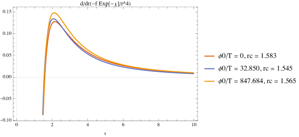
Figure 3: Plot for $\frac{d}{dr}\quantity(\frac{-fe^{-\chi}}{r^{4}})$ versus $r$, where we use $\rho=2$, $\gamma=0.2$, $\zeta=0.3$, and $n=1$. The root of this plot corresponds to the critical radius $r_{c}$. As one can see, the root lies not far from the horizon $r_{h}=1$.

From this idenfitication, we can plot the value of the Lyapunov exponent $\lambda_{L}$ as a function of the deformation parameter $\phi_{0}/T$. We only care about the behavior of the Lyapunov exponent as a function of $\phi_{0}$, i.e., whether it increases or decreases compared to both $\kappa$ and the aRN value $\lambda_{L_{\text{aRN}}}$ and not on the actual value of the Lyapunov exponent. Therefore, we plot the ratio between the Lyapunov exponent and the surface gravity and also the ratio between $\lambda_{L}$ and $\lambda_{L_{\text{aRN}}}$ versus the boundary deformation parameter $\phi_{0}/T$. The aRN Lyapunov exponent can be taken to be

$$\lambda_{L_{\text{aRN}}}=\frac{2}{\mathcal{N}_{\text{aRN}}}\quantity[\frac{1}{r_{c}^{4}}\quantity(1-\frac{r_{c}^{3}}{r_{h}^{3}}-\frac{r_{c}^{2}\zeta^{2}}{2}+\frac{r_{c}^{3}\zeta^{2}}{2r_{h}}+\frac{r_{c}^{4}\rho^{2}}{4}-\frac{r_{c}^{3}r_{h}\rho^{2}}{4})]^{1/2},$$ (59)

where $\mathcal{N}_{\text{aRN}}$ is the aRN version of the normalization constant to ensure $\lambda_{L}(\phi_{0}\rightarrow 0)=\lambda_{L_{\text{aRN}}}$. In the aRN case, the critical radius $r_{c}$ satisfy

$$-\frac{4}{r_{c}^{5}}+\frac{\zeta^{2}}{r_{c}^{3}}+\frac{\rho^{2}r_{h}^{4}-2\zeta^{2}r_{h}^{2}+4}{4r_{c}^{2}r_{h}^{3}}=0.$$ (60)

In finding the critical radius $r_{c}$ for calculating the Lyapunov exponent $\lambda_{L}$, we use the function FindRoot in Mathematica to find the root around the horizon. As one can see in Fig. 3, we can expect to not find another root in the deep interior since the graph asymptotes to zero in large $r$. However, one might anticipate that $r_{c}\rightarrow\infty$ also corresponds to

$$\frac{d}{dr}\quantity(\frac{fe^{-\chi}}{r^{4}})\bigg{|}_{r=r_{c}}\rightarrow 0,$$ (61)

and hence, taking the limit $r_{t}$ to be very close to the singularity will also render $\alpha\rightarrow\infty$. We will get back to this limit later, but for now, we focus on calculating $\lambda_{L}$ for $r_{c}$ near the horizon.
In this work, we consider only small value of the parameters $\zeta$ and $\gamma$. We also consider weak interaction between the gauge field $A_{\mu}$ and the scalar field $\phi$ by setting $q=0.005$ throughout numerical calculations since we would like to focus on varying the parameters $\zeta$ and $\gamma$, as well as the charge density $\rho$, which plays an important role in the charged hairy black hole geometry.

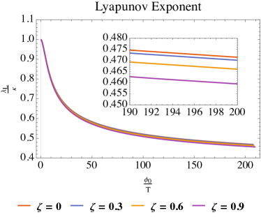
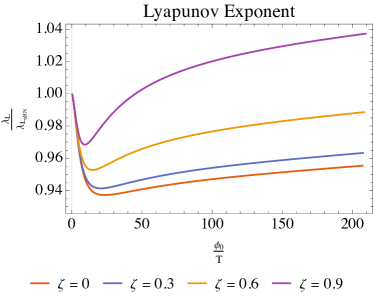
Figure 4: Ratio of the Lyapunov exponent $\lambda_{L}$ and the surface gravity $\kappa$ versus the dimensionless deformation parameter $\phi_{0}/T$ (left) and the Kasner exponent $p_{t}$ (right) for various value of the axion field parameter $\lambda$.

We plot the ratio $\lambda_{L}/\kappa$ and $\lambda_{L}/\lambda_{L_{\text{aRN}}}$ with respect to the boundary deformation parameter $\phi_{0}/T$ to see how boundary deformation affect the Lyapunov exponent of the black hole. The ratio $\lambda_{L}/\kappa$ decreases monotonically as the deformation parameter $\phi_{0}/T$ increases, as can be seen in Figure 4 (left). We can justify this plot by noticing that $T\rightarrow 0$ in the limit $\phi_{0}/T\rightarrow\infty$. This limit corresponds to extremal black hole with zero temperature which also have vanishing Lyapunov exponent (see [18, 19]). This also means that the Lyapunov exponent $\lambda_{L}$ approaches zero faster than the surface gravity $\kappa$ in the limit $T\rightarrow 0$. We cannot definitively conclude that $\lambda_{L}/\kappa$ approaches zero in the large $\phi_{0}/T$ limit, as our numerical calculations are finite. However, we observe from our plot that it becomes smaller as $\phi_{0}/T$ increases. In this plot, the axion parameter makes the vanishing property even faster as $T\rightarrow 0$.
On the other hand, the ratio $\lambda_{L}/\lambda_{L_{\text{aRN}}}$ does not have monotonic behavior, as can be seen in Figure 4 (right). It decreases at first, and start to increase after some value of $\phi_{0}/T$. At some point, when $\zeta=0.9$ for example, the ratio is greater than one, meaning that charged hairy black hole can be more chaotic than the aRN black hole. We also anticipate that as the deformation grows, the charged hairy black hole will eventually become more chaotic than the aRN black hole. Moreover, the axion parameter $\zeta$ appears to play a role in enhancing the chaotic behavior. The physics underlying this non-monotonic behavior remains unclear, as our results are based on numerical calculations. An analytical investigation, particularly through solving the equations of motion, is needed to provide a more detailed analysis of this behavior.
We also study the dependence of the Lyapunov exponent $\lambda_{L}$ on the Kasner exponent $p_{t}$ to gain insights into the geometry of the black hole interior and its relationship with boundary observables. The plot of $\lambda_{L}/\kappa$ and $\lambda_{L}/\lambda_{L_{\text{aRN}}}$ versus $p_{t}$ can be seen in Figure 5. Both figures show non-invertible relation between $\lambda_{L}$ and $p_{t}$. This is already anticipated as the behavior of the scrambling time $t_{*}$ and the butterfly velocity $v_{B}$ for neutral hairy black hole also exhibits similar result [28]. The non-invertible relation indicates that we cannot fully describe the interior geometry from boundary data alone and the Lyapunuov exponent is no exception. Other than that, we are interested in how the parameters $\zeta,\gamma$, and $\rho$ affect the relation between $\lambda_{L}$ and $p_{t}$.
Recall that the logarithmic behavior of $\phi$ at large $r$ in Eq. (32) can be derived from the equations of motion for $\zeta,\gamma=0$. We are interested in whether the relation between $\lambda_{L}$ and $p_{t}$ is still the same if we increase $\zeta,\gamma,\rho$. The result of varying $\zeta$ can be seen in Figure 5. The relationship between $\lambda_{L}/\kappa$ and $p_{t}$ behaves normally when we increase $\zeta$, as $\zeta$ increases the value of $p_{t}$ for same $\lambda_{L}/\kappa$. In contrast, the behavior of $\lambda_{L}/\lambda_{L_{\text{aRN}}}$ as a function of $p_{t}$ reveals an interesting pattern: at small $\zeta$, the curves closely resemble the $\zeta=0$ case. However, as $\zeta$ increases, the behavior of the plot begins to deviate. For $\zeta=0$ and $\zeta=0.3$, the curves curl down as the boundary deformation increases. However, for $\zeta=0.6$ and $\zeta=0.9$, the curves curl up, enlarging the ratio $\lambda_{L}/\lambda_{L_{\text{aRN}}}$. This shows us how $\zeta$ affect the interior Kasner solution although $rd\phi/dr$, as can be seen in Figure 2, does not get affected much by the variation of $\zeta$.

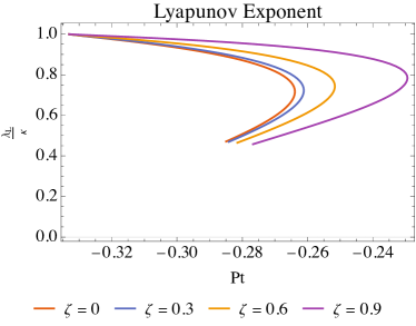
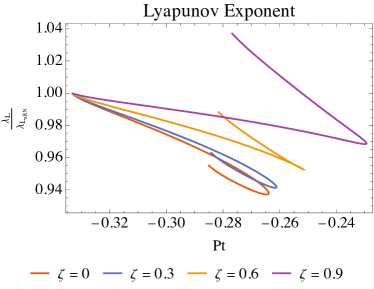
Figure 5: Ratio of the Lyapunov exponent $\lambda_{L}$ and the surface gravity $\kappa$ versus the dimensionless deformation parameter $\phi_{0}/T$ (left) and the Kasner exponent $p_{t}$ (right) for various value of the axion field parameter $\lambda$.

The behavior of $\lambda_{L}/\kappa$ and $\lambda_{L}/\lambda_{L_{\text{aRN}}}$ vs. $\phi_{0}/T$ as we vary $\gamma$ can be seen in Figure 6. In general, the result gives us similar conclusions. However, in contrast with the $\zeta$ variation result, as we increase $\gamma$, the ratio $\lambda_{L}/\kappa$ decreases. On the other hand, the behavior of $\lambda_{L}/\lambda_{L_{\text{aRN}}}$ is quite different. Initially, for small enough $\phi_{0}/T$, the parameter $\gamma$ decreases the ratio $\lambda_{L}/\lambda_{L_{\text{aRN}}}$. After reaching a certain value of $\phi_{0}/T$, it causes the ratio to increase. We do not see the case where the ratio $\lambda_{L}/\lambda_{L_{\text{aRN}}}$ is greater than one. Nevertheless, we expect it to keep increasing as $\phi_{0}/T$ becomes larger and eventually surpass unity.

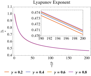
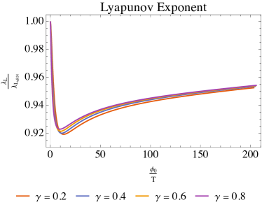
Figure 6: Ratio of the Lyapunov exponent $\lambda_{L}$ and the surface gravity $\kappa$ versus the dimensionless deformation parameter $\phi_{0}/T$ (left) and the Kasner exponent $p_{t}$ (right) for various value of the axion field parameter $\lambda$.

For the relationship of $\lambda_{L}/\kappa$ vs. $p_{t}$, we do not see anything new when we vary $\gamma$, as can be seen in Figure 7. However, the plot of $\lambda_{L}/\lambda_{L_{\text{aRN}}}$ vs. $p_{t}$ shows something unique. It curves upward for all values of $\gamma>0$ and shows an inverted behavior after a certain turning point. Initially, increasing $\gamma$ reduces the ratio $\lambda_{L}/\lambda_{L_{\text{aRN}}}$, but after reaching a turning point that corresponds to a specific deformation $\phi_{0}/T$, increases in $\gamma$ cause the ratio to rise. This shifting behavior after some turning point is again unique to the Einstein-Maxwell coupling constant $\gamma$. This distinct behavior after we turned on $\gamma$ is also present in [26] when investigating the interior structure of the holographic superconductor since for large enough $\gamma$, the terms that contains $\gamma$ in the equations of motion becomes more important as we go deeper into the interior.

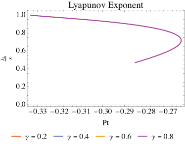
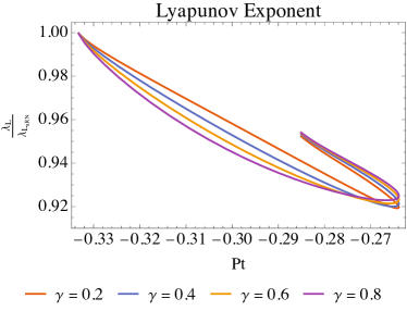
Figure 7: Ratio of the Lyapunov exponent $\lambda_{L}$ and the surface gravity $\kappa$ versus the dimensionless deformation parameter $\phi_{0}/T$ (left) and the Kasner exponent $p_{t}$ (right) for various value of the axion field parameter $\lambda$.

Aside from varying $\zeta$ and $\gamma$, we also vary the charge density $\rho$. Previous calculations involve constant charge density $\rho=2$. In this part, we vary $\rho$ from 0.5 to 2, as can be seen in Figure 8 and Figure 9. Again, the plot of $\lambda_{L}/\kappa$ and $\lambda_{L}/\lambda_{L_{\text{aRN}}}$ versus the boundary deformation parameter $\phi_{0}/T$ shows similar result, as increasing $\rho$ opts to decreasing both ratios. For the relation with Kasner exponent $p_{t}$, Figure 9 shows the curl-down behavior of the ratio $\lambda_{L}/\lambda_{L_{\text{aRN}}}$ up until $\rho=2$. This also indicate that the behavior of the plot behaves differently when $\rho$ becomes quite large, similar with other parameters $\zeta$ and $\gamma$. Finally, we summarize the effect of the parameters $\zeta,\gamma,\rho$ to the ratios $\lambda_{L}/\kappa$ and $\lambda_{L}/\lambda_{L_{\text{aRN}}}$ in Table 1.

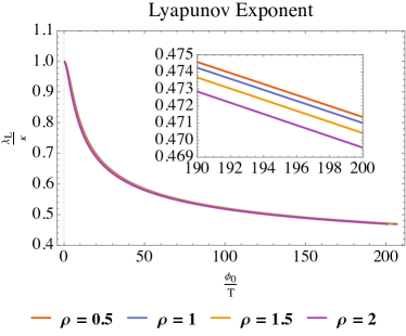
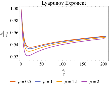
Figure 8: Ratio of the Lyapunov exponent $\lambda_{L}$ and the surface gravity $\kappa$ versus the dimensionless deformation parameter $\phi_{0}/T$ (left) and the Kasner exponent $p_{t}$ (right) for various value of the axion field parameter $\lambda$.

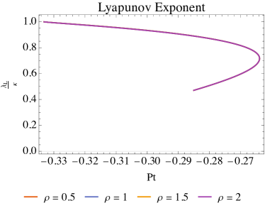
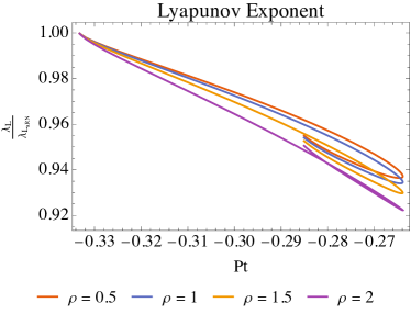
Figure 9: Ratio of the Lyapunov exponent $\lambda_{L}$ and the Lyapunov exponent of an aRN black hole $\lambda_{L_{\text{aRN}}}$ versus the dimensionless deformation parameter $\phi_{0}/T$ (left) and the Kasner exponent $p_{t}$ (right) for various value of the axion field parameter $\lambda$.

	Increase in $\zeta$	Increase in $\gamma$	Increase in $\rho$
$\lambda_{L}/\kappa$	Decrease	Decrease–Increase	Decrease
$\lambda_{L}/\lambda_{L_{\text{aRN}}}$	Increase	Decrease–Increase	Decrease

Table 1: Summary of the behavior of the Lyapunov exponent ratios $\lambda_{L}$ for some value of boundary deformation $\phi_{0}/T$ under variations of $\zeta$, $\gamma$, and $\rho$. Decrease–Increase means that the ratio decreases before the turning point and increases afterwards.

Our result so far indicates that the Lyapunov exponent, being some quantities from the boundary theory, cannot completely determine Kasner geometry in the interior of the black hole since the relation is not invertible. This is so even though in calculating the Lyapunov exponent, we involve the calculation of the mutual information $I(A;B)$ that comes from the entangling Hartman-Maldacena surface that slightly penetrates the interior at $r=r_{c}$. Other quantity such as the subleading term near the singularity is needed to completely reconstruct interior geometry in terms of boundary data. Nevertheless, we obtain some important information on how the parameters $\zeta,\gamma,\rho$ affects the ratio of the Lyapunov exponent.

III.3 Near-Singularity Area Functional

To learn more about physics near the singularity in terms of the mutual information $I(A;B)$, we also calculate the area functional $\mathcal{A}$ defined in Eq. (40), as $r_{t}\rightarrow\infty$. In this limit, the conserved quantity $K$ approaches zero, as well as the boundary time $t_{b}$ from Eq. (42).
From Eq. (41), and the near-singularity expansions of $f$ and $\chi$, we obtain the relation between the turning point $r_{t}$ and $K$, as $r_{t}\rightarrow\infty$,

$$r_{t}=\quantity(\frac{f_{K1}e^{-\chi_{K1}}}{K^{2}})^{\frac{1}{1+c^{2}}}+...\;,$$ (62)

where $...$ denotes subleading terms as $K\rightarrow 0$. Using this relation, the area functional then becomes

$$\mathcal{A}=L_{y}\int dr\frac{1}{\sqrt{-f_{K1}}r^{(7+2c^{2})/2}}\quantity[1-\quantity(\frac{K^{2}}{f_{K1}e^{-\chi_{K1}}})r^{1+c^{2}}]^{1/2},$$ (63)

in one of its end point near the singularity. This integral can be calculated explicitly using binomial expansion and it gives us

$$\mathcal{A}=\tilde{l}K^{\frac{2c^{2}+5}{c^{2}+1}},$$ (64)

where $\tilde{l}$ is a constant that depends on $L_{y}$ and other near-singularity data such as $f_{K1},\chi_{K1},c$ and does not depends on $K$. This term of the area functional approaches zero as $K\rightarrow 0$.
Aside from this endpoint, we also need to calculate the area functional in the other endpoint which is closer to the boundary. Although it depends on boundary data such as $\phi_{0},\expectationvalue{\mathcal{O}},\expectationvalue{T_{tt}}$, it only depends linearly on $K$ and thus also vanish in $K\rightarrow 0$ limit. The explicit calculation for both endpoints after we subtract the universal divergent part gives us

$$\mathcal{A}=lK+...+\tilde{l}K^{\frac{2c^{2}+5}{c^{2}+1}}+...\;,$$ (65)

where $l$ depends on the entire flow from the boundary to the singularity. The vanishing area functional $\mathcal{A}$ indicates the time scale where the mutual information $I(A;B)$ is still large and thus the OTOC is also still large. In this time scale, we do not expect to observe any exponential decay behavior of the OTOC, and thus it may not be suitable for extracting information about the chaotic properties of the system. However, since this area penetrates deep in the interior, we expect to see something interesting about its relation to the emergence of Kasner spacetime. Future investigations, including more rigorous analytical analyses, may shed further light on these aspects.

III.4 Localized Chaos and Butterfly Velocity

In this section, we find out how the parameters $\zeta,\gamma,\rho$ affect the buttefly velocity as a function of both boundary deformation $\phi_{0}/T$ and Kasner exponent $p_{t}$. If the gravitational shock waves is sent from the left boundary at some local point in space, the shock wave parameter $\alpha$ depends locally on position coordinate $x,y$ and propagates in a null path at $U=0$. For simplicity, we may assume that the gravitational shock waves function is in the form of $\delta(\vec{x})$. For large insertion time $t_{w}$, the gravitational shock waves is boosted as it approach the black hole horizon and the stress-energy tensor is given by

$$T_{UU}^{\text{shock}}=Ee^{\frac{2\pi t_{w}}{\beta}}\delta(U)\delta(\vec{x}).$$ (66)

The gravitational shock waves perturbs the background geometry as $dV\rightarrow dV+\delta(U)\alpha(x)dU$, giving us the Dray-’t Hooft solution. Plugging in this solution to the Einstein’s equation with $T_{UU}^{\text{shocks}}$ gives us (see [28] for more detailed expressions)

$$\alpha(x)=\frac{e^{\frac{2\pi}{\beta}\quantity((t_{w}-t_{*})-\frac{|x|}{v_{B}})}}{|x|^{1/2}},$$ (67)

where

$$v_{B}=\sqrt{\pi Tr_{h}e^{-\chi_{h}/2}},$$ (68)

is defined as the butterfly velocity.
Again, this butterfly velocity is influenced by the boundary deformation through the function $\chi$. The Schwarzschild value of the butterfly velocity is $v_{B}=\sqrt{3}/2$. We normalize our calculations with respect to the Schwarzschild value so that it reduces to one when both the axion paramater $\zeta$ and the boundary deformation $\phi_{0}$ vanish. The dependence on the butterfly velocity with the boundary deformation parameter $\phi_{0}/T$ can be seen in Figure 10. It shows non-monotonic behavior that decrease first before the turning point and increase afterward. We see that the axion parameter $\zeta$ decreases the butterfly velocity and this also the case when there is no boundary deformation. The presence of EMS coupling $\gamma$ reduces the butterfly velocity before the turning point but increases it afterward. The charge density $\rho$, similar with the axion parameter $\zeta$, decreases the butterfly velocity. Although the curves shows similar form with the Lyapunov exponent, it turns out that the effect on the parameters $\zeta,\gamma,\rho$, especially the axion parameter, is quite different.

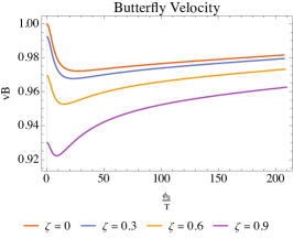
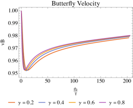
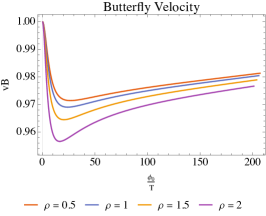
Figure 10: Plot of the butterfly velocity $v_{B}$ versus the boundary deformation $\phi_{0}/T$ (left) and the Kasner exponent $p_{t}$ (right). The butterfly velocity is normalized with respect to its aRN value.

The effect on the parameters $\zeta,\gamma,\rho$ to the plot of $v_{B}$ versus $p_{t}$ can be seen in Figure 11. All plots show non-invertible behavior, as the butterfly velocity cannot fully determine the interior geometry of the black hole. What interesting here is that the parameters shift the behavior of the curve. For large enough $\zeta$, the curves curl upwards instead of downwards like the $\zeta=0$ case. We also see this behavior when the charge density $\rho$ is varied. All of the curves curl upward when the EMS parameter $\gamma$ is turned on. The presence of these parameters, in general, reduces the value of the butterfly velocity. This means that the shock wave perturbation spread more slowly when these parameters are turned on. We also do not see the case where the butterfly velocity becomes larger than its Schwarzschild value, although we might expect this to happen when $\phi_{0}/T$ becomes very large. However, as $T\rightarrow 0$, we expect the butterfly velocity to vanish as in this temperature, the perturbation would not spread. This can also be expected from the fact that the butterfly velocity explicitly depends on the temperature as can be seen in Eq. (68). Further analytical analysis will help us to understand this limit better.

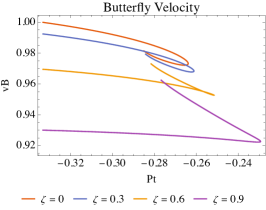
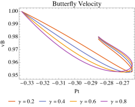
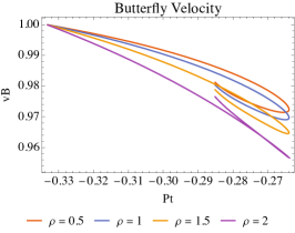
Figure 11: Plot of the butterfly velocity $v_{B}$ versus the boundary deformation $\phi_{0}/T$ (left) and the Kasner exponent $p_{t}$ (right). The butterfly velocity is normalized with respect to its aRN value.

III.5 Shock Wave Bounce in the Interior and Scrambling Time Delay

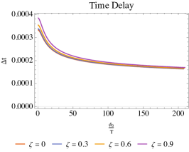
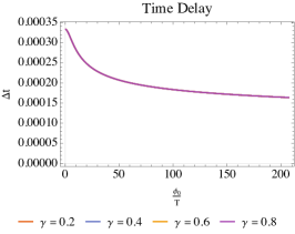
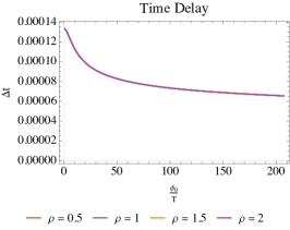
Figure 12: The plot of time delay $\Delta t$ vs. boundary deformation parameter $\phi_{0}/T$ by varying parameters $\zeta$ (left), $\gamma$ (center), and $\rho$ (right). In this plot, we use $\mathcal{Q}=0.2$.

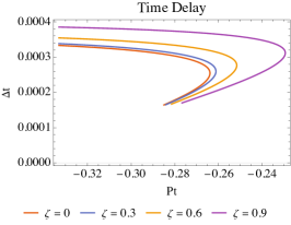
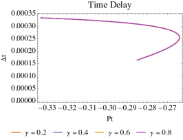
Figure 13: The plot of time delay $\Delta t$ vs. Kasner exponent $p_{t}$ by varying parameters $\zeta$ (left), $\gamma$ (center), and $\rho$ (right). In this plot, we use $\mathcal{Q}=0.2$.

Since we perturb our black hole by charged shock waves instead of neutral one, we may expect bouncing in the interior as first explained in [15]. This bounce happens so that the null energy condition is not violated. We are particularly interested in investigating this bounce and its relation to the boundary deformation and the Kasner exponents, as this bounce also occurs in the interior, albeit near the horizon.
The mutual information $I(A;B)$ in Eq. (54) vanishes when the insertion time $t_{w}$ is given by

$$\kappa t_{*}=\log S+\frac{(\mathcal{A}_{A}+\mathcal{A}_{B})}{4\pi\sqrt{-f(r_{c})e^{-\chi(r_{c})}/r_{c}^{4}}}+\log\frac{1}{1-\Phi_{h}\mathcal{Q}}.$$ (69)

This time scale $t_{*}$ is defined as the scrambling time. The first term indicates that the system is fast scrambling, while the second term can be neglected in the large $S$ limit since it does not scale as the entropy. The last term comes from the interaction between the shock wave charge per unit of energy $\mathcal{Q}$ and the black hole’s electric potential $\Phi_{h}$, which is the potential $\Phi(r)$ located at the horizon, i.e. $\Phi_{h}=\Phi(r_{h})$. When either shock wave’s or black hole’s charge vanishes, this term also vanishes. Recent work [15] shows that the last term corresponds to the delay of the scrambling process, instead of prolonging the scrambling time.
Since the electric potential $\Phi(r)$ interacts with the scalar field $\phi(r)$ in the bulk, then this time delay term, which we denote as

$$\Delta t=\frac{1}{\kappa}\log\frac{1}{1-\Phi_{h}\mathcal{Q}},$$ (70)

also gets affected by the boundary deformation parameter $\phi_{0}/T$. The plot of the time delay $\Delta t$ versus the boundary deformation can be seen in Figure 12. The time delay $\Delta t$ decreases monotonically as we increase $\phi_{0}/T$. The decreasing behavior of this time delay means that the logarithmic term goes to zero faster than the surface gravity $\kappa$ when $\phi_{0}/T$ gets larger. This logarithmic term is controlled solely by the electric potential $\Phi(r_{h})$. The axion parameter $\zeta$ slightly increases the time delay, while it seems constant with respect to parameters $\gamma$ and $\rho$. We can also see how the time delay is related to the Kasner exponent from Figure 13.

IV What Happens after Kasner Inversion/Transition?

Although the value of $r\phi^{\prime}/\sqrt{2}$ remains approximately constant for large value of $r$, there is a radial location $r_{\text{inv}}$ where the value of $r\phi^{\prime}/\sqrt{2}$ changes at $r\approx r_{\text{inv.}}$. For example, in Figure 14, at around $r_{\text{inv.}}\sim 10^{8}$, the value of $c$ is inverted as

$$\frac{r\phi^{\prime}}{\sqrt{2}}\rightarrow c_{1},\;\;\;1\ll r\ll r_{\text{inv.}};\;\;\;\frac{r\phi^{\prime}}{\sqrt{2}}\rightarrow c_{2}\approx\frac{1}{c_{1}},\;\;\;r\gg r_{\text{inv.}}.$$ (71)

This phenomenon is called the Kasner inversion [26, 27]. In this section, we would like to see what happens to the boundary values such as the Lyapunov exponent, butterfly velocity, and scrambling time delay, when we vary the parameters $\zeta,\gamma,\rho$ after Kasner transition. Therefore, there are two Kasner geometries inside the horizon with two different Kasner exponents. We use $r=1000$ to obtain the first constant $c_{1}$ while $r=10^{14}$ to obtain the second constant $c_{2}$ in the numerical calculations.
The axion parameter $\zeta$ increases the value of $c_{1}$, while it decreases the value of $c_{2}$, as expected from the inversion since we have $c_{2}\approx\frac{1}{c_{1}}$. An interesting thing to note is that the difference between $c_{2}$ and $\frac{1}{c_{1}}$ increases as the axion parameter $\zeta$ increases, which can be seen in Figure 15. The difference increases linearly around $\zeta=0.3$ to $\zeta=0.7$, which indicates that the inversion phenomena drifts away from the notion of ”inversion” as $\zeta$ increases. Since $c_{1}$ is smaller than 1, the Kasner exponent is always negative-valued. However, this means that the value of $c_{2}$ is larger than one, which makes the Kasner exponent positive. We may anticipate dramatic changes when the boundary deformation $\phi_{0}$ is turned on since it change $p_{t}$ from Schwarzschild value of -1/3 to some positive value afterwards.

Figure 14: Plot for $r\phi^{\prime}/\sqrt{2}$ versus $r$. Left: the value of $r\phi^{\prime}/\sqrt{2}$ that stretches from the asymptotic boundary all the way to $r=10^{18}$, which is beyond the transition point. Center: The zoomed-in version on the first Kasner regime. Right: The zoomed-in version on the Kasner regime after inversion. We vary the value of $\zeta=\{0,0.3,0.6,0.9\}$.

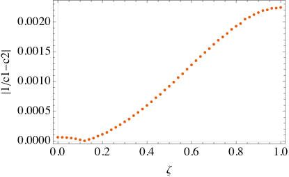
Figure 15: Difference between $c_{2}$ and $\frac{1}{c_{1}}$ as a function of $\zeta$.

The plot of the Lyapunov exponent ratios $\lambda_{L}/\kappa$ and $\lambda_{L}/\lambda_{L_{\text{aRN}}}$, butterfly velocity $v_{B}$, and time delay $\Delta t$ with respect to Kasner exponent $p_{t}$ after inversion, as we vary $\zeta$, can be seen in Figure 16. The values of $\{\lambda_{L}/\kappa,\lambda_{L}/\lambda_{L_{\text{aRN}}},v_{B},\Delta t\}$ are all sensitive to the change in $\zeta$ after Kasner inversion. In those cases, the values of the Kasner exponents are all positive. Our numeric breakdown occurs when the Kasner exponent undergoes a dramatic change from -1/3 to 1 right after we turned on the boundary deformation $\phi_{0}$. However, it went smoothly again after some time, when $\phi_{0}/T$ becomes large enough. The behavior of the curves are all similar to the cases before the inversion, although in this case, they are mirrored. The parameter $\zeta$ decreases the Kasner exponent $p_{t}$ for the same value of $\lambda_{L}/\kappa$, $\lambda_{L}/\lambda_{L_{\text{aRN}}}$, $v_{B}$, and $\Delta t$.

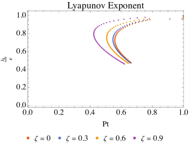
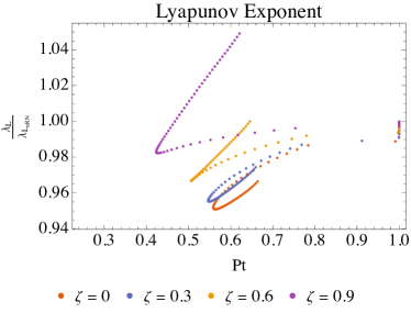
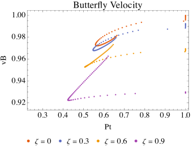
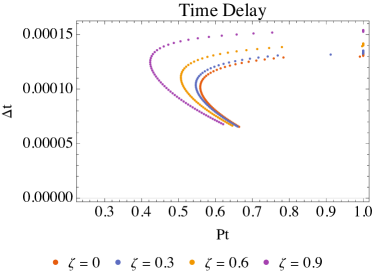
Figure 16: The boundary parameters $\lambda_{L}/\kappa$ (upper left), $\lambda_{L}/\lambda_{L_{\text{aRN}}}$ (upper right), $v_{B}$ (lower left), and $\Delta t$ (lower right) as a function of the Kasner exponent $p_{t}$ after Kasner inversion. The axion parameter $\zeta$ is varied as $\zeta=\{0,0.3,0.6,0.9\}$.

Quite contrary to the previous case, when the parameter $\gamma$ is turned on, the second Kasner regime emerges not as an inversion, but rather as a transition since $c_{2}\neq\frac{1}{c_{1}}$, as can be seen in Figure 17. The parameter $\gamma$ only slightly reduces the value of $c_{2}$ after transition. However, there is a significant gap between $\gamma=0$ and $\gamma>0$ case. This transition behavior when the parameter $\gamma$ is turned on is also present in [26]. In this work, we can also see how this transition affect the dependence of the boundary parameters $\{\lambda_{L}/\kappa,\lambda_{L}/\lambda_{L_{\text{aRN}}},v_{B},\Delta t\}$ with the Kasner exponent $p_{t}$, as can be seen in Figure 18. The gap between $\gamma=0$ and $\gamma>0$ cases are clearly visible, although the parameter $\gamma$ only slightly changes the curves after it is turned on.
We also observe that the charge density $\rho$ does not affect the regions after Kasner inversion, and therefore, we do not put them here for brevity. It is the parameters $\zeta$ and $\gamma$ that play important role after Kasner inversion/transition.
Note that all of the parameters $\{\lambda_{L}/\kappa,\lambda_{L}/\lambda_{L_{\text{aRN}}},v_{B},\Delta t\}$ only depends on the radius that is located not far from the horizon, although it is in the interior of the black hole. For instance, the Lyapunov exponent depends on the critical radius $r_{c}$, which has been shown earlier, does not penetrates far from the horizon. The butterfly velocity and the scrambling time delay $\Delta t$ also depends on the horizon radius. Therefore, it does not get affected much if we consider regions after Kasner inversion/transition. Nevertheless, the inversion/transition effect are visible from the relation between the boundary parameters with the Kasner exponent $p_{t}$.

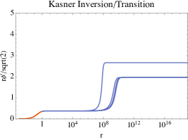
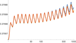
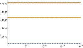
Figure 17: Kasner transition occur after $r\approx r_{\text{inv.}}$ when the parameter $\gamma$ is turned on. The parameter $\gamma$ is varied as $\gamma=\{0,0.2,0.4,0.6,0.8\}$.

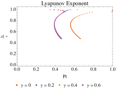
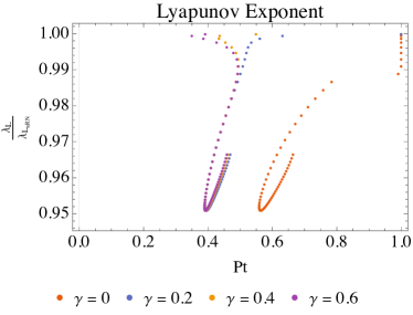
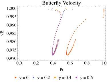
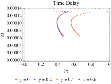
Figure 18: The boundary parameters $\lambda_{L}/\kappa$ (upper left), $\lambda_{L}/\lambda_{L_{\text{aRN}}}$ (upper right), $v_{B}$ (lower left), and $\Delta t$ (lower right) as a function of the Kasner exponent $p_{t}$ after Kasner inversion. The EMS coupling constant $\gamma$ is varied as $\gamma=\{0,0.2,0.4,0.6\}$.

V Summary and Discussions

In this work, we study how chaotic parameters such as the quantum Lyapunov exponent $\lambda_{L}$, the butterfly velocity $v_{B}$ and the scrambling time delay $\Delta t$ are affected by the deformation $\phi_{0}$ that renders a more general Kasner geometry in the interior of a charged hairy black hole. Those boundary parameters are obtained after we inject charged gravitational shock waves into the black hole, that gets highly blueshifted as they enter the black hole horizon. Our goal is to study how the boundary parameters can gives us insight about the interior Kasner geometry through they relation with Kasner exponents. We consider a more general charged hairy black hole with axion parameter $\zeta$ and EMS coupling $\gamma$ that generates a coupling term $F_{\mu\nu}F^{\mu\nu}|\phi|^{2}$. The bulk scalar field $\phi(r)$ also interacts with bulk Maxwell field $A_{\mu}$ with charge density $\rho$.
We calculate the Ryu-Takayanagi minimal surfaces that stretch from the left asymptotic boundary to the right one to calculate the holographic mutual information $I(A;B)$ in the scrambling regime. This mutual information is then used to obtain the quantum Lyapunov exponent $\lambda_{L}$ and extract the scrambling time delay $\Delta t$. It is important to note that such a minimal surface penetrates the black hole horizon and thus parts of them lies in the interior of the black hole. Therefore, it is natural to expect a non-trivial relation between the quantum Lyapunov exponent as a boundary data to the Kasner geometry in the interior of the black hole. We first study how the boundary deformation $\phi_{0}$ affects the boundary parameters $\{\lambda_{L}/\kappa,\lambda_{L}/\lambda_{L_{\text{aRN}}},v_{B},\Delta t\}$. Our solutions are normalized so that, when the boundary deformation is absent, they reduce to the axion-Reissner-Nordström (aRN) solution.
We find that the Lyapunov exponent ratio $\lambda_{L}/\kappa$ decreases monotonically as we increase $\phi_{0}/T$, while the ratio $\lambda_{L}/\lambda_{L_{\text{aRN}}}$ shows non-monotonic behavior. Since, at some point, the ratio $\lambda_{L}/\lambda_{L_{\text{aRN}}}$ can be greater than one, we can conclude that the boundary deformation can make the black hole more chaotic than the aRN case while still obeying the MSS chaos bound. The axion parameter $\zeta$ decrease the ratio $\lambda_{L}/\kappa$ while it increase the ratio $\lambda_{L}/\lambda_{L_{\text{aRN}}}$ while the charge density $\rho$ decreases both ratios. Interestingly, the EMS coupling term shows a transition, i.e. it decreases the ratios first, then increasing them after some turning point. We also show that the Lyapunov exponent $\lambda_{L}$ approaches zero faster than the surface gravity $\kappa$ as the parameter $\phi_{0}/T\rightarrow\infty$. This is as expected if such a limit is obtained from $T\rightarrow 0$ limit since the Lyapunov exponent should vanish in zero temperature limit. However, we should also consider the effect of large boundary deformation parameter $\phi_{0}$. Our numerical calculations are limited in determining exactly what happens in this limit and thus further analytical calculations are required. We also observe relations between the Lyapunov exponent ratios with the Kasner exponent $p_{t}$. In these cases, the relations are non-invertible, meaning that we can have two different values of the Lyapunov exponent ratios for each value of $p_{t}$. This result is also expected from [28] and we can conclude that boundary data alone, although some of them are located in the interior of the black hole, are not sufficient to fully determine the Kasner geometry near the singularity. We expect subleading expansion near the singularity is required.
We also calculate the RT minimal surface that penetrates deeper into the horizon, by taking the limit $r_{t}\rightarrow\infty$, i.e. the minimal surfaces have turning point very close to the singularity. Previously, [28, 25] calculate the geodesic length, instead of a codimension two minimal surface, in this limit as well. In contrast with the geodesic length calculation, the area functional approaches zero in this limit, although it is still depends on some boundary data such as $\phi_{0},\expectationvalue{\mathcal{O}},\expectationvalue{T_{tt}}$. The vanishing feature of the minimal surface corresponds to the boundary time scale where the mutual information $I(A;B)$ is still large (with only small contribution from $S_{A\cup B}$) and hence the OTOC is also still large. In this time scale, we cannot extract the chaotic behavior of the system since the chaotic regime happens at time scale much larger than the thermal time $\beta$. We can make some important comments here. To fully reconstruct the bulk geometry from these minimal surfaces, we need all surfaces from all boundary time, ranging from zero to infinity. At large time scale, chaotic behavior happens and hence the boundary data such as the Lyapunov exponent, butterfly velocity, and the scrambling time delay play an important role here. However, we also need to study the behavior of the OTOC, or the mutual information, during earlier period, when the chaotic behavior is not yet present. We expect future works in this direction will give us more insight in studying the interior part of a hairy black hole.
The butterfly velocity $v_{B}$ also gets affected by the boundary deformation. It shows non-monotonic behavior as we increase $\phi_{0}/T$. The butterfly velocity, for all cases, are smaller than the Schwarzschild value $v_{B}=\sqrt{3}/2$. However, we cannot conclude whether $v_{B}$ vanishes or gets back to its Schwarzschild value when $\phi_{0}/T\rightarrow\infty$, although, since it depends explicitly on the black hole temperature, it should goes to zero as $T\rightarrow 0$. The axion parameter $\zeta$ and the charge density $\rho$ decreases the butterfly velocity, while the EMS coupling constant $\gamma$ gives us transitional behavior. The relation between $v_{B}$ and $p_{t}$ also gives us non-invertible relation as the butterfly velocity cannot fully determine the interior geometry as well. What interesting here is that the behavior of the curves changes for large values of $\zeta$ and $\rho$, from curling down to curling up. The EMS parameter $\gamma$ also gives us transitional behavior in this case.
The scrambling time $t_{*}$ gets a contribution that depends on the interaction between black hole’s electric potential $\Phi_{h}$ and the shock waves charge $\mathcal{Q}$. This term was first studied in [15] and corresponds to the scrambling time delay. We study how the parameters $\zeta,\gamma,\rho$ affects this time delay and its relation with the boundary deformation parameter $\phi_{0}/T$ and the Kasner exponent $p_{t}$. The time delay decreases monotonically as we increase the boundary deformation parameter. The axion parameter $\zeta$ slightly increasaes $\Delta t$, while other parameters $\gamma$ and $\rho$ does not significantly affect the time delay. The effect of the axion parameter $\zeta$ also clearly visible in the relation between $\Delta t$ and $p_{t}$, as it increases the Kasner exponent for the same value of $\Delta t$.
Due to the existence of the parameters $\zeta$ and $\gamma$, the interior geometry of charged hairy black hole can exhibit a Kasner inversion/transition, where the Kasner exponent changes after $r\approx r_{\text{inv.}}$ [26, 27]. It is called Kasner inversion when the integration constant $c$ is inverted to $1/c$ at $r\gg r_{\text{inv.}}$, while it is called Kasner transition when $c$ changes but not equal to $1/c$. The parameter $\zeta$ generates Kasner inversion, but it drifts away from the notion of inversion as $\zeta$ becomes larger. On the other hand, the EMS coupling $\gamma$ generates Kasner transition when it is turned on, and shows a significant gap between $\gamma=0$ and $\gamma>0$ cases. These behavior is also encoded in the relation between boundary chaotic parameters $\lambda_{L}/\kappa,\lambda_{L}/\lambda_{L_{\text{aRN}}},v_{B},\Delta t$ and the Kasner exponent $p_{t}$. Some remarks about regions after inversion/transition is that the boundary data only depends on a radial value that is not far from the horizon while the inversion radius $r_{\text{inv.}}$ is located deep in the interior with approximate value of $r_{\text{inv.}}\approx 10^{8}$. Therefore, we expect the area functional with $r_{t}\rightarrow\infty$ and physics underlying this time scale will give us more insight from the region after Kasner inversion/transition.
What interesting to explore next is to study how rotating shock waves [16], or even rotating and charged shock waves [19], disrupt the rotating (and charged) hairy black holes [38] and how they affect the interior geometry. Furthermore, we are also interested in how this relevant deformation affects the traversability of a wormhole due to double-trace deformation in the boundary [40, 41]. This is interesting to explore since information traversing the wormhole also enters the interior before eventually coming out to the other region. Recently, the analytical solutions of scalar hair black holes was investigated in [42]. We hope this finding can help us in investigating the chaotic behavior in some certain limit (such as $T\rightarrow 0$ limit for example) of hairy black holes. We will explore these aspects in future works.

References

- [1] J. Maldacena, The Large N Limit of Superconformal Field Theories and Supergravity, Int. J. Theor. Phys. 38 (1999) 1113–1133. doi:https://doi.org/10.1023/A:1026654312961.
-
[2]
S. de Haro, K. Skenderis, S. N. Solodukhin,
Holographic
reconstruction of spacetime and renormalization in the ads/cft
correspondence, Communications in Mathematical Physics 217 (2001) 595–622.
arXiv:hep-th/0002230, doi:10.1007/s002200100381.
URL https://link.springer.com/article/10.1007/s002200100381 -
[3]
T. D. Jonckheere, Modave
lectures on bulk reconstruction in ads/cft, Proceedings of Science (PoS)
Modave2017 (2018) 005, lecture notes from the XIII Modave Summer School in
Mathematical Physics.
arXiv:arXiv:1711.07787, doi:10.48550/arXiv.1711.07787.
URL https://doi.org/10.48550/arXiv.1711.07787 -
[4]
S. Ryu, T. Takayanagi,
Holographic
Derivation of Entanglement Entropy from the anti–de Sitter Space/Conformal
Field Theory Correspondence, Phys. Rev. Lett. 96 (18) (2006) 181602.
doi:10.1103/PhysRevLett.96.181602.
URL https://link.aps.org/doi/10.1103/PhysRevLett.96.181602 - [5] S. Ryu, T. Takayanagi, Aspects of holographic entanglement entropy, J. High Energ. Phys. 08 (2006) 45. doi:https://doi.org/10.1088/1126-6708/2006/08/045.
- [6] T. Hartman, J. Maldacena, Time evolution of entanglement entropy from black hole interiors, Journal of High Energy Physics 2013 (5) (2013). doi:10.1007/JHEP05(2013)014.
- [7] S. H. Shenker, D. Stanford, Black holes and the butterfly effect, Journal of High Energy Physics 2014 (3) (2014). doi:10.1007/JHEP03(2014)067.
-
[8]
S. H. Shenker, D. Stanford,
Stringy effects in
scrambling, Journal of High Energy Physics 2015 (5) (2015) 132.
doi:10.1007/JHEP05(2015)132.
URL https://doi.org/10.1007/JHEP05(2015)132 -
[9]
D. A. Roberts, D. Stanford, L. Susskind,
Localized shocks, Journal of
High Energy Physics 2015 (3) (2015) 51.
doi:10.1007/JHEP03(2015)051.
URL https://doi.org/10.1007/JHEP03(2015)051 - [10] Y. Sekino, L. Susskind, Fast scramblers, Journal of High Energy Physics 2008 (10) (2008). doi:10.1088/1126-6708/2008/10/065.
- [11] J. Maldacena, S. H. Shenker, D. Stanford, A bound on chaos, Journal of High Energy Physics 2016 (8) (2016). doi:10.1007/JHEP08(2016)106.
- [12] S. Leichenauer, Disrupting entanglement of black holes, Physical Review D - Particles, Fields, Gravitation and Cosmology 90 (4) (2014). doi:10.1103/PhysRevD.90.046009.
- [13] V. Jahnke, Delocalizing entanglement of anisotropic black branes, Journal of High Energy Physics 2018 (1) (2018). doi:10.1007/JHEP01(2018)102.
- [14] V. Jahnke, K. Y. Kim, J. Yoon, On the chaos bound in rotating black holes, Journal of High Energy Physics 2019 (5) (2019). doi:10.1007/JHEP05(2019)037.
- [15] G. T. Horowitz, H. Leung, L. Queimada, Y. Zhao, Bouncing inside the horizon and scrambling delays, Journal of High Energy Physics 2022 (11) (2022). doi:10.1007/JHEP11(2022)025.
- [16] V. Malvimat, R. R. Poojary, Fast scrambling due to rotating shockwaves in BTZ, Physical Review D 105 (12) (2022). doi:10.1103/PhysRevD.105.126019.
- [17] V. Malvimat, R. R. Poojary, Fast scrambling of mutual information in Kerr-AdS5, Journal of High Energy Physics 2023 (3) (2023). doi:10.1007/jhep03(2023)099.
- [18] V. Malvimat, R. R. Poojary, Fast scrambling of mutual information in Kerr- AdS4 spacetime, Physical Review D 107 (2) (2023). doi:10.1103/PhysRevD.107.026019.
-
[19]
H. L. Prihadi, F. P. Zen, D. Dwiputra, S. Ariwahjoedi,
Chaos and fast
scrambling delays of a dyonic kerr-sen- black hole and
its ultraspinning version, Phys. Rev. D 107 (2023) 124053.
doi:10.1103/PhysRevD.107.124053.
URL https://link.aps.org/doi/10.1103/PhysRevD.107.124053 -
[20]
H. L. Prihadi, F. P. Zen, D. Dwiputra, S. Ariwahjoedi,
Localized
chaos due to rotating shock waves in kerr–ads black holes and their
ultraspinning version, General Relativity and Gravitation 56 (2024) 90.
doi:10.1007/s10714-024-03275-z.
URL https://link.springer.com/article/10.1007/s10714-024-03275-z -
[21]
J. Maldacena, D. Stanford,
Remarks on the
sachdev-ye-kitaev model, Phys. Rev. D 94 (2016) 106002.
doi:10.1103/PhysRevD.94.106002.
URL https://link.aps.org/doi/10.1103/PhysRevD.94.106002 -
[22]
D. Jafferis, A. Zlokapa, J. D. Lykken, D. K. Kolchmeyer, S. I. Davis, N. Lauk,
H. Neven, M. Spiropulu,
Traversable wormhole
dynamics on a quantum processor, Nature 612 (2022) 51–55.
doi:10.1038/s41586-022-05424-3.
URL https://doi.org/10.1038/s41586-022-05424-3 -
[23]
A. R. Brown, H. Gharibyan, S. Leichenauer, H. W. Lin, S. Nezami, G. Salton,
L. Susskind, B. Swingle, M. Walter,
Quantum gravity
in the lab. i. teleportation by size and traversable wormholes, PRX Quantum
4 (2023) 010320.
doi:10.1103/PRXQuantum.4.010320.
URL https://link.aps.org/doi/10.1103/PRXQuantum.4.010320 -
[24]
S. A. Hartnoll, G. T. Horowitz, J. Kruthoff, J. E. Santos,
Diving into a
holographic superconductor, SciPost Physics 10 (1) (2021) 009.
arXiv:2008.12786,
doi:10.21468/SciPostPhys.10.1.009.
URL https://doi.org/10.21468/SciPostPhys.10.1.009 -
[25]
A. Frenkel, S. A. Hartnoll, J. Kruthoff, Z. D. Shi,
Holographic
flows from cft to the kasner universe, Journal of High Energy Physics
2020 (8) (2020) 3.
doi:10.1007/JHEP08(2020)003.
URL https://link.springer.com/article/10.1007/JHEP08(2020)003 -
[26]
L. Sword, D. Vegh, Kasner
geometries inside holographic superconductors, Journal of High Energy
Physics 2022 (4) (2022) 135.
doi:10.1007/JHEP04(2022)135.
URL https://doi.org/10.1007/JHEP04(2022)135 -
[27]
L. Sword, D. Vegh, What lies
beyond the horizon of a holographic p-wave superconductor, Journal of High
Energy Physics 2022 (12) (2022) 45.
doi:10.1007/JHEP12(2022)045.
URL https://doi.org/10.1007/JHEP12(2022)045 -
[28]
E. Cáceres, A. K. Patra, J. F. Pedraza,
Shock waves, black hole
interiors and holographic RG flows, Journal of High Energy Physics
2024 (7) (2024) 52.
doi:10.1007/JHEP07(2024)052.
URL https://doi.org/10.1007/JHEP07(2024)052 -
[29]
M. Alishahiha,
Holographic
complexity, Phys. Rev. D 92 (2015) 126009.
doi:10.1103/PhysRevD.92.126009.
URL https://link.aps.org/doi/10.1103/PhysRevD.92.126009 -
[30]
A. Almheiri, T. Hartman, J. Maldacena, E. Shaghoulian, A. Tajdini,
The entropy of
hawking radiation, Rev. Mod. Phys. 93 (2021) 035002.
doi:10.1103/RevModPhys.93.035002.
URL https://link.aps.org/doi/10.1103/RevModPhys.93.035002 - [31] E. Caceres, A. Kundu, A. K. Patra, S. Shashi, Page curves and bath deformations, SciPost Phys. Core 5 (2022) 033. arXiv:2107.00022, doi:10.21468/SciPostPhysCore.5.2.033.
-
[32]
A. Bhattacharya, A. Bhattacharyya, P. Nandy, A. K. Patra,
Bath
deformations, islands, and holographic complexity, Phys. Rev. D 105 (2022)
066019.
doi:10.1103/PhysRevD.105.066019.
URL https://link.aps.org/doi/10.1103/PhysRevD.105.066019 -
[33]
T. Andrade, S. A. Gentle,
Relaxed superconductors,
Journal of High Energy Physics 2015 (6) (2015) 140.
doi:10.1007/JHEP06(2015)140.
URL https://doi.org/10.1007/JHEP06(2015)140 -
[34]
L. Alberte, M. Ammon, A. Jiménez-Alba, M. Baggioli, O. Pujolàs,
Holographic
phonons, Phys. Rev. Lett. 120 (2018) 171602.
doi:10.1103/PhysRevLett.120.171602.
URL https://link.aps.org/doi/10.1103/PhysRevLett.120.171602 -
[35]
O. J. Dias, G. T. Horowitz, J. E. Santos,
Inside an asymptotically flat
hairy black hole, Journal of High Energy Physics 2021 (2021) 179.
doi:10.1007/JHEP12(2021)179.
URL https://doi.org/10.1007/JHEP12(2021)179 -
[36]
S. A. Hosseini Mansoori, L. Li, M. Rafiee, M. Baggioli,
What’s inside a hairy black
hole in massive gravity?, Journal of High Energy Physics 2021 (2021) 98.
doi:10.1007/JHEP10(2021)098.
URL https://doi.org/10.1007/JHEP10(2021)098 -
[37]
Y.-S. An, L. Li, F.-G. Yang, R.-Q. Yang,
Interior structure and
complexity growth rate of holographic superconductor from m-theory, Journal
of High Energy Physics 2022 (2022) 133.
doi:10.1007/JHEP08(2022)133.
URL https://doi.org/10.1007/JHEP08(2022)133 -
[38]
L.-L. Gao, Y. Liu, H.-D. Lyu,
Internal structure of hairy
rotating black holes in three dimensions, Journal of High Energy Physics
2024 (2024) 63.
doi:10.1007/JHEP01(2024)063.
URL https://doi.org/10.1007/JHEP01(2024)063 -
[39]
M. M. Wolf, F. Verstraete, M. B. Hastings, J. I. Cirac,
Area laws in
quantum systems: Mutual information and correlations, Phys. Rev. Lett. 100
(2008) 070502.
doi:10.1103/PhysRevLett.100.070502.
URL https://link.aps.org/doi/10.1103/PhysRevLett.100.070502 -
[40]
P. Gao, D. L. Jafferis, A. C. Wall,
Traversable wormholes via a
double trace deformation, Journal of High Energy Physics 2017 (12) (2017)
151.
doi:10.1007/JHEP12(2017)151.
URL https://doi.org/10.1007/JHEP12(2017)151 -
[41]
B. Ahn, V. Jahnke, S.-E. Bak, K.-Y. Kim,
Traversable
wormholes via a double trace deformation involving conserved current
operators, Phys. Rev. D 109 (2024) 066016.
doi:10.1103/PhysRevD.109.066016.
URL https://link.aps.org/doi/10.1103/PhysRevD.109.066016 -
[42]
A. N. Atmaja,
Bogomol’nyi-like
equations in gravity theories, European Physical Journal C 84 (2024) 456.
doi:10.1140/epjc/s10052-024-12809-3.
URL https://doi.org/10.1140/epjc/s10052-024-12809-3